Abstract
High-eccentricity gas giant planets serve as unique laboratories for studying the thermal and chemical properties of H/He-dominated atmospheres. One of the most extreme cases is HD 80606 b—a hot Jupiter orbiting a Sun-like star with an eccentricity of 0.93—which experiences an increase in incident flux of nearly 3 orders of magnitude as the star–planet separation decreases from 0.88 au at apoastron to 0.03 au at periastron. We observed the planet’s periastron passage using JWST’s NIRSpec/G395H instrument (2.8–5.2 μm) during a 21 hr window centered on the eclipse. We find that, as the planet passes through periastron, its emission spectrum transitions from a featureless blackbody to one in which CO, CH4, and H2O absorption features are visible. We detect CH4 during postperiapse phases at 4.1–10.7σ depending on the phase and on whether a flux offset is included to account for NRS1 detector systematics. Following periapse, H2O and CO are also detected at 4.2–5.5σ and 3.7–4.4σ, respectively. Furthermore, we rule out the presence of a strong temperature inversion near the IR photosphere based on the lack of obvious emission features throughout the observing window. General circulation models had predicted an inversion during periapse passage. Our study demonstrates the feasibility of studying hot Jupiter atmospheres using partial phase curves obtained with NIRSpec/G395H.
Original content from this work may be used under the terms of the Creative Commons Attribution 4.0 licence. Any further distribution of this work must maintain attribution to the author(s) and the title of the work, journal citation and DOI.
1. Introduction
HD 80606 b is a Jupiter-sized planet (Rp = 1.032 ± 0.015 RJup, Mp = 4.1641 ± 0.0047 MJup; K. A. Pearson et al. 2022) orbiting a bright Sun-like star (J = 7.702, Teff = 5565 ± 92 K; L. J. Rosenthal et al. 2021). It was initially discovered using radial velocity (RV) measurements obtained by D. Naef et al. (2001), who reported a 111.8 days orbit with an eccentricity of e = 0.927—the highest eccentricity of all previously detected exoplanets. Spitzer IR photometry at 8.0 μm (G. Laughlin et al. 2009) was first used to detect the planet’s eclipse occurring ≈3 hr prior to periapse. Subsequent photometric measurements revealed the planet’s transit, occurring ≈5.7 days after the eclipse (S. J. Fossey et al. 2009; E. Garcia-Melendo & P. R. McCullough 2009; C. Moutou et al. 2009; J. N. Winn et al. 2009; G. Hébrard et al. 2010). In-transit RV measurements have been used to detect the planet’s Rossiter–McLaughlin effect, which suggests that its orbit may be misaligned with respect to the stellar rotation axis (C. Moutou et al. 2009; F. Pont et al. 2009; G. Hébrard et al. 2010). Most recently, two of HD 80606 b’s transits were detected using TESS photometry (G. R. Ricker et al. 2014), which, along with new RV measurements, provide the most precise constraints of the planet’s orbit to date (K. A. Pearson et al. 2022).
As a result of its high eccentricity, the stellar radiation that HD 80606 b receives from its host star varies by a factor of ≈860 as it orbits from apoapse (0.88 au) to periapse (0.03 au), corresponding to an increase in irradiation temperature from ≈300 to 1500 K (calculated assuming full heat redistribution and zero albedo; see Figure 1). This rapid change in incident flux, coupled with the planet’s favorable orbital configuration and bright host star, makes HD 80606 b one of the best known laboratories for detecting and characterizing dynamical effects predicted to occur within the atmospheres of highly eccentric planets (e.g., S. R. Kane & K. von Braun 2009; N. Iro & L. D. Deming 2010; N. B. Cowan & E. Agol 2011; S. R. Kane & D. M. Gelino 2011; L. C. Mayorga et al. 2021; S.-M. Tsai et al. 2023b).
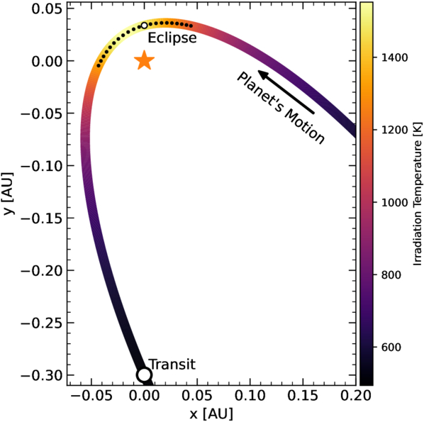
Figure 1. Black circles indicate the span of the NIRSpec observations plotted with 1 hr intervals. The color of the orbit indicates the irradiation temperature, calculated based on the instantaneous star–planet separation and assuming zero albedo and full heat redistribution.
Download figure:
Standard image High-resolution imageSince HD 80606 b was discovered, various models have been generated to study how its atmosphere behaves. Due to its relatively long orbital period, the vertical and horizontal temperature contrasts throughout the planet’s atmosphere are expected to be low during most of the orbit (J. Langton & G. Laughlin 2008; N. Iro & L. D. Deming 2010). During the periapse passage, however, the dayside is rapidly heated, inducing strong acoustic waves (J. Langton & G. Laughlin 2008) and accelerating winds (N. K. Lewis et al. 2017). Depending on the radiative and advective timescales, the rapid heating may imprint a hotspot that periodically appears and disappears as the non–tidally locked planet rotates, causing a “ringing” to be observed in the thermal phase curve (N. B. Cowan & E. Agol 2011; T. Kataria et al. 2013). It has been interpreted that the periastron passage also forms a transient dayside inversion characterized by a rise of ∼400 K with decreasing pressure (N. Iro & L. D. Deming 2010; L. C. Mayorga et al. 2021; S.-M. Tsai et al. 2023b).
As the upper atmosphere gets heated while the planet orbits closer to the star, changes in the abundances and distributions of gases and aerosols are also expected to occur. Assuming chemical equilibrium, methane (CH4), which is predicted to dominate the atmosphere when the planet is less irradiated and cooler, may be converted into carbon monoxide (CO) near periastron (C. Visscher 2012; S.-M. Tsai et al. 2023b). This process is complex and depends on the chemical timescale, efficiency of vertical mixing, and on the abundances of other species that are involved in the CO–CH4 conversion. In addition, photochemical reactions (J. I. Moses et al. 2011; S.-M. Tsai et al. 2021) may deviate the atmospheric properties from chemical equilibrium. By coupling a 3D general circulation model (GCM) with a 1D photochemical model, S.-M. Tsai et al. (2023b) find that, as HD 80606 b’s CH4 is converted into CO, the abundance of water (H2O) also decreases while the abundances of certain photochemical products like hydrogen cyanide (HCN) and acetelyne (C2H2) increase well above what is expected under chemical equilibrium. Comparing condensation curves for various cloud species (C. V. Morley et al. 2012) with HD 80606 b’s temperature changes suggests that clouds may be present throughout much of the orbit. This was explored by N. K. Lewis et al. (2017) using 3D GCMs, which demonstrate that clouds composed of MgSiO3, MnS, and/or Na2S likely persist even during periapse passage; these clouds may effectively raise the photosphere to lower pressures relative to that of a cloud-free atmosphere, thereby changing the observed IR phase curve (J. de Wit et al. 2016; N. K. Lewis et al. 2017).
All of the theoretical predictions developed for eccentric hot Jupiters in general and for HD 80606 b in particular depend on certain assumptions about the planet’s rotation period, internal heating, and atmospheric composition. The first empirical insights into HD 80606 b’s atmospheric dynamics and thermal properties were derived using the 30 hr 8.0 μm and 80 hr 4.5 μm partial phase curves obtained with Spitzer during the planet’s periapse passage. G. Laughlin et al. (2009) and J. de Wit et al. (2016) derived a radiative timescale of τrad ∼ 4.5 hr near the IR photosphere at atmospheric pressures ∼10–100 mbar. No ringing effect is detected in the 80 hr 4.5 μm planetary light curve (J. de Wit et al. 2016). This is consistent with the estimated rotation period of  derived by J. de Wit et al. (2016) using an energy-conserving semi-analytic atmospheric model (here, Prot corresponds to the atmosphere’s bulk rotation rate including winds and any underlying solid-body rotation). HD 80606 b’s estimated τrad and Prot values are somewhat surprising considering theoretical predictions in which (i) cloud-free GCMs computed for HD 80606 b have τrad ∼ 8–12 hr (N. K. Lewis et al. 2017), and (ii) Prot is expected to be ∼40 hr under the assumption that the planet rotates at the pseudo-synchronous rotation period (P. Hut 1981).
While previous IR photometry of HD 80606 b has provided important constraints on our understanding of the seasonal changes occurring in eccentric hot Jupiter atmospheres, wider wavelength coverage at higher spectroscopic resolutions is necessary in order to constrain predictions related to their chemical and thermal properties. The high mass of the planet makes HD 80606 b a relatively poor target for atmospheric characterization via spectroscopy of the planet during transit. While there is potential evidence for an exosphere based on narrowband transit spectroscopy (K. D. Colón et al. 2012), eclipse observations in particular are necessary to learn more about the characteristics of HD 80606 b’s atmosphere.
Here we present near-IR spectroscopic measurements of HD 80606 b’s periapse passage—including the eclipse—obtained with JWST’s NIRSpec instrument. In Section 2, we describe the observations and the data-reduction methods. In Section 3, we present our analysis of both the integrated white-light light curves and the spectroscopic light curves. The results of our analysis are presented in Section 4, followed by a discussion and conclusions presented in Sections 5 and 6.
2. Observations
HD 80606 was observed using JWST’s NIRSpec instrument in BOTS mode with the G395H/F290LP grating/filter combination as part of the GO-2488 program (PI: Sikora). A total of 13,818 exposures were obtained over a 20.9 hr observing window from 2022 November 1 at 06:25 UTC to 2022 November 2 at 03:11 UTC. The observations were briefly interrupted during two  intervals for High Gain Antenna (HGA) moves: once during the eclipse (BJD = 2459885.164) and once approximately 1 hr after periastron (BJD = 2459885.320). The SUB2048 subarray was read out using the NRSRAPID read-out pattern, and we used five groups for each exposure (corresponding to a
  exposure time) in order to avoid saturation for this bright target (J = 7.702 mag).
Since the data presented in this work correspond to a partial rather than a full phase curve, we do not have a clear baseline that can be used to robustly remove certain systematic trends that are impacting the data. Therefore, carrying out independent reductions is necessary to assess how the systematics may be impacted by the reduction process. We carried out two entirely independent data reductions starting from the uncalibrated FITS files: one using the Eureka! pipeline (T. Bell et al. 2022) and a second using a custom pipeline. We find that both reductions yield comparable results both in terms of the trends seen in the extracted planetary phase-curve properties and in the systematic trends seen in the NRS1 and NRS2 measurements (presented in Section 4.2). We adopted the Eureka!-based reduction as the nominal one due to the lower scatter in the light curves and in the derived phase-curve parameters associated with the spectral light curves.
2.1. Eureka! Reduction
The Eureka! pipeline (T. Bell et al. 2022) combines the first two stages of STScI’s JWST Calibration Pipeline (jwst; H. Bushouse et al. 2024) with a customized optimal spectral extraction routine. We used version 1.1 of the Eureka! Python package and 1.15.1 of the jwst Python package. Calibration reference files were taken from context 1303 of version 1.16.1 of the Calibration Reference Data System (CRDS). As briefly described below, we largely adopted the Eureka! settings for stages 1–3 that are recommended for NIRSpec/G395H BOTS-mode observations while also making adjustments that were found to decrease the scatter in the white-light light curves. The settings that were used are defined in the .ecf control files, which we include in the data.tar.gz archive in the online version of this paper for reference.
In Stage 1 of the pipeline, the measured ramps are fit to get the count rates for each exposure. Bad pixels identified using the “mask” reference FITS file from the CRDS were masked (0.5% of NRS1 pixels and 2.8% of NRS2 pixels). Saturated pixels were flagged using the thresholds defined in the NRS1 and NRS2 “saturation” reference FITS files; these flags were then expanded using the Eureka! update_sat_flags keyword with dq_sat_percentile set to 50 and the expand_prev_group option enabled. An average of 9 pixels per integration (0.01%) were found to be saturated for NRS1 and 162 pixels per integration (0.2%) were saturated for NRS2. Group-level column-by-column background subtraction was carried out by fitting a zeroth-order polynomial to the counts in those pixels that are at least 8 pixels away from the trace (masktrace set to True and expand_mask set to 8), where a 6σ threshold was adopted to remove outliers. We skipped the photometric calibration step in Stage 2 because it allows for a straightforward calculation of the photon noise limit using the electron counts.
In Stage 3, Eureka! performs an optimal spectral extraction routine. For NRS1, the spectra were extracted across columns 610 through 2044, while for NRS2, we used columns 5 through 2040. Outliers rejection along the time axis was carried out for each pixel using a 6σ rejection threshold. A Gaussian fit was used to identify the position of the source along each column (src_pos_type=Gaussian). We found that supersampling each centroid by a factor of 3 using the super_sample parameter helped to reduce the scatter in the measured centroid positions and in the extracted white-light light curve. Background subtraction was carried out by removing the median flux calculated from pixels ≥8 pixels away from the source position while removing >6σ outliers (p3thresh=6). The spectral extraction used an aperture with a half-width of 4 pixels. We also tried using a half-width of 2 pixels but this led to a significantly higher white-light curve scatter. Outliers rejection was carried out as part of steps 5 and 7 of the optimal spectral extraction routine using p5thresh=6 and p7thresh=6. Thirteen integrations potentially affected by the two HGA moves noted in Section 2 were manually removed across all wavelength channels along with one NRS1 light curve that was removed due to anomalous flux values, which can be seen in Figure 2 as the column near 3.1 μm showing lower/higher pre-/post-eclipse flux relative to adjacent columns. Sigma clipping was then carried out for each detector’s 1434/2035 wavelength channels with 6σ outliers being removed (1239 measurements in total for NRS1 and 2080 measurements for NRS2, or <0.01%).
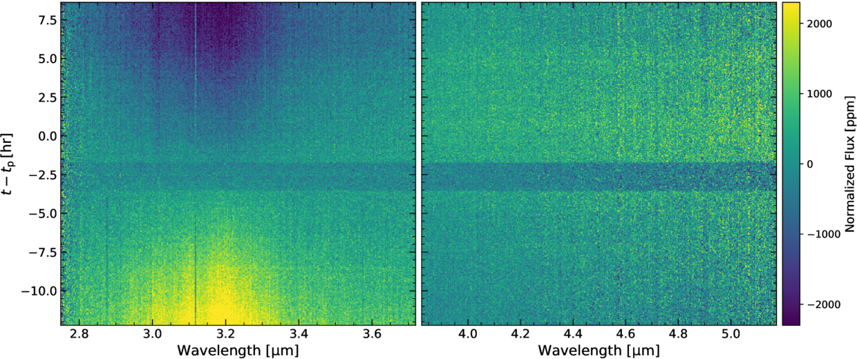
Figure 2. Observed NRS1 (left) and NRS2 (right) flux obtained using the Eureka! reduction pipeline and normalized by the median spectrum. Masked pixels were linearly interpolated over time and then over wavelength for easier visualization. The eclipse is visible near t − tp = −2.6 hr in both detectors. The increase in the planet flux—peaking shortly after periapse—is also easily identifiable in the NRS2 detector. For the NRS1 spectra, systematic wavelength-dependent trends are apparent with the largest impact occurring near 3.2 μm.
Download figure:
Standard image High-resolution imageWhite-light light curves and spectral light curves were generated by binning the flux values extracted from Stage 3 across each wavelength channel bin, where the spectral wavelength bins are defined using a 0.1 μm bin width (R ∼ 40), resulting in 10 bins for NRS1 and 14 bins for NRS2. Finally, we carried out an additional iteration of sigma clipping for each of the wavelength-binned light curves. This did not remove any flux measurements from the NRS1 white/spectral light curves, while two points for the NRS2 white-light curve were removed and 8–17 points were removed from each of the NRS2 spectral light curves.
The NRS1 and NRS2 white-light light curves have an rms scatter of 163 ppm and 217 ppm, respectively. In Figure 2, we show the flux obtained from the Eureka! pipeline normalized by the median spectrum. The eclipse (occurring ≈2.6 hr before periapse) is visible in both the NRS1 and NRS2 detectors. The rise in the planet’s flux following the eclipse is also clearly visible in the NRS2 detector but is somewhat obscured in NRS1 due to significant wavelength-dependent systematic trends, particularly at wavelengths <3.5 μm.
2.2. Custom Pipeline
A fully custom, independent pipeline was written to validate the analysis from Section 2.1. The pipeline corrects for instrumental effects and extracts the spectrophotometry using difference-imaging techniques. Nonlinearity and superbias corrections are made using identical reference pixels as described in Section 2.1. Reference pixels corrections used simple means with 3σ rejection for outliers. The pipeline starts with Stage 0 data products (e.g., “uncal.fits”) and uses the saturation map reference files for NRS1 and NRS2 to flag any group during an exposure that exceeds saturation. Saturated group values for each pixel were excluded when integrating “up-the-ramp” to estimate the electron counts for each pixel for each integration. Superbias, reference pixel, and nonlinearity corrections are then applied. Bad pixels were flagged through saturation or nonzero values of bit 0 from the data-quality flags. Bad pixels were replaced by the mean of a 3 × 3 box centered on the offending group value.
The pipeline uses a two-step process to calculate count rates and to correct for 1/f noise using difference images. The first step uses linear regression to estimate residual bias (zpt) and the integrated electron count rate. Column and row means of the zpt values for each integration were computed and then used as an additional bias correction for each group image. A stacked median image for each group step was calculated using all valid integrations. This provides five 32 × 2048 deep stacks based on 13,818 integrations. Difference images for each group set are then used to correct for 1/f noise using column medians. Only pixels more than 9 pixels away from the spectral trace were used when calculating the median. The 1/f-corrected groups were used to then calculate count rates based on a robust mean of forward differences, with outliers excluded at the 2σ level.
A median image was then used to calculate difference time-series images. Aperture photometry along the spectral trace using an aperture radius of 4 pixels was used to extract the difference spectrum using both difference and nondifference images. The median of the spectrophotometry from nondifference images was used to estimate the photometric zero-point to calculate the scaling necessary to convert differential counts to relative spectrophotometry.
We estimate 200 ppm and 268 ppm rms scatter for the NRS1 and NRS2 white-light light curves obtained from this custom reduction pipeline, respectively. These correspond to 1.2× the rms scatter obtained from the Eureka! reduction.
3. Analysis
3.1. Analytic Light-curve Model
We fitted the light curves obtained from the NRS1 and NRS2 detectors using an analytic model consisting of five components: (i) a planet flux (Fp), (ii) a constant stellar flux (F0), (iii) an additive sinusoidal term to remove flux variations caused either by the star or by instrumental systematics ( ), (iv) a multiplicative polynomial term (Fpoly), and (v) a multiplicative systematics term (Fsys) such that

For the planet flux, we adopted the asymmetric Lorentzian model proposed by N. K. Lewis et al. (2013) in their analysis of Spitzer phase-curve measurements of the eccentric hot Jupiter HAT-P-2 b. The model has four parameters corresponding to the phase-curve amplitude (c1), which we define in terms of F0, the peak offset time (c2), and the timescales over which the flux rises (c3) and decays (c4) with respect to the phase-curve peak:


The symmetric version of this model corresponds to the case in which c3 = c4. The eclipse was modeled using the batman Python package (L. Kreidberg 2015) and depends on the orbital period (Porb), eccentricity (e), inclination angle (i), argument of periastron (ω), eclipse midpoint (Te), the ratio of the semimajor axis to the stellar radius (a/R⋆), and the ratio of the planetary radius to R⋆ (Rp/R⋆). Since the partial phase-curve observations we obtained span only a small fraction of the 111.4 days orbit and do not include the transit, we opted to fix Porb, e, i, ω, a/R⋆, and Rp/R⋆ at published values (see Table 1), which have been precisely measured using transit, eclipse, and RV measurements (K. A. Pearson et al. 2022). The eclipse midpoint, however, was allowed to vary as a free parameter when fitting the integrated white-light light curves.
Table 1. Published Stellar and Planetary Properties Associated with HD 80606 b that Were Used in This Study
| Parameter | Value |
|---|---|
| Teff (K) | 5565 ± 92a |
| R⋆ (R⊙) | 1.066 ± 0.024a |
| M⋆ (M⊙) | 1.047 ± 0.047a |

| 4.402 ± 0.039b |
| [Fe/H]⋆ | 0.348 ± 0.057a |
| Mp (MJup) | 4.1641 ± 0.0047c |
| Rp (RJup) | 1.032 ± 0.015c |

| 0.01019 ± 0.00023c |
| Porb (day) | 111.436765 ± 0.000074c |
| a (au) | 0.4603 ± 0.0021c |
| e | 0.93183 ± 0.00014c |
| ω (deg) | −58.887 ± 0.043c |

| 58888.07466 ± 0.00204c |
Notes.
aL. J. Rosenthal et al. (2021). bCalculated from the published M⋆ and R⋆. cK. A. Pearson et al. (2022).Download table as: ASCIITypeset image
The NRS1 measurements are dominated by a systematic downward slope in flux between the start and end of the observing window that is strongly wavelength dependent (Figure 2). Similar slopes have previously been reported for NIRSpec time-series observations (e.g., L. Alderson et al. 2023; S. E. Moran et al. 2023). We account for these variations by including a multiplicative polynomial term,

where pn are free parameters and t0 is the approximate eclipse midpoint time, which we fix at BJD = 2459885.165. No such systematic slope is visible by eye in the NRS2 white-light light curve, however we include the Fpoly term in the model selection process described below.
In Figure 3, the panels labeled (a)–(d) show the NRS1 and NRS2 white-light light-curve flux and residuals obtained using the simplest model that produces an adequate overall fit to the data (discussed further in Section 4.1). For NRS1, this model consists of the star and planet contributions (F0 and a symmetric Fp) and a 2nd-order Fpoly term, while NRS2-only includes F0 and Fp. The residuals show correlated noise that we attempt to capture with the Fsys and  terms. The sinusoidal term is defined as

where A1 and B1 are free parameters included so as to allow the total amplitude to vary linearly over time, and tini is the timestamp of the first exposure. The phase ϕ1 is included as a free parameter, and the frequency f1 is fixed at the highest-amplitude frequencies identified in Lomb–Scargle periodograms (N. R. Lomb 1976; J. D. Scargle 1982) calculated from the residuals shown in Figure 3. These periodograms exhibit maximum-amplitude peaks at frequencies of 0.174 hr−1 (5.7 hr) and 0.231 hr−1 (4.3 hr) for the NRS1 and NRS2 light curves, respectively.
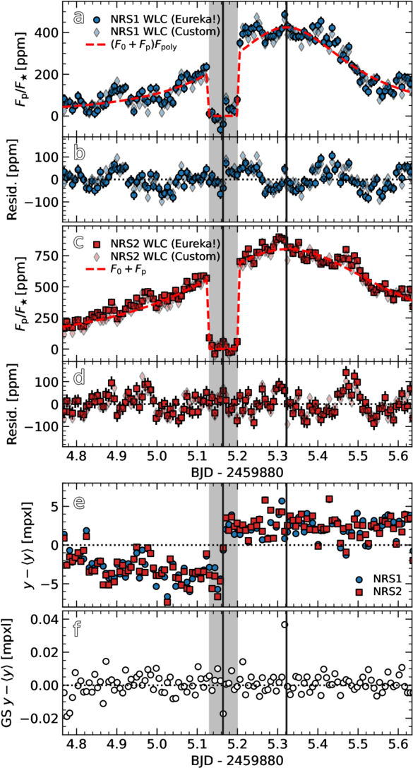
Figure 3. Binned NRS1 and NRS2 white-light light curves and their residuals (panels (a)–(d)) obtained using a model that includes only the planet phase curve and, in the case of NRS1, a 2nd-order polynomial term (red dashed line). The darker circles/squares are from the Eureka! reduction and the fainter diamonds are from the independent custom reduction, which have comparable error bars but are not shown for visual clarity. Panels (e) and (f) show the relative centroid positions obtained from the Eureka! NRS1 and NRS2 reductions and the centroid positions associated with the guide star. All points have been binned using  bin widths. The shaded region highlights the in-eclipse measurements, and the vertical black lines indicate the two HGA moves.
Download figure:
Standard image High-resolution imageThe bottom two panels (e) and (f) of Figure 3 show the NRS1 and NRS2 centroid positions in the dispersion direction (y) obtained from the Eureka! reduction as well as the guide-star centroid y-position (yGS). We find that both y(t) and yGS(t) show variability, most notably during the first HGA move that occurs near the middle of the eclipse. The NRS1 residuals show a jump in flux for both the Eureka! reduction and for the custom reduction that also coincides with the first HGA move, while no similar jump is apparent in the NRS2 residuals. This suggests that the measured NRS1 flux may be correlated with the centroid position due to intrapixel variations as found in Spitzer and Hubble Space Telescope (HST) time-series observations (e.g., J.-M. Désert et al. 2009; D. K. Sing et al. 2019). To account for this jump in flux and any other correlations with y and yGS, we include an Fsys term defined as

where cy and cGS,y are free parameters, and  corresponds to y(t) after removing the jump, which is done by splitting the time series at the first HGA move and dividing the two segments by their median values. Both
  and yGS(t) are normalized by subtracting the mean and dividing by the standard deviation. The jump in flux is corrected using a step function, ΔFjump(t), given by

where ΔFjump and Tjump are free parameters. In Section 4, we discuss how the nominal models for the NRS1 and NRS2 light curves were ultimately selected.
The best-fitting parameters and uncertainties for the analytic light-curve modeling were derived using the emcee ensemble sampler Python package (D. Foreman-Mackey et al. 2013, 2019). For each light curve, 24–48 walkers were initialized, generating chains ≳5 × 10⁴ steps in length after discarding the first 5000 steps as burn-in. Sampling was continued until the number of steps exceeded 50 times the mean autocorrelation lengths. The  statistic (A. Gelman & D. B. Rubin 1992) was then used to check for convergence where additional samples were generated until
  for each parameter. For both the white-light light-curve fits and the spectral light-curve fits, we used uniform priors for all parameters. In all cases, we also included a “jitter” term (σJit, sampled in log space) that is added to the formal measurement uncertainties in quadrature, which accounts for additional white noise that may be present in the data. This increase in the measurement errors ultimately imposes a reduced χ2 of ≈1.
3.2. Atmospheric Retrievals
We carried out two sets of atmospheric retrievals using two independent frameworks. Within one framework, we used forward models calculated with petitRADTRANS (P. Mollière et al. 2019) in which the atmosphere is assumed to be in chemical equilibrium. The chemical composition of the atmosphere is determined by the bulk metallicity ([M/H]) and C/O ratio. The abundances are interpolated from a grid computed using easyCHEM (for more details, see P. Mollière et al. 2017) and do not incorporate photochemical reactions. We included opacities from gas-phase H2O, CO, CO2, and CH4, which are expected to be the predominant contributors to the total atomic and molecular opacity within the NRS1/NRS2 bandpasses. Continuum opacities associated with H2–H2 and H2–He collision-induced absorption and H2 and He Rayleigh scattering were also included. Clouds composed of MnS and/or MgSiO3 could potentially be present during the observed phases (N. K. Lewis et al. 2017). In order to account for these species, we include a gray cloud deck in which the flux emitted by layers below the cloud deck pressure (Pcloud) is blocked at all wavelengths. The model atmosphere was defined using 100 layers logarithmically distributed from 100 bar to 1 μbar, with a temperature defined using the four-parameter profile proposed by T. Guillot (2010), described by the IR absorption coefficient (κIR), the ratio of optical to IR absorption coefficients (γ), the planet’s interior temperature (Tint), and the irradiation temperature (Tirr). Posterior distributions were derived using emcee in which 16 walkers were initialized and 105 samples per walker were generated, with the first 104 steps being discarded as burn-in. After removing chains stuck in low-probability regions (between zero and five chains), we obtained ∼106 samples. Uniform priors were adopted for all parameters.
The second retrieval framework used forward models calculated with PyratBay (P. E. Cubillos & J. Blecic 2021) in which we include all of the opacity sources used in the petitRADTRANS-based retrievals listed above. In this case, the abundances are uniform with pressure and are allowed to vary freely. We used the same pressure–temperature (PT) profile, cloud deck, and adopted a model atmosphere of 61 layers with a minimum pressure at the top of the atmosphere of 100 μbar. We sample the parameter space with MC3 using the snooker differential-evolution Markov Chain Monte Carlo algorithm (P. Cubillos et al. 2017). We initialize with 32 parallel chains for a total of 4 × 10⁶ samples, with the first 105 steps discarded as burn-in. We similarly adopt uniform priors for all parameters.
4. Results
4.1. White-light Light Curves
Each of the integrated NRS1 and NRS2 white-light light curves obtained from the Eureka! reduction were fitted using the modeling framework described in Section 3.1. Bayesian information criterion (BIC) values were calculated for several variations of the general light-curve model in order to select the most statistically significant model with the fewest parameters. Specifically, the goal is to determine whether Fpoly should be included in the model and what polynomial order is preferred by the data, whether a symmetric or asymmetric planet phase curve is preferred, and whether the  components should be included. The model selection process involves three steps: (i) we fit the data without including an
  term and using a symmetric/asymmetric Fp model and an Fpoly term up to 3rd order; (ii) we then test whether including the ΔFjump(t) term significantly decreases the BIC (where ∣ΔBIC∣ > 5 is considered significant); and (iii) whether including the
  term significantly decreases the BIC.
4.1.1. NRS1 White-light Light Curve
Based on step (i) of the model selection process, we found that the NRS1 white-light light curve favors a symmetric phase-curve model with a 2nd-order polynomial term, which has a ∣ΔBIC∣ > 10 compared to the models using a 1st- or 3rd-order Fpoly term and symmetric/asymmetric Fp model. For steps (ii) and (iii) of the model selection, we found that including both a ΔFjump(t) term and an  term produced a large decrease in the BIC values: Relative to the symmetric Fp, 2nd-order Fpoly model, including ΔFjump(t) decreases the BIC by 86, and including
  decreases this by an additional 244. Therefore, the nominal model we adopted for the NRS1 white-light light curve consists of a 2nd-order Fpoly, symmetric Fp, and nonzero ΔFjump and
  terms, and includes 15 free parameters (F0, c1, c2, c3, Te, p1, p2, cy, cGS,y, A1, B1, ϕ1, ΔFjump, Tjump, and σJit).
The fit to the Eureka!-reduced NRS1 white-light light curve using the nominal model is shown in Figure 4 and the derived parameters are listed in Table 2. We find that the model achieves a precision of 2.01× the 81 ppm photon noise limit. We also fit the light curve obtained from the custom reduction pipeline (see Section 2.2), for which we obtain a lower precision of 2.44× the photon noise limit. Some red noise is still present in the residuals as seen by eye in Figure 4 and indicated in the Allen deviation plot shown in Figure 13 of the Appendix. The measured flux is slightly correlated with y(t) and yGS,y(t) based on the derived cy = − 2.6 ± 1.4 ppm and cGS,y = 2.5 ± 1.4 ppm. The 1st- and 2nd-order polynomial coefficients are significantly nonzero with  and p2 = 3.396 ± 0.078 ppm hr−2. As discussed further in Section 4.2 in the context of the spectral light curves as well as in the Appendix, we derive similarly high magnitudes for p1 and p2 from an analysis of the publicly available NIRSpec/G395H transit observations of GJ486 b (S. E. Moran et al. 2023). This suggests that these polynomial trends are not unique to the HD 80606 NIRSpec data and the analysis presented here.
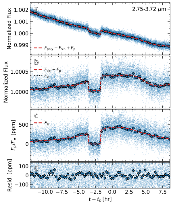
Figure 4. NRS1 white-light light curves, where the dark blue circles are the binned measurements generated using  bin widths and the light blue circles are the unbinned measurements. The x-axis corresponds to time relative to periapse. Panel (a) shows the observed flux obtained using Eureka!. The red dashed line is the best-fitting nominal model (Section 4.1) consisting of a symmetric planet phase curve, a sinusoidal term (
 ) with a frequency of f1 = 0.174 hr−1, and a 2nd-order polynomial term (Fpoly). In panel (b) the observations have been detrended by removing Fpoly, in panel (c) both Fpoly and
  have been removed leaving the planetary signal (Fp), and the residuals are shown in panel (d).
Download figure:
Standard image High-resolution imageTable 2. Parameters Derived for the NRS1 and NRS2 White-light Light Curves Using the Nominal Models
| Parameter | Nominal NRS1 | Nominal NRS1 | NRS2 |
|---|---|---|---|
| (No Jump) | |||
| F0 (e−/s) | 111550.08 ± 0.80 | 111554.08 ± 0.60 | 36531.35 ± 0.23 |
| c1 (ppm) | 433.6 ± 7.8 | 466.3 ± 8.0 | 812.9 ± 6.9 |
| c2 − tp (hr) |

|

|

|
| c3 (hr) | 5.42 ± 0.18 | 4.62 ± 0.11 | 7.65 ± 0.10 |
| Te (BJD − 2459885) | 0.16528 ± 0.00025 | 0.16487 ± 0.00027 | 0.16421 ± 0.00016 |
| A1 (ppm) |

|

|

|
| B1 (ppm hr−1) | 2.50 ± 0.36 |

| 2.87 ± 0.29 |
| ϕ1 | 0.083 ± 0.011 | 0.0427 ± 0.0091 | 0.831 ± 0.012 |
| f1 (hr−1)a | 0.174 | 0.174 | 0.231 |
| p1 (ppm hr−1) | −153.74 ± 0.76 |

| ⋯ |
| p2 (ppm hr−2) |

|

| ⋯ |
| cy (ppm) | −2.6 ± 1.4 | −2.3 ± 1.7 | −0.6 ± 1.9 |
| cGS,y (ppm) | 2.6 ± 1.4 | 3.0 ± 1.6 | 11.5 ± 1.9 |
| Tjump (BJD − 2459885) |

| ⋯ | ⋯ |

| 77 ± 10 | ⋯ | ⋯ |

|

|

|

|
Notes. For NRS1, we also list the parameters obtained when the ΔFjump parameter is not included in the model. For each parameter, we report the median value calculated from the marginalized posteriors while the uncertainties correspond to 16th and 84th percentiles (1σ).
aFixed at values inferred from residuals calculated for the simplest considered light-curve model (see Figure 3).Download table as: ASCIITypeset image
For the ΔFjump(t) term, we obtain a jump occurrence time of  , which is consistent with the first HGA move, and an amplitude of
  . We note that the jump correction amplitude is correlated with c3 and p1. As a result, the difference in the inferred planet flux when including the jump term is ≈77 ppm near the eclipse midpoint, but is much less further away from this point since the jump in flux is partially absorbed by c3 and p2. Nonetheless, we find that including ΔFjump(t) does have a nonnegligible impact (∼4σ) on the derived c1 and c3 values.
4.1.2. NRS2 White-light Light Curve
For NRS2, step (i) of the model selection process yielded the lowest BIC for the model that includes a symmetric Fp and does not include a polynomial term: For both the symmetric and asymmetric Fp models, including a polynomial increased the BIC by >7. For step (ii), we find that including the ΔFjump(t) term led to a higher BIC and, unlike for the NRS1 white-light light curve, a Tjump that was poorly constrained. However, the BIC does decrease significantly by 148 when including an  term for step (iii). We therefore adopt a nominal model that includes a symmetric Fp, an
  term, and an Fsys term with ΔFjump = 0, which consists of 11 free parameters (F0, c1, c2, c3, Te, cy, cGS,y, A1, B1, ϕ1, and σJit).
The fit to the NRS2 white-light light curve using the nominal model is shown in Figure 5. The derived parameters are listed in Table 2, where we also include for comparison the parameters derived when the jump parameter is not included in the model. The nominal model yields a precision of 2.02× the 108 ppm photon noise limit for the Eureka! reduction and 2.45× the photon noise for the light curve obtained from the custom reduction. As seen in the Allen deviation plot in the Appendix (Figure 13), the NRS2 residuals have red noise with a timescale comparable to that found in the NRS1 residuals.
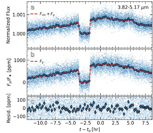
Figure 5. Same as Figure 5 but for the NRS2 white-light light-curve fit with the nominal model, which consists of a symmetric phase curve, a sinusoidal term ( ) with a frequency of f1 = 0.231 hr−1, and no polynomial term. Panel (a) is the observed flux, in panel (b)
  has been removed, and panel (c) shows the residuals.
Download figure:
Standard image High-resolution imageComparing the NRS2 and NRS1 phase curves, we find large differences with the former having a much higher amplitude (c1), peak offset (c2), and rise/decay timescale (c3), which all differ by ≳5σ. The eclipse midpoint times differ by about 4.3σ (BJD = 2459885.16528 ± 0.00025 and BJD = 2459885.16420 ± 0.00016 for NRS1 and NRS2, respectively). This difference may be significant, however when the jump parameter is not included in the NRS1 model, we derive a lower Te that has a ∼2.4σ difference with respect to NRS2. K. A. Pearson et al. (2022) derive an eclipse midpoint of  . Using the reported Porb = 111.436765 ± 0.000074 days, we find a discrepancy between the predicted eclipse time and the value derived from the NRS2 white-light light curve of
  . This discrepancy may be partly attributed to an underestimated uncertainty in the published
  , which K. A. Pearson et al. (2022) note was derived using a fixed ω value (ω = − 58.887 ± 0.043 deg).
The NRS2 bandpass is comparable to the Spitzer 4.5 μm bandpass, allowing for rough comparisons to be made with the phase curve presented by J. de Wit et al. (2016). These authors report an amplitude of 738 ± 52 ppm, and is therefore comparable to our value of 812.9 ± 6.8 ppm. The Spitzer 4.5 μm phase curve has a notably lower peak offset of between ≈ −1 hr and 0 hr relative to periapse (for NRS2, we derive an offset of 1.073 ± 0.040 hr). The timescale over which the planet flux decreases postperiapse is also noticeably higher for NRS2 relative to the Spitzer phase curve: Between the time of peak flux and t − tp ≈ 8 hr (near the end of our observing window), Fp/F⋆ decreases from ≈830 ppm to 450 ppm compared to a decrease of ≈740–180 ppm for Spitzer. On the other hand, the rise in flux from t − tp ≈ –12 hr associated with the two phase curves is in close agreement.
4.2. Spectral Light Curves
Each of the Eureka! spectral light curves (10 for NRS1 and 14 for NRS2) was fitted using the nominal models adopted for the white-light light curves (Section 4.1). For comparison, we also fit the spectral light curves obtained from the custom data-reduction pipeline (Section 2.2). The derived phase-curve parameters associated with each of the NRS1 and NRS2 spectral light curves (and those derived for the white-light light curves) are plotted in Figure 6 along with the polynomial coefficients included in the nominal NRS1 model. In general, we find that the two reductions yield comparable results, which exhibit the same trends but have some systematic discrepancies. Compared to the custom reduction, the Eureka! NRS1 reduction shows ∼2σ higher c1 and p2 values and ∼2σ lower c2 and p1 values, particularly near 3.2 μm. These differences are partly explained by the positive/negative correlation between c1/c2 and p2 and the relatively weak negative correlation between c2 and p1 (see the corner plot in Figure 14 in the Appendix). The NRS2 light curves generally show closer agreement, with typical discrepancies ≲1σ.
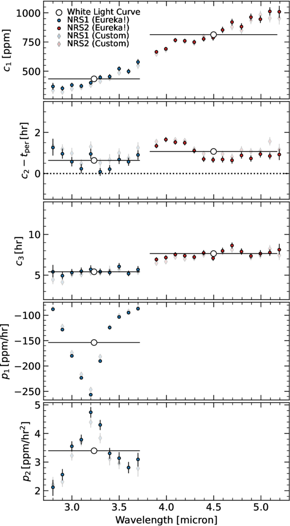
Figure 6. Phase-curve amplitude (c1), peak offset (c2), and rise/decay timescale (c3) along with the polynomial coefficients (p1 and p2). Darker blue and red circles correspond to the NRS1 and NRS2 spectral light curves reduced using Eureka!. White circles are the NRS1/NRS2 white-light light-curve values, where the horizontal error bars indicate the wavelength bin widths. Lighter diamonds are obtained using the custom reduction pipeline. Note that the nominal NRS2 model does not include a polynomial term, which is why there are no associated p1 and p2 terms plotted in the fourth and fifth panels.
Download figure:
Standard image High-resolution imageAs expected based on the observed light curves shown in Figure 2, the linear slope (p1 in Equation (4)) included in the NRS1 model’s polynomial term is highly correlated with wavelength. The distribution of p1(λ) is roughly Gaussian in shape with a maximum magnitude occurring at ≈3.2 μm. The 2nd-order polynomial coefficient (p2) shows a characteristically similar wavelength dependence with a peak occurring at the same wavelength. The highly wavelength-dependent systematics affecting our NRS1 observations are also shown to impact NIRSpec/G395H transit observations of GJ486 b (S. E. Moran et al. 2023; see their Figure 1). Both data sets were obtained using a similar instrument configuration using low group numbers in order to avoid saturation (HD 80606 was observed using five groups while those of GJ486 used three). We analyzed the out-of-transit baseline exposures from the publicly available GJ486 data in order to characterize the wavelength dependence of p1 and p2 (see the Appendix). This analysis yields a similar Gaussian-like trend in p1(λ), while p2 is nearly constant for λ ≳ 3.1 μm with a value of ≈60 ppm hr−2 (Figure 15).
The phase-curve amplitudes (c1) show a nearly monotonic increase with wavelength from ∼400 ppm at 2.8 μm to ∼1000 ppm at 5.2 μm. Small decreases in c1 are apparent at ≈3.0–3.5 μm and at ≈4.2–5.1 μm. Similar decreases are apparent in the peak offset (c2), which range from ≈0 to 1.3 hr within the NRS1 bandpass and from ≈0.5 to 1.5 hr within NRS2. A sharp increase in c2 coinciding with the minimum p1 value and the maximum p2 value near 3.2 μm is apparent. As noted above, the c2 parameter is negatively correlated with p2 and, to a lesser extent, p1; therefore some of the increase in c2 may be due to the decrease in p1. Lastly, the rise/decay timescale (c3) shows a gradual increase across both the NRS1 and NRS2 wavelengths ranging from ≈5 to 9 hr along with small decreases, most notably at 4.5 μm and 4.9–5.2 μm. We note that while the polynomial terms included in the NRS1 model may somewhat bias the inferred phase-curve parameters, the NRS2 light curves, which do not have obvious wavelength-correlated noise, show comparable trends.
4.3. Phase-resolved Planet Spectra
We used the fitted spectral light curves to extract the planet-to-star flux contrast (Fp/F⋆) and the planet’s brightness temperatures (Tbright) at several phases in order to identify and characterize any time variability in the planet’s emission spectrum. Eclipse depths were calculated from the mean Fp/F⋆ values associated with the phase-curve model averaged over a 2 hr window centered on the eclipse midpoint. We then carried this out for nine additional phases totaling four pre-eclipse phases and six post-eclipse phases. The Fp/F⋆ spectra are presented in Section 4.4 alongside the atmospheric retrieval results. For reference, all 10 spectra are shown in Figure 16 in the Appendix, where we include both the nominal spectra obtained from the Eureka! reduction and the spectra obtained from the custom reduction.
Brightness temperatures were calculated for each wavelength and orbital phase using the Fp/F⋆ measurements. The stellar spectrum used to derive the planet’s thermal emission (Fp) was estimated using a PHOENIX model with Teff = 5600 K,  , and [M/H] = 0.5. Instrumental broadening assuming R = 2700 was applied to the model stellar spectrum, which was then interpolated onto the native NIRSpec resolution and binned using the 0.1 μm bin widths adopted for the observed spectral light curves. The planet-to-star radius ratio used for the calculation of Tbright was taken to be
  (K. A. Pearson et al. 2022). The brightness temperatures derived for five of the 10 phases spanning the observing window are shown in Figure 7. Comparing Tbright calculated from both the Eureka! and the custom reduction pipelines shows generally good agreement. During the preperiapse phases, the Eureka! reduction yields Tbright values within the NRS1 bandpass that are systematically higher than the custom reduction by ∼50 K, while the NRS2 wavelengths agree within ≲1σ. The NRS1 discrepancy may be attributed to the correlation between the c1/c2 phase-curve parameters and p2 noted above in Section 4.2.
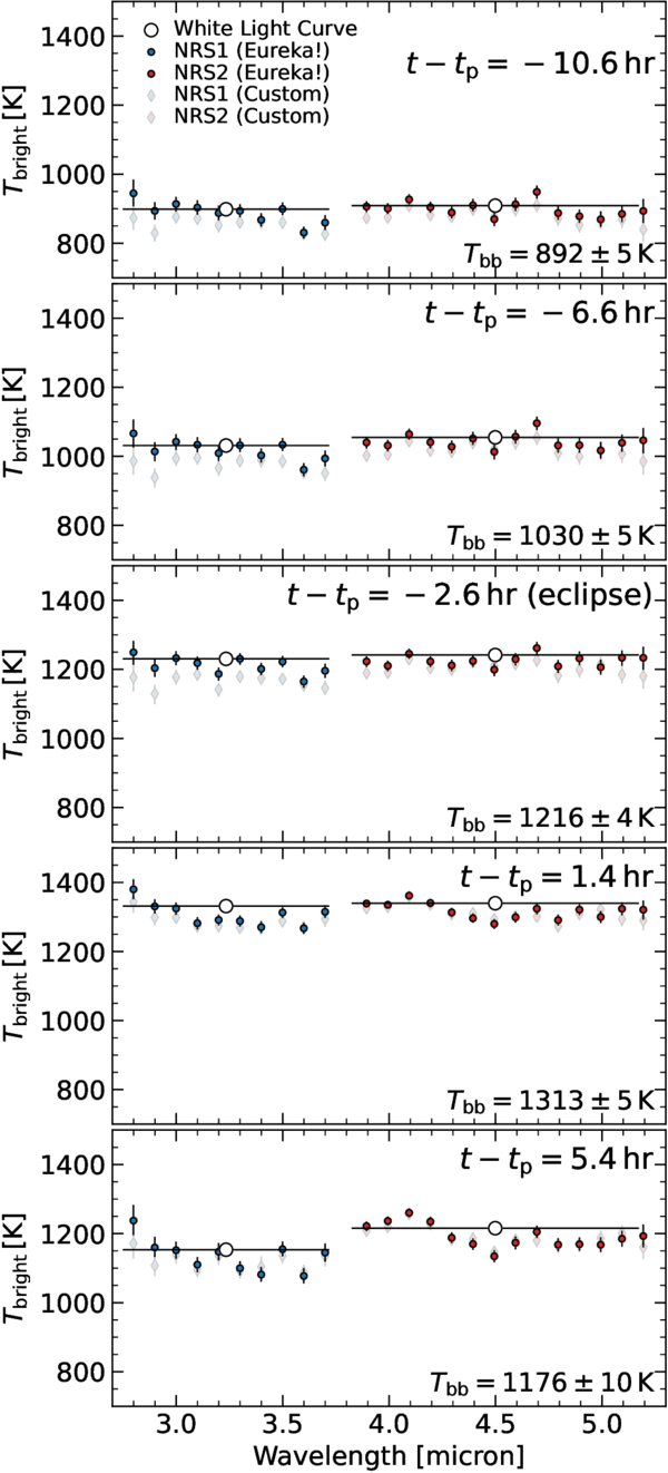
Figure 7. Brightness temperatures derived using the nominal NRS1 and NRS2 light-curve models for the Eureka! reduction (dark circles) and for the custom reduction pipeline (light diamonds). The estimated blackbody temperatures (Tbb) derived by fitting a blackbody spectrum to the NRS1 and NRS2 Fp/F⋆ measurements while including a flux offset for NRS1 (see Section 4.3) are shown for each phase. White circles correspond to values calculated from the white-light light curves.
Download figure:
Standard image High-resolution imageNext, we proceeded to fit the Fp/F⋆ spectra for each phase assuming that the planet radiates as a blackbody. Best-fitting blackbody temperatures and uncertainties were estimated by minimizing the χ2 values using the curve_fit function from the scipy Python package, where the stellar flux is given by the PHOENIX stellar model noted above. Fits were carried out using the Eureka!-reduced light curves for three detector configurations: using both NRS1 and NRS2 measurements; using both NRS1 and NRS2 measurements while also including an additive flux free parameter to the NRS1 measurements (fNRS1) in order to account for possible offsets related to the instrument or introduced by the NRS1 light-curve polynomial detrending term; and using only the NRS2 measurements. In all three cases, we find a similar trend in which the first six phases have relatively low reduced-χ2 values ( ) compared to the last four phases (
 ). Comparing the derived Tbright values for the NRS1+NRS2 and NRS1+NRS2+fNRS1 cases, we find discrepancies of 0.5–2.6σ, with the last three phases showing the largest differences. Slightly larger discrepancies are found when comparing the NRS1+NRS2 and NRS2-only configurations (0.8–2.6σ), while the NRS1+NRS2+fNRS1 and NRS2-only cases show negligible differences (≲0.5σ). The Tbright values for case 1 are shown in Figure 7, which increase from 892 ± 5 K at the start of the observing window to a peak value of 1313 ± 5 K during the first postperiapse phase (t − tp = 1.4 hr) before decreasing to 1077 ± 10 K.
In Figure 7, the postperiapse phases show the largest deviations from a blackbody, with the appearance of several potential absorption features. Within the NRS2 bandpass, a decrease in Tbright is found at λ > 4.3 μm, which is qualitatively consistent with CO and CO2 absorption (see recent NIRCam eclipse measurements of HD 149026 b; J. L. Bean et al. 2023). Within the NRS1 bandpass, a decrease in Tbright is found from 3.1 to 3.4 μm, which may be due to absorption by CH4 (see NIRCam eclipse measurements of WASP-80 b; T. J. Bell et al. 2023). These features are discussed further below.
4.4. Atmospheric Retrievals
We carried out the petitRADTRANS-based chemical-equilibrium atmospheric retrievals described in Section 3.2 for the three instrument configurations that we considered in conjunction with the blackbody model (Section 4.3): the NRS1+NRS2 case, the NRS1+NRS2+fNRS1 case, and the NRS2-only case. BIC values were then calculated for the maximum a posteriori (MAP) solutions obtained from these retrievals and were compared with the blackbody spectrum MAP solution BIC values. We find that for both the NRS1+NRS2 and NRS1+NRS2+fNRS1 cases, the chemical-equilibrium model is preferred over a simple blackbody spectrum for the four postperiapse phases. This is based on the calculated ΔBIC values ranging from −6 to −112, where the NRS1+NRS2 case exhibits the largest differences (<−16); for the NRS2-only case, the chemical-equilibrium model is preferred only for the last three phases (−25 < ΔBIC < −16). For each of the four phases in which we find significant deviations from a blackbody spectrum, we carried out a similar BIC comparison between the petitRADTRANS-based chemical-equilibrium retrievals and the PyratBay-based free retrievals. Both modeling frameworks yield comparable χ2 values and the chemical-equilibrium model, having fewer free parameters, is favored over the free retrievals. Therefore, based on the quality of fits provided by each considered model, we conclude that during the first six phases the observed spectrum is indistinguishable from a blackbody spectrum; the last four phases are best characterized by a chemical-equilibrium model atmosphere, and do not show evidence of disequilibrium chemistry or photochemistry.
In Figure 8, we show the results of the chemical-equilibrium retrievals carried out for the NRS1+NRS2 case at the eclipse phase (t − tp = −2.6 hr) and at the second postperiapse phase (t − tp = 3.4 hr). The left columns compare the observed spectra with models generated from the retrieval posteriors and with the GCM-based predictions published by S.-M. Tsai et al. (2023b). The GCM-based predictions assume a solar-metallicity atmosphere with a 100 K internal temperature. The right column shows the derived PT profile constraints along with the GCM PT profiles. All four of the postperiapse spectra and PT profiles are also shown in Figure 18 of the Appendix. We find that the PT profiles derived from the chemical-equilibrium retrievals for all three detector combinations are consistent in terms of the overall profile shape and in terms of their photospheric temperatures at pressures of 1–10 mbar. Similar agreement is found when comparing the profiles derived from the chemical-equilibrium and PyratBay-based free retrievals for the NRS1+NRS2 case. During the first five phases through the eclipse (−10.6 ≤ t − tp ≤ −2.6 hr), the derived blackbody temperatures and photospheric temperatures associated with the retrievals are notably higher than those of the GCM PT profiles. Phases six and seven (−0.6 ≤ t − tp ≤ 1.4 hr) show good agreement, while the GCM temperatures are higher during the last three phases. These differences are manifest in the spectra as a vertical shift across the observed bandpasses (see Figure 16 in the Appendix). Additionally, none of the retrieved PT profiles show clear evidence of an inversion near the IR photosphere as found in the GCMs, and no obvious emission features are seen in the extracted NIRSpec spectra that would otherwise indicate an inversion.
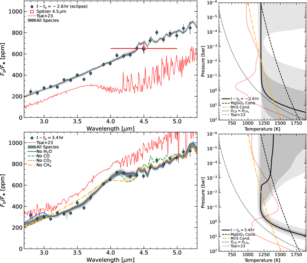
Figure 8. Results obtained from the petitRADTRANS-based chemical-equilibrium retrievals for two phases: at the eclipse (top row), which is consistent with a blackbody with a 1219 ± 23 K temperature, and at the eighth extracted phase (bottom row), which shows the maximum CH4 detection significance. Left column: the observed NRS1 (λ < 3.8 μm) and NRS2 (λ > 3.8 μm) emission spectra (blue circles) compared with the 1σ (dark gray) and 2σ (light gray) uncertainty bands from the retrievals. The MAP chemical-equilibrium solutions obtained when removing one of the four included gaseous opacities, which were calculated to evaluate the detection significance, are plotted for the bottom row. The red square is the 4.5 μm Spitzer eclipse depth (J. de Wit et al. 2016). Right column: PT profiles derived for the retrievals, where the solid black line is the median profile and the dark/light bands indicate 1σ/2σ uncertainties. The faint red lines are the GCM-based profiles published by S.-M. Tsai et al. (2023b) assuming a solar metallicity and Tint = 100 K. The dotted line indicates points at which CO and CH4 are in equal abundance for a solar-metallicity atmosphere in chemical equilibrium (J. J. Fortney et al. 2020), while the yellow dashed–dotted and black dashed lines are the condensation curves for MnS and MgSiO3 (C. Visscher et al. 2010; C. V. Morley et al. 2012).
Download figure:
Standard image High-resolution imageThe posteriors for the pressure of the gray cloud deck included in the retrievals are poorly constrained during the first six phases. For the post-eclipse phases, we obtain 2σ lower limits on the cloud deck’s altitude at pressure layers Pcloud ≳ −0.8 bar for the chemical-equilibrium retrievals and Pcloud ≳ −1.1 bar for the free retrievals (i.e., below the 1–10 mbar IR photosphere). As shown in Figure 8, the increase in temperature occurring from the pre- to postperiapse phases is such that the photospheric temperatures reach the condensation point of MnS clouds (yellow dashed–dotted line; C. V. Morley et al. 2012), suggesting that such clouds, if present, are expected to dissipate during the 21 hr observing window (discussed further in Section 5).
We estimated the detection significance of H2O, CO, CO2, and CH4 for the last four extracted phases using a similar method as presented by T. Bell et al. (2022). This involves carrying out additional chemical-equilibrium retrievals using petitRADTRANS with each of the four gas species being excluded from the model one at a time. We used emcee to generate 16 chains 2 × 10⁴ steps in length each with the first 104 steps discarded as burn-in, yielding 1.6 × 10⁵ samples. From these samples we then selected the maximum-likelihood solution and compared the associated χ2 value with that obtained when including all gas species. The resulting significance levels for each molecule and for each phase are shown in Figure 9. Adopting a 3σ threshold, we find that the NRS1+NRS2 case yields detections of CH4 (6.1–10.7σ), H2O (4.2–5.5σ), and CO (3.7–4.4σ). CH4, CO, and CO2 have >3σ significance levels for the NRS1+NRS2+fNRS1 case (4.1–5.7σ, 3.8σ, and 4.1σ, respectively) while only CO is detected for the NRS2-only case (3.6σ).
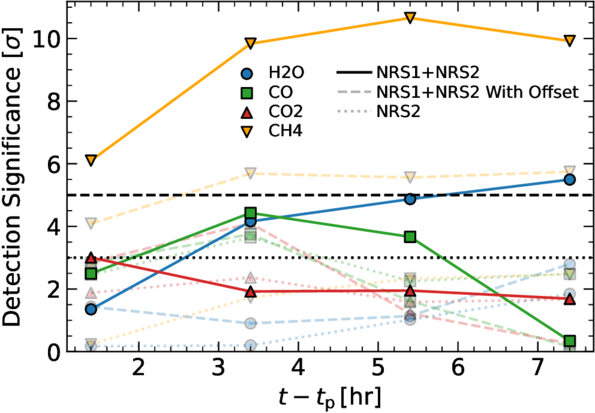
Figure 9. Detection significance levels estimated for each molecule at each of the five postperiapse phases (where the x-axis corresponds to time relative to periapse). Dark symbols/solid lines are obtained using both NRS1 and NRS2, light symbols/dashed lines use NRS1 and NRS2 with a flux offset, and light symbols/dotted lines use only NRS2.
Download figure:
Standard image High-resolution imageThe MAP solutions found for the four models without H2O, CO, CO2, or CH4 are overplotted in Figure 8 and in Figure 18 of the Appendix; comparing these with the solutions obtained using all species demonstrates which wavelength channels have the largest contribution to the estimated detection significance. Both the CO and CO2 absorption bands are primarily found within the NRS2 bandpass and therefore should be detectable when using only NRS2. Since CO2 is not detected in this case and is only detected during a single phase for the NRS1+NRS2+fNRS1 case, the detection is not considered to be reliable.
In Figure 10, the C/O ratio and metallicity ([M/H]) derived from the petitRADTRANS chemical-equilibrium retrievals are plotted for the last four phases using all three instrument configurations. The NRS2-only configuration exhibits solar C/O and [M/H] values for each phase and has the largest uncertainties due to the exclusion of the NRS1 bandpass, but is also not impacted by potential flux offsets. During the last three phases, these C/O and [M/H] values are in agreement with the NRS1+NRS2 case, where the highest precision is obtained for the last phase (C/O = 0.49 ± 0.15 and [M/H] = −0.17 ± 0.31). Supersolar C/O and [M/H] values are obtained for the first postperiapse phase in the NRS1+NRS2 case and for the first to third postperiapse phases when including fNRS1. These instances are all associated with nondetections of H2O, which therefore likely biases the inferred C/O and [M/H], since within the petitRADTRANS chemical-equilibrium model framework C/O is controlled by varying the total O abundance.
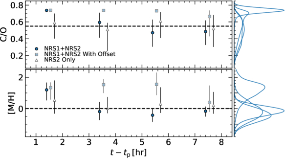
Figure 10. Atmospheric compositions inferred from the chemical-equilibrium retrievals for the four postperiapse phases that deviate from a blackbody spectrum. We show the C/O ratio (top panel) and the metallicity ([M/H]) (bottom panel) for case 1 (using NRS1 and NRS2; dark circles), case 2 (using NRS1 and NRS2 and a flux offset; light squares), and case 3 (using only NRS2; white triangles). The horizontal dashed lines indicate solar values. The marginalized posterior distributions associated with case 1 are plotted along the right axis.
Download figure:
Standard image High-resolution imageConsidering the overall consistency between the C/O and [M/H] values derived for the NRS1+NRS2 and NRS2-only configurations, we conclude that the NRS1+NRS2 case provides the most precise and reliable constraints on the planet’s atmosphere during the last three observed phases, where we obtain >3.6σ detections for H2O, CO, and CH4 during at least two of these phases.
5. Discussion
5.1. Partial Phase Curves
The analysis presented here demonstrates both the feasibility and challenges of using partial phase-curve observations obtained with NIRSpec/G395H to study hot Jupiter atmospheres. The long-wavelength NRS2 detector (3.8–5.2 μm), which is largely sensitive to CO, is not found to exhibit obvious systematics that may potentially bias the inferred planetary signal. On the other hand, the short-wavelength NRS1 detector (2.8–3.7 μm), which is largely sensitive to CH4 and H2O, does have systematics that manifest as strong, nonlinear, and wavelength-dependent slopes (Figure 2). Based on the derived polynomial coefficients, these slopes are consistent for the two independent data-reduction pipelines used in this work (see Figure 6), suggesting that the trends cannot easily be removed at the reduction level and/or must be detrended using additional parameters not considered in our light-curve model. The small number of NIRSpec/G395H time-series data sets that are publicly available suggest that bright targets observed with few group numbers like HD 80606 (J = 7.7 mag) and GJ486 (J = 7.2 mag) may be more strongly impacted by these systematics compared to dimmer targets observed with much higher group numbers such as WASP-39 (J = 10.7 mag) (e.g., L. Alderson et al. 2023; S. E. Moran et al. 2023); therefore, partial phase curves of such bright targets using the NIRSpec/G395H instrument mode should be approached with caution until a robust method of removing the systematic trends is developed.
Comparing the phase-curve parameters derived from the NRS1 and NRS2 detectors suggests that our adopted method of detrending the NRS1 systematic slopes in order to accurately recover the planetary signal is effective but likely imperfect. For instance, while the phase-curve amplitudes (c1) and peak offsets (c2) do not exhibit an obvious jump between the two detectors, the NRS1 rise/decay timescale (c3) potentially shows a systematic offset (Figure 6). The c3 parameter is correlated with the polynomial’s 1st-order coefficient (p1) such that a steeper inferred slope may yield a higher c3.
We note that the 2nd-order polynomial used to detrend the NRS1 systematics would likely be more difficult and more susceptible to biases if the planet phase curve is not symmetric (our analyses of the NRS1 and NRS2 light curves independently indicate a highly symmetric phase curve). This is apparent from several of the NRS1 spectral light curves in which, when fitting using the asymmetric phase-curve model, we obtain a much higher c4 value compared to the c3 value. This is not the case for the NRS1 white-light light curve, which yields consistent c3 and c4 values (thus, the asymmetric model was rejected in favor of the symmetric model).
5.2. Phase-curve Properties and Clouds
In Figure 11, we compare the phase-curve parameters derived from the NRS1 and NRS2 spectral light curves with those obtained by fitting the GCM phase curves computed by S.-M. Tsai et al. (2023b). The GCM phase curves were fit using the asymmetric version of the analytic phase-curve model (Equation (2)) where c1, c3, and c4 were included as free parameters and c2 was fixed at the time of peak flux. We find that the phase-curve amplitudes are generally in good agreement, particularly in the case of NRS1, which shows good agreement between 2.7 and 3.5 μm before decreasing by ∼50 ppm at λ > 3.5 μm. The measured NRS2 amplitudes are slightly lower than the GCM predictions, which may be partially attributed to the CO absorption features at λ > 4.3 μm seen in our postperiapse spectra. The observed peak offsets, which are expected to be sensitive to the planet’s rotation period/wind speed (e.g., Figure 13 of N. B. Cowan & E. Agol 2011 and Figure 8 of N. K. Lewis et al. 2013), are significantly lower than the GCMs (∼0–1.5 hr compared to ∼2.5–4.5 hr). The narrow drop in the offset near 3.3 μm, which is seen in both the models and in the observations, is potentially attributed to methane in the atmosphere based on the fact that it mirrors the characteristic spectroscopic methane feature (e.g., see the GCM model plotted in Figure 8). A similar decrease in the observed peak offset is also apparent within the CO absorption band at λ ≳ 4.3 μm. In both cases, these peak offset decreases may be caused by the fact that the molecular absorption bands probe higher in the atmosphere, a feature also found in HST and Spitzer phase-curve observations of WASP-43 b (e.g., K. B. Stevenson et al. 2014, 2017).
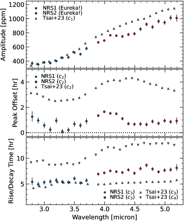
Figure 11. Phase-curve amplitude (c1, top panel), peak offset measured with respect to periapse (c2 − tper, middle panel), and rise/decay timescale (c3/c4, bottom panel) derived from the NRS1 and NRS2 data using the nominal (symmetric) model (blue circles and red squares, respectively) compared with those derived from the GCMs published by S.-M. Tsai et al. (2023b; white triangles). The GCM phase curves are highly asymmetric and were therefore fit using the asymmetric model that includes both c3 (the rise timescale) and c4 (the decay timescale).
Download figure:
Standard image High-resolution imageUnlike for the observed NRS1 and NRS2 phase curves, the GCM phase curves are highly asymmetric and exhibit much longer decay timescales. This is evident in Figure 12, which shows brightness temperatures associated with the integrated NRS1 and NRS2 best-fitting phase curves. A shorter observed rise/decay timescale may indicate that HD 80606 b has a shorter radiative timescale and/or a shorter rotation period than that associated with the GCM predictions published by S.-M. Tsai et al. (2023b). A rotation period that is shorter than the assumed ≈40 hr pseudo-synchronous rotation period (i.e., a higher apparent wind speed; P. Hut 1981) will result in more of the planet’s cooler side becoming visible toward the end of the observing window, causing a more rapid cooling rate to be inferred.
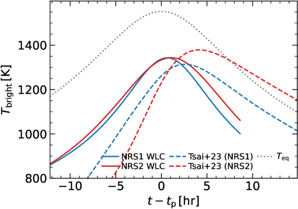
Figure 12. Brightness temperatures calculated from the best-fitting NRS1 and NRS2 phase curves (solid blue and red, respectively) compared with phase curves calculated using the GCMs published by S.-M. Tsai et al. (2023b) over the same NRS1/NRS2 bandpasses. The dotted black line shows the instantaneous irradiation temperature calculated assuming full heat redistribution and zero albedo.
Download figure:
Standard image High-resolution imageThe more rapid decrease in flux relative to the S.-M. Tsai et al. (2023b) cloud-free GCM predictions may also be due to the advection of nightside clouds onto the dayside during the postperiapse phases, which would cause the observed flux to be suppressed. This scenario was proposed by J. de Wit et al. (2016) and N. K. Lewis et al. (2017) to explain the low brightness temperatures derived from HD 80606 b’s Spitzer 4.5 μm phase curve. As noted in Section 4.1.2, the rate at which the Spitzer 4.5 μm flux rises during the preperiapse phase is consistent with the NRS2 white-light light curve, while the postperiapse decrease in flux is notably slower compared to NRS2. This could be caused by differences in the distribution of the advected clouds between the two observing epochs.
Based on our analysis, HD 80606 b’s emission spectrum appears to transition from one that is initially indistinguishable from a blackbody to one that exhibits detectable molecular absorption features of H2O, CO, and CH4. It is plausible that this transition is caused by the rapid evaporation of clouds near the photosphere, which may block flux emitted from below the cloud deck. This scenario is consistent with the fact that the transition occurs when the photospheric temperature near 10 mbar increases to ∼1200 K, coinciding with the condensation point of MnS clouds (C. V. Morley et al. 2012). Along with MgSiO3 and Na2S, MnS was previously identified as a potentially significant condensate in HD 80606 b’s atmosphere using GCMs postprocessed to include clouds (N. K. Lewis et al. 2017).
5.3. Temperature Structure
Ignoring the potential impact of clouds on the observed emission spectral features, the transition from a blackbody spectrum preperiapse may simply be caused by a change in the temperature gradient near the photosphere. In this case, a (nearly) isothermal PT profile will produce weak or nonexistent absorption/emission features. We find that the derived PT profiles at all phases exhibit relatively low temperature gradients near the photosphere and we do not find clear evidence of a temperature inversion near the IR photosphere. This stems from the lack of obvious emission features appearing in any of the extracted emission spectra. The GCM-based predictions from S.-M. Tsai et al. (2023b) show a transient inversion forming near the IR photosphere that persists throughout the 21 hr observing window, which leads to the formation of subtle but detectable emission features (e.g., Figure 16). N. Iro & L. D. Deming (2010), N. K. Lewis et al. (2017), and L. C. Mayorga et al. (2021) make similar predictions based on 1D radiative transfer models, 3D GCMs, and 1D radiative-convective equilibrium models, respectively.
5.4. Chemical Composition
The atmospheric retrievals that we carried out for the four postperiapse phases that deviate significantly from a blackbody spectrum imply that HD 80606 b’s atmosphere has an approximately solar metallicity with [M/H] = −0.17 ± 0.31—slightly below the host-star metallicity of 0.348 ± 0.057 (L. J. Rosenthal et al. 2021)—and a solar C/O = 0.49 ± 0.15. We might expect that, as the planet approaches its host star, CH4 is converted into CO through thermochemical reactions in response to the increase in temperature within the atmosphere (see Figure 8 showing the derived PT profiles compared with the expected points along which CH4 and CO are in equal abundance); however, in the case of HD 80606 b, these reactions are expected to occur over timescales much longer than the orbital timescale (N. Iro & L. D. Deming 2010; C. Visscher 2012; S.-M. Tsai et al. 2023b). The photochemical models generated for HD 80606 b by S.-M. Tsai et al. (2023b) predict that the abundances of CH4, H2O, and CO undergo significant changes in response to the increase in incident UV flux that occurs during periapse passage. The resulting change in CH4 and CO abundances, along with that of several photochemical by-products such as C2H2 and HCN, can differ by orders of magnitude from chemical-equilibrium predictions that neglect photochemistry.
Using both detectors without including a flux offset, we find that CH4 is detected in all four of the extracted postperiapse emission spectra, while CO and H2O are detected during two and three phases, respectively. We find that both the chemical-equilibrium and free retrievals yield high-quality fits, and that the latter models are statistically preferred due to the fewer number of free parameters. This suggests that the atmosphere is not strongly impacted by disequilibrium chemistry or photochemistry. Water is not detected during the first postperiapse phase, which results in a significantly supersolar C/O = 0.74 ± 0.015 and [M/H] = 1.24 ± 0.65, and a 2σ upper limit of the volume mixing ratio (VMR) of  being inferred from the free retrieval. While this may be evidence of disequilibrium chemistry, it is ambiguous due to the fact that it is only associated with a single phase and may be related to the pre/postperiapse transition from a blackbody spectrum. Ultimately, a more sophisticated modeling framework that can better capture shorter-timescale variability and/or 3D effects may provide improved constraints on potential changes in the atmosphere’s chemical composition.
6. Conclusions
We present the first partial phase-curve observations of an exoplanet obtained with JWST. These NIRSpec/G395H measurements of HD 80606 b’s periapse passage reveal an atmosphere that undergoes significant temperature changes during the 21 hr observing window. This work demonstrates that partial phase curves with JWST can provide reliable data at twice the photon noise precision level. Time-dependent spectral changes in the NIRSpec/G395H bandpass are observed in the emission spectrum of the planet during this observation. Our analysis suggests that, prior to periapse, the atmospheric layers probed at these wavelengths are predominantly isothermal based on the fact that no spectral features are detected and the derived planet spectrum is consistent with that of a blackbody. During the postperiapse phases, we detect CH4, H2O, and CO spectral absorption features with maximum significance levels of 10.7σ, 5.5σ, and 4.4σ, respectively, when considering both the NRS1 and NRS2 detectors without including a flux offset parameter for NRS1. When including a flux offset, CH4 and CO are the only species detected at 5.7σ and 3.8σ, respectively, while considering only the NRS2 detector yields a 3.6σ detection of CO. We find that the postperiapse emission spectra are generally consistent with thermochemical-equilibrium models, and therefore the atmosphere appears to be chemically mixed. No significant spectral emission features are detected at any of the observed phases, which, along with the PT profiles derived from atmospheric retrievals, rules out the presence of a predicted temperature inversion (N. Iro & L. D. Deming 2010; N. K. Lewis et al. 2017; L. C. Mayorga et al. 2021; S.-M. Tsai et al. 2023b).
Considering the significantly higher precision of JWST NIRSpec observations relative to the Spitzer 4.5 μm and 8 μm partial phase curves, additional measurements extending over a longer time span may be capable of detecting a ringing effect caused by the planet’s rotation/advection (N. B. Cowan & E. Agol 2011; T. Kataria et al. 2013; M. Vanrespaille et al. 2024). This would provide important and entirely unique constraints that are needed to accurately model the atmospheres of eccentric hot Jupiters like HD 80606 b and hot Jupiters in general. Additional phase-curve measurements of HD 80606 b obtained at different wavelengths will also help to constrain the chemical and photochemical reactions that are likely occurring in the atmosphere. For example, by incorporating HST WFC3/G141 measurements and/or JWST NIRISS/SOSS or NIRSpec/G140M measurements, we gain sensitivity to gaseous H2O (S. Constantinou et al. 2023; B. Benneke et al. 2024), which, similar to CH4, is predicted to decrease in abundance with increasing CO due to photochemical reactions (S.-M. Tsai et al. 2023a). Moreover, partial phase curves obtained at longer wavelengths using instruments like MIRI/LRS can provide insight into the composition and size of cloud particulates (e.g., the observed flux ≳20 hr postperiapse is predicted to be significantly higher if MnS clouds are present compared to MgSiO3 clouds; N. K. Lewis et al. 2017). High-resolution near-IR observations have the potential to detect HCN (e.g., S. Gandhi et al. 2020; A. Sánchez-López et al. 2022) that is expected to be found at high altitudes in hot Jupiter atmospheres (e.g., R. Baeyens et al. 2024). Therefore, future high-precision observations of HD 80606 b and other eccentric hot Jupiters such as HAT-P-2 b (N. K. Lewis et al. 2013), HD 17156 b (T. Kataria et al. 2013), and XO-3 b (L. Dang et al. 2022) using JWST or ground-based high-resolution spectrographs may provide important clues into the nature of hot Jupiter atmospheres and the impact of photochemistry and clouds.
Acknowledgments
J.T.S. and J.L. acknowledge support from NSF AAG award AST2009343. J.T.S. acknowledges funding support from grant 22JWGO1-17 awarded by the CSA. This work is based on observations made with the NASA/ESA/CSA James Webb Space Telescope. The data were obtained from the Mikulski Archive for Space Telescopes at the Space Telescope Science Institute, which is operated by the Association of Universities for Research in Astronomy, Inc., under NASA contract NAS5-03127 for JWST. These observations are associated with program #2488. K.D.C. acknowledges support for program #2488 was provided through a grant from the STScI under NASA contract NAS5-03127. J.M.D. acknowledges support from the Amsterdam Academic Alliance (AAA) Program, and the European Research Council (ERC) European Union’s Horizon 2020 research and innovation program (grant agreement no. 679633; Exo-Atmos). This work is part of the research program VIDI New Frontiers in Exoplanetary Climatology with project number 614.001.601, which is (partly) financed by the Dutch Research Council (NWO). L.D. acknowledges support from the Banting Postdoctoral Fellowship program, administered by the Government of Canada and the Trottier Family Foundation.
We thank Everett Schlawin, Shang-Min Tsai, and Maria Steinrueck for helpful discussions that improved the analysis of the data and the interpretation of the results presented in this work.
All the JWST data used in this paper can be found in MAST: doi:10.17909/yb30-hj11.
Facilities: JWST - James Webb Space Telescope (NIRSpec).
Software: AstroPy (Astropy Collaboration et al. 2013, 2018, 2022), matplotlib (J. D. Hunter 2007), numpy (C. R. Harris et al. 2020), scipy (P. Virtanen et al. 2020), petitRADTRANS (P. Mollière et al. 2019), Eureka! (T. Bell et al. 2022), jwst, batman (L. Kreidberg 2015), emcee (D. Foreman-Mackey et al. 2013, 2019), easyCHEM (P. Mollière et al. 2017), PyratBay (P. E. Cubillos & J. Blecic 2021).
Appendix
The Allan deviation plots for the white and spectral light curves are shown in Figure 13 and the marginalized posterior distributions for the NRS1 white-light curve is shown in Figure 14. The emission spectra (planet-to-star flux contrast) derived for all ten phases are shown in Figure 15. Figure 16 shows the marginalized posterior distribution associated with the petitRADTRANS-based retrieval obtained for a single phase and additional retrieval results are presented in Figure 17. Additional plots presenting the chemical equilibrium retrieval results are shown in Figure 18 where we also include the chemical abundances associated with the forward models.
S. E. Moran et al. (2023) show that the two NIRSpec/G395H transit observations of GJ486 b (GO-1981; PI: Stevenson) exhibit strong, wavelength-dependent slopes similar to what we find in our analysis of the NRS1 measurements of HD 80606 b. This is evident when comparing the 2D spectra shown in our Figure 2 with Figure 1 of S. E. Moran et al. (2023). Here we present a more quantitative comparison between the linear and quadratic trends associated with both NRS1 data sets.
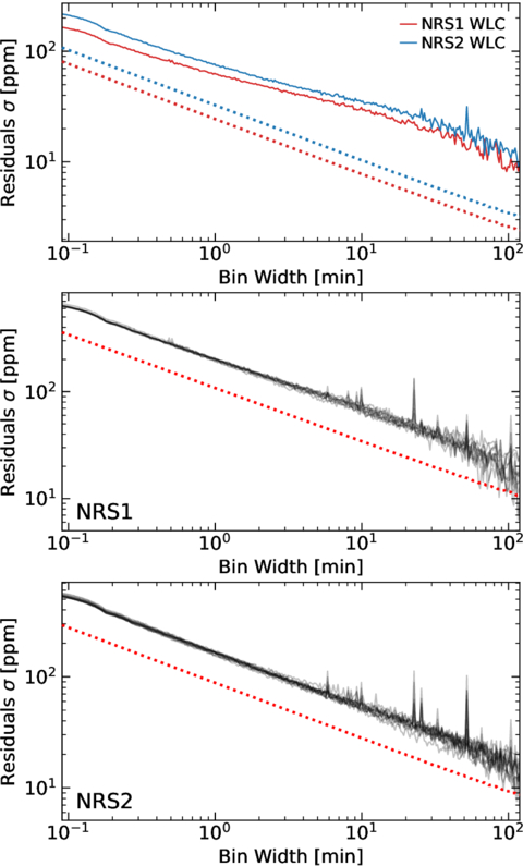
Figure 13. Top: Allan deviation plots for the NRS1 (solid blue) and NRS2 (solid red) white-light light curves. Dashed lines correspond to the expectations from pure photon noise (81 ppm for NRS1 and 108 ppm for NRS2); the unbinned light curves have a scatter of 2.03× and 2.02× the photon noise. Middle and bottom: Allan deviation plots for the 10 NRS1 spectral light curves and the 14 NRS2 spectral light curves normalized to the values associated with the first wavelength channel in order to compare across all channels. The spectral light curves have a scatter of 1.71–1.94× each channel’s photon noise.
Download figure:
Standard image High-resolution image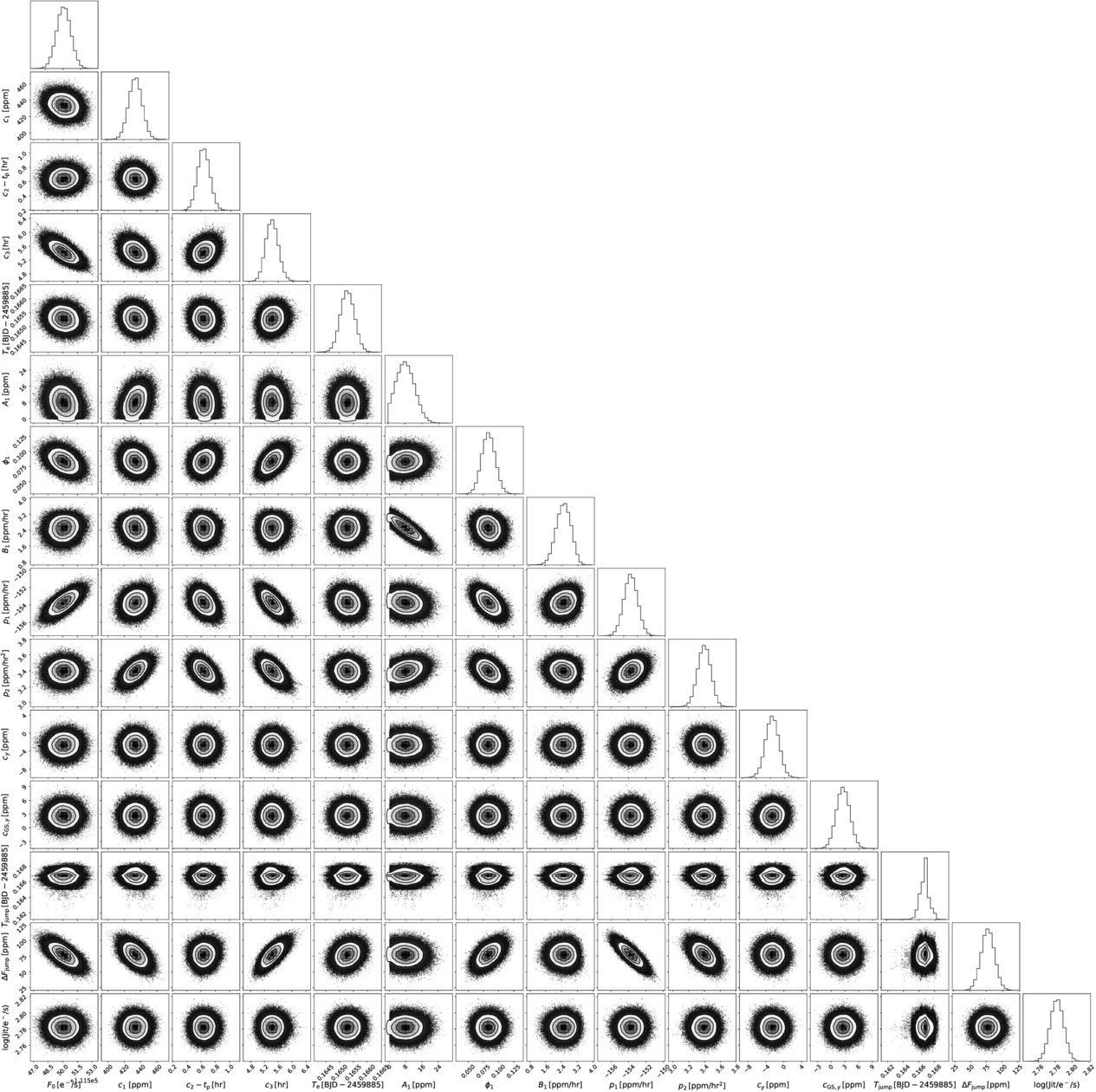
Figure 14. Marginalized posterior distributions for the NRS1 white-light light curve using the nominal model.
Download figure:
Standard image High-resolution imageWe reduced the NRS1 G395H time-series observations for the first of two transit observations of GJ486 b using essentially the same Eureka! control files used for the HD 80606 b data. We used an aperture half-width of 5 pixels rather than 4 (as adopted for the HD 80606 reduction) to match what was used by S. E. Moran et al. (2023). We also manually masked nine columns (i.e., wavelength channel light curves) that were identified by eye as having anomalous flux values. We then extracted the white-light curve and 10 spectral light curves and fit a 2nd-order polynomial to each light curve’s out-of-transit baseline measurements. The baseline fit to the white-light light curve is shown in Figure 15; the residuals for this baseline fit have a 153 ppm scatter, which is comparable to the 132–158 ppm scatter obtained by S. E. Moran et al. (2023) for the same data set using Eureka!, FIREFLy (Z. Rustamkulov et al. 2022), and Tiberius (J. Kirk et al. 2018, 2021) reduction pipelines.
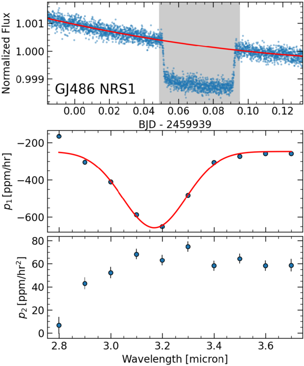
Figure 15. Out-of-transit baseline fit to the first of two publicly available NRS1 transit observations of GJ486 b, which was obtained using NIRSpec/G395H with three groups. The top panel shows the white-light light curve with the associated 2nd-order polynomial baseline model (red); the out-of-transit measurements (blue points outside the gray box) have residuals with a 153 ppm scatter. The middle and bottom panels show the linear (p1) and quadratic (p2) baseline polynomial terms derived from the spectral light curves. The red curve in the middle panel is a Gaussian fit used for comparison with the similar trend found in the HD 80606 NRS1 observation.
Download figure:
Standard image High-resolution image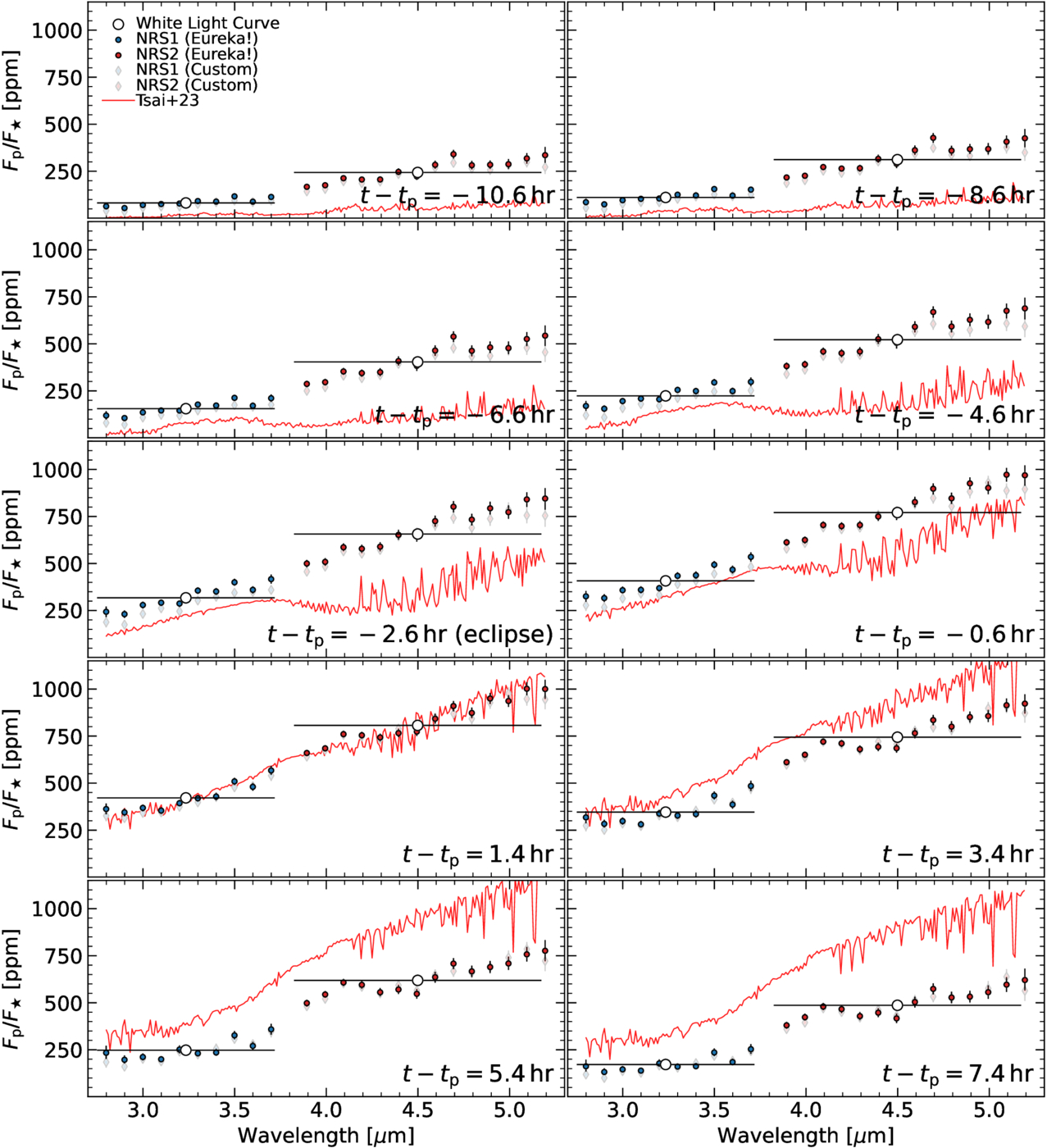
Figure 16. Planet-to-star flux contrast derived using the NRS1 and NRS2 light-curve models for the Eureka! reduction (dark circles) and the custom reduction (light diamonds). Red lines show the model spectra published by S.-M. Tsai et al. (2023b) after applying instrumental broadening and binning for visual clarity.
Download figure:
Standard image High-resolution image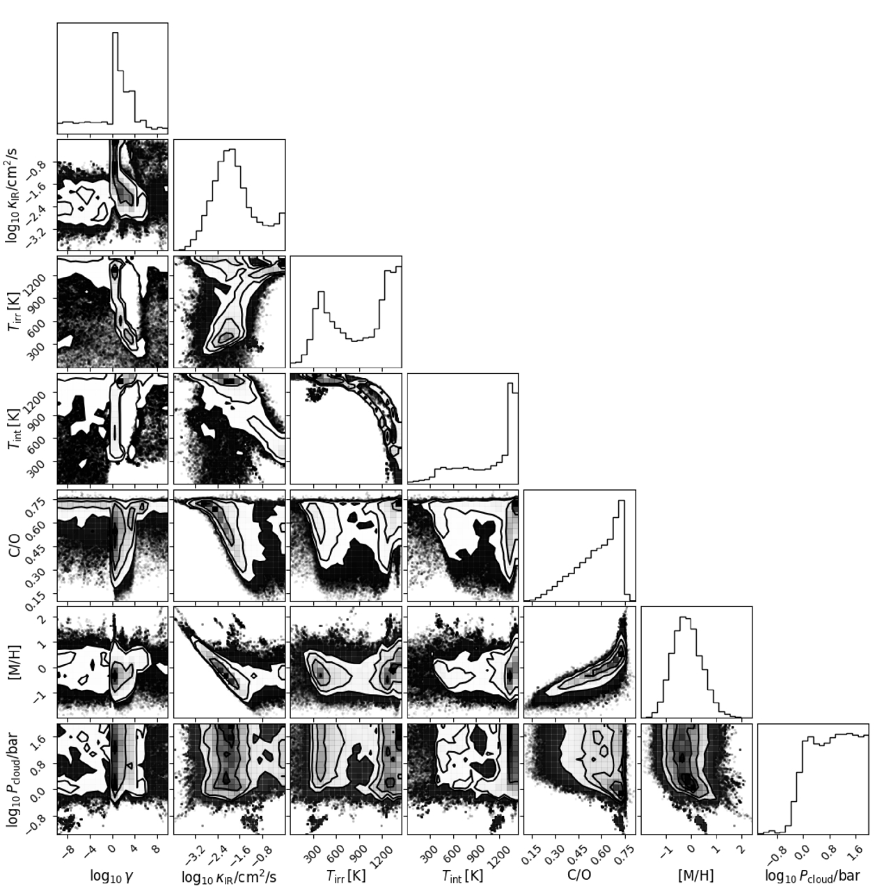
Figure 17. Marginalized posteriors derived for the chemical-equilibrium retrieval for the t − tp = 3.4 hr phase shown in Figure 8.
Download figure:
Standard image High-resolution image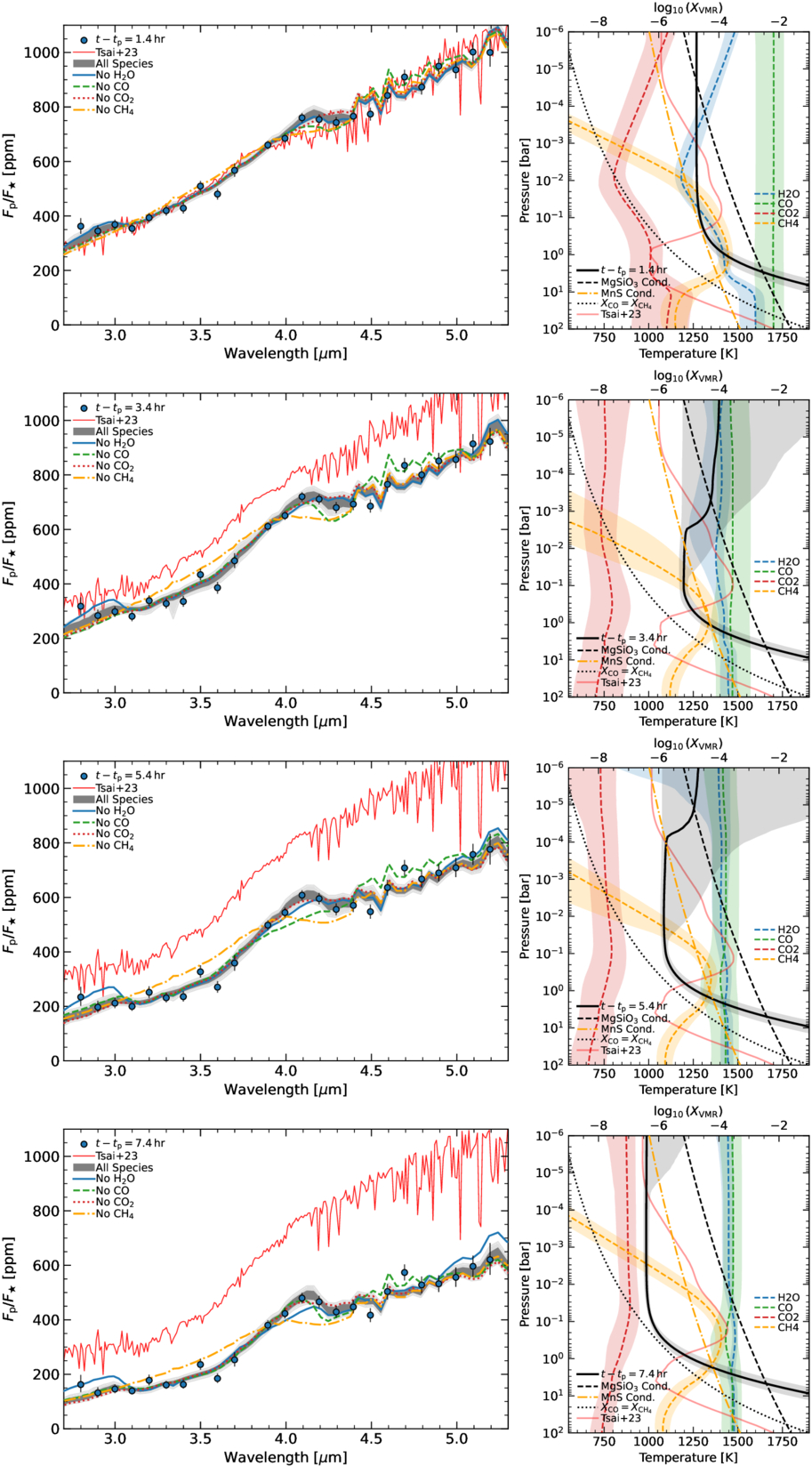
Figure 18. Chemical-equilibrium retrieval results (similar to Figure 8) for the last four phases where the PT profiles include the H2O, CO, CO2, and CH4 abundances plotted as VMRs along the top axis. All colored contours correspond to 1σ.
Download figure:
Standard image High-resolution imageThe polynomial coefficients, p1 and p2, derived from the GJ486 NRS1 spectral light curves are shown in the bottom two panels of Figure 15. We find that the p1(λ) values show a similar Gaussian-like trend as that obtained for HD 80606’s NRS1 data set, with minimum values occurring at the 3.2 μm wavelength bin. The GJ486 results show a p2(λ) that is essentially constant for λ ≥ 3.1 μm and which decreases for the 3λ < 3.1 μm bins. We note that the GJ486 baseline is likely impacted by stellar activity/starspots, which, along with the different instrument setups, prevent a one-to-one comparison with the HD 80606 polynomial coefficients from being carried out.