Abstract
Stellar light curves from edge-on double white dwarf (DWD) systems have periodic lensing/eclipsing signals at times of alignment between the two components as seen by the observer. Here, we study the characterization and detection of these signals. In common DWDs, the Einstein radii have similar orders of magnitude to the radii of the white dwarfs (WDs), and the projected source and lens radii normalized to the Einstein radius (ρ⋆ and ρl) are ∼1. Both of them are reduced with the orbital period and the lens mass. If ρl ≃ 1 the lensing-induced minor image is always blocked by the lens, which results in lower magnification factors. If ρl ≲ 1, and in transit events, the finite-lens effects decrease the light curves’ width. When ρl ≳ 1 (which happens for close DWDs consisting of a low-mass WD and a massive one) deep or complete eclipses dominate over lensing effects. The self-lensing signals are maximal for massive DWDs in wide orbits. We study the detectability of lensing/eclipsing signals in edge-on DWDs in observations by NASA’s Transiting Exoplanet Survey Satellite (TESS), the Vera Rubin Observatory Large Synoptic Survey Telescope (LSST), and the Nancy Grace Roman Space Telescope. We simulate stellar light curves due to edge-on DWDs and generate synthetic data points based on their observing strategies. Detection efficiency is maximal for extremely low-mass WDs in close orbits, and the numbers of DWDs within 100 pc and an observing cone with detectable lensing/eclipsing signals in one observing window of 27.4 days for TESS and 62 days for Roman are ∼1 and <1, respectively. Detecting these signals by LSST is barely possible because of its long cadence.
Original content from this work may be used under the terms of the Creative Commons Attribution 4.0 licence. Any further distribution of this work must maintain attribution to the author(s) and the title of the work, journal citation and DOI.
1. Introduction
Evolutionary tracks of different stars reveal that stars with initial masses lower than 8 M⊙ will evolve to white dwarfs (WDs). WDs are compact objects with masses in the range ∼[0.17−1.4] M⊙ and average radii ∼0.01 R⊙, which decrease with increasing mass (see, e.g., M. Nauenberg 1972; F. Ambrosino 2020). Galactic models predict that around ten billion WDs live in our Galaxy, and 9%–14% of these are double WDs (DWDs; S. Toonen et al. 2017). However, in some other references the predicted binarity fraction for WDs in our galaxy is ≲1% (e.g., G. Nelemans et al. 2001). DWD systems are mainly generated from binary stars. The separations of WDs in such systems are predicted to be lower than their initial separations, because when the lower-mass stellar companion is in the red giant phase and overfills its Roche lobe, mass transfer occurs and as a result their separation is reduced.
There are several methods to create binarity of WDs, depending on their orbital periods, orbital inclination angles, and surface temperatures. These methods can be classified into (i) spectroscopic manifestation from either radial velocities (through periodic variations of the location of strong absorption lines) or their double-lined overlapped luminosity (see, e.g., M. Kilic et al. 2020a), and (ii) photometric observations to capture either periodic eclipsing or self-lensing signals (N. Garza Navarro & D. J. Wilson 2021; J. Munday et al. 2023; H.-M. Jin et al. 2025). However, in close DWDs some other photometric variations could occur such as Doppler boosting (A. Shporer et al. 2010). Nowadays, there are several telescopes and facilities that are able to capture these signals, such as Gaia, NASA’s Transiting Exoplanet Survey Satellite (TESS; G. R. Ricker et al. 2014), the Vera C. Robin Observatory, which was named the Large Synoptic Survey Telescope (LSST; LSST Science Collaboration et al. 2009), the Zwicky Transient Facility (E. C. Bellm et al. 2019), etc. (see, e.g., G. Nir & J. S. Bloom 2025; S. Sajadian & N. Afshordi 2024).
Close DWD systems, with short orbital periods from several hours to minutes, are very interesting targets because they are potential sources of low-frequency gravitational waves detectable by space-based interferometers such as the Laser Interferometer Space Antenna (P. Amaro-Seoane et al. 2017), TianQin (J. Luo et al. 2016), and Taiji (W.-H. Ruan et al. 2020). In addition, they are progenitors of Type Ia supernovae. PTF J0533+0209 is an example of a close DWD system with an orbital period of 20 minutes; it consists of a CO WD and an extremely low-mass (ELM) He WD (K. B. Burdge et al. 2019). The formation of this target is under debate, e.g., H.-L. Chen et al. (2022) discussed that this target has not likely formed through common-envelope (CE) evolution.
Two potential channels exist for the formation of close DWDs. In the first channel a donor star is rotating around a CO WD in a close orbit, so that stable mass transfer occurs between them. Such systems are converted to DWDs consisting of a CO WD and an He WD. For such systems there is a correlation between He WD mass and the orbital period (T. M. Tauris & G. J. Savonije 1999). Through this mechanism, ELM WDs can be born (Z. Li et al. 2019; L. T. T. Soethe & S. O. Kepler 2021). There is another mechanism that produces close DWD systems, in which a CO WD and a red giant have a CE with unstable mass transfer. Then and after ejecting the CE, a DWD system (CO WD and He WD) will form.
Most DWDs discovered up to now are close and have short orbital periods. For instance, W. R. Brown et al. (2020) found 98 DWDs through the ELM spectroscopic Survey (W. R. Brown et al. 2010) while all targets had orbital periods shorter than 1.5 days. Also, J. Munday et al. (2024) found 34 DWD systems with double-line signatures in their spectra with orbital periods shorter than 13.5 days. The main reason for this is that detecting interacting binaries is easier than detecting detached ones, although there should be more detached binaries than interacting ones. For instance, B. Willems & U. Kolb (2004) showed that wide and noninteracting binaries including WDs generally would comprise more than 75% of all binary systems containing WDs. If detached DWDs are edge-on as seen by the observer, we can realize their binarity by capturing either their self-lensing or eclipsing signals.
In this paper, we study the characterization and detection of gravitational self-lensing signals reduced by eclipse in edge-on DWDs. Self-lensing happens in binary systems include compact objects whose orbital plane is edge-on as seen by the observer (A. Maeder 1973; G. Wiktorowicz et al. 2021; S. Sajadian & N. Afshordi 2024). During self-lensing signals due to compact objects some part of the images’ area will be blocked by the compact object’s disk, which is the so-called finite-lens effect or occultation or eclipse (see, e.g., E. Agol 2002). Finite-lens effects decrease or even remove the self-lensing signals, while they are not recognizable from lensing signals in real observations (C. Han 2016; S. Sajadian & H. Fatheddin 2025). The probability of self-lensing signals occurring in binary systems was first estimated by A. Gould (1995) and B. Qin et al. (1997). G. M. Beskin & A. V. Tuntsov (2002) roughly estimated the number of self-lensing signals that can be detected by the Sloan Digital Sky Survey (SDSS, D. G. York et al. 2000) due to different binary systems including compact objects by analytically evaluating probability functions. Based on the same method, G. Nir & J. S. Bloom (2025) roughly evaluated the number of detectable self-lensing signals in edge-on binary systems that can be detected by the new generation of ground- and space-based telescopes, such as the Vera C. Robin observatory, TESS telescope, etc. Up to now, several self-lensing signals due to binary systems including WDs and main-sequence stars have been discovered through the Kepler and TESS data (E. Kruse & E. Agol 2014; H. Kawahara et al. 2018; K. Masuda et al. 2019; N. M. Sorabella et al. 2024).
The outline of the paper is as follows. We explain our formalism to simulate these systems and their self-lensing/eclipsing signals in Section 2. Additionally, in this section we evaluate the lensing parameters, and lensing/eclipsing signals in all possible DWD systems. In Section 3, we numerically calculate self-lensing/eclipsing light curves using the inverse-ray-shooting (IRS) method and discuss their properties. In Section 4, we investigate the detectability of these signals through three observing strategies by the TESS, LSST, and Roman telescopes. Finally, we conclude and review the results in Section 5.
2. Lensing/Eclipsing Signals in Edge-on DWD Systems
We explained our method for simulating binary systems including compact objects and stellar companions and creating their self-lensing and eclipsing signals in detail in S. Sajadian & N. Afshordi (2024) and S. Sajadian (2014). Here, to simulate DWD systems and their light curves we use the same method, and we review it here briefly. To simulate a binary system consisting of two WDs, we consider some parameters: their masses (M1 and M2), their surface temperatures (Teff,1 and Teff,2), their orbital period T, and the orbital eccentricity . We determine the radii of the WDs using the known mass–radius relationship for WDs as given by M. Nauenberg (1972). Also, Kepler’s third law indicates the semimajor axis of their orbit a.
To project their orbital planes on the sky plane, generally two projection angles are necessary: (i) one, θ, to project the minor (or major) axis of the orbital plane on the sky plane and (ii) another, the so-called inclination angle i, to project the orbital plane normal to the sky plane and on the line of sight toward the observer.
The self-lensing signals occur when the two components of the binary system are collinear (their projected separation on the sky plane is minimum) as seen by the observer. In DWD systems, both components are luminous and compact, so that two self-lensing signals occur during one orbital period, and they are not necessarily similar. For each self-lensing signal the foreground WD is the lens object with mass and radius Ml and Rl, and the farther WD is the source object, whose mass and radius are specified by M⋆ and R⋆, respectively.
The self-lensing formalism is similar to the microlensing one, in which we have a characteristic length, the so-called Einstein radius (the radius of the images’ ring at the time of complete alignment), given by

where G is the gravitational constant, c is the speed of light, and Dl and Ds are the lens and source distances from the observer, respectively. Also, Dls = Ds − Dl is the lens–source separation in the line-of-sight direction. We note that for binary systems Dl ≃ Ds and Dls ≃ a. Accordingly, in DWD binary systems the three lengths Rl, Rs, and RE have similar orders of magnitude.
In DWD systems, the magnification factor suffers from two effects: the finite source size and the finite lens size. The finite source size is evaluated from ρ⋆, which is the source radius projected on the lens plane and normalized to the Einstein radius as given by

The magnification factor is calculated by considering the finite source size, which was first done by H. J. Witt & S. Mao (1994):
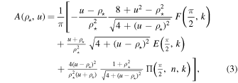
where u is the lens–source separation projected on the lens plane and normalized to the Einstein radius,  , and
, and  . Also, the functions F, E, and Π are the first, second, and third types of the elliptical integral, respectively. For extremely large source sizes (ρ⋆ ≫ 1) and when the lens is crossing the source disk the magnification factor is estimated as
  and does not depend on u (A. Maeder 1973; A. Gould & C. Gaucherel 1996; E. Agol 2003; S. Sajadian 2023). Generally, enhancing the finite source size decreases the magnification factor and generates a more flattened light curve. We calculate the magnification factor during self-lensing signals and by considering the finite source size and a limb-darkened profile for the source surface brightness, A(ρ⋆, u, Γ), using the public code VBBinaryLensing (V. Bozza 2010; V. Bozza et al. 2018). Here, Γ is the linear limb-darkening coefficient.
The finite lens size is evaluated from the normalized lens radius, which is

The finite-lens effect reduces the magnification factor because the lens’s disk blocks some parts of the images’ area. We show the occultation due to the finite-lens effect by  , which is the ratio of the area of the image that is covered by the lens’s disk to the source area (when both of them are projected on the lens plane) and calculate it numerically using the IRS method (see, e.g., J. Wambsganss 1998; S. Sajadian & S. Rahvar 2010). This factor is given by

where the integration is done over the images’ area (I) projected on the lens plane and specified with (x, y),  is the distance of a given point on the images’ area from the lens position (which is at the center of the coordinate system), and Θ is a step function, which is one if R ≤ Rl and zero otherwise. f(x, y, Γ) is the surface brightness over the images’ disk at the position (x, y). Also, R⋆,p = R⋆Dl/Ds is the source radius projected on the lens plane.
The fraction of the images’ area covered by the lens disk is given by  . If
. If  the images are completely covered by the lens and a complete eclipse happens. The overall normalized fluxes in lensing signals by the first and second WD are (respectively)

where  is the ratio of the first WD’s flux to the second WD’s flux.
In Figure 1, we show the maps of RE(0.01 R⊙), ρ⋆, and ρl over the 2D space Ml(M⊙)–M⋆(M⊙) due to different DWD systems in three panels. The ranges of lens and source masses are [0.17, 1.4] M⊙ with 100 grids over each axis. We fix their orbital periods to 10 days, the system distance from the observer to 1 kpc, and the orbital eccentricity to zero for these maps. To find the effect of the orbital period on these maps, we make them for a wide range of orbital period T ∈ [1, 50] days, and the animation from the resulting maps versus T is available.
Figure 1. Maps of RE(0.01 R⊙), ρ⋆, and ρl over the 2D space Ml(M⊙)–M⋆(M⊙) due to different DWD systems. For these maps, two parameters are fixed: the orbital period T = 10 days and the system distance from the observer Dl = 1 kpc, and we assume their orbits are circular. To understand the effect of the orbital period on these maps, an animation of the maps of RE, ρ⋆, and ρl vs. orbital period is available. The animation shows the evolution from T = 1–50 days. The real-time duration of the animation is 50 s.
(An animation of this figure is available.)
Download figure:
Video Standard image High-resolution imageAccording to these figures, ρl values depend strongly on the lens object as well as the orbital period, and do not significantly depend on source stars. For massive WDs, e.g., Ml ≳ 1.3 M⊙, ρl ∼ 0.3−0.4 even for a wide range of the orbital period, so we do not expect significant eclipsing effects. When lens and source objects are low-mass ones with M ≲ 0.3 M⊙, ρ⋆ and ρl are as large as ≳3, so no self-lensing signal occurs, and a complete eclipse for short orbital periods will happen. In contrast, DWD systems consisting of two massive WDs with masses greater than a solar mass have ρl ≲ 1 and ρ⋆ ≲ 1, which offer self-lensing signals without eclipsing.
In Figure 2, we show the maps of the magnification factor A, the fraction of the images’ area covered by the lens object  , and
, and  , which is the relative residual (the ratio of the residual area between the images and the source star to the source’s area) over the 2D space Ml(M⊙)–M⋆(M⊙) and by considering two values for the lens–source separation normalized to the Einstein radius, u = 10−4ρ⋆ (top panels) and u = 3.5ρ⋆ (bottom panels). Here some parameters are fixed: T = 10 days, Γ = 0.45, and Dl = 1 kpc. However, for other orbital periods in the range T ∈ [1, 50] days we make these maps and the animation from them available.
Figure 2. Maps of the magnification factor A, the fraction of the images’ area covered by the lens object  , and
, and  , which is the relative residual in the normalized flux due to both self-lensing and occultation signals over the 2D space Ml(M⊙)–M⋆(M⊙). Over these maps the contour lines of ρ⋆ (left panel), ρl/ρin and ρl/ρout (middle panel), and ρlρ⋆ (right panel) are shown. For these maps some parameters are fixed: T = 10 days, Dl = 1 kpc, and Γ = 0.45, and the lens–source separation normalized to the Einstein radius is u = 10−4ρ⋆ (top panels) and u = 3.5ρ⋆ (bottom panels). To study the effect of the orbital period on these maps, for T ∈ [1, 50] days we generate these maps and an animation from the maps of A,
  , and δ, which is available. The animation shows the T = 1–50 days sequence for the u = 0.0001 panels. The real-time duration of the animation is 50 s.
(An animation of this figure is available.)
Download figure:
Video Standard image High-resolution imageHere, the relative residual will be positive, i.e., δ > 0, when the normalized flux of the source star (the ratio of the images’ flux received by the observer to the stellar flux at the baseline) is greater than one. If the normalized flux of the source star is less than one, then δ < 0. The minimum value of δ is −1, which occurs when the images’ disk is completely covered by the lens’s area, i.e.,  . Also, δ = 0 occurs when there are no net lensing/eclipsing signals for the source star. In addition, over the map of magnification factor the contour lines of ρ⋆ are plotted as dashed black curves. The magnification factor in DWD systems due to massive WDs is as high as 10 or even more, because for these systems ρ⋆ is quite small and ∼0.1.
When the lens is crossing the source disk (u0 < ρ⋆), the fraction of the images’ disk that is covered by the lens  can be evaluated by comparing the inner and outer radii of the images’ ring (Rin and Rout) and the lens radius. Here, u0 is the lens impact parameter, which is the minimum lens–source separation projected on the lens plane and normalized to the Einstein radius. The inner and outer radii of the images’ ring normalized to the Einstein radius (when ρ⋆ is not small) are given by
  and
and  , respectively. If ρl > ρout a complete eclipse occurs, and when ρl < ρin no eclipse happens. Between these two limits (i.e., ρin ≤ ρl ≤ ρout) a partial eclipse occurs.
Hence, over the map of  (the top middle map in Figure 2) the contour lines of ρl/ρout and ρl/ρin are plotted with dashed black and dotted–dashed red curves, respectively. For ρl > ρout, a complete eclipse happens, i.e.,
  (yellow parts). Accordingly, in transit events when Ml ≲ 0.3 M⊙ complete eclipses occur, and for Ml ≳ 1.0 M⊙ no eclipse happens.
The magnification factor and eclipsing signals depend on ρ⋆ and ρl, respectively, so that when both of them are reduced, self-lensing and eclipses are enhanced and decreased, respectively. Hence, on the map of the relative residual δ we show the contour lines of ρl × ρ⋆, whose value reduces with the orbital period and the masses of both the source and lens WDs. Hence, DWDs consisting of two massive WDs in wide orbits have the highest magnification factors, and DWDs consisting of one ELM WD (as the lens object) and one massive WD (as the source star) in close orbits have the deepest or complete eclipsing signals (−1 ≤ δ ≤ 0).
In the bottom panels of Figure 2, we show similar maps for a larger lens–source separation (normalized to the Einstein radius) u = 3.5ρ⋆ in which the lens does not cross the source’s disk. The magnification factor can reach 2 when both the lens and source WDs are massive. The complete eclipse happens only when an ELM WD is the lens object and orbiting a very massive WD (the source star). We do not plot the contour lines ρl/ρin and ρl/ρout over the middle maps, because for this u value the ring of images is not generated. In the next section, we simulate several light curves due to different edge-on DWD systems and discuss their properties.
3. Light Curves of Edge-on DWD Systems
Based on the formalism introduced in the previous section, we generate light curves due to different DWD systems numerically. In Figure 3, six examples of these light curves are displayed. In each panel, three curves are plotted that show the self-lensing signal (dashed green curve), eclipse by the lens disk (solid red curve), and the overall lensing/eclipsing signal (dotted–dashed black curve) versus time. Also, some key parameters can be found at the top of each panel. For Γ (linear limb-darkening coefficient of the source brightness profile), ρ⋆, and ρl, u0/ρ⋆ two values are given, which are due to the signals on the left and right respectively. In these panels, the signals that are specified with dark colors (dark red and dark green for eclipsing and self-lensing signals) happen when M1 is the lens object and M2 is the source star as labeled with Lens: M1. Hence, the darker signal is scaled with  , and the other is scaled with
  (see Equation (6)). We note that
  is the ratio of the flux of the WD with mass M1 to the flux of the WD with mass M2 at the baseline. All light curves are simulated for the time interval [0, T] days, but the horizontal axes do not represent the full time interval of the orbital period. Instead they show two zoomed time intervals around the lensing/eclipsing signals. For each light curve shown in one panel of Figure 3, we show the map of its lensing-induced images’ surface brightness at a given time (which is specified with a dotted blue line on that light curve) in the corresponding panel of Figure 4. In each panel of this figure, three circles are shown, which are the source’ edge projected on the lens plane (white circle), the lens’s edge (black circle), and the Einstein ring (dashed red circle). The axes are normalized to the source radius projected on the lens plane (R⋆,p). For each panel, an animation from similar maps versus time is available.
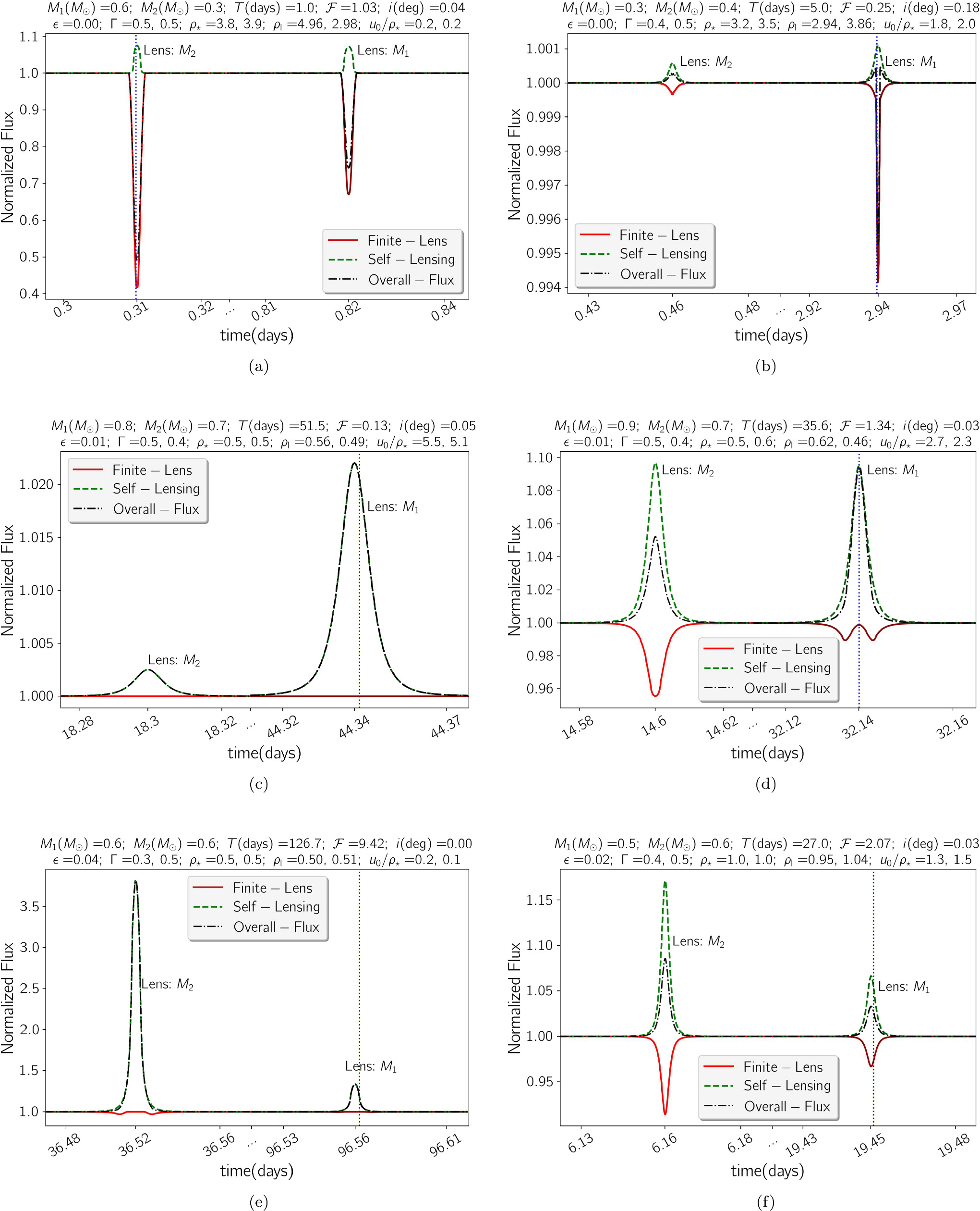
Figure 3. Six examples of light curves due to different edge-on DWD systems are presented in different panels. In each panel, three curves are shown, which are the normalized fluxes by considering self-lensing (dashed green), eclipse by the lens disk (solid red), and both of them (dotted–dashed black) vs. time. At the top of each panel, some key parameters are mentioned. For Γ, ρ⋆, ρl, and u0/ρ⋆ two values are given, which are due to the signals on the left and right respectively. The lensing/eclipsing signals due to the lens object with mass M1 are specified with dark green and dark red colors and labeled with it. The horizontal axes show two zoomed time intervals around lensing/eclipsing signals. The dotted blue lines determine the times at which their corresponding images’ surface brightnesses are shown in Figure 4.
Download figure:
Standard image High-resolution image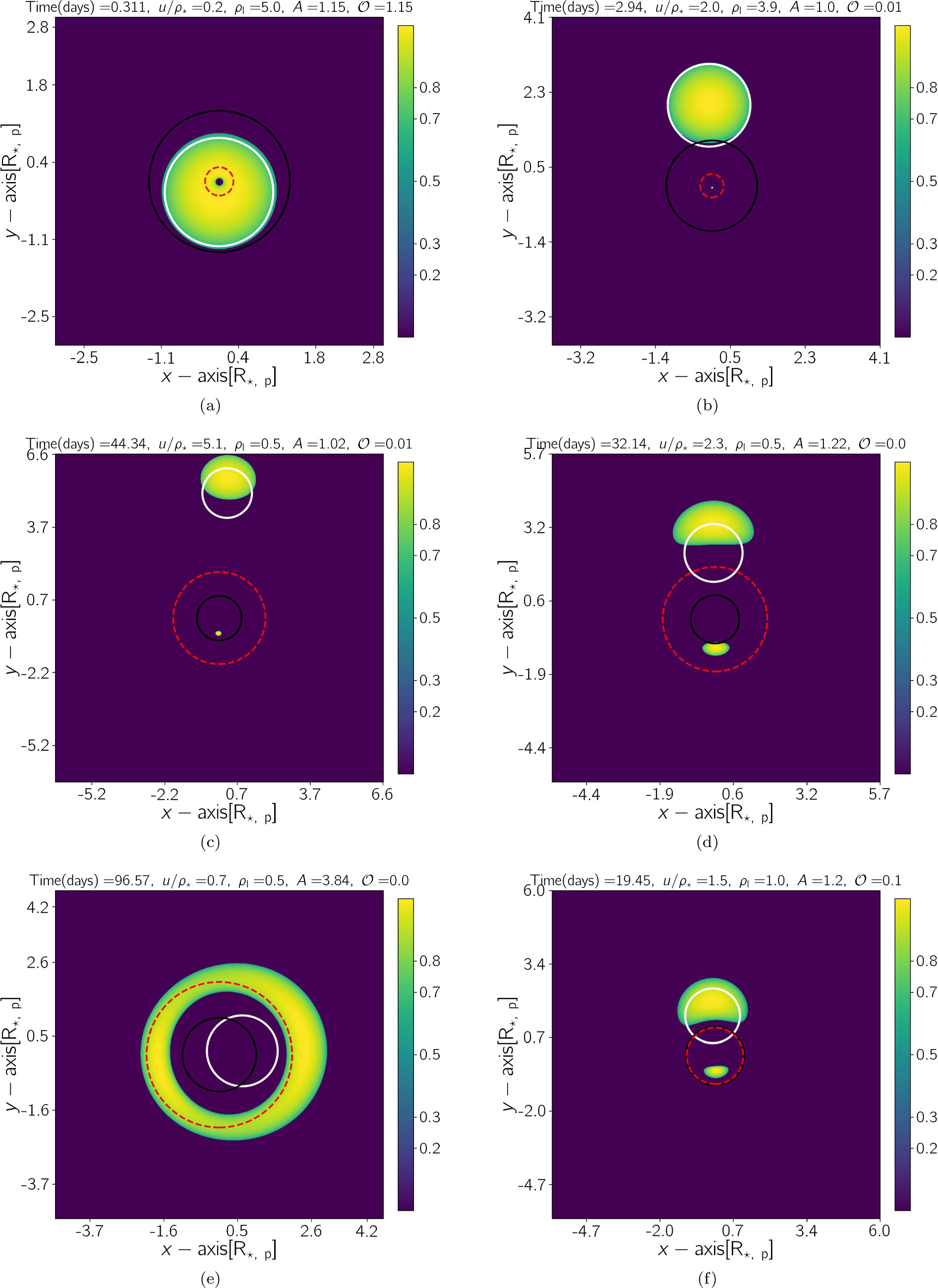
Figure 4. Each panel shows the lens plane for each light curve in Figure 3 at the time specified with a dotted vertical line on that light curve. In each panel, the map determines the lensing-induced images’ surface brightness. The white, black, and dashed red circles specify the source star’s edge, the lens’s edge, and the Einstein ring, respectively. For each panel some relevant parameters are mentioned at the top. The axes are normalized to the source radius projected on the lens plane R⋆,p = R⋆Dl/Ds. For each light curve, we make create maps vs. time, and six animations from these maps related to the light curves in Figures 3(a)–(f) are available.
Download figure:
Standard image High-resolution imageIn Figure 3(a), one of the WDs has a low mass, i.e., 0.3 M⊙. When its companion WD is collinear with such a low-mass lens object as seen by the observer a complete eclipse occurs (the first signal with ρl = 5). However, since ρ⋆ ≃ 3.8 the lensing effect is negligible and a thick ring of images will form that is similar to the source star. We show a map of the lensing-induced images’ surface brightness (by considering a linear limb-darkening profile for the source star) on the lens plane at the specified time (with a blue vertical line) in Figure 4(a). For this system and during the second alignment between the lens and source stars ρ⋆ > ρl and the lens impact parameter is smaller than the source radius, so the eclipse happens only for some part of the images’ disk.
In the second panel, Figure 3(b), a light curve due to an edge-on DWD is represented with one eclipse and one self-lensing event. Generally, in microlensing (or self-lensing) events when u0 > ρ⋆ two images are formed, one inside the Einstein ring (the so-called minor image) and the other outside (the major image). Here and during both alignments, u0 > ρ⋆ and two images form. Considering ρl values, minor images and some part of the major images are blocked by the lens disk. However, in the first signal, the lensing-induced shear of the major image is considerable, which causes a small eclipse, in contrast to the second signal. The map of images at the given time during the second signal is shown in Figure 4(b).
As mentioned in the previous section, the light curves due to edge-on DWD systems consisting of more massive WDs show self-lensing with either small or negligible eclipse effects. However, in these systems the resulting light curves depend strongly on the lens impact parameter. In Figures 3(c), (d), and (e) we show the light curves due to massive DWD systems by considering three different lens impact parameters.
In Figure 3(c), the light curve represents two self-lensing signals without considerable eclipsing effects. During both signals u0 ≳ 2.5(ρ⋆ + ρl), which means only minor images are blocked. To show this situation, we represent the images’ map projected on the lens plane in Figure 4(c) at the time of 44.34 days. Accordingly the minor image is much smaller than the major image, because of the large lens impact parameter. In this light curve, the binary orbit is almost circular so the lensing parameters for the two signals are similar, although the ratio of the first signal to the second signal is  .
.
In Figure 3(d), another light curve is plotted. In this system, ρ⋆ ∼ 0.5, similar to the previous light curve, but its lens impact parameters are smaller (in comparison with the previous light curve), which results in larger minor images and greater occultation effects. The occultation effects in the two signals are different. In the first signal, the minor image is blocked by the lens during lensing, whereas in the second signal the minor image is not blocked by the lens disk around the time of closest approach, because it moves out of the lens disk. We show this situation (the images’ map) in Figure 4(d). For the second signal the overall flux versus time is narrower (although its peak does not change) because of the occultation effect.
In Figure 3(e), the stellar light curve due to an edge-on DWD system consisting of two similar WDs (with different surface temperatures) is shown. For this target, u0 < ρ⋆ which means the lens is crossing the source disk. Therefore, for this target whenever u < ρ⋆ the images will form a thick ring around the Einstein ring. Since ρl ≃ 0.5, the images’ ring is out of the lens disk and no occultation occurs. Hence, for transit events and while the lens is crossing the source disk, there is no occultation effect as long as ρl ≲ ρin. We show the images’ ring in Figure 4(e).
In the last panel, Figure 3(f), we display a light curve due to a common DWD system with the WDs’ mass ∼0.5–0.6 M⊙. For this target ρ⋆ ≃ 1 and ρl ≃ 1. Since u0 > ρ⋆, no ring of images forms and instead minor and major images are formed inside and outside the Einstein ring. Since ρl ≃ 1, the minor image is always blocked by the lens’s disk. Hence, for such events (which are common), the lensing and occultation curves are similar. The overall normalized flux versus time is a lensing-like (and symmetric) curve. The images’ map due to this target at the time of closest approach is shown in Figure 4(f).
4. Detectability of Lensing/Eclipsing Signals from DWD Systems
In this section, we first perform Monte Carlo simulations from DWD systems, and generate their light curves as detailed in Section 4.1. Then, in Sections 4.2, 4.3, and 4.4 for generated light curves we simulate synthetic data points taken by the TESS, LSST, and Roman telescopes, extract the light curves with detectable lensing/eclipsing signals, and evaluate their statistics and properties.
4.1. Monte Carlo Simulations from DWD Systems
WDs in our simulations are chosen from a big sample consisting of 1772 WDs within 100 pc, which were discovered from SDSS observations (M. Kilic et al. 2020b). We determine their absolute magnitudes in the TESS T band, the LSST filters, and the Roman W149 filter based on their relations with absolute magnitudes in the Gaia bands, i.e., G, GRP, and GBP (A. U. Landolt 2009; S. Alam et al. 2015; K. G. Stassun et al. 2018). We note that the magnitude in the W149 filter is one third of the sum of absolute magnitudes in the standard filters H, J, and K (B. T. Montet et al. 2017; S. Sajadian & A. Salehi 2020). For a DWD system we need two WDs to produce a binary system. Their semimajor axis is selected from Öpik’s law, i.e., a log-uniform distribution and from the range a ∈ [3R⋆, 105R⋆]. However, we exclude interacting systems in which their Roche lobe distances (B. Paczyński 1971) are less than the source radii. The eccentricity is chosen uniformly from the range ![$\epsilon \in [0,{\epsilon }_{\max}]$](https://content.cld.iop.org/journals/1538-3881/169/3/164/revision1/ajadab74ieqn24.gif) , where
, where  is given by the known period–eccentricity correlation for binary systems (T. Mazeh 2008). We limit the inclination angle to i ∈ [0°, 5°] to simulate edge-on binary systems. The projection angle θ is chosen uniformly from the range [0°, 360°].
We numerically calculate the finite-lens effect and the factor  using the IRS method. However, to speed up these calculations and create a large sample of all possible light curves due to different DWD systems, we improve our previous method, which was explained in S. Sajadian & H. Fatheddin (2025). In lensing events due to single lens objects the two generated images have the same azimuth angles with the source star, so in any step we rotate the coordinate system and set the source star on the right side of the horizontal axis (x-axis) at the normalized distance u from the lens object, i.e., x⋆ = u, y⋆ = 0. We know that in a lensing event due to a single lens object two images are formed such that the minor image is always inside the Einstein ring and the major image is close to the source position. Hence, for any given u we search a rectangular part of the lens plane with the ranges
 ![$x\in \left[\right.{x}_{1},{x}_{2}\left]\right.$](https://content.cld.iop.org/journals/1538-3881/169/3/164/revision1/ajadab74ieqn27.gif) and
and ![$y\in [0,1+2.5{\rho }_{\star }]$](https://content.cld.iop.org/journals/1538-3881/169/3/164/revision1/ajadab74ieqn28.gif) , where
, where

However, this area covers half of the images, and the resulted  should be doubled. In the IRS method, we divide the Einstein radius into 200 grids.
After simulating synthetic data points and to extract detectable events, we apply four criteria as follows. (i) SNR > 3: the signal-to-noise ratio (SNR) should be greater than 3. Here,  , where ΔF is the maximum lensing/eclipsing-induced depth in the normalized flux, and Ntran = Tobs/T is the number of transits during the observing time Tobs.
  is the photometric error in the normalized flux, and σm is the photometric error in the stellar apparent magnitude. (ii) Ntran ≥ 1, which guarantees that at least one lensing/eclipsing signal happens during the observing time. (iii) ΔF ≥ 2σF, which means that the depth should be greater than 2σF. (iv) Δt ≥ τ, where Δt is the duration of lensing/eclipsing signals and τ is the observing cadence, which is 2 minutes for the TESS Candidate Target List (CTL) observations. The last two criteria are complementary and reject some light curves with either very short or shallow signals, although they could have reasonable SNR values.
We perform three Monte Carlo simulations from these DWDs so that they are adjusted for potential observations by the TESS, LSST, and Roman telescopes. Their details and results are illustrated in the following subsections.
4.2. Detectable DWDs in the TESS Observations
In the first Monte Carlo simulation for potential observations of DWD systems by the TESS telescope we set DWD systems at the real distances (reported from the SDSS observations) of their first components. In this simulation, we simulate synthetic data points during 27.4 days with two one-day gaps after each observing time window of 12.4 days. We note that more than 70% of the TESS targets are observed during only 27.4 days every two years (i.e., more than 70% of stars in each hemisphere are covered only by one TESS sector). We assume that these targets are in the TESS CTL (K. G. Stassun et al. 2018) and are observed with a 2 minutes cadence. More details of simulating the TESS observations can be found in S. Sajadian et al. (2024) and S. Sajadian & N. Afshordi (2024). The photometric error in the TESS observation is an increasing function of stellar apparent magnitude and their relation is shown in Figure 1 of S. Sajadian et al. (2024). Also, the combined differential photometric precision (J. L. Christiansen et al. 2012) is a known metric that shows the photometric precision in normalized flux reported by the Kepler and TESS telescopes.
Four examples of simulated light curves with generated synthetic data points are presented in Figure 5. The structures of these plots are similar to those shown in Figure 3. The magenta data points represent the synthetic data points taken by the TESS telescope. At the top of each plot, the parameters to evaluate their detectability are mentioned. For these parameters the two values given relate to the first and second signals. For the first light curve, Δt/τ = 0.7 and no data points cover its signals, although its second signal is relatively deep with a high SNR value (30 as mentioned in the legend). In the second panel of Figure 5 one light curve is shown, which is also not detectable because its signals have similar depths to the photometric errors ΔF/σF = 1.6 and 0.8. The two bottom panels display two detectable light curves.
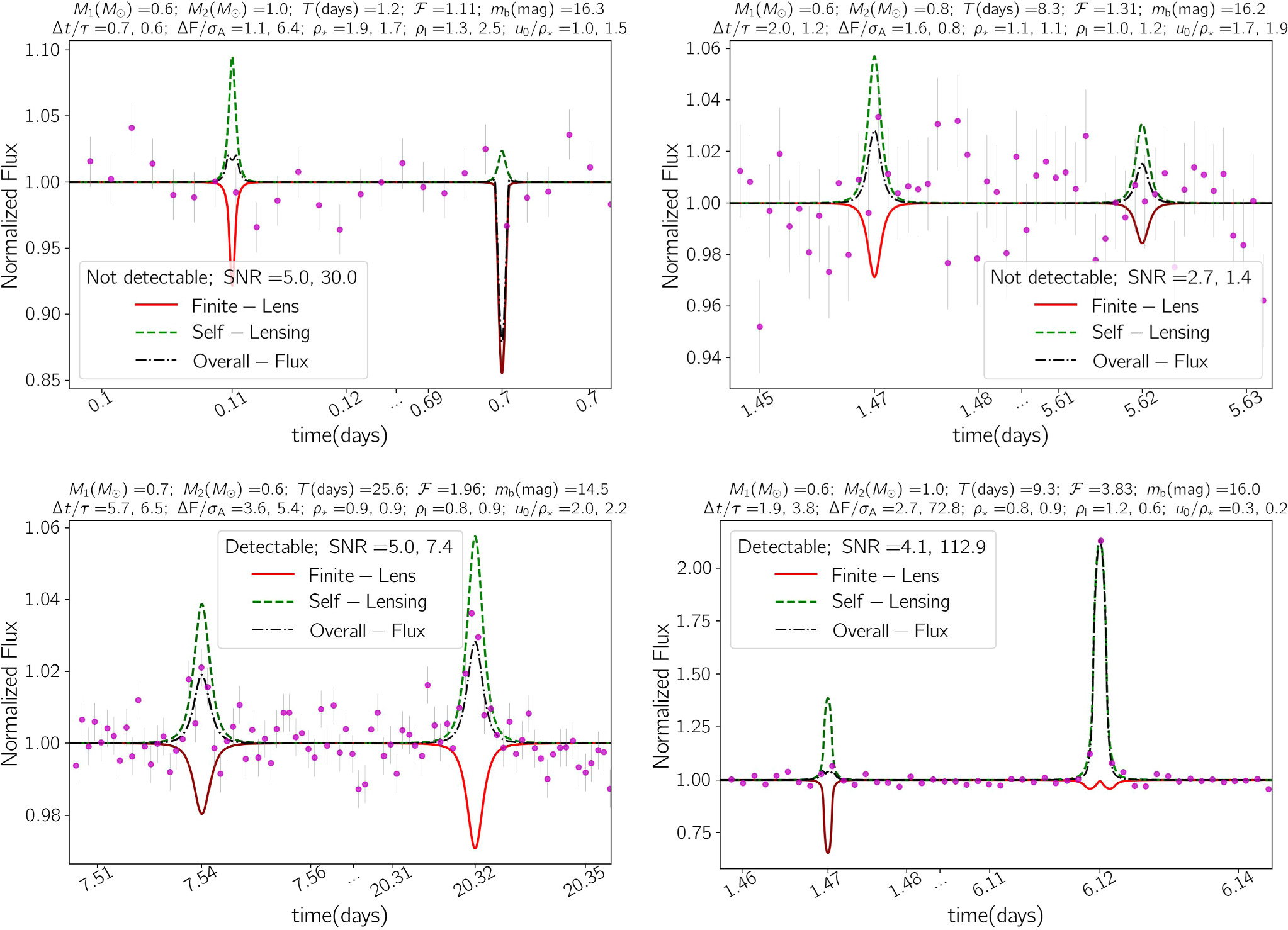
Figure 5. Four examples of simulated light curves due to edge-on DWD systems with the synthetic data points generated based on the TESS observing strategy with a 2 minutes cadence. Some physical and characteristic parameters of these light curves are mentioned above the panels. For some parameters the two values given relate to the first and second signals, respectively.
Download figure:
Standard image High-resolution imageIn the first Monte Carlo simulation related to the TESS observations, we generate light curves and synthetic data points for events with 0.8 ≤ T(days) ≤ 27.4 and mbase ≤ 17.5 mag. These events have Ntran ≥ 1 and could be detectable in the TESS photometric system. Here, ![${m}_{{\rm{base}}}\,=-2.5{\mathrm{log}}_{10}\left[\right.1{0}^{-0.4{m}_{{\rm{l}}}}+1{0}^{-0.4{m}_{\star }}\left]\right.+2.5{\mathrm{log}}_{10}[{f}_{{\rm{b}}}]$](https://content.cld.iop.org/journals/1538-3881/169/3/164/revision1/ajadab74ieqn32.gif) is the baseline apparent magnitude in the TESS T band due to the DWD system and blending stars. Therefore, ml and m⋆ are the apparent magnitudes of the lens and source WDs in the TESS T band. Here, for all targets, we set the blending factor fb = 1 because WDs are relatively close to the observer.
is the baseline apparent magnitude in the TESS T band due to the DWD system and blending stars. Therefore, ml and m⋆ are the apparent magnitudes of the lens and source WDs in the TESS T band. Here, for all targets, we set the blending factor fb = 1 because WDs are relatively close to the observer.
According to simulations, ε1 = 25.3% of all simulated events have 0.8≤ T(days) ≤ 27.4 and mbase ≤ 17.5 mag. The TESS efficiency to detect periodic lensing/eclipsing signals in edge-on DWDs with baseline magnitude in the T band less than 17.5 mag and orbital period T ∈ [0.8, 27.4] days is ε2 = 1.53%. The probability that stellar orbits have inclination angles less than 5° (edge-on orbits) is ε3 = 5.6%. If we assume that the WDs are uniformly distributed in our Galaxy and 14% of them are in binary systems, then in a spherical volume of radius 100 pc around the Sun there should be ∼4,350 DWD systems. And ∼244 of these systems are edge-on with i ≤ 5°, one of which will have detectable lensing/eclipsing signals. However, the TESS telescope can detect farther and fainter WDs systems through its full-frame images. Also some of the TESS CTL targets are detected for more than 27.4 days because of some overlapping sectors. Therefore, the real number of DWD systems with detectable signals in the TESS observations should be higher.
To study the properties of detectable events, three scatter plots from simulated events are presented in Figure 6. In the top panel, all events with simulated light curves are shown with black circles over the 2D space Ml(M⊙)–M⋆(M⊙), with two marginal and normalized 1D distributions (gray ones). The DWD systems with detectable self-lensing or eclipsing signals are specified with blue and green stars, respectively. The normalized distributions due to all detectable events are shown in magenta. Over the marginal distributions the TESS detection efficiencies versus given parameters are offered with black step lines. The detection efficiency for a given parameter is the ratio of the number of DWD systems with that given parameter and detectable signals to the total number of simulated ones with the given parameter. The first panel shows that although most WDs have mass ∼0.6 M⊙, the detection efficiency is higher for other WD masses. However, the detection efficiency for lower masses (≲0.4 M⊙, for most of which complete eclipses happen) is higher than that for higher masses.
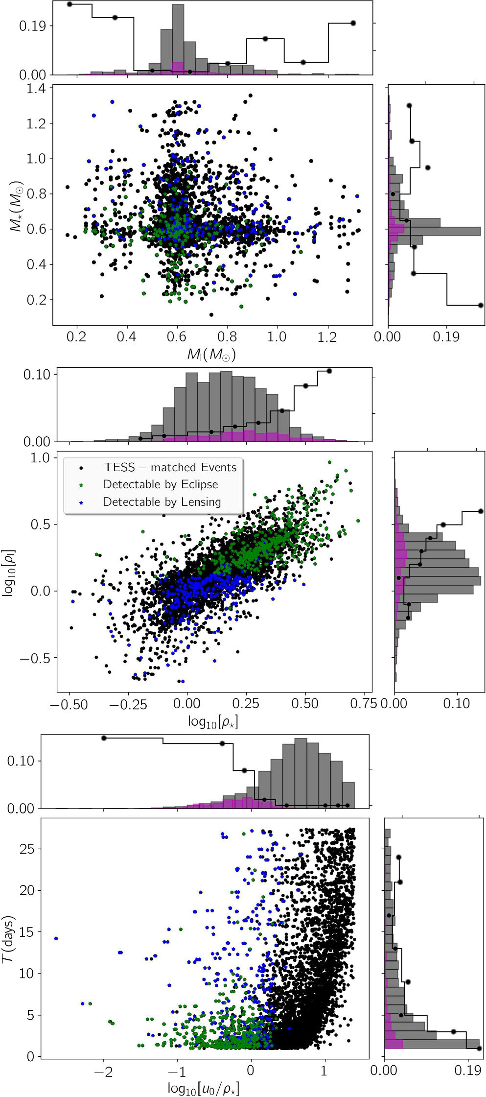
Figure 6. Scatter plots of all simulated DWD systems (black circles) over three 2D spaces Ml(M⊙)–M⋆(M⊙) (top panel), ![${\mathrm{log}}_{10}[{\rho }_{\star }]-{\mathrm{log}}_{10}[{\rho }_{{\rm{l}}}]$](https://content.cld.iop.org/journals/1538-3881/169/3/164/revision1/ajadab74ieqn33.gif) (middle panel), and
(middle panel), and ![${\mathrm{log}}_{10}[{u}_{0}/{\rho }_{\star }]-T({\rm{days}})$](https://content.cld.iop.org/journals/1538-3881/169/3/164/revision1/ajadab74ieqn34.gif) (bottom panel), with two marginal and normalized distributions. Over each plot, the targets with detectable self-lensing and eclipsing signals in the TESS observations are specified with blue and green stars, and their normalized distributions are shown in magenta. Also, we plot the detection efficiencies over the marginal parts with black step lines. We note that in the last two plots there are twice as many entries because each simulated light curve has two signals.
(bottom panel), with two marginal and normalized distributions. Over each plot, the targets with detectable self-lensing and eclipsing signals in the TESS observations are specified with blue and green stars, and their normalized distributions are shown in magenta. Also, we plot the detection efficiencies over the marginal parts with black step lines. We note that in the last two plots there are twice as many entries because each simulated light curve has two signals.
Download figure:
Standard image High-resolution imageIn the middle panel of Figure 6 we show a similar scatter plot but over the 2D space ![${\mathrm{log}}_{10}[{\rho }_{\star }]-{\mathrm{log}}_{10}[{\rho }_{{\rm{l}}}]$](https://content.cld.iop.org/journals/1538-3881/169/3/164/revision1/ajadab74ieqn35.gif) . We note that this panel and the bottom one have twice as many entries as the top panel, because every light curve has two signals. The detection efficiency is higher for systems with large ρ⋆ and ρl values, while most of them have eclipsing signals (especially the events with ρl ≳ 1). Such systems have short orbital periods (higher Ntran values). The DWD systems with small ρ⋆ and ρl values are mostly detectable due to their self-lensing signals although their detection efficiency is small.
. We note that this panel and the bottom one have twice as many entries as the top panel, because every light curve has two signals. The detection efficiency is higher for systems with large ρ⋆ and ρl values, while most of them have eclipsing signals (especially the events with ρl ≳ 1). Such systems have short orbital periods (higher Ntran values). The DWD systems with small ρ⋆ and ρl values are mostly detectable due to their self-lensing signals although their detection efficiency is small.
In the bottom panel we show a similar scatter plot but over the 2D space ![${\mathrm{log}}_{10}[{u}_{0}/{\rho }_{\star }]-T({\rm{days}})$](https://content.cld.iop.org/journals/1538-3881/169/3/164/revision1/ajadab74ieqn36.gif) . Most DWD systems with u0 ≲ ρ⋆ have detectable signals. The systems with longer orbital periods have self-lensing signals rather than eclipsing ones. Generally, closer systems (with shorter orbital periods) have higher detection efficiencies. Hence, the detection efficiency for edge-on DWD systems depends significantly on (i) orbital period, (ii) the lens impact parameters, and (iii) the total mass of the system, so that close and ELM ones with smaller inclination angles are the most favorable with deep or even complete eclipsing signals.
. Most DWD systems with u0 ≲ ρ⋆ have detectable signals. The systems with longer orbital periods have self-lensing signals rather than eclipsing ones. Generally, closer systems (with shorter orbital periods) have higher detection efficiencies. Hence, the detection efficiency for edge-on DWD systems depends significantly on (i) orbital period, (ii) the lens impact parameters, and (iii) the total mass of the system, so that close and ELM ones with smaller inclination angles are the most favorable with deep or even complete eclipsing signals.
4.3. Statistics of Detectable DWDs in the LSST Observations
The observing cadence of the LSST telescope is not short enough to capture lensing/eclipsing signals in edge-on DWD systems, although its observing time window is predicted to be 10 years. To show this point, we evaluate the duration of lensing/eclipsing signals, i.e., Δt ∼ 2RWD/v, to find the longest one and study whether it is realizable in the LSST data. Here, v = 2πa/T is the relative velocity in a circular binary orbit. We consider DWD systems with very long orbital periods T ∼ 10 yr (which is the LSST observing time span), which have semimajor axis a ∼ 105RWD. Accordingly, the duration of their lensing/eclipsing signals would be ∼15 minutes, where we use RWD ∼ 0.01 R⊙. Such short signals cannot be captured in the LSST observations, whose cadence is 3 days. We note that the duration of lensing signals with small ρ⋆ values is longer and is proportional to the time of crossing the Einstein radius, the so-called Einstein crossing time tE = RE/v ∼ 1−1.5 hr. This time is also considerably shorter than the LSST cadence. So it seems that there is no hope that this telescope can detect lensing/eclipsing signals from DWD systems, even detached ones with long orbital periods.
4.4. Statistics of Detectable DWDs in the Roman Observations
We also evaluate the detectability of these signals during the Roman observations toward the Galactic bulge. This telescope will detect the Galactic bulge continuously for 62 days with a 15 minutes cadence. Its cadence and observing time span are relatively suitable for detecting lensing/eclipsing signals due to DWD systems. This telescope will detect a small part of the sky toward the Galactic bulge (∼2 deg2).
Discerning isolated DWD systems at great distances is not possible (because of their faintness). For instance, a typical WD in the Galactic bulge has an average apparent magnitude ∼28 mag in the Roman filter W149. Considering the size of the stellar point-spread function (PSF) in the Roman observations, which is  , the average number of blending stars whose light enters a stellar PSF toward the Galactic bulge is ∼3–9. Although, by adding the blending and background light to a DWD system in the Galactic bulge it will be detectable in the Roman observation, the blending effect decreases the lensing/eclipsing signals significantly so that the resulting signals are not detectable. Hence, in the simulation we limit the distance of WDs to D = 5 kpc from the observer and perform a similar Monte Carlo simulation. Many details for Roman-based simulations can be found in the previous papers (S. Sajadian 2021; S. Sajadian & K. C. Sahu 2023).
In the simulation we create light curves for the events with T ∈ [1, 62] days, and mbase ∈ [14.8, 26] mag in the Roman filter W149, which constitute ε1 = 14.84% of all simulated events with distance less than 5 kpc. For these events, we generate synthetic data points as taken by the Roman telescope and apply four mentioned detectability criteria to extract the detectable events. Only ε2 = 0.07% of these events passed the criteria and had detectable lensing/eclipsing signals. To estimate the number of DWDs that this telescope can detect, we find the number of DWD systems inside a cone of height h = 5 kpc and angular area dΩ = 2 deg2 (its radius is R ≃ 70 pc). This number can be estimated as where VR = πR2h/3 is the volume of the cone from our location toward the Galactic bulgewith height 5 kpc and radius R, and V ≃ 1350 kpc3 is the total volume of our Galaxy. Considering that only 0.56% of these systems are edge-on with inclination angle less than 5°, we conclude that the number of edge-on DWD systems with detectable lensing/eclipsing signals in the Roman observations is ∼0.1, which is less than one.
5. Conclusions
It has been predicted that 10 billion WDs exist in our Galaxy and ∼9%−14% of them are double (e.g., see S. Toonen et al. 2017). DWDs are interesting systems because they are progenitors of Type Ia supernovae and low-frequency gravitational waves. Detecting these systems has commonly been (and is) done through spectroscopic measurements, either of their radial velocities or by detecting their overlapping spectra (see, e.g., W. R. Brown et al. 2020; J. Munday et al. 2024). If DWD systems are edge-on as seen by the observer some periodic lensing or eclipsing signals occur in their light curves and one can study them through dense and accurate photometric observations. In this work, we studied the characterization and detection of these lensing/eclipsing signals.
For common DWD systems three lengths—the Einstein radius and the source and lens radii—are of the same order of magnitude (∼0.01 R⊙), which means that the source and lens radii normalized to the Einstein radius (ρ⋆ and ρl) are mainly close to one. We considered all possible values for the mass of WDs (i.e., [0.17, 1.4]M⊙) and a wide range for the orbital period of T ∈ [1, 50] days, and found self-lensing signals in DWD systems enhanced with the orbital period and the masses of source and lens objects. For example, the magnification factors in edge-on DWD systems consisting of massive WDs with T ∼ 1, 20 days can reach ∼6, 17, respectively. Deep or even complete eclipsing signals will occur if the lens is an ELM WD. For instance, in most transit events (u < ρ⋆) when Ml ≲ 0.3 M⊙ complete eclipsing signals occur (see middle panels of Figure 2). Generally, the overall normalized flux has the strongest lensing-like signals for DWD systems with two massive WDs in wide orbits and the deepest or complete eclipsing signals when DWD systems consist of one massive and one low-mass WD in a close orbit so that the low-mass one is the lens object.
For edge-on DWD systems with ρl ∼ 1, the lens object blocks the minor images at times, which results a more flattened light curve (normalized flux owing to both lensing and eclipsing effects versus time). When ρl < 1, the occultation of the minor image will not happen at the time of closest approach and the resulting light curve will be narrower whereas its peak does not change because of the finite-lens effect. When ρl is larger than one, the eclipse effect is considerable and for  a complete eclipse occurs.
We also studied the detectability of lensing/eclipsing signals due to DWD systems in TESS, LSST, and Roman observations. By performing Monte Carlo simulations from these light curves and generating synthetic data points, we concluded that the detection efficiency for lensing/eclipsing signals from edge-on DWD systems depends significantly on (i) orbital period, (ii) the lens impact parameters, and (iii) the mass of the lens object, so that close and ELM lenses with smaller inclination angles are the most favorable ones with deep or even complete eclipsing signals.
Inside a sphere around the Sun of radius 100 pc there are ∼4350 DWD systems, 244 of which are edge-on as seen by the observer (i ≤ 5∘). Of these edge-on DWD systems, 62 have orbital periods in the range [0.8, 27.4] days and are brighter than 17.5 mag in the TESS T band. According to our simulations, one of these systems (closer than 100 pc from us) has detectable lensing/eclipsing signals in the TESS observations during a 27.4 day observing window and with a 2 minutes cadence.
We also evaluated their detectability by the Vera C. Robin observatory and concluded that its cadence is too long to cover such short lensing/eclipsing signals, even for DWD systems with orbital periods as long as 10 years.
Another observation in near future with a cadence suitable for detecting these signals will be made with the Roman space telescope toward the Galactic bulge. This telescope surveys the Galactic bulge continuously for 62 days with a 15 minutes cadence. The Roman telescope can detect objects with apparent magnitude mW149 ∈ [14.8, 26] mag. We tuned our simulations for observations by the Roman telescope. In this simulation we limited the observing field to seven subfields with a total area of 2 deg2, as will be covered by Roman (M. T. Penny et al. 2019). Considering the observing depth of this telescope, we limited distances of simulated DWD systems to 5 kpc from the observer. In this part of the sky, there should be ∼26,350 DWD systems. According to our simulation, during an observing window of 62 days with a 15 minutes cadence by the Roman telescope, the number of detectable lensing/eclipsing signals due to edge-on DWD systems (within an observing cone of height 5 kpc and angular area 2 deg2) is ∼0.1, i.e., less than one.
All simulations that have been done for this paper are available at: https://github.com/SSajadian54/Double_WhiteDwarf_LI. Also, the codes, animations, figures and some examples of generated light curves can be found in the Zenodo repository (S. Sajadian 2025).