ABSTRACT
The Galactic Center black hole Sagittarius A* (Sgr A*) is a prime observing target for the Event Horizon Telescope (EHT), which can resolve the 1.3 mm emission from this source on angular scales comparable to that of the general relativistic shadow. Previous EHT observations have used visibility amplitudes to infer the morphology of the millimeter-wavelength emission. Potentially much richer source information is contained in the phases. We report on 1.3 mm phase information on Sgr A* obtained with the EHT on a total of 13 observing nights over four years. Closure phases, which are the sum of visibility phases along a closed triangle of interferometer baselines, are used because they are robust against phase corruptions introduced by instrumentation and the rapidly variable atmosphere. The median closure phase on a triangle including telescopes in California, Hawaii, and Arizona is nonzero. This result conclusively demonstrates that the millimeter emission is asymmetric on scales of a few Schwarzschild radii and can be used to break 180° rotational ambiguities inherent from amplitude data alone. The stability of the sign of the closure phase over most observing nights indicates persistent asymmetry in the image of Sgr A* that is not obscured by refraction due to interstellar electrons along the line of sight.
1. INTRODUCTION
1.1. The Event Horizon Telescope (EHT)
Sagittarius A* (Sgr A*) is located at the Galactic center and marks a dark mass of just over  (Ghez et al. 2008; Gillessen et al. 2009b, 2009a; Chatzopoulos et al. 2015). At present there is no credible alternative to a supermassive black hole (Reid 2009). Its proximity makes it the best-studied astronomical black hole candidate, one for which there is strong evidence that an event horizon exists (Broderick et al. 2009b). A variety of observations and theoretical models imply that the millimeter emission region lies within several Schwarzschild radii of the black hole (
 ). Directly resolving the region provides a powerful probe of the structure and dynamics near the horizon. General relativity predicts that Sgr A* will have a photon ring and associated shadow approximately 50 μas in diameter (Bardeen 1973; Falcke et al. 2000; Takahashi 2004). Spatially resolved observations thus hold great promise to assess the nature of the emission region (e.g., whether the millimeter-wavelength emission arises from a thick accretion disk or weak jet) as well as to test general relativity in the strong gravity regime (e.g., via the shape and size of the shadow; Bambi & Freese 2009; Johannsen & Psaltis 2010; Johannsen 2013; Broderick et al. 2014; Psaltis et al. 2015b; Ricarte & Dexter 2015).
For this purpose the EHT is being assembled. Comprising new and existing telescopes at 1.3 and 0.87 mm, the EHT is a global array for very long baseline interferometry (VLBI) observations of nearby supermassive black holes, including Sgr A* (Doeleman et al. 2009). Uniquely among the many telescopes that observe Sgr A*, the EHT resolves structures on the scale of a few Schwarzschild radii in the inner accretion and outflow region. This resolution is well matched to the scales of the predicted physical and astrophysical features. Previously published EHT observations have used either the correlated flux density (Doeleman et al. 2008; Fish et al. 2011) or polarization (Johnson et al. 2015) on long baselines to infer the structure of Sgr A*. In this work we focus on a third EHT data product: closure phases.
1.2. Closure Phases
In a radio interferometric array, each baseline produces a complex observable known as the visibility, which is effectively a Fourier component of the source image. The visibility can be decomposed into two quantities: an amplitude and a phase. Both parts of the visibility contain information about the structure of the observed source. The amplitude alone can be sufficient to characterize the approximate size of a source (Doeleman et al. 2008, and others) and even permit modeling of the source structure (e.g., Broderick et al. 2009a; Mościbrodzka et al. 2009; Dexter et al. 2010), but most of the detailed structural information is contained in the phase (Oppenheim & Lim 1981). For instance, Broderick et al. (2011b) demonstrated that the inclusion of phase data from just a few telescopes would nail down the spin vector of the black hole in an accretion flow model of Sgr A*.
At the high frequencies at which the EHT observes, visibility phases are easily corrupted by rapidly varying tropospheric delays, primarily due to water vapor. A more robust phase observable is the closure phase, or the sum of visibility phases along a closed loop of three baselines (Jennison 1958). Closure phases are immune to atmospheric phase fluctuations and most other phase errors that are station-based rather than baseline-based in origin, such as phase variations in the receiver and local oscillator system at each station (Rogers et al. 1974). Closure phases that are neither zero nor 180° indicate that the source structure is not point-symmetric at the resolution of the observing array (Monnier 2007).
Nonzero closure phases have been detected on bright quasar sources with the EHT and used to model the structure of these sources (Lu et al. 2012, 2013; Akiyama et al. 2015; Wagner et al. 2015), but the relative weakness of Sgr A* has thus far only allowed a weak upper limit to be placed on the absolute value of its closure phase on the California–Hawaii–Arizona triangle (Fish et al. 2011). In this paper we report on detections of nonzero closure phases in Sgr A*, providing the first direct indication of asymmetric emission near the black hole. Multiple measurements of the closure phase of Sgr A* were obtained. We summarize the observing set up and methods of analysis in Sections 2 and 3, describe the results of the data set in Section 4, examine implications for the quiescent and variable structure of Sgr A* in Section 5, and comment on future prospects for improved data in Section 6.
2. OBSERVATIONS
The EHT obtained detections of Sgr A* on closed triangles of baselines among stations in Arizona, California, and Hawaii in 2009, 2011, 2012, and 2013. In all cases, two 480 MHz bands, centered at 229.089 and 229.601 GHz (hereafter, low and high bands, respectively), were observed. A hydrogen maser was used as the timing and frequency standard at all sites (but see Section 2.1.2). The two bands were correlated and post-processed independently. Digital backends and phased-array processors channelized each 480 MHz band into 15 channels of 32 MHz each. Data were recorded on the disk-based Mark 5B+ and Mark 5C systems (Whitney 2004; Whitney et al. 2010) and then correlated on the Haystack Mark 4 VLBI correlator (Whitney et al. 2004) with a spectral resolution of 1 MHz and an accumulation period of either 0.5 or 1 s. Left-circular polarization (LCP) was always observed, and right-circular polarization (RCP) was observed in later experiments as well. We report only on closure quantities that do not mix polarizations.
2.1. Observing Array
One or more telescopes from each of three sites in Arizona, California, and Hawaii participated in each set of observations. The Arizona Radio Observatory (ARO) Submillimeter Telescope (SMT) on Mt. Graham, Arizona, was used in all cases. At the California and Hawaii sites, the capabilities of the instruments evolved through the years, transitioning to recording coherently phased sums of connected dishes. Over the years of data analyzed here, the configuration of VLBI recording at these sites evolved as described below.
The Combined Array for Research in Millimeter-wave Astronomy (CARMA) in Eastern California provided observations that always consisted of two VLBI stations, one of which was a single 10.4 m antenna. A second 10.4 m antenna participated in 2009 and part of 2011. From 2011 day 091 onward, the second antenna was replaced by a more sensitive phased array of up to eight telescopes (including both the 10.4 m and 6.1 m antennas). Three observatories on Mauna Kea, Hawaii, participated in observations: the Submillimeter Array (SMA), the James Clerk Maxwell Telescope (JCMT), and the Caltech Submillimeter Observatory (CSO). The SMA consisted of a phased array of up to eight telescopes (Weintroub 2008; Primiani et al. 2011).
Table 1 summarizes the telescopes participating in each set of observations, along with one-letter station codes (used hereafter). Typical fringe spacings are 60 μas on Hawaii–Arizona baselines, 70 μas on Hawaii–California baselines, and 300 μas on California–Arizona baselines.
Table 1. Telescopes Participating in EHT Observations
| Station | Observing | |||
|---|---|---|---|---|
| Letter | Telescope | Pol. | Years (Days) | Band(s) |
| C | CARMA (single) | LCP | 2009–2011 (088–090) | both |
| 2011 (091–094) | low | |||
| D | CARMA (single) | LCP | 2009–2011 | both |
| 2012–2013 | low | |||
| E | CARMA (single) | RCP | 2013 | low |
| F | CARMA (phased) | LCP | 2011 (091–094) | high |
| 2012–2013 | both | |||
| G | CARMA (phased) | RCP | 2012–2013 | both |
| J | JCMT | LCP | 2009, 2011 (088) | both |
| RCP | 2012–2013 | both | ||
| O | CSO | LCP | 2011 (090–094) | both |
| P | SMA (phased) | LCP | 2011–2013 | both |
| S | SMT | LCP | 2009–2013 | both |
| T | SMT | RCP | 2012–2013 | both |
Note. The phased SMA included the CSO on 2011 day 088 and the JCMT on 2011 days 090–094. Station F replaced station C in the high band partway through the 2011 observations.
Download table as: ASCIITypeset image
Two stations of the same polarization were used at the CARMA site in all experiments and on Mauna Kea in 2011. On arcsecond scales, extended thermal structures near Sgr A* contribute to the millimeter-wavelength interferometer response (e.g., Kunneriath et al. 2012). Examination of the correlated flux density as a function of baseline length indicates that this emission is resolved out on baselines longer than ∼20 kλ, or a projected baseline length of 26 m at  . The intrasite VLBI baselines (CD, DF, EG, JP, and OP) were longer than 20 kλ except in 2009.
Data quality at 1.3 mm is highly dependent on weather conditions, which are different from day to day and often variable on any given day as well. The sensitivity of the EHT was generally better in later years due to the inclusion of phased arrays on Mauna Kea and at the CARMA site.
2.1.1. 2009
Sgr A* was observed on days 093, 095, 096, and 097, although there were no detections on the CARMA-Hawaii baselines on day 095. The observing array consisted of the SMT, the JCMT, and two individual CARMA antennas each operating as co-located VLBI sites, but using the same hydrogen maser as a time and frequency standard. Calibrated amplitudes from days 095, 096, and 097 have been published in Fish et al. (2011).
There was significant power aliased into the observing band at the CARMA stations because the 90° phase-switching normally used to separate the sidebands from the double-sideband mixers was disabled during VLBI scans. This was not an issue for VLBI baselines between sites, for which natural fringe rotation was rapid enough to wash out the contribution from the opposite sideband. However, the other sideband was clearly visible in the fringe-rate spectrum on the intrasite CD baseline, introducing a nonclosing phase error on only the CD baseline. Additionally, stations C and D were not separated by a projected length of 20 kλ. As a result of these two effects, measured closure phases on the CDJ and CDS triangles are nonzero (see Section 3.2) and are therefore excluded from our analysis.
2.1.2. 2011
Sgr A* was observed on days 088, 090, 091, 092, and 094, although day 092 suffered from uncharacteristically high atmospheric turbulence at the CARMA site. The observing array consisted of the SMT, two stations at CARMA, and two stations at Hawaii. One station consisted of a single antenna (D). A second single antenna (C) was used in the low band on all days and the high band on days 088 and 090. Station C was replaced with the phased-array processor (F) in the high band starting with day 091. At Hawaii, the JCMT was used as a standalone antenna on day 088, and the CSO was used on the other days. The second station at Hawaii was a phased array that summed signals from SMA antennas plus either the CSO (day 088) or the JCMT (other days).
While hydrogen masers were used at all sites, the digital backend sampler clocks, which are the final mix in the signal chain, were erroneously driven off of the local rubidium clock at CARMA on days 088–092. An analysis of calibrator sources indicated that this setup did not affect phase closure. Further details can be found in Lu et al. (2013).
2.1.3. 2012
Sgr A* was observed on days 075, 080, and 081, although only day 081 provided usable data on all three baselines. Each site provided dual-circular polarization observations, with the two polarizations coming from different telescopes at Mauna Kea. Disk failures caused the loss of LCP data from station S in the high band.
2.1.4. 2013
Sgr A* was observed on days 080, 081, 082, 085, and 086. The zenith opacity at the CARMA site was unusually low, dipping to 0.026 at one point, resulting in high sensitivity on the CARMA baselines on some nights. The failure of a Mark 5B+ recording system caused the loss of one polarization in one band at phased CARMA on most nights. Calibrated visibility amplitudes have been published in Johnson et al. (2015).
2.2. Sign Conventions
In this work we adopt the sign conventions of Rogers et al. (1974) and Whitney et al. (2004). The delay on baseline AB is positive if the signal arrives at station B after station A. A positive delay produces a positive visibility phase modulo  ambiguities. The closure phase on a triangle of three baselines is defined to be the directed sum of the visibility phases in order:
  .
.
3. ANALYSIS
3.1. Fringe Search Methods
Obtaining a closure phase requires detecting the source on a closed triangle of three baselines. In practice, source detection is accomplished by finding a peak in the scan amplitude in a multidimensional space defined by delays and the delay-rate (residual to the correlator model values). The Haystack Observatory Postprocessing System (HOPS) provides tools to search delay/rate space and determine the signal-to-noise ratio (S/N) and probability of false detection associated with the peak.
The rapidly variable troposphere at 1.3 mm introduces large phase fluctuations on each baseline, creating challenges for fringe finding. When fringes are strong, coherent vector integration along the entire length of the scan is sufficient to detect the fringe, despite the substantial coherence losses due to the rapidly varying phase. Once the delays are well determined, the atmospheric phase variations are mitigated by segmenting the data at a cadence shorter than the timescale over which the tropospheric phase changes appreciably. Because the tropospheric contribution to the measured visibility phases close, the visibility phases can be closed on a per-segment basis and then averaged over the length of the scan to produce a measurement of the closure phase of the source. The bispectral S/N of the resulting averaged closure phase can vary depending on the choice of segmentation time (Rogers et al. 1995). However, evaluated closure phases at different segmentation times are self-consistent, provided that the segmentation time does not greatly exceed the coherence timescale.
When fringes are weak, as is often the case on baselines between Hawaii and the mainland, HOPS supports additional strategies to aid in fringe detection. Delay closure can be used to set tight search windows, aiding in the detection of marginal fringes. Phase self-calibration on two strong baselines to a sensitive station can be used to mitigate atmospheric fluctuations on the third baseline of a triangle. Weak fringes can sometimes be detected using incoherent averaging, in which data are segmented at a cadence comparable to the coherence time of the atmosphere, and then those segments are scalar-averaged (Rogers et al. 1995).
3.2. Consistency Checks
Because the optimal strategy for fringe detection and closure phase evaluation varies depending on the sensitivity of each station and atmospheric conditions, multiple strategies were employed, tailored to the particular characteristics of each data set. When multiple measurements of the same closure phase were obtained through different processings, only the data point with the highest bispectral S/N was retained. The discarded duplicate points are consistent with the retained data points (top panels of Figure 1), indicating that the particular methods chosen for fringe detection and closure phase evaluation do not significantly bias the data.
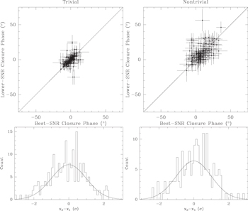
Figure 1. Consistency checks. Top: multiple processings of the same trivial (left) and nontrivial (right) closure phases are consistent with much less than the thermal noise. Bottom: pairwise differences of similar data points (as defined in Section 3.2) are consistent with being drawn from a Gaussian random distribution characterized by their error bars, confirming that the error estimates are not biased.
Download figure:
Standard image High-resolution imageThere are two classes of triangles on which we obtain closure phases. Triangles that include two VLBI stations from the same site (e.g., DFS) should produce closure phases that are trivially zero to within measurement error. On the intrasite baseline of these “trivial” triangles, the large-scale emission in the Galactic Center (on scales  ) is resolved out. Sgr A* is then pointlike, causing the intrinsic source phase to be zero. The two long baselines effectively sample the same (u, v) point, adding a source phase on one baseline and subtracting it on the other. There is no evidence of nonzero closure phases on Sgr A* or other sources in our data on the trivial triangles. “Nontrivial” closure phases on triangles involve one CARMA station, one station in Hawaii, and the SMT; these may be nonzero due to source structure.
As another consistency check, we examined measurements of closure phases that should be identical to within their errors. It is possible that variations in Sgr A* may cause fluctuations in the closure phase from scan to scan. However, during any particular scan, it is possible to obtain more than one estimate of trivial and nontrivial closure phases due to duplications among the stations. The closure phases obtained in the low and high bands should be identical, because the fractional frequency difference between the observing bands is very small. Closure phases on, for example, the FPS (LCP) and GJT (RCP) triangles should be identical, because Sgr A* exhibits almost no circular polarization at these frequencies (Muñoz et al. 2012; Johnson et al. 2015). Similarly, simultaneous closure phases on pairs of triangles that share the same sites but with different stations (e.g., DPS and FPS) should provide measurements of the same value. As expected, the pairwise differences of substantially identical closure phases are consistent with a unit Gaussian distribution centered on zero when the differences are normalized by the quadrature sum of the errors of the closure phases (bottom panels of Figure 1). This also provides evidence that the closure phase error bars are correctly estimated.
4. RESULTS
In total we detect 181 unique nontrivial closure phases for Sgr A* on the California–Hawaii–Arizona triangle. We additionally detect 233 trivial closure phases. Detected scan-averaged closure phases are listed in Table 2.
Table 2. Detected Closure Phases
| Day of | UT Time | Closure | Bispectral | u12 | v12 | u23 | v23 | u31 | v31 | |||
|---|---|---|---|---|---|---|---|---|---|---|---|---|
| Year | Year | (hr) | Banda | Triangleb | Phase ( ) ) |
S/N | (Mλ) | (Mλ) | (Mλ) | (Mλ) | (Mλ) | (Mλ) |
| 2009 | 93 | 11.5417 | H | CJS | −21.4 | 3.78 | −2548.3 | −1691.2 | 3044.2 | 1591.4 | −495.8 | 99.8 |
| 2009 | 93 | 11.9583 | L | CJS | 17.1 | 4.37 | −2658.9 | −1553.0 | 3191.9 | 1425.8 | −533.0 | 127.2 |
| 2009 | 93 | 11.9583 | L | DJS | 13.3 | 4.57 | −2658.9 | −1553.0 | 3191.9 | 1425.8 | −533.0 | 127.1 |
| 2009 | 93 | 12.2917 | L | DJS | −14.0 | 4.09 | −2724.4 | −1438.7 | 3282.6 | 1288.4 | −558.2 | 150.3 |
| 2009 | 93 | 12.6250 | L | CJS | −11.1 | 4.25 | −2769.2 | −1322.1 | 3348.2 | 1147.6 | −579.1 | 174.5 |
| 2009 | 93 | 13.1250 | H | CJS | 9.6 | 8.74 | −2796.5 | −1144.7 | 3398.5 | 932.6 | −602.0 | 212.1 |
| 2009 | 93 | 13.4583 | H | CJS | 4.3 | 7.03 | −2788.0 | −1026.1 | 3399.6 | 788.2 | −611.6 | 237.9 |
| 2009 | 93 | 13.4583 | L | CJS | −3.0 | 7.30 | −2788.0 | −1026.1 | 3399.6 | 788.2 | −611.6 | 237.9 |
| 2009 | 93 | 13.8750 | H | CJS | 18.3 | 6.97 | −2747.3 | −879.2 | 3364.4 | 608.7 | −617.0 | 270.5 |
| 2009 | 93 | 13.8750 | L | CJS | 33.7 | 8.53 | −2747.3 | −879.2 | 3364.4 | 608.7 | −617.0 | 270.5 |
Notes.
aHigh or Low band, as defined in Section 2. bStation codes are defined in Table 1.Only a portion of this table is shown here to demonstrate its form and content. A machine-readable version of the full table is available.
Download table as: DataTypeset image
The data are shown in Figure 2. There are more data points in later epochs due to the increased sensitivity provided by phased sma and, later, phased carma. Medians of the nontrivial closure phases are presented in Table 3, along with bootstrap estimates of the 95% confidence interval of the median, derived from random resampling with replacement.
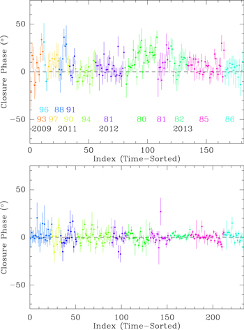
Figure 2. Top: all 181 nontrivial California–Hawaii–Arizona closure phases measured on Sgr A*. Data are presented in time order and are color-coded by day and year. The median nontrivial closure phase is  . Bottom: the 233 trivial closure phases for Sgr A*, excluding data from 2009 (Section 2.1.1). The median trivial closure phase is consistent with zero, as expected.
Download figure:
Standard image High-resolution imageTable 3. Median Closure Phases of Sgr A* on the California–Hawaii–Arizona Triangle
| 95% Rangea | |||||
|---|---|---|---|---|---|
| Year | Day(s) | N | Median | Low | High |
| 2009 | 093 | 11 | 9.6 | −11.1 | 17.7 |
| 2009 | 096 | 3 | 7.1 | ⋯ | ⋯ |
| 2009 | 097 | 10 | 8.4 | 0.7 | 13.5 |
| 2009 | All | 24 | 8.4 | 0.7 | 13.5 |
| 2011 | 088 | 7 | 13.6 | −0.4 | 29.0 |
| 2011 | 090 | 2 | 10.0 | ⋯ | ⋯ |
| 2011 | 091 | 5 | 5.7 | −5.9 | 11.7 |
| 2011 | 094 | 17 | −0.3 | −7.2 | 2.7 |
| 2011 | All | 31 | 2.6 | −3.5 | 5.7 |
| 2012 | 081 | 25 | 3.1 | −1.8 | 6.5 |
| 2013 | 080 | 28 | 16.0 | 6.7 | 20.2 |
| 2013 | 081 | 10 | 7.2 | −7.7 | 12.7 |
| 2013 | 082 | 15 | 10.3 | −0.5 | 14.1 |
| 2013 | 085 | 32 | 6.5 | 0.5 | 7.1 |
| 2013 | 086 | 16 | 3.0 | −1.6 | 6.3 |
| 2013 | All | 101 | 6.9 | 5.6 | 9.4 |
| All | All | 181 | 6.3 | 4.3 | 7.0 |
Notes. All closure phases are measured in degrees.
aThe 95% confidence interval of the median is estimated from bootstrap analyses using 107 resampled data sets.Download table as: ASCIITypeset image
The median closure phase (+63) on the California–Hawaii–Arizona triangle is positive at high statistical significance. In a larger run of 108 bootstrap-resampled data sets, every median was positive. This result is also robust against the exclusion of data from the day with the largest closure phase (2013 day 080); the resulting data set has a median closure phase of 5
0 with a 95% lower bound of 3
1. For comparison, the median trivial closure phase is 0
4, consistent with zero (95% range: −0
2 to
 ) as expected. The median nontrivial closure phase of +6
3 is too large to be attributable to instrumental effects (
7 measured in an independent analysis of 2013 data by R.-S. Lu et al. (2016, in preparation), using both the Mark 4 and DiFX correlators.
Care must be taken not to overinterpret differences between subsamples of the data set. When individual days of data are processed in multiple ways, the median closure phase can differ by a few degrees. This is particularly true for data taken in 2009 and 2011 (before the sensitivity of the observing array was increased) or for subsamples consisting of only a few measurements, where the inclusion or exclusion of one or two marginal detections can have a greater impact on the derived median value. For instance, the median closure phase on 2011 day 094 increases from −03 to
 when only self-calibrated data points are considered. The data set taken as a whole is large enough to be robust against the details of the processing to within a few tenths of a degree.
Because each baseline samples different (u, v) points at different times due to the Earth’s rotation, it would be possible for the closure phase to vary as a function of time, even if Sgr A* did not exhibit variability. Indeed, there is a trend for the measured California–Hawaii–Arizona closure phase to be larger later in the observing track (Figure 3). The  per degree of freedom for the best-fit line is 1.43, indicating that there is additional variability and/or that the increase with time is not linear. This increase with GST is significant at a level of
  using a Kendall tau test. The expected functional form as a function of GST is model-dependent, although the general trend for the California–Hawaii–Arizona closure phase to increase with time over an observing night provides an important constraint for physically motivated models of the 1.3 mm emission region in Sgr A*.
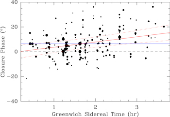
Figure 3. Measured closure phases (dot diameter proportional to S/N) plotted against GST. The solid red line shows the best-fit line, with the dashed red lines showing the  range. The solid blue line shows the best-fit line with zero slope. Despite the large scatter, the data suggest that the California–Hawaii–Arizona closure phase may be increasing with GST.
Download figure:
Standard image High-resolution image5. DISCUSSION
Our data clearly demonstrate that the closure phase on the California–Hawaii–Arizona triangle is nonzero, with a trend for the magnitude of the closure phase to increase over the course of a night. The sign and approximate value of the closure phase are consistent among multiple observing epochs over four years. In this section we consider the implications of these results.
5.1. Implications of Nonzero Closure Phase
The detection of nonzero closure phase is an unambiguous indication that these EHT data are resolving structure in the image of Sgr A*. Two robust conclusions are that the morphology of the emission from Sgr A* at 1.3 mm cannot exhibit point symmetry and that the millimeter emission is asymmetric on scales of a few Schwarzschild radii.
The sign of the closure phase resolves 180° rotational ambiguities in models. As an example, the best-fit parameters for the Broderick et al. (2011a) model find that the rotation axis of the accretion disk points toward either −52° or +128° ( error
error  ) east of north. This pair of directions was obtained from visibility amplitude information alone, which cannot discriminate between the two directions because the Fourier transforms of an image and the same image rotated 180° are identical modulo a sign flip in phase. Therefore, visibility phase or closure phase information is required to break the 180° degeneracy. The +128° direction is consistent in sign with our measured closure phases. Adding the new closure phase data is likely to result in better estimates of model parameters and to provide stronger constraints on models, including those that allow for deviations from general relativity (e.g., Broderick et al. 2014).
5.1.1. Accretion Models
The detection of nonzero but small closure phases in the image of Sgr A* demonstrates the power of imaging observations in placing strong constraints on its accretion flow geometry. In particular, the data favor emission morphologies that are connected rather than those composed of disjointed regions at horizon scales. At this point, it is instructive to look at the images generated in different general relativistic magnetohydrodynamic (GRMHD) simulations in order to explore in more detail how our observations can be used to constrain various configurations that are physically plausible and consistent with all other currently available data.
The parameters of GRMHD simulations are typically calibrated to reproduce the broadband spectrum of Sgr A* and the overall size of its emitting region at 1.3 mm. Even with these constraints imposed, however, the images they generate can be quite different from one another, depending on the prescription for the plasma thermodynamics that was employed, as well as on the initial magnetic field configuration and the tilt of the torus that was used to feed the black hole.
In a set of simulations referred to by Narayan et al. (2012) as Standard and Normal Evolution, the magnetic flux remains modest (e.g., De Villiers et al. 2003; Gammie et al. 2003). If the electron temperature is assumed to be at a constant ratio with the ion temperature everywhere in the flow, the generated images typically show continuous crescent-like brightness distributions (Dexter et al. 2009, 2010; Mościbrodzka et al. 2009, 2012; Chan et al. 2015). On the other hand, if the electrons in the jet are allowed to be heated much more strongly than within the disk, the images are characterized by bright regions from the inner walls of the jets, dissected by the cooler accretion disks (Mościbrodzka & Falcke 2013; Mościbrodzka et al. 2014; Chan et al. 2015). The relative brightness of the two regions (and their exact shape) depends on the inclination of the observer. Images with even more disjointed bright regions arise in Magnetically Arrested Disk simulations (MAD in the terminology of Narayan et al. 2012; see also McKinney & Blandford 2009 and Dexter et al. 2012 for similar magnetically dominated simulations and their applications to EHT observations of M87) and are dominated by emission from the footpoints of the jets (Chan et al. 2015). Finally, images with separated bright regions arise naturally in GRMHD simulations in which the accreting material is fed to the black hole from a plane that has a tilt with respect to the black hole spin (Dexter & Fragile 2013) because of the presence of standing shocks in these flows.
Comparing the detailed predictions of these simulations to our data is beyond the scope of this paper. However, motivated by the rather general properties of the disjointed geometries in the images exhibited by some of the GRMHD simulations, we discuss in the following how the observations reported here can be used to constrain such configurations.
5.1.2. Constraints on Disjoint Bright Regions
The gross characteristics of the jet-dominated images with disjointed bright regions (see Mościbrodzka & Falcke 2013; Mościbrodzka et al. 2014; Chan et al. 2015) can be captured by a simple geometric model composed of two separated regions that are symmetric and identical except for a difference in the brightness of each component. The closure phases of such a configuration will be equivalent to an even more reduced model in which the two regions are replaced with point sources. In this reduced model, the visibilities are analytically calculable as  , where r represents the amplitude ratio of the two components, and x and y refer to their separation east and north, respectively.28
Figure 4 shows the separations between two point sources that are consistent with our data. These separations would produce California–Hawaii–Arizona closure phases that are between  and
and  , the range of values implied by the best-fit line in Figure 3, at all GST times for which we have measured closure phases. Both r = 0 (one point source) and r = 1 (two equal point sources) are inconsistent with our data, because each would produce closure phases that are identically zero or 180°. For a separation comparable to the shadow diameter, the closure phase data imply that a disconnected two-component model would be oriented roughly east-west with the brighter component located to the west (Figure 4). If the emission from Sgr A* is coming from the footpoints of a MAD-type jet, this is inconsistent with the orientations of the Li et al. (2013) jet or Bartko et al. (2009) clockwise disk (see extended discussion in Psaltis et al. 2015a), but aligned with the preferred axis of the intrinsic emission at 7 mm (Bower et al. 2014). Closure phase measurements at 86 GHz already rule out asymmetric jet structures on larger angular scales from a few hundred microarcseconds to a few milliarcseconds (Park et al. 2015).
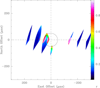
Figure 4. Offsets between two point sources that would produce closure phases between +09 and +14
9 at all triangles of (u,v) coordinates sampled by our data. For a unit point source centered at the origin, the colored regions indicate the allowed offset of a second point source, with color indicating the maximum value of r within the range
 . The circle shows an offset of 50 μas, which is approximately the diameter of the predicted shadow in Sgr A*. For two components separated by the shadow diameter, a roughly east-west alignment with the brighter component to the west is required to be consistent with our data.
Download figure:
Standard image High-resolution image5.2. Consistency of Closure Phases
5.2.1. Alignment of the Accretion Disk and Black Hole Spin Axes
The closure phase on the California–Hawaii–Arizona triangle is consistent in sign and magnitude, to within measurement error, from day to day. These observations span a four-year timescale that is much longer than the orbital period at the innermost stable circular orbit, which ranges from a few minutes to about half an hour, depending on the spin of the black hole. It is also larger than the Lense–Thirring precession timescale for a tilted accretion disk, unless the effective outer accretion flow radius is very large or the black hole spin is very small (Fragile et al. 2007; Dexter & Fragile 2013).
Misalignment of the spin axes of the accretion disk and black hole could produce two different observational consequences. First, it is possible that the inner disk could have a stable but slowly precessing structure. Examination of each epoch of the data in the context of disk (e.g., Broderick et al. 2009a, 2011a) or geometric crescent models (Kamruddin & Dexter 2013) may be able to place limits on the amount of precession.
Second, misalignment could result in multiple bright regions in the accretion flow due to standing shocks. GRMHD simulations of the accretion flow find that the separation between these regions is comparable to the diameter of the photon ring, although the emission pattern can be quite complicated in general (Dexter & Fragile 2013). Because the standing shocks can travel faster than the Lense–Thirring precession speed, the accretion flow would be expected to have a substantially different structure in different years, and very likely on different days within each year. The predicted closure phases over the course of a day on the California–Hawaii–Arizona triangle for the 515 h model of Dexter & Fragile (2013) mimic the rough range of closure phases observed, including a general trend of increasing value with GST. Further study is required to determine whether such a model predicts excess variability in closure phases and long baseline amplitudes beyond what is observed. The increased sensitivity of the EHT in upcoming years will be helpful for examining variability on intraday timescales.
5.2.2. Connections with the Accretion Rate
The discovery of the G2 gas cloud on an orbit with a close approach to Sgr A* (Gillessen et al. 2012) sparked interest in the possibility that the accretion rate of Sgr A* would increase due to the introduction of additional material into the accretion flow. Most of the material in G2 did not pass through pericenter until after the final epoch of observations reported herein (Gillessen et al. 2013), and mounting evidence suggests that G2 contains a star and is therefore not a pure gas cloud (Eckart et al. 2014; Witzel et al. 2014; Valencia-S. et al. 2015). In any case, the infall timescale is on the order of years (Burkert et al. 2012), so it would not be expected for there to be observational signatures of the G2 event in these data. However, there is evidence that G2 is a knot in a larger gas streamer that also includes the G1 gas cloud, which reached pericenter in the middle of 2001 (Pfuhl et al. 2015). If so, the accretion flow of Sgr A* could be supplemented with material from G1 or other gas in the streamer, with the caveat that some of the material deposited in the outer accretion flow may be carried away by outflows rather than making it to the inner region traced by the 1.3 mm emission (Wang et al. 2013).
The consistency of closure phases across multiple epochs from 2009 through 2013 provides evidence against large changes in the accretion rate over this period, which is consistent with the results of radio and millimeter-wavelength monitoring during the G2 encounter (Bower et al. 2015). The GRMHD simulations of Mościbrodzka et al. (2012) are instructive. When the accretion rate is decreased, the effective size of the accretion region decreases, with the result that the Hawaii–Arizona and Hawaii–California baselines do not adequately resolve the 1.3 mm emission region, causing the predicted closure phases to drop very close to zero. As the accretion rate is increased, the effective size of the emission region becomes larger, producing larger closure phases as the fringe spacing of the Hawaii–Arizona and Hawaii–California baselines becomes better matched to the asymmetric emission region. These larger closure phases persist even at the largest accretion rates modeled by Mościbrodzka et al. (2012), where the shadow of the emission region is obscured by the high optical depth of the accretion flow. This behavior is also seen when the accretion rate of the Broderick et al. (2011a) radiatively inefficient accretion flow models is varied. The average California–Hawaii–Arizona closure phase may therefore provide information complementary to visibility amplitudes in determining the overall accretion rate of the Sgr A* system.
5.2.3. Limits on Refractive Phase Noise
Scattering in the tenuous plasma of the interstellar medium affects the image of Sgr A* at radio wavelengths. The biggest effect of this scattering is to blur the image of Sgr A*, causing its apparent size to vary approximately as the square of the observing wavelength (Davies et al. 1976; Lo et al. 1981; Doeleman et al. 2001; Bower et al. 2006, and many others). A secondary effect of scattering is to introduce a variable substructure within the scattered image (Gwinn et al. 2014; Johnson & Gwinn 2015). Both of these effects can modify VLBI observables.
The formalism of Narayan & Goodman (1989) and Goodman & Narayan (1989) distinguishes between three different regimes of scattering. In the snapshot regime, diffractive scattering from small-scale inhomogeneities dominates. In the average regime, diffractive scattering is quenched, but refractive scintillation from large-scale inhomogeneities persists. In the ensemble-average regime, both diffractive and refractive scintillation are suppressed, and the scattering produces a deterministic blurring of the image. Due to the intrinsic size of Sgr A* as well as the integration time and bandwidth used in VLBI observations, the average regime is applicable to EHT observations of Sgr A* over the course of a single night. The ensemble of many nights of observations will tend statistically toward the ensemble-average regime, in which the observed visibilities are the intrinsic visibilities downweighted by a real Gaussian whose width in baseline space is inversely related to the size of the scattering ellipse. In the ensemble-average regime, the effects of scattering—blurring of the image—are invertible and do not affect closure phases (Fish et al. 2014).
However, in the average regime, image distortions and refractive substructure can introduce nonclosing phases. The magnitude of these effects may be up to 50 mJy in the visibility domain, with the peak effect at baselines near the length at which the ensemble-average visibility of a point source falls to  (Johnson & Gwinn 2015). This could be as large as a 10% effect on top of source visibilities of approximately 500 mJy on the baselines between Hawaii and the mainland United States (Fish et al. 2011), corresponding to a phase noise of ∼6°. However, this refractive phase noise will be partially correlated when the antennas are located within a few thousand kilometers of each other, so the net effect on closure phases on the California–Hawaii–Arizona triangle will be smaller.
Because refractive phase noise will fluctuate randomly about zero on timescales of about one day (Fish et al. 2014), it cannot account for the nonzero closure phases that we measure, which show a strong tendency to be positive. Nor can refractive phase noise account for the dependence of closure phase on GST. Thus, our measurements are a secure indication of intrinsic source asymmetry and do not merely reflect scattering-induced asymmetrical substructures. However, refractive variations may contribute to smaller interday variations in closure phase. Further observations at a range of wavelengths will be required to characterize the properties of the turbulent scattering screen and better understand its contribution to the apparent variability of Sgr A*.
6. CONCLUSIONS AND FUTURE PROSPECTS
We obtained 181 measurements of the closure phase at 1.3 mm on the California–Hawaii–Arizona triangle from 2009 to 2013. The median closure phase is nonzero at high statistical significance. This provides the first direct evidence that the structure of the 1.3 mm emission region is asymmetric on spatial scales comparable to the diameter of the shadow around the black hole that is predicted by general relativity. If the 1.3 mm emission arises from a MAD-like jet whose emission is concentrated in two disjointed bright regions separated by the shadow diameter, our data place a very strong constraint on its orientation. The data also provide important constraints for parameters of other outflow and accretion models of Sgr A*.
The constancy of the sign of the closure phase argues for the persistence of an asymmetric quiescent structure in Sgr A* likely coupled with some structural variability, consistent with simulations of a dynamic, spin-aligned accretion disk. While it is not currently possible to entirely disentangle the effects of variability in the structure of the emitting material around Sgr A* from the apparent substructure introduced by variations in the scattering screen, the California–Hawaii–Arizona closure phases indicate that refractive phase noise is not dominant on baselines between Hawaii and the western United States. These results are encouraging for producing an image of the quiescent emission by averaging several nights of data to mitigate intrinsic source variability and refractive substructure (Lu et al. 2015).
Closure phase measurements will soon provide much stronger constraints on source structure. In the near term, EHT observations in 2015 and beyond will incorporate additional observatories, including the Large Millimeter Telescope in Mexico, providing closure phase data on new triangles with higher angular resolution. Increasing data rates, starting with dual-polarization 2 GHz observations in 2015, will provide increased sensitivity that will result in larger detection rates and smaller random errors on each closure phase measurement, allowing interday and intraday variability to be tracked more accurately. Completion of the 1.3 mm VLBI array—including phased ALMA (Fish et al. 2016), the South Pole Telescope, the IRAM 30 m telescope at Pico Veleta, and the Northern Extended Millimeter Array at Plateau de Bure—will produce very sensitive data with good baseline coverage, culminating in the ability to reconstruct model-independent images of Sgr A*, M87, and other sources (Lu et al. 2014).
The EHT is supported by multiple grants from the National Science Foundation (NSF) and a grant from the Gordon & Betty Moore Foundation (GBMF-3561) to SSD. The SMA is a joint project between the Smithsonian Astrophysical Observatory and the Academia Sinica Institute of Astronomy and Astrophysics. The ARO is partially supported through the NSF University Radio Observatories program. The JCMT was operated by the Joint Astronomy Centre on behalf of the Science and Technology Facilities Council of the UK, the Netherlands Organisation for Scientific Research, and the National Research Council of Canada. Funding for ongoing CARMA development and operations was supported by the NSF and CARMA partner universities. A.E.B. receives financial support from the Perimeter Institute for Theoretical Physics and the Natural Sciences and Engineering Research Council of Canada through a Discovery Grant. Research at Perimeter Institute is supported by the Government of Canada through Industry Canada and by the Province of Ontario through the Ministry of Research and Innovation. M.H. acknowledges support from MEXT/JSPS KAKENHI. L.L. and G.N.O.L. acknowledge the financial support of DGAPA, UNAM, and CONACyT, Mexico. The EHT gratefully acknowledges equipment donations from Xilinx Inc.
Facility: EHT - .
APPENDIX: POTENTIAL SOURCES OF ERROR IN CLOSURE PHASE ESTIMATES
There are many places where potential errors may be introduced into VLBI data, including real-world imperfections in the signal chain and inaccuracies in the input model for correlation. Many potential sources of error close; among nonclosing errors, some introduce additional random (zero-mean) error into each closure phase estimate, while others may introduce biases. In order to characterize the significance of our results, we examine which errors might potentially bias closure phase measurements.
In this Appendix we consider potential sources of error from both theoretical and empirical perspectives. For the latter, we appeal to the data themselves to characterize potential biases. In addition to the Sgr A* data reported in this manuscript, two other sources from the 2013 observations provide high-S/N data to test whether potential sources of error introduce measurable biases into closure phase measurements. The source with the largest correlated flux density on long baselines in 2013 was BL Lac, for which a long series of consecutive scans on day 086 provides a large sample with high bispectral S/N on all triangles, often exceeding 100 on the FPS and GJT triangles. Another bright source that was observed over five nights in 2013, 3C 279, shows evidence of high polarization and complicated polarimetric structure on long baselines. We use data from these sources to estimate an upper limit of the magnitude of potential biases by considering matched pairs of simultaneously measured closure phases from two different data subsets (RCP versus LCP, high band versus low band, etc.) on both nontrivial and trivial triangles.
A.1. Clock and Position Errors
Each telescope uses a hydrogen maser as its timing and frequency standard. The maser signal is very stable over timescales of minutes, but usually exhibits a slow drift over longer timescales. The difference between a one pulse-per-second (PPS) signal from the maser and a PPS signal from the Global Positioning System (GPS) is logged over time, from which a time offset and drift rate are calculated. These parameters serve as inputs to the model used for correlation.
The correlator model also takes as inputs the locations of the telescopes and the celestial coordinates of the source. The location of each telescope, including the phase center of the phased arrays, has been measured with GPS. Errors on the order of centimeters to tens of centimeters may be possible due to a combination of GPS measurement errors and continental drift. Source coordinates are obtained from longer-wavelength VLBI catalogs and automatically corrected for precession. However, these coordinates may contain errors on the order of milliarcseconds, and in any case the centroid of emission at 1.3 mm may be different from that measured at a longer wavelength due both to frequency-dependent source structure and to intrinsic source variability.
Because of these effects, as well as a rapidly varying atmosphere, the a priori correlator parameters are close, though not perfectly correct, for modeling the delay and rate of a fringe. Fringe finding is required post-correlation in order to find residual delays and rates to compensate for errors in the model. However, the total quantities (delay and rate), the sum of the model, and residual quantities are independent of the input model, provided that the a priori model was within the effective correlator search windows (set by the accumulation period and spectral resolution). Thus, small station-based clock and position errors would not be expected to introduce biases into the closure phases calculated later in postprocessing.
A.2. Polarization Leakage
The receivers on the EHT telescopes were set up to receive left and right circularly polarized emission from the sky. Since no feed or polarizer (such as a quarter-wave plate) is perfect, a system set up to receive LCP will nevertheless detect a small portion of RCP emission, and vice versa.
The full equations for the correlated quantities, including polarization leakage, are
where numeric subscripts indicate antennas, letter subscripts indicate the sense of the circularly polarized feed, asterisks indicate complex conjugation, G indicates complex gain terms, D indicates polarization leakage terms, I and V indicate Stokes parameters representing the source total intensity and circular polarization,  indicates the combination of Stokes parameters representing the source linear polarization, and ϕ indicates the field rotation angle (Roberts et al. 1994). The field rotation angle depends on the mount of the telescope and the location of the receiver; for some EHT telescopes it is equal to the parallactic angle and for others it is the parallactic angle plus or minus the elevation angle.
Sgr A* exhibits very little (∼1%) circular polarization at 1.3 mm (Muñoz et al. 2012; Johnson et al. 2015), so circular polarization would not be expected to introduce an error of more than a few tenths of a degree in the closure phase from the terms without leakage (D) in Equation (1). As the field rotation angles rotate, the Stokes I terms vary as the difference of the field rotation angle between the two stations. In the absence of polarization leakage, the rotations introduced by the field rotation angles on three closing baselines cancel, producing no net change in the measured closure phase.
In contrast, Sgr A* exhibits high linear polarization at 1.3 mm. The median effective linear polarization fraction (P/I) ranges from about 5% on intrasite and SMT-CARMA baselines to 35% on the JCMT-CARMA baseline, with substantial additional variability (Johnson et al. 2015). Instrumental polarization leakage (D) terms for the EHT range from 1% at the SMA to 11% at the SMT, with a median value of about 5%. Polarization leakage can contaminate the RR and LL visibilities via the product DP, which for Sgr A* amounts to a few percent. This is not large enough for our measured median closure phase of  to be attributable to polarization leakage. Leakages vary as the sum of the field rotation angles of the stations on each baseline, with effects on RCP and LCP closure phases that are approximately symmetric but opposite in sign.
Assuming the median baseline-dependent polarization fractions and average polarization angles measured for Sgr A* in 2013 as well as the D-terms derived during instrumental polarization calibration, the typical biases expected to be introduced by polarization leakage are  over most of an observing track, with a maximum effect of about
  . The closure phase data on the most sensitive nontrivial LCP and RCP triangles (FPS and GJT, respectively) do not have sufficient S/N to be able to detect this difference. The trivial DFS and EGT closure phases are consistent with each other to less than
  , and the slope of their difference with time is consistent with zero. Neither BL Lac nor 3C 279 show a statistically significant bias between the LCP and RCP closure phases on any triangle (including the nontrivial California–Hawaii–Arizona triangle) or a slope with time.
A.3. Gain Errors
As can be seen in Equation (1), the complex gain (G) terms apply to the source term of each visibility as well as all of the leakage (D) terms. The closure phase is the argument of the product of three visibilities. Denoting gain-corrected source quantities (bracketed terms in Equation (1)) by ![$[\ldots ]$](https://content.cld.iop.org/journals/0004-637X/820/2/90/revision1/apj522974ieqn26.gif) , the measured closure phase is
, the measured closure phase is
Thus, station-based, frequency-independent complex gain errors do not introduce additional closure phase errors beyond those already present due to polarization leakage.
A.4. Bandpass Effects
Frequency-dependent bandpass errors can introduce closure phase errors. The bandpass response of a telescope is in general a complex quantity, containing both amplitude and phase structure.
HOPS provides partial mitigation of bandpass effects. The amplitude of each station is automatically normalized to the autocorrelation response on a per-channel level. This can theoretically still result in small errors when the autocorrelation response does not match the desired crosscorrelation response—for instance, if the IF response reduces sensitivity to sky signals near the edge of the band, or if subchannel structure in the bandpass response is significant.
EHT telescopes do not have a pulse calibration system to align the phases of each channel. Instead, the EHT data reduction uses manual instrumental phase calibration on very bright sources to derive phase offsets to apply to each channel on a per-station basis. The signal for all frequencies within each 480 MHz band passes through the same chain of electronics before being sampled by a single backend. As a result, the manual phases required to flatten the phase structure of the bandpass vary smoothly across the band. Before they are removed, channel-to-channel phase differences are typically a few degrees to  , with larger differences sometimes seen at the edges of the band.
Data from BL Lac indicate that any biases introduced by bandpass effects do not exceed a few tenths of a degree. High-band and low-band closure phases on nontrivial triangles agree to less than a degree. An additional test in which the low band was subdivided into two pieces (the first eight and the last seven channels) found consistent closure phases on all triangles at the level of  or better.
Footnotes
- 28
Since the closure phase is translation-invariant, we place one component at the origin for convenience.