Abstract
Chandra X-ray observations are analyzed for five galaxy clusters whose atmospheric cooling times, entropy parameters, and ratios of cooling time to freefall time within the central galaxies lie below 1 Gyr, below 30 keV cm2, and between 20 ≲ min(tcool/tff) ≲ 50, respectively. These thermodynamic properties are commonly associated with molecular clouds, bright Hα emission, and star formation in central galaxies. However, all have Hα luminosities below 1040 erg s−1 in the ACCEPT database. Star formation and molecular gas are absent at the levels seen in other central galaxies with similar atmospheric properties. Only RBS 0533 may host a radio/X-ray bubble, which are commonly observed in cooling atmospheres. Signatures of uplifted, high-metallicity atmospheric gas are absent. Their atmospheres are apparently thermodynamically stable despite the absence of strong nuclear feedback. We suggest that extended filaments of nebular emission and associate molecular clouds are absent at appreciable levels because their central radio sources have failed to lift low-entropy atmospheric gas to an altitude where the ratio of the cooling time to the freefall time falls below unity and the gas becomes thermally unstable.
1. Introduction
The central radiative cooling timescales of galaxy, group, and cluster atmospheres are often shorter than their ages. As the atmosphere cools and loses pressure support, it is expected to condense into molecular clouds at rates upward of 100 M⊙ yr−1 and to form stars. The atmosphere lost to cooling should be replenished by gas moving inward from larger radii in a slow, steady cooling flow (Fabian 1994). However, this phenomenon is not observed (Peterson & Fabian 2006).
Hot atmospheres are instead globally stable, in hydrostatic and thermal equilibrium. This stability must be maintained by one or more heat sources (Peterson & Fabian 2006; Pizzolato & Soker 2005, 2010), the most prevalent being mechanical feedback from a radio active galactic nucleus (AGN; Voit & Donahue 2005; McNamara & Nulsen 2007). Atmospheric density fluctuation spectra indicate that mild turbulence, presumably driven by rising X-ray bubbles, is able to gently heat atmospheres uniformly over the cooling regions (Zhuravleva et al. 2018). Thus, cooling flows do not form in stratified atmospheres, despite their relatively short central cooling timescales. Local atmospheric stability may prevail, in part, because their local dynamical timescales are shorter still than their cooling timescales at all altitudes.
Thermally unstable cooling is expected to occur when the ratio of the cooling timescale to the local freefall timescale falls near to and below unity (Nulsen 1986; Balbus & Soker 1989; Pizzolato & Soker 2005; McCourt et al. 2011; Voit & Donahue 2015; Prasad et al. 2018). This condition is never achieved, even at the very centers of clusters, where the cooling time falls below 1 Gyr. Instead, the ratio tcool/tff lies above 10 over the entire cooling region, including the center, where the cooling time is shortest (Hogan et al. 2017b; Babyk et al. 2019). This again indicates that atmospheres are largely thermally stable. Nevertheless, the filamentary nebular line emission and star formation observed in dozens of central galaxies (McDonald et al. 2016) indicate that atmospheres may be thermally unstable locally within a largely stable medium (McCourt et al. 2012).
Empirically, the hot atmospheres of central clusters and giant elliptical galaxies contain molecular clouds and young stars preferentially when the central atmospheric entropy and cooling timescales lie below K ≲ 30 keV cm2 and tcool ≲ 1.0 × 10⁹ yr, respectively (Cavagnolo et al. 2008; Rafferty et al. 2008). Such systems are much more likely to harbor the radio-inflated X-ray cavities that are stabilizing the atmosphere. Those with central cooling times exceeding 109 yr have a much lower incidence of radio emission (Main et al. 2017). These observations imply that gas supplied by cooling atmospheres is fueling the nuclear activity that is suppressing cooling and sustaining the feedback loop (Churazov et al. 2001; Pizzolato & Soker 2005; Gaspari et al. 2012). While the precise conditions under which thermally unstable cooling occurs in these systems are unclear, hot gas in the central regions of cooing atmospheres should eventually cool to low temperatures.
Pizzolato & Soker (2005) suggested that condensations of thermally unstable gas may form in the wakes of jets and radio lobes. Similarly, hydrodynamic simulations of jets advancing into hot atmospheres indicate that uplifted atmospheric gas and the ensuing turbulence may lead to preferential cooling in the wakes of rising X-ray bubbles (Revaz et al. 2008; Li & Bryan 2014; Brighenti et al. 2015; Voit et al. 2017; Gaspari et al. 2018).
ALMA and NOEMA observations of central galaxies have located molecular clouds preferentially in X-ray bubble wakes (Salomé et al. 2011; McNamara et al. 2014; Russell et al. 2017, 2019; Olivares et al. 2019), but it is unclear whether molecular clouds themselves are being lifted outward or whether the molecular clouds are condensing out of low-entropy hot gas lifted behind the bubbles (Salomé et al. 2008).
With the difficulty of lifting high column density clouds, McNamara et al. (2016) proposed that thermally unstable cooling is stimulated when a cooling, low-entropy, atmospheric gas parcel is lifted to an altitude where its freefall time exceeds its cooling time such that tcool/tff ≲ 1. Feedback then is thought to suppress cooling on large scales while simultaneously stimulating thermally unstable cooling in the vicinity of the bubble, ensuring a self-sustaining feedback loop. The loop may be stabilized, in part, by star formation, which would quickly consume the cooling gas, thus preventing it from overfeeding the black hole.
The ability to lift cooling gas in a galaxy may be key to triggering thermally unstable cooling. If so, cluster centrals with short atmospheric cooling times yet lacking cold clouds may also be devoid of X-ray cavities capable of lifting the low-entropy gas (McNamara et al. 2016). Here we further examine this hypothesis.
We have identified and analyzed five clusters drawn from the ACCEPT database (Cavagnolo et al. 2008) whose central atmospheric cooling times and central entropy parameters lie below 109 yr and 30 keV cm2, respectively. Furthermore, their central tcool/tff lie in the range of 10–30. Their atmospheric mean temperatures, within 100 kpc of the center, lie between 1.5 and 8 keV, and their central densities and pressures span more than a decade, in the range of 0.01–0.1 cm−3 and 10−10–10−9 erg cm−3, respectively. While small, the sample probes a broad range of environment, from groups to rich clusters.
Their atmospheric properties are similar to other cluster and group atmospheres rich in star formation and molecular gas. Yet these clusters are devoid of molecular gas and star formation at levels detected in other systems (McDonald et al. 2010, 2011). The analysis presented here shows that they are also devoid of X-ray bubbles capable of lifting atmospheric gas to an altitude where it is likely to become thermally unstable. This condition may explain, as we consider here, why these systems exhibit no spatially extended nebular emission like that seen in Perseus and other clusters. However, it begs the question of why they are apparently thermodynamically stable, when a distributed heat source is required to enforce this stability (McCourt et al. 2012). Either their atmospheres are being heated without the production of radio bubbles, or they are in a short-lived state.
Despite the absence of X-ray cavities in four of the five systems, their central galaxies have detectable radio emission, with A2029's being quite powerful. It is possible that atmospheric “sloshing” (Markevitch & Vikhlinin 2007) and/or the radio jets coursing through their atmospheres create mild turbulence capable of heating their atmospheres and temporarily balancing cooling in these systems (Gaspari et al. 2018; Voit 2018; Zhuravleva et al. 2018). While speculative, it serves to emphasize the interesting predicament these systems represent. We refer to them as “spoiler” clusters because they fail to exhibit the usual tracers of cold molecular clouds in their central galaxies that most other systems with similar atmospheric properties display.
Throughout this paper we assume a standard ΛCDM cosmology with H0 = 70 km s−1 Mpc−1, Ωm = 0.3, and ΩΛ = 0.7. All errors are 1σ unless otherwise stated.
2. X-Ray Data Analysis
Chandra X-ray data were obtained for A2151 and RBS 0540 and combined with preexisting observations from the Chandra Data Archive (CDA). The data for the remaining objects (A2029, RBS 0533, A2107) were obtained from the CDA. Cluster coordinates and details of X-ray observations are shown in Table 1. Each observation was reprocessed using the chandra_repro script with CIAO version 4.7. Bad grades were filtered out, and background light curves were extracted from level 2 event files. Events with time intervals affected by flares were eliminated using the lc_clean12 script.
Table 1. Chandra Data Used in Our Analysis
| Cluster | z | NH | ObsIDs | Total Exposure (ks) | Cluster Center | ||
|---|---|---|---|---|---|---|---|
| (1022 cm−2) | Raw | Cleaned | R.A. (J2000) | Decl. (J2000) | |||
| (1) | (2) | (3) | (4) | (5) | (6) | (7) | |
| A2029 | 0.0773 | 0.033 | 891, 4977, 6101 | 107.6 | 103.3 | 15:10:56.077 | +05:44:41.05 |
| A2107 | 0.0411 | 0.0445 | 4960 | 35.57 | 34.8 | 15:39:39.043 | +21:46:58.55 |
| A2151 | 0.0366 | 0.0334 | 4996, 19592*, 20086*, 20087* | 102.8 | 80.2 | 16:04:35.758 | +17:43:18.54 |
| RBS 0533 | 0.0123 | 0.102 | 3186, 3187, 5800, 5801 | 108.6 | 107.9 | 4:19:38.105 | +2:24:35.54 |
| RBS 0540 | 0.0397 | 0.0786 | 4183, 19593*, 20862*, 20863* | 64.5 | 61.6 | 4:25:51.300 | −8:33:38.00 |
Note. Column (1): redshift. Column (2): column density. Column (3): observation IDs used for the analysis. Column (4): raw combined exposure of the ObsIDs used. Column (5): usable exposure after data filtering. Column (6): R.A. Column (7): decl. Here, the asterisk denotes the new data obtained for A2151 and RBS 0540.
Download table as: ASCIITypeset image
Blank-sky backgrounds for each observation were extracted using CALDB version 4.6.7. Level 2 events files (and blank-sky backgrounds) were reprojected to match the position of the observation ID (ObsID) with the longest exposure time. Images were constructed in the energy range of 0.5–7.0 keV, for each ObsID. Point sources were identified using wavdetect (Freeman et al. 2002), visually inspected, and removed using CIAO. Spectra were extracted from concentric circular annuli centered on the cluster’s centroid. The innermost annulus was required to have a radius ≲10 kpc and binned to have a minimum of ∼3000 projected counts, with the number of counts per annulus increasing within each radial bin. Spectra were extracted from these annuli separately for each ObsID and were grouped with a minimum of 30 counts per energy bin.
Individually weighted redistribution matrix files and weighted auxiliary response files were created for each spectrum using mkacisrmf and mkwarf, respectively. Exposure maps were created for each ObsID and used to correct for the area lost to chip gaps, point sources, and vignetting. Lastly, spectra were deprojected using the geometric routine dsdeproj (Sanders & Fabian 2007; Russell et al. 2008).
3. Results
3.1. Image Analysis
Evidence for disturbances in the atmospheres that could be signatures of a bubble or cavity were investigated. Surface brightness profiles of the clusters were extracted from X-ray images, for a series of concentric annuli centered on the brightest pixel. After background subtraction, the resulting surface brightness profile may be fit with an isothermal β-model (Cavaliere & Fusco-Femiano 1976; Branduardi-Raymont et al. 1981):

where I0 is the central surface brightness, Rc is the core radius of gas distribution, and β is the slope. The single β-model is a poor fit to the surface brightness profiles. We instead fit the surface brightness profile with a double β-model, where the best-fitting double β-model was subtracted from the X-ray images in Figure 1. This difference is then divided by the best-fitting model to produce the residual images shown in Figure 2. This procedure accentuates fluctuations in the surface brightness of the intracluster medium (ICM) revealing substructure. The residual image also reveals structure to the north of RBS 0533 that may be a cavity or bubble. In Section 4.1, we estimate the significance of this region and draw conclusions on whether or not this structure is a bubble. The remaining clusters show evidence of variations in surface brightness, although none of these are likely due to bubbles or AGN feedback.
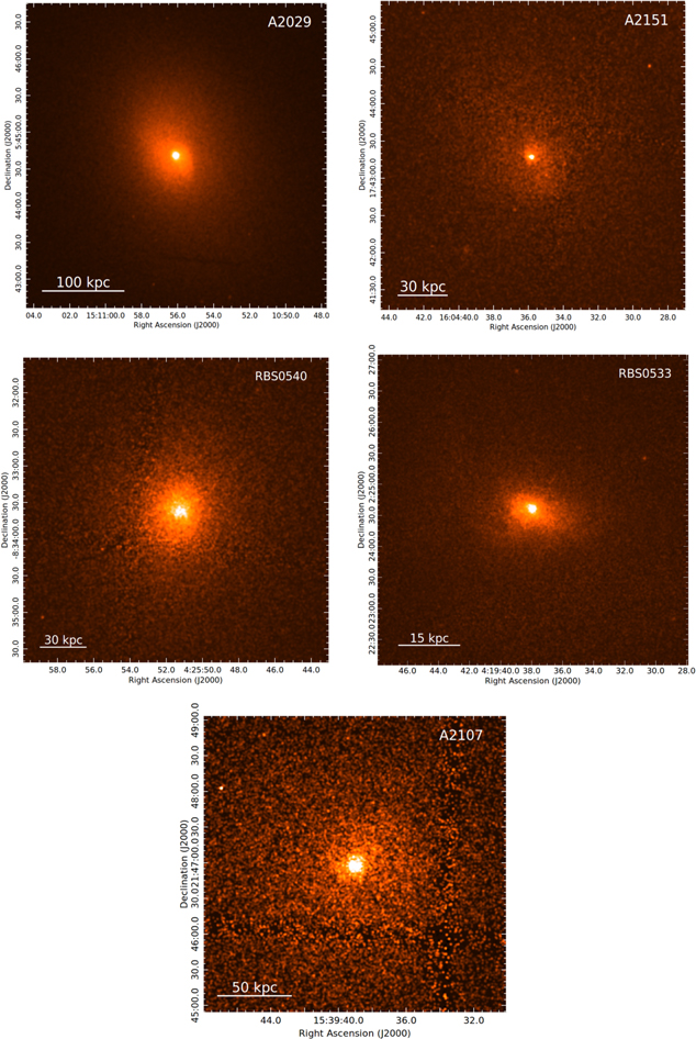
Figure 1. Background-subtracted and exposure-corrected images of the spoiler clusters; each image is Gaussian smoothed with a 3″ kernel radius. A clearly visible negative linear feature can be seen in A2029, which is due to the absorption by a foreground spiral galaxy (Clarke et al. 2004).
Download figure:
Standard image High-resolution image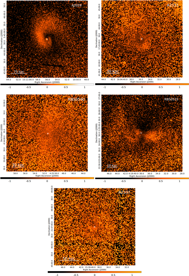
Figure 2. Model-subtracted relative residual images of each cluster. Images were obtained by fitting a double β-model to the cluster’s surface brightness profile of the form in Equation (1) and then taking the relative difference between the images in Figure 1 and that of the model. The white cross represents the location of the brightest pixel and is the center used in β-model fitting. These images are Gaussian smoothed with a 3″ kernel radius.
Download figure:
Standard image High-resolution imageFor instance, sloshing of intracluster gas can create sharp changes in temperature and density that appear as surface brightness edges when projected onto the sky (Markevitch & Vikhlinin 2007). These cold fronts are created by merging halos that displace low-entropy gas from the center of the potential that wraps into a spiral feature owing to sloshing motions. Such spiral features have been observed in many clusters, such as Perseus (Fabian et al. 2006), Virgo (Roediger et al. 2011), Centaurus (Sanders et al. 2016), A496 (Roediger et al. 2012), and A2029 (Paterno-Mahler et al. 2013).
Roediger et al. (2012) performed hydrodynamic simulations to explore the nature and origin of sloshing spiral features in A496. Cold fronts created in this simulation combined to form the observed spiral features, which are not necessarily a result of recent mergers. Ascasibar & Markevitch (2006) have shown that such features can persist for several gigayears. We explored our clusters for evidence of such features in the ICM.
In A2029, a cold front is clearly visible as a sharp change in surface brightness as seen in the top left image of Figure 1. Our residual image of A2029, shown in Figure 2, confirms the continuous spiral feature directly associated with the cold front. Its spiral feature is the largest and most continuous one known, extending outward radially from the center up to approximately 400 kpc (Paterno-Mahler et al. 2013).
Similarly, A2151's residual image also reveals a possible spiral feature. While not as prominent as A2029's sloshing feature, it extends radially outward to at least 81 kpc. We find no clear evidence of sloshing in the remaining objects.
3.2. Projected Thermodynamic Profiles
Spectra for each annular region were obtained using the method described in Section 2. Spectra were fit with the absorbed thermal model, phabs(apec). Abundances were determined relative to the values of Anders & Grevesse (1989). Excluding the redshift (frozen to the value of the cluster), all parameters—the column density of neutral hydrogen (NH), temperature, metallicity, and normalization—were allowed to vary. These values were used to derive the projected electron densities (ne),

where z is the redshift, N is the model normalization, DA is the angular diameter distance to the source, and V is the volume of a spherical shell with the inner and outer radii set to the annulus edges. The 1.2 factor is the ratio of the electron density to the hydrogen number density, ne/nH (Anders & Grevesse 1989). The cooling time of the ICM was calculated as

where p is the pressure, p = 1.8nekT, LX is the X-ray luminosity within each shell, and Λ(Z, T) is the gas cooling function in terms of abundance and temperature. LX was determined by first refitting spectra with a phabs × cflux(apec) model. We obtained an estimate for the X-ray bolometric flux by integrating the unabsorbed thermal model between 0.1 and 100 keV. The resulting X-ray flux was then converted to a bolometric X-ray luminosity, LX.
Finally, we derived the entropy parameter,  , and hot gas mass within each spherical shell, M = 1.9 μmpneV, where mp is the proton mass and μ = 0.62 represents the mean molecular weight of atmospheric plasma. Projected profiles are shown in Figure 3. Of these, A2029 spans a substantially larger temperature (3.0–9.5 keV) than the other clusters. Its density is nearly an order of magnitude higher than the other clusters; however, it still satisfies the threshold for central cooling time in projection.
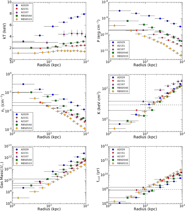
Figure 3. Projected temperature, pressure, density, entropy, gas mass, and cooling time profiles. The dashed horizontal lines represent the thresholds for the cooling time (tcool = 1.0 × 10⁹ yr) and entropy (K = 30 keV cm2). All errors here are reported at the 2σ level.
Download figure:
Standard image High-resolution image3.3. Deprojected Thermodynamic Profiles
Spectra extracted from the inner regions are affected by projected emission from the hotter regions of the atmosphere at higher altitudes. Accurately deriving the profiles of the inner regions of a cluster requires deprojection. This was done using the dsdeproj routine (Russell et al. 2008). Similar to our projected profiles, we fit the deprojected spectra to a single-temperature phabs(apec) model. Again, all parameters except for redshift were allowed to vary. Fitted quantities for temperature, abundance, and model normalization were used to derive the deprojected density, cooling time, entropy, and the hot gas mass profile, as shown in Figure 4. The deprojected profiles indicate that within the central region of each source (≲10 kpc), both the cooling time and the entropy lie below 1 Gyr and 30 keV cm2, respectively.
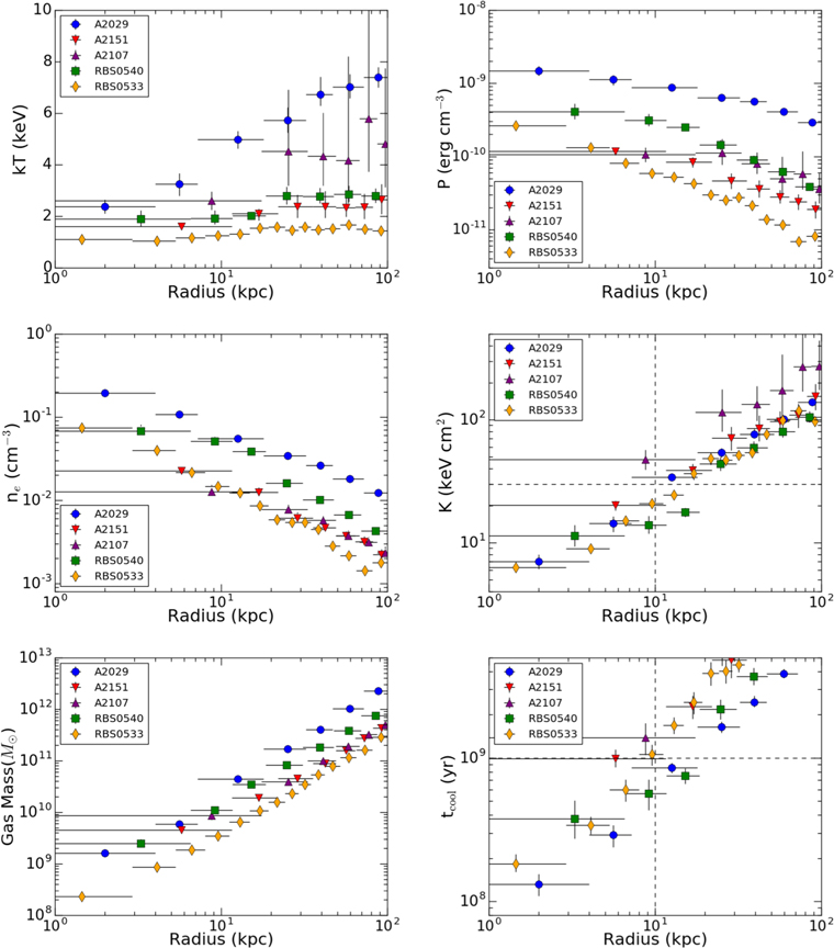
Figure 4. Deprojected temperature, pressure, density, entropy, gas mass, and cooling time profiles. The dashed horizontal lines represent the thresholds for the cooling time (tcool = 1.0 × 10⁹ yr) and entropy (K = 30 keV cm2). All errors here are reported at the 2σ level.
Download figure:
Standard image High-resolution imageThese objects span a moderate range of temperatures between 1 and 8 keV, while their radial densities and pressures span at least 2 orders of magnitude in the range of 10−1–10−3 cm−3 and 10−9–10−11 erg cm−3, respectively.
3.4. Mass Profiles
Mass profiles were created following the model presented in Hogan et al. (2017a). The model consists of a Navarro–Frenk–White (NFW) potential and a cored isothermal potential. The former has been shown to be an accurate description of the total gravitating potential of cluster masses on large scales (e.g., Pointecouteau et al. 2005; Vikhlinin et al. 2006) and takes the form of

where ρ is the characteristic gas density and Rs is the scale radius. Although the NFW profile provides a reasonable fit on large scales, its contribution alone underestimates masses inferred from stellar velocity dispersion due to the central galaxy (e.g., Fisher et al. 1995; Lauer et al. 2014; Hogan et al. 2017a). Thus, a cored isothermal potential is needed to account for this, given by

Here σ* is the stellar velocity dispersion and RI, which is used solely to prevent the gravitational acceleration from diverging from R → 0, is chosen to be smaller than the scales of interest. The combined NFW and cored isothermal potential, isonfwmass, is implemented as an xspec extension in the package clmass (Nulsen et al. 2010). The model assumes that the cluster atmosphere is spherically symmetric and in hydrostatic equilibrium.
Stable fits were found by following the work of Hogan et al. (2017a). The σ* parameter was frozen to the inferred stellar velocity dispersions derived from the Two Micron All Sky Survey (2MASS) isophotal K-band magnitude. When unavailable, values were taken from the HyperLEDA database (Makarov et al. 2014), or assumed to be 250 km s−1 when no data were available (Voit & Donahue 2015).
To compute the uncertainties in these quantities, xspec was used to create a Markov Chain Monte Carlo simulation of 5000 iterations. We adopted the 1σ standard deviation as the uncertainties in our mass profiles, as well as the uncertainties of Rs and  . The total cluster mass can then be computed at R2500, the radius where the mean density is 2500 times that of the critical density, ρc,

where  . The best-fitting parameters are shown in Table 2. The ratio of cooling time to freefall time is believed to be related to thermally unstable cooling (Nulsen 1986; Pizzolato & Soker 2005; McCourt et al. 2012), as such freefall time profiles are derived for each cluster. The enclosed mass profiles obtained from fitting are used to calculate the local gravitational acceleration, g = GM/R2, which can be used to calculate tff:

Table 2. Mass Fitting Parameters
| Cluster | σ* | AISO | Rs | ANFW | R2500 | M2500 |
|---|---|---|---|---|---|---|
| (km s−1) | (keV) | (arcmin) | (keV) | (kpc) | (1014 M⊙) | |
| (1) | (2) | (3) | (4) | (5) | (6) | |
| A2029 | 336 ± 10a | 0.694 |

|

|
693.4 |

|
| A2151 | 219 ± 4a | 0.295 |

|

|
259.2 |

|
| A2107 | 314 ± 25b | 0.608 |

|

|
414.6 |

|
| RBS 0533 | 306 ± 14b | 0.575 |

|

|
228.3 |

|
| RBS 0540 | 250 ± 15c | 0.384 |

|

|
279.5 |

|
Notes. Column (1): equivalent stellar velocity dispersion. Column (2): isothermal potential given by  . Column (3): NFW scale radius. Column (4): NFW potential given by
  . Column (5): R2500. Column (6): M2500.
Download table as: ASCIITypeset image
The enclosed cluster mass and freefall time profiles are shown in the top left and top right panels of Figure 5, respectively. The latter was used to create tcool/tff profiles shown in the bottom panel. The minimum tcool/tff values lie between 20 and 50, with A2029 residing at the lower end of this range and A2107 being at the higher end. Our min(tcool/tff) profiles differ from previous results but agree within a 1σ error for values calculated for A2029 (McNamara et al. 2016; Hogan et al. 2017a), A2151 (Pulido et al. 2018), and A2107 (Hogan et al. 2017a). These differences are likely due to contrasts in the size and number of spatial bins used for spectral extraction.
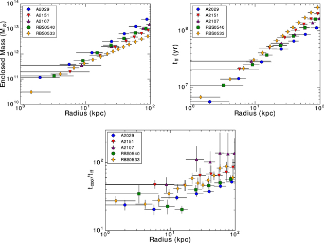
Figure 5. Top left: enclosed mass found from mass fitting; see Table 2. Top right: freefall profiles calculated using Equation (7). Bottom: deprojected tcool/tff profiles.
Download figure:
Standard image High-resolution image4. Quantitative Analysis
Visual inspection of images such as Figures 1 and 2 reveals two instances of sloshing swirls, in A2029 and A2151. The atmospheres of A2107 and RBS 0540 are nearly structureless. Only RBS 0533 has indications of surface brightness depressions consistent with an X-ray cavity or bubble. In this section, we present a method for estimating the significance of surface brightness depressions that can be used to determine whether or not these regions are X-ray cavities.
4.1. Surface Brightness Variations in the ICM
X-ray cavities are typically identified by surface brightness deficits of about 20%–30% relative to the surrounding medium (McNamara & Nulsen 2007, 2012). Panagoulia et al. (2014) showed that ∼20,000 counts within 20 kpc of the core are often required to clearly detect a cavity. Only A2029, RBS 0533, and RBS 0540 satisfy this criterion. Calzadilla et al. (2019) studied the surface brightness fluctuations in A1664 to determine whether two depressions surrounding the BCG are cavities or due to noise. Through significance tests, they determined that the regions were significant fluctuations and thus cavities.
We approached our analysis of surface brightness fluctuations by comparing the counts in the images of Figure 1, NI, to the counts in the best-fitting β-model image, NM. The model represents the undisturbed cluster atmosphere. We used the residual images in Figure 2 as a reference point for the location of potential bubbles in the ICM. We put circular regions of radius r over these depressions at distance R from the center and calculate the signal-to-noise ratio (S/N) in these regions to determine their significance. The signal within each generated region is calculated as

and the S/N within a region is estimated by

We calculate NM by fitting a double β-model and single β-model to the surface brightness profiles with both elliptical and circular annuli centered on the brightest pixel. The residual images reveal one cluster, RBS 0533, that possesses bubble-like structure to the north of its center. Since this bubble has no rims, making size estimates difficult, the size of the bubble was determined by calculating the S/N where the structure fades into the background (S/N < 5). This was done by overlaying box regions with fixed length and width, corresponding to 5.7 and 1.7 kpc, respectively. Regions are placed in succession of one another moving radially outward, beginning at roughly 2.5 kpc, where the depression is visible (see Figure 6). We find that at approximately R = 20 kpc (the edge of the yellow rectangle) the S/N falls below 5. Since the shape of the bubble is also unknown, we estimate the bubble as being spherically symmetric, which encloses the boxed regions (magenta circle).
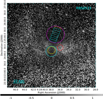
Figure 6. Model-subtracted relative residual image of RBS 0533 (same as in Figure 2) given by (NI − NM)/NM. Overlaid are circular regions used in significance testing (see Table 3), where the magenta circle is the approximate location and size of an X-ray bubble. Since the bubble has no clear rims, rectangular regions are used to find the approximate edge of a bubble where its structure is barely detected (S/N < 5), which corresponds to the yellow rectangle; see text for more details. Color regions to the south of the magenta circle may also be a cavity, although the S/N within these regions is low. This image is Gaussian smoothed with a 3″ kernel radius.
Download figure:
Standard image High-resolution imageThe S/Ns for the deficit in this circular region and for the other circular regions of interest are marked in Figure 6. The best-fit single and double β-models for elliptical and circular annuli are used to determine the deficits in these regions, and the S/N is calculated within each region using Equation (9). The details of this are given in Table 3.
Table 3. Signal-to-noise Ratio for Regions in RBS 0533 Fit with an Elliptical β-model and Circular β-model
| Elliptical Model | Circular Model | |||||||||
|---|---|---|---|---|---|---|---|---|---|---|
| Region Color | R | r | Single β-model | Double β-model | Single β-model | Double β-model | ||||
| (kpc) | (kpc) | Deficit (%) | S/N | Deficit (%) | S/N | Deficit (%) | S/N | Deficit (%) | S/N | |
| (1) | (2) | (3) | (4) | (5) | (4) | (5) | (4) | (5) | (4) | (5) |
| Magenta | 10.1 | 7.5 | −29.4 | 26.0 | −31.0 | 27.6 | −28.5 | 25.1 | −30.0 | 26.6 |
| Yellow | 4.5 | 3.2 | +2.5 | 1.6 | −2.4 | 1.6 | +5.1 | 3.1 | −0.2 | 0.1 |
| Cyan | 5.6 | 4.6 | +3.9 | 3.1 | −0.4 | 0.31 | +6.4 | 5.1 | +2.0 | 1.7 |
| Red | 8.6 | 2.5 | +47.3 | 14.8 | +39.2 | 12.8 | +54.6 | 16.4 | +47.2 | 14.8 |
Note. Column (1): region color in Figure 6. Column (2): distance away from the cluster center. Column (3): size of the region. Column (4): deficit of image relative to model (NI/NM − 1). Column (5): S/N given by Equation (9).
Download table as: ASCIITypeset image
The surface brightness deficit of this candidate bubble reaches 31% with an S/N of ∼28. These values are consistent with both elliptical and circular β-models, indicating that the structure is resilient to model parameters. Thus, it is likely real and is roughly consistent with the emissivity expected for an evacuated cavity relative to its surroundings (McNamara & Nulsen 2007).
Colored regions to the south of the center (cyan and yellow circles) were found to be insignificant and correspond to an excess of roughly 6% at most for the single circular β-model and a deficit close to 2% relative to the double elliptical β-model. The S/N is relatively low for all models in these regions, which suggests that the structure we see within these regions is likely not real, or rather, it may be an artifact from the model.
The red circle to the west of the center is a region of excess, which reaches levels of about 39% and 47% relative to the model corresponding to S/Ns of 13 and 15 for an elliptical and circular double β-model, respectively. This indicates that this structure is likely a real feature.
Extending this analysis to the other clusters, we find that no other clusters have significant structure associated with feedback, although the sloshing feature in A2029 has an S/N > 20, making it a conclusive detection, whereas the sloshing feature in A2151 has an S/N ≲ 5, making its detection uncertain.
Finally, we can obtain an estimate for the total energy required to inflate the bubble in RBS 0533, which is given by its enthalpy,

where p is the pressure within the cavity assuming that the cavity is in pressure balance with its surroundings, V is the volume of the cavity, and γ is the ratio of specific heat capacities. Here, γ is 4/3 for a relativistic gas and 5/3 for a nonrelativistic monatomic gas. Throughout our analysis, we assume that cavities are filled by a relativistic ideal gas, so E = 4pV. The age of a cavity is best represented by the buoyancy timescale, tbuoy, which is given by (Bîrzan et al. 2004; Vantyghem et al. 2014)

where S is the bubble’s cross section, V is the volume of the bubble, g is the local gravitational acceleration, and C = 0.75 is the drag coefficient (Churazov et al. 2001). The gravitational acceleration is estimated as g = GM/R2, where M is the total enclosed mass found in Section 3.4. The buoyancy time of the bubble is ∼1.3 × 10⁷ yr, which can be used to estimate the jet power, or the mechanical power of the AGN that would be required to inflate a spherical bubble of this size, given by

For a bubble of size r = 7.5 kpc at distance R = 10 kpc, the jet power is (3.5 ± 0.2) × 1043 erg s−1.
4.2. Undetected Cavities
Among the factors that govern the detection of cavities, high central surface brightness favors their detection in cool cores. Bîrzan et al. (2012) used a simulation to define the properties of bubbles that remain undetected. They concluded that most bubbles are undetected when the angle between the bubble-to-core axis and line of sight is small, or when they lie at large distances from the core.
Apart from RBS 0533, cavities may exist in these systems but remain undetected. Several studies have investigated the statistical properties of cluster cavities that are drawn from the Chandra archive. One such survey found a cavity detection frequency of 41% for a sample size of 75 clusters (Bîrzan et al. 2012), while a sample of 133 systems biased toward cool core clusters found a detection rate of 52% (Shin et al. 2016).
In the brightest 55-cluster sample (B55), it was shown by Dunn & Fabian (2006) that 20 of these clusters require heating to offset cooling. At least 14 of the 20 clusters have clear bubbles, and only one of these does not harbor a central radio source.
Finally, Dunn & Fabian (2008) studied the 42 clusters from the B55 and brightest cluster samples with Chandra data. Of those, 23 have a central radio source. Defining cooling flow clusters as those with a significant central temperature drop and a short central cooling time, they found that 14 of the 42 clusters met these criteria and 6 of those harbor bubbles.
The distribution of radio powers for this sample is consistent with expectations for cool core clusters (Hogan et al. 2015). Although only one of the five objects in our sample has a significant surface brightness depression that may be an X-ray bubble, apart from A2107, four of five possess a central radio source shown in Figure 7. It is noteworthy that the central radio source in RBS 0533 does not coincide with the surface brightness depression associated with the putative X-ray bubble. While this does not exclude the possibility that it is a “ghost cavity” whose radio emission has faded (Bîrzan et al. 2004), it is not a resounding confirmation that the surface brightness depression is indeed a radio/X-ray bubble. Our thermal instability analysis below assumes, conservatively, that it is indeed a bubble capable of lifting low-entropy gas outward.
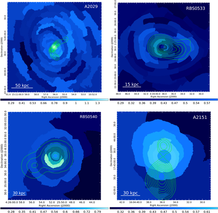
Figure 7. Metallicity maps of each cluster. Point sources were excluded from the images, where the color bar is given in units of Z⊙. The green contour lines are the radio data from the VLA FIRST survey shown at the 1.4 GHz frequency with a resolution of 5″. In A2029, the radio observation has an rms noise of 11.8 mJy, with contours starting from 5σ and increasing in steps of 0.001 × σ. In RBS 0533, the rms noise is 1.17 μJy, with the contours beginning at 8σ and increasing in steps of 0.5 × σ. RBS 0540's radio source has an rms noise at the 7.31 mJy level, with contours starting at 15σ and increasing in steps of 0.1 × σ. Lastly, A2151's radio source has an rms noise of 1.63 mJy, with contours starting at 3σ and increasing in steps of 0.2 × σ. These maps show no evidence of metal-enriched plasma lying preferentially along the jet axis.
Download figure:
Standard image High-resolution image4.3. Uplifted Metal-rich Atmospheric Gas
X-ray cavities not only displace hot gas but also may draw metal-enriched plasma out from the centers of clusters at rates of tens to hundreds of solar masses per year (Kirkpatrick et al. 2011; McNamara et al. 2014). The maximum radius that metals can be uplifted to, referred to as the iron radius, RFe, is correlated with Pjet according to the relation (Kirkpatrick & McNamara 2015)

Here Pjet is in units of 1044 erg s−1 and RFe is defined as the radial bin farthest from the cluster’s center where the 1σ error bars for the metallicity profiles (along the jet and orthogonal to it) do not overlap (Kirkpatrick et al. 2011). The scatter in the relation is large, approximately 0.87 dex. In clusters with known cavities, metal-enriched gas preferentially, but not exclusively, lies along the bubbles and thus the radio jets.
As a first step in a search for uplifted gas, we created metallicity maps using the contour binning algorithm of Sanders (2006). The metallicity maps are intended to provide a visual representation of the radial abundance distributions with respect to the radio sources. However, they are not used in our analytical evaluation of the relationship between the off-nuclear atmospheric gas abundance and the radio sources. Clusters were binned using a minimum S/N of 70 per bin to maximize the number of bins generated while retaining a high enough count per bin that uncertainties in metallicity do not dominate. No attempts were made to create maps for A2107, as its exposure time is too short, and thus its low number of counts would not allow us to generate enough bins with the required S/N for any meaningful analysis.
Spectra were extracted within each bin and fitted with a phabs(apec) model. Temperature, metallicity, and normalization were allowed to vary. Column densities were frozen at the value obtained from the LAB Survey (Kalberla et al. 2005). The resulting metallicity maps are shown in Figure 7.
Higher-metallicity gas aligned parallel and antiparallel to the jet axis is a strong indicator of metal-enriched gas being uplifted. The slightly asymmetric map near the center of RBS 0533 hints at this mechanism without being prominent enough to be deemed significant.
To further constrain the lack of evidence for uplifted metal-enriched gas in these four clusters, spectra were extracted from the profiles of annular sector bins with openings lying between 50° and 90°. One of these profiles is along where the extended radio emission from the jet is located (“along-jet”). Extracted spectra in these regions are assumed to reflect the impact of the AGN on the gas. Other profiles are extracted along a direction orthogonal to or offset from the jet axis (“off-jet”) and represent the undisturbed atmosphere. Spectra from these profiles are assumed to be representative of the average prior AGN outbursts. Extracted spectra were fit in the same manner as those used to make Figure 7. The results of this analysis are shown in Figure 8. A2029 demonstrates slight evidence of a trend in higher-metallicity gas along the jet axis, but only in bins between approximately 20 and 60 kpc outward from its center.
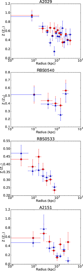
Figure 8. Metallicity profiles for the spoiler clusters, from top to bottom: A2029, RBS 0540, RBS 0533, A2151. Abundances along the jet axis are represented by red circles, while those for spectra in orthogonal directions or other off-jet locations are denoted by blue triangles. A2029's along-jet profile shown here is of its northwest jet. These profiles show no evidence that metal-enriched gas preferentially lies along the jet axis, which is consistent with Figure 7. All errors here are reported at the 2σ level.
Download figure:
Standard image High-resolution imageTo determine whether the along-jet and off-jet profiles differ significantly, and thus the likelihood that an abundance excess along the jet axis is significant, we perform two statistical tests for each of our clusters. The results of both statistical tests are shown in Table 4.
Table 4. Summary of t-tests and K-S Tests
| t-test | K-S Test | |||
|---|---|---|---|---|
| Cluster | p-value | Significant? | DK-S | Same Sample? |
| A2029 | 0.52 | No | 0.0506 | Same |
| RBS 0533 | 0.65 | No | 0.0191 | Same |
| RBS 0540 | 0.40 | No | 0.146 | Same |
| A2151 | 0.42 | No | 0.168 | Same |
Note. Results of our t-test and K-S test indicate no significant differences between along-jet and off-jet profiles in each of the clusters.
Download table as: ASCIITypeset image
In our first test we compare the means for two profiles, using them to calculate the likelihood that they are drawn from the same distribution using a two-tailed t-test. We choose to perform our tests at the 95% significance level (α = 0.05) with the null hypothesis that differences between mean profile metallicities are insignificant. In each of the clusters, the null hypothesis cannot be rejected at the chosen significance level.
Table 5. Cold Gas Measurements for the Spoiler Clusters: A Comparison of Hα Measurements from the ACCEPT Database versus Other Sources
| Corrected | ||||||
|---|---|---|---|---|---|---|
| Cluster | BCG | SFRUV | LACCEPT,Hα | LHα | SFRHα |

|
| (M⊙ yr−1) | (1040 erg s−1) | (1040 erg s−1) | (M⊙) | (108 M⊙) | ||
| (1) | (2) | (3) | (4) | (5) | (6) | (7) |
| A2029 | IC 1101 | <1.72 | <0.643 | <0.44 (1) | <0.035 | <17 (2) |
| A2151 | NGC 6041 | <0.38 | <0.141 | 0.032 (3) | 0.003 | <3.1 (2) |
| A2107 | UGC 09958 | <0.57 | <0.179 | ⋯ | ⋯ | ⋯ |
| RBS 0533 | NGC 1550 | <0.14 | <0.016 | ⋯ | ⋯ | <0.47 (4) |
| RBS 0540 | MCG-01-12-005 | 0.4 ± 0.09 | <0.011 | <0.014 (5) | <0.001 | ⋯ |
Note. Column (1): cluster. Column (2): BCG. Column (3): ultraviolet SFR from Hoffer et al. (2012). Column (4): ACCEPT database Hα luminosity (Cavagnolo et al. 2008). Column (5): Hα luminosity corrected for our chosen cosmology (see end of Section 1). Column (6): SFR from calculated Hα luminosity using SFRHα = 7.9 × 10−42 LHα (Kennicutt 1998). Column (7): molecular gas measurement from CO observations. References to LHα and  measurements: (1) McDonald et al. 2010; (2) Salomé & Combes 2003; (3) McDonald et al. 2011; (4) O’Sullivan et al. 2018; (5) Cavagnolo et al. 2009.
Download table as: ASCIITypeset image
In the second statistical test, a two-sample Kolmogorov–Smirnov (K-S) test is performed to determine whether both the along-jet and off-jet metallicity profiles are independent of one another, or come from the same distribution. Again, a significance level of α = 0.05 is chosen with a null hypothesis, that both distributions are drawn from the same parent sample. The null hypothesis is rejected at this significance level if the calculated K-S statistic, DK-S, satisfies the condition given by  , where n and m are the sizes of the along-jet and off-jet profiles, respectively. Similarly to the previous test, the null hypothesis cannot be rejected in any of the clusters.
At the 95% level, then, there is no significant difference between metallicity profiles in any clusters, and thus there is no evidence of uplifted metal-enriched gas. Indeed, extracting spectra along random directions not aligned with the jet axis generally yields profiles that show no evidence of trends in our sample. Subsequent statistical analysis of our profiles only further confirms the results.
5. Discussion
5.1. Thermally Unstable Cooling
Central galaxies located at the bases of hot atmospheres are often associated with molecular clouds, star formation, and nebular emission. Chandra observations have shown that they are prevalent when systems lie below the central cooling time and entropy thresholds (1 Gyr and 30 keV cm2, respectively), while those above are usually devoid of cool gas and star formation (Cavagnolo et al. 2008; Rafferty et al. 2008).
On a more fundamental level, hot atmospheres should be susceptible to thermally unstable cooling when the ratio, tcool/tff, falls below unity (Nulsen 1986; Pizzolato & Soker 2005; McCourt et al. 2012). In this context, the cooling time and entropy thresholds would be necessary but insufficient criteria. However, the local value of tcool/tff almost never lies below 10, even in systems experiencing vigorous star formation (Hogan et al. 2017b). Others have suggested that thermally unstable cooling occurs when this ratio lies well above unity, in the range of 10–30 (Gaspari et al. 2012; McCourt et al. 2012; Sharma et al. 2012).
Inspection of Figures 4 and 5 indicates that both the cooling time threshold and criterion are satisfied and that the min(tcool/tff) ∼ 20–50. The central galaxies in this sample should be thermally unstable and should be forming stars and shining by nebular emission. They are not. This failure to respond to both criteria calls for a third possible criterion, possibly uplift, which we have investigated in detail here.
We find surface brightness depressions consistent with an X-ray bubble only in RBS 0533. However, it lacks bright rims composed of low-entropy gas lifted from the inner region of the atmosphere. Furthermore, RBS 0533 and the remaining clusters show no other evidence of substantial uplifted atmospheric gas that would trigger thermally unstable cooling once the gas reaches an altitude where tcool/tff falls below unity. Therefore, the observations are consistent with the hypothesis that uplift may be a significant factor in driving thermally unstable cooling. This investigation does not constitute proof but may indicate that we are on the right track.
Another factor that may trigger thermally unstable cooling is mild atmospheric turbulence (Gaspari et al. 2018; Voit 2018). Turbulence may be induced by the peculiar motion of the central galaxy and mergers. However, in this context the driving mechanism would most likely be the central AGN. The absence of X-ray bubbles would imply the absence of a mechanism to drive the turbulence imparted on the lifted gas. The sloshing spiral in A2029 seen in Figure 2 is evidence of a merger and may indicate that it produced insufficient levels of turbulence required to trigger instabilities.
On the other hand, modest atmospheric turbulence may be a factor leading to the thermal stability of these systems through turbulent heating (Hitomi Collaboration et al. 2016; Zhuravleva et al. 2018). The situation is far from clear but will be further explored with the X-ray Imaging and Spectroscopy Mission and future X-ray observatories equipped with microcalorimeter spectrometers.
5.2. The Absence of Significant Cold Gas Mass
These objects were originally selected for observation on the basis of having upper limits on Hα luminosity as listed in the ACCEPT database (Cavagnolo et al. 2008). We have since performed an exhaustive literature search for more recent nebular and molecular mass measurements for each of the clusters. The results from this search are summarized in Table 5.
5.3. RBS 0533
ACCEPT lists an Hα luminosity for RBS 0533 as LHα < 0.016 × 1040 erg s−1. Two other studies that probed its central galaxy’s (NGC 1550) CO emission are in tension. O’Sullivan et al. (2018) detected no CO (2−1) or CO (1−0) emission, arriving at an upper limit for molecular hydrogen of MH2 < 0.47 × 10⁸ M⊙. However, Nakanishi et al. (2007) claimed a detection of CO (3−2) deriving a molecular gas mass of MH2 = 4.3 × 10⁸ M⊙. Clearly these measurements are inconsistent with each other. The apparent CO (3−2) line is broad, spanning a significant fraction of the receiver’s ∼445 km s−1 bandwidth, leaving little room for the baseline continuum to be evaluated. Taking all into account, we adopt the O’Sullivan et al. (2018) upper limit. RBS 0533's central cooling time and entropy both lie below their respective thresholds (109 yr and 30 keV cm2), and thus it is expected to shine in nebular emission.
We have shown in Section 4.1 that its atmosphere harbors a possible X-ray bubble. Therefore, the absence of spatially extended nebular emission is intriguing but not necessarily inconsistent with our hypothesis that thermally unstable cooling is stimulated by uplift. McNamara et al. (2016) suggested that bubbles must lift cool, atmospheric gas to an altitude where tcool/tff < 1. The cooling time of the atmospheric gas at the center of RBS 0533 is ∼108 yr. Based on Figure 5, this gas must be lifted to an altitude of nearly 40 kpc to meet this cooling criterion. However, the observed bubble, at least in projection, extends to roughly half this distance. Therefore, it is plausible that the bubble has not lifted enough atmospheric gas to stimulate thermally unstable cooling at an observable level.
5.4. A2151 and A2107
A2151's Hα luminosity is listed as LHα < 0.141 × 1040 erg s−1 in ACCEPT. McDonald et al. (2011) recently ejected Hα emission in its BCG, NGC 6041, with a luminosity of LHα ∼ 3 × 1038 erg s−1. Therefore, NGC 6041 has a detectable level, albeit a modest level of molecular gas. However, emission at this level lies well below the luminosity where the cooling time threshold seen in Cavagnolo et al. (2008) becomes prominent at, LHα ∼ 1040 erg s−1. An Hα detection of this magnitude is expected as the accumulation of gas from stellar winds, supernovae, and external accretion that may be unrelated to uplift and thermally unstable cooling. In A2107, we find no measurements for cold gas, and so the ACCEPT upper limit is adopted.
5.5. RBS 0540
RBS 0540's Hα luminosity, <0.014 × 1040 erg s−1 (Cavagnolo et al. 2009), agrees reasonably well with the value quoted in ACCEPT, <0.011 × 1040 erg s−1. This is also the only cluster in our sample with a detection for SFRUV of 0.4 ± 0.09 M⊙ yr−1 (Hoffer et al. 2012).
5.6. A2029
A2029's Hα luminosity is listed in the ACCEPT database as LHα < 0.643 × 1040 erg s−1. However, McDonald et al. (2010) found a more restrictive upper limit of <4.41 × 1039 erg s−1. This upper limit is surprising, as its central cooling time and bright, cuspy X-ray emission are similar to clusters with nebular emission luminosities exceeding this limit by more than three orders of magnitude. Why A2029's central galaxy lies dormant while others with similar or less extreme atmospheric properties burgeon with star formation has been a mystery for decades.
Further complicating the matter, A2029's central galaxy hosts a large and relatively powerful radio source P1.4 ∼ 1041 erg s−1. Therefore, it should in principle be able to lift hot gas outward, making it susceptible to thermally unstable cooling. However, no evidence for large cavities was found in A2029 by Paterno-Mahler et al. (2013) or in our analysis. A2029's radio source is long and thin (Figure 7). It lacks jets feeding high-volume lobes seen in other powerful sources such as Hydra A and MS 0735+096, which are lifting vast quantities of atmospheric gas (Kirkpatrick & McNamara 2015). It is unclear why this is so. It may be a consequence of atmospheric sloshing that may be sweeping the radio source back into a wide-angle tail morphology (Paterno-Mahler et al. 2013).
In the context of this discussion, the absence of prominent X-ray cavities or radio lobes may indicate that its radio source is incapable of lifting an appreciable amount of atmospheric gas. Its mechanical power may be too small despite its powerful synchrotron emission. Therefore, its atmosphere remains thermally stable, at least for the time being. It is unclear why this would be. Croston et al. (2018) have pointed out that Fanaroff and Riley (FR) type I and II radio galaxies have different particle contents, with FR I galaxies having higher jet (mechanical) power for their synchrotron luminosities than FR II galaxies. Perhaps A2029's radio source is composed of light particles akin to an FR II radio source rather than an FR I, which is commonly found at the centers of clusters.
6. Conclusions
In this paper we have studied five galaxy clusters using Chandra observations and archival data. The clusters were selected from the ACCEPT database on the basis of possessing an upper limit on nebular Hα emission. Our main findings are as follows:
- 1.Projected and deprojected thermodynamic profiles reveal that within the central 10 kpc of each cluster the atmospheric cooling time and entropy lie below 109 yr and 30 keV cm2, respectively. Below these thresholds, cool gas and star formation traced by nebular emission above ≃1041 erg s−1 are commonly observed (Figure 9).
- 2.Only RBS 0533 has atmospheric structure consistent with a possible X-ray cavity. The feature is a 31% depression in Figure 1 relative to the elliptical double β-model, with an S/N of ∼28.
- 3.While only one of five targets contains at least one cavity, four of the five clusters have radio emission as shown in Figure 7. This property is consistent with other systems with short central cooling times (Cavagnolo et al. 2008). The central galaxy in A2151 possesses weak Hα emission at the level of 3 × 1038 erg s−1. This level lies roughly 300 times below the level normally associated with cluster cooling. The absence of a significant levels of cold gas is consistent with the hypothesis that these objects are able to effectively lift low-entropy gas to an altitude where the atmosphere becomes thermally unstable, i.e., tcool/tff ≲ 1.
- 4.Thermodynamic profiles extracted along and off the jet axis show no evidence of uplift or that higher-metallicity gas lies preferentially along the jet axis. This is clearly evident in our abundance maps within Figures 7 and 8 and was confirmed more rigorously through statistical analyses using a t-test and K-S test.
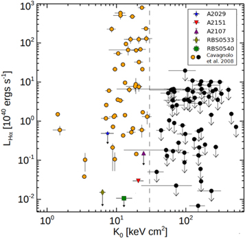
Figure 9. Central entropy (R < 10 kpc) plotted against Hα luminosity, adapted from Cavagnolo et al. (2008). Orange circles are Hα detections, and black circles are nondetections of the clusters plotted against the Hα luminosity. Overlaid are the points from our sample; all values are measured from Column (5) in Table 5, excluding RBS 0533 and RBS 0540, where the ACCEPT database values are plotted.
Download figure:
Standard image High-resolution imageWe thank Jeremy Sanders and Keith Arnaud for their support in troubleshooting software problems with contour binning and Xspec, respectively. M.T.H. and B.R.M. acknowledge funding from the Chandra X-ray Observatory Cycle 18 proposal for A2151 and RBS 0540. H.R.R. acknowledges support from an STFC Ernest Rutherford Fellowship and an Anne McLaren Fellowship.