Abstract
We analyze spatially resolved and co-added SDSS-IV MaNGA spectra with signal-to-noise ratio ∼100 from 2200 passive central galaxies (z ∼ 0.05) to understand how central galaxy assembly depends on stellar mass (M*) and halo mass (Mh). We control for systematic errors in Mh by employing a new group catalog from Tinker and the widely used Yang et al. catalog. At fixed M*, the strengths of several stellar absorption features vary systematically with Mh. Completely model-free, this is one of the first indications that the stellar populations of centrals with identical M* are affected by the properties of their host halos. To interpret these variations, we applied full spectral fitting with the code alf. At fixed M*, centrals in more massive halos are older, show lower [Fe/H], and have higher [Mg/Fe] with 3.5σ confidence. We conclude that halos not only dictate how much M* galaxies assemble but also modulate their chemical enrichment histories. Turning to our analysis at fixed Mh, high-M* centrals are older, show lower [Fe/H], and have higher [Mg/Fe] for Mh > 1012 h−1 M⊙ with confidence >4σ. While massive passive galaxies are thought to form early and rapidly, our results are among the first to distinguish these trends at fixed Mh. They suggest that high-M* centrals experienced unique early formation histories, either through enhanced collapse and gas fueling or because their halos were early forming and highly concentrated, a possible signal of galaxy assembly bias.
Original content from this work may be used under the terms of the Creative Commons Attribution 4.0 licence. Any further distribution of this work must maintain attribution to the author(s) and the title of the work, journal citation and DOI.
1. Introduction
The historical debate over spheroidal galaxy formation pitted an in situ process (so-called “monolithic collapse”; e.g., Eggen et al. 1962; Larson 1974; Arimoto & Yoshii 1987; Bressan et al. 1994) against an ex situ one (so-called “hierarchical assembly”; e.g., Toomre 1977; White & Rees 1978). More recently, this debate has been recast in the form of a proposed “two-phase” scenario that incorporates elements from both formation pathways (Oser et al. 2010, 2012; Johansson et al. 2012b). The question now is, what physical processes, both in situ and ex situ, dominate, and at what redshifts?
The two-phase formation scenario found particular motivation and success in explaining why, since z ∼ 2, the M* of passive spheroidal galaxies has apparently increased by only a factor of two (Toft et al. 2007; Buitrago et al. 2008; Cimatti et al. 2008; van Dokkum et al. 2010), while their effective radii (Re ) have increased by a factor of three to six (Daddi et al. 2005; Trujillo et al. 2006a, 2006b, 2007; Zirm et al. 2007; van der Wel et al. 2008; van Dokkum et al. 2008; Damjanov et al. 2009; Cassata et al. 2010, 2011; van der Wel et al. 2014). After an initial phase that forms the “red nuggets” observed at z ∼ 2 (van Dokkum et al. 2009; Newman et al. 2010; Damjanov et al. 2011; Whitaker et al. 2012; Dekel & Burkert 2014), the second evolutionary phase involves stellar accretion through minor mergers, which preferentially adds ex situ stars to the outskirts (e.g., Zolotov et al. 2009; Hopkins et al. 2010b; Tissera et al. 2013, 2014; Cooper et al. 2015; Rodriguez-Gomez et al. 2016). It has been shown that such accretion efficiently increases Re while keeping M* roughly constant (e.g., Bezanson et al. 2009; Barro et al. 2013; Cappellari et al. 2013; Wellons et al. 2016).
Direct support of this picture comes from studies of the surface brightness profiles of massive nearby galaxies that almost always feature multiple components (e.g., Huang et al. 2013a). Their inner parts (R < 1 kpc) are very compact and populate the same region of the mass−size plane as massive z > 1 galaxies (Huang et al. 2013b). In contrast, their outer envelopes can be quite extended (R > 10 kpc) and are consistent with being built through minor mergers (Huang et al. 2013b). These outer envelopes can also show greater ellipticity than the inner parts, potentially reflecting the orbital properties of accreted satellites (Huang et al. 2018).
In Oyarzún et al. (2019), we applied a different test of the two-phase formation scenario by searching for the predicted flattening of the stellar metallicity profile that is expected from the accretion of lower-mass galaxies (e.g., Cook et al. 2016; Taylor & Kobayashi 2017). Using a sample of early-type galaxies (ETGs) from the MaNGA survey (Bundy et al. 2015), we detected a flattening beyond Re in the otherwise declining metallicity profiles. This flattening grows more prominent with increasing M*, especially for ETGs with M* > 1011 M⊙. This observation suggests not only that massive ETGs assembled their outskirts through minor mergers but also that their ex situ stellar mass fraction is higher, in agreement with theoretical predictions (Rodriguez-Gomez et al. 2016).
With mergers and stellar accretion driving the second phase of spheroidal galaxy evolution, it is natural to search for a link between passive centrals and their host halo environments, given that those environments determine the central galaxy’s merger history (e.g., Hopkins et al. 2010a). Unfortunately, searches for signatures of environment-driven growth in spatially resolved surveys have been so far inconclusive. Santucci et al. (2020) compared the stellar population gradients of central and satellite galaxies in the SAMI survey (Allen et al. 2015) at fixed M* and found no significant differences. In initial efforts with MaNGA data, Zheng et al. (2017) and Goddard et al. (2017a, 2017b) studied the stellar age and metallicity gradients of massive galaxies and found no significant correlation with the local environment or different proxies for the large-scale structure. The consensus of recent work is that at fixed M* the stellar populations of massive galaxies within ∼1Re are largely determined by their in situ formation histories rather than their environment (Peng et al. 2012; Greene et al. 2015; Goddard et al. 2017a; Scott et al. 2017; Contini et al. 2019; Bluck et al. 2020).
In this paper, we return to the important question of in situ versus ex situ evolution in passive galaxies. By adopting the perspective of the stellar-to-halo mass relation (SHMR), as defined for central galaxies (Moster et al. 2013), we reframe the question as a search for secondary correlations in the stellar populations of passive centrals as a function of halo mass (Mh ) at fixed stellar mass (M*), as well as correlations with M* at fixed Mh . The first characterization allows us to revisit the role of environment, as expressed by Mh , in modulating galaxy formation at fixed M*. The second lets us ask, to what extent does Mh determine the fate of a central galaxy?
The latter question is significant because theoretical models ultimately tie galaxy properties to their dark matter halos. Deviations, especially in the intrinsic scatter of the SHMR, have garnered a lot of interest and motivated work on “galaxy assembly bias,” the possible existence of correlations between galaxy and secondary halo properties at fixed Mh (e.g., Zentner et al. 2014; Wechsler & Tinker 2018; Xu & Zheng 2020). According to the theory, galaxy luminosity correlates with halo formation time and concentration at fixed Mh (Croton et al. 2007; Matthee et al. 2017; Kulier et al. 2019; Xu & Zheng 2020). More concentrated halos, for example, facilitate the formation of deeper potential wells that may promote a more rapid assembly of M* (Booth & Schaye 2010; Matthee et al. 2017; Kulier et al. 2019). Gas accretion and star formation should commence earlier in halos that formed early for their Mh (Kulier et al. 2019). Yet it remains unclear whether these predicted differences in halo and galaxy assembly history have an impact on the nature of the stellar populations across the SHMR as observed today.
To make progress on these questions and begin to delineate subtle secondary correlations between M* and Mh , we construct an updated catalog of 2200 passive centrals drawn from the MaNGA survey. Previous work has emphasized the importance of ∼1% level or better precision in measuring stellar age and abundances in ETG spectra (e.g., Conroy et al. 2014). Galaxy-integrated spectra in our sample can exceed signal-to-noise ratio (S/N) ∼100 per galaxy, making MaNGA the premiere data set for co-added spectral analyses of nearby galaxies at this level of precision. The S/N from stacking all single-fiber ETG spectra in the Sloan Digital Sky Survey (SDSS) main Galaxy Survey (York et al. 2000; Gunn et al. 2006; Alam et al. 2015) would be 0.6 times lower than the equivalent from the MaNGA stack. Equally important, the MaNGA data allow for simultaneous spatially resolved measurements, allowing for consistency checks across radial bins. Our high-S/N sample allows us to first detect subtle spectral differences in a model-free manner and then employ sophisticated full spectral fitting codes like Prospector and alf for the interpretation (Leja et al. 2017; Johnson et al. 2021; Conroy & van Dokkum 2012; Conroy et al. 2018). These codes model the nonlinear response of spectral features (Conroy 2013) to infer the age, abundance of various elements, and initial mass function (IMF) of old stellar systems ( ≳1 Gyr), while also accounting for uncertainties in stellar evolution.
We also pay close attention to the impact of systematic errors on our results from potential biases in the Mh estimates. We are unfortunately limited in this study to halo estimates from group-finding algorithms, which must first distinguish centrals from satellites and then require total M* measurements of all group members (e.g., Yang et al. 2005, 2007). Group catalogs often fail to reproduce the fractions of red and blue satellites, the dependence of the SHMR for centrals on galaxy color, and correlations between Mh and secondary galaxy properties (Tinker 2020). We address these concerns by utilizing the new SDSS halo catalog in Tinker (2020, 2021), which exploits deep photometry from the DESI Legacy Imaging Survey (Dey et al. 2019). Tinker (2020) also implement a group-finding algorithm that is calibrated on observations of color-dependent galaxy clustering and estimates of the total satellite luminosity. As a result, their catalog better reproduces the color-dependent satellite fraction of galaxies and improves on the purity and completeness of central galaxy samples. In this work, we use the Mh estimates by Tinker (2020, 2021) and compare them against those by Yang et al. (2005, 2007), allowing us to assess how sensitive our results are to systematics in halo catalogs.
This paper is structured as follows. In Section 2, we introduce our data set and sample of passive central galaxies. In Section 3, we describe our treatment of the spectra and the stellar population fitting process. In Section 4, we show the results from direct spectral comparison and stellar population fitting. We interpret our findings in Section 5 and summarize in Section 6. Stellar masses throughout were obtained assuming a Kroupa (2001) IMF. The halo masses used in this work are reported in units of h−1 M⊙. For all other physical quantities, this work adopts H0 = 70 km s−1 Mpc−1. All magnitudes are reported in the AB system (Oke & Gunn 1983).
2. Data Set
2.1. The MaNGA Survey
The MaNGA survey (Bundy et al. 2015; Yan et al. 2016a) is part of the now-complete fourth generation of SDSS (York et al. 2000; Gunn et al. 2006; Blanton et al. 2017; Aguado et al. 2019) and obtained spatially resolved spectra for more than 10,000 nearby galaxies (z < 0.15). By means of integral field unit spectroscopy (IFS; Drory et al. 2015; Law et al. 2015), every galaxy was observed with fiber bundles with diameters varying between 125 and 32
5 and composed of 19–127 fibers. The resulting radial coverage reaches between 1.5Re
and 2.5Re
for most targets (Wake et al. 2017). The spectra cover the wavelength range 3600–10300 Å at a resolution of R ∼ 2000 (Smee et al. 2013). The reduced spectra have a median spectral resolution of σ = 72 km s−1.
All MaNGA data used in this work were reduced by the Data Reduction Pipeline (DRP; Law et al. 2016, 2021; Yan et al. 2016b). The data cubes typically reach a 10σ continuum surface brightness of 23.5 mag arcsec−2, and their astrometry is measured to be accurate to 01 (Law et al. 2016). Deprojected distances, stellar kinematics, and spectral index maps were calculated by the MaNGA Data Analysis Pipeline (DAP; Belfiore et al. 2019; Westfall et al. 2019). This work also used Marvin (Cherinka et al. 2019), the tool specially designed for access and handling of MaNGA data.
30
Effective radii (Re ) for all MaNGA galaxies are publicly available as part of the NASA-Sloan Atlas 31 (NSA). These Re were determined using an elliptical Petrosian analysis of the r-band image from the NSA, using the detection and deblending technique described in Blanton et al. (2011).
2.2. Selection of Passive Galaxies
This paper is based on the MaNGA Product Launch 11 (MPL-11) data set, which consists of observations for over 10,000 MaNGA targets (see Table 1 in Law et al. 2021 for reference on the various release versions). To select passive galaxies, we used estimates of the spatially integrated specific star formation rate (sSFR) of MaNGA galaxies derived as part of the pipeline for the pipe3D Value-Added Catalog for DR17.
32
These sSFRs are based on measurements of the Hα equivalent width that were corrected by dust attenuation using the Balmer decrement (Sánchez et al. 2016). We defined our sample of passive galaxies by setting the criterion  M⊙ yr−1.
Our approach yielded a subset with 3957 passive galaxies, of which 2217 are identified as centrals in the catalog by Tinker (2020, 2021) and 952 in the Yang et al. (2007) and Wang et al. (2016) catalog. Details on the environmental classification are presented in Section 2.4.
2.3. Stellar Masses
To estimate the M* of our galaxies, we first co-added the MaNGA spectra within the Re of every galaxy (measured on r-band imaging from SDSS). Before co-addition, we shifted every spectrum back to the rest frame using the stellar systemic velocity (v*) maps calculated by the DAP. Then, we estimated the mass within 1Re by running the stellar population fitting code Prospector (Leja et al. 2017; Johnson et al. 2021) on the co-added spectrum. Our runs adopted the MILES stellar library (Sánchez-Blázquez et al. 2006), MIST isochrones (Dotter 2016; Choi et al. 2016), and Kroupa (2001) IMF. Further details on our Prospector runs are presented in Section 3.4.
We then assumed the total spectroscopic stellar mass of every galaxy to be

where  is the spectroscopic stellar mass within the effective radius measured with Prospector. Since it has been found that half-mass radii are smaller than half-light radii (García-Benito et al. 2017), our
  may be overestimated. Yet we do not expect any biases to arise from this definition, since differences between half-mass and half-light radii have not been found to correlate with stellar mass (Szomoru et al. 2013). Any overestimation of our stellar masses was corrected by implementing an offset of 0.15 dex (see the multiplicative term in the equation). This value was obtained by measuring the offset between our
  and the stellar masses measured through k-correction fits to the Sérsic fluxes in the NSA (Blanton & Roweis 2007). For the rest of the paper, we will simply refer to
  as M*.
2.4. Yang+Wang Halo Masses
For our first characterization of environment, we used the MPL-9 version of the Galaxy Environment for MaNGA Value-Added Catalog 33 (GEMA-VAC; Argudo-Fernández et al. 2015). We used this catalog to identify central galaxies and retrieve estimates of their halo masses. The environmental classification and halo mass entries were computed by cross-matching MaNGA MPL-9 with the Yang et al. (2007) group catalog for SDSS (see also Yang et al. 2005). The halo masses computed by Yang et al. (2007) assumed a WMAP3 cosmology (Spergel et al. 2007). In this work, we use the values in the GEMA-VAC that were updated to a WMAP5 cosmology (Dunkley et al. 2009) as part of the work by Wang et al. (2009, 2012, 2016).
The group catalog by Yang et al. (2007) was computed on the SDSS New York University Value-Added Galaxy Catalog (NYU-VAGC; Blanton et al. 2005) based on SDSS DR4 (Adelman-McCarthy et al. 2006). To compute the Yang et al. (2007) catalog, a series of steps were iterated until convergence was achieved. First, clustering analysis in redshift space was used to find potential cluster centers and groups. In the second step, group luminosities (L19.5) were computed as the combined luminosity of all group members with  (hence the subscript in L19.5). Dark matter halo masses, sizes, and velocity dispersions were then estimated. In particular, tentative Mh
were assigned according to the L19.5–Mh
relation measured in the previous iteration, which assumes a one-to-one correspondence between L19.5 and Mh
. Finally, membership probabilities in redshift space around group centers were estimated. This allowed for group memberships to update. The process from the second to the final step was repeated until no further changes in group memberships were observed. After convergence, final Mh
were derived through abundance matching using the van den Bosch et al. (2007) halo mass function.
(hence the subscript in L19.5). Dark matter halo masses, sizes, and velocity dispersions were then estimated. In particular, tentative Mh
were assigned according to the L19.5–Mh
relation measured in the previous iteration, which assumes a one-to-one correspondence between L19.5 and Mh
. Finally, membership probabilities in redshift space around group centers were estimated. This allowed for group memberships to update. The process from the second to the final step was repeated until no further changes in group memberships were observed. After convergence, final Mh
were derived through abundance matching using the van den Bosch et al. (2007) halo mass function.
Of the 3957 passive galaxies in our sample, 952 are centrals with halo mass measurements in the GEMA-VAC (see Figure 1). The SHMR using the stellar masses from Section 2.3 and the halo masses from the Yang+Wang catalog are plotted in Figure 1. Details on the number of galaxies as a function of M* and Mh are shown in Table 1.
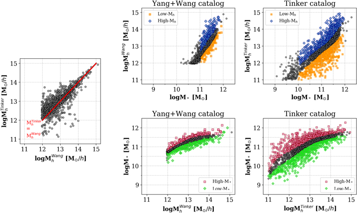
Figure 1. Comparison between the Mh
measured by Wang et al. (2016) and Tinker (2021) for our passive centrals. The  M
M
 line is shown in red. Right: SHMR for passive centrals in the two catalogs. We define our subsamples based on the independent property and SHMR. At fixed M* (top panels), high-Mh
centrals are shown in blue and low-Mh
centrals in orange. At fixed Mh
(bottom panels), high-M* centrals are shown in red and low-M* centrals in green. Galaxies in regions of the SHMR with narrow dynamic range were not included in the analysis (gray). We also excluded galaxies between the 33rd and 66th percentiles in M*-to-Mh
ratio.
line is shown in red. Right: SHMR for passive centrals in the two catalogs. We define our subsamples based on the independent property and SHMR. At fixed M* (top panels), high-Mh
centrals are shown in blue and low-Mh
centrals in orange. At fixed Mh
(bottom panels), high-M* centrals are shown in red and low-M* centrals in green. Galaxies in regions of the SHMR with narrow dynamic range were not included in the analysis (gray). We also excluded galaxies between the 33rd and 66th percentiles in M*-to-Mh
ratio.
Download figure:
Standard image High-resolution imageTable 1. Number of Central Galaxies per Sample
| M*[M⊙] = | 1010 − 1010.5 a | 1010.5 − 1011 a | 1011 − 1011.5 | 1011.5 − 1012 | Out of Range | Total |
|---|---|---|---|---|---|---|
| Yang+Wang | 7 | 267 | 523 | 153 | 2 | 952 |
| Yang+Wang low-Mh | 0 | 0 | 174 | 48 | ⋯ | 222 |
| Yang+Wang high-Mh | 0 | 0 | 172 | 51 | ⋯ | 223 |
| Tinker | 211 | 514 | 948 | 412 | 132 | 2217 |
| Tinker low-Mh | 70 | 188 | 317 | 128 | ⋯ | 703 |
| Tinker high-Mh | 70 | 143 | 353 | 148 | ⋯ | 714 |
| Mh [M⊙/h] = | 1011 − 1012 a | 1012 − 1013 | 1013 − 1014 | 1014 − 1015 | Out of Range | Total |
| Yang+Wang | 27 | 517 | 358 | 49 | 1 | 952 |
| Yang+Wang low-M* | 0 | 170 | 120 | 19 | ⋯ | 309 |
| Yang+Wang high-M* | 0 | 172 | 113 | 15 | ⋯ | 300 |
| Tinker | 329 | 888 | 860 | 139 | 1 | 2217 |
| Tinker low-M* | 109 | 297 | 265 | 45 | ⋯ | 716 |
| Tinker high-M* | 112 | 310 | 301 | 50 | ⋯ | 773 |
Note.
a These bins were not considered as a result of the narrow dynamic ranges in Mh or M* (Figure 1).Download table as: ASCIITypeset image
2.5. Tinker Halo Masses
Group-finding algorithms, like the one described in Section 2.4, are affected by several issues. By not breaking down galaxy samples into star-forming and quiescent subsamples, they can fail to reproduce the fraction of quenched satellite galaxies and misestimate by an order of magnitude Mh (Campbell et al. 2015). Some of these shortcomings can be tackled by calibrating the free parameters of the group finder with real data instead of mock catalogs. In this paper, we work with the group finder by Tinker (2020), which uses observations of color-dependent galaxy clustering and total satellite luminosity for calibration.
In the self-calibrating halo-based galaxy group finder by Tinker (2020), the probability of a galaxy being a satellite depends on galaxy type and luminosity. This dependence is quantified by 14 different parameters that are calibrated until the best-fitting model is found. First, a starting value for the parameters is adopted and the group finder is run until the fraction of red and blue satellites match the input data set. The assigned groups and halo masses are then used to populate the Bolshoi–Planck simulation (Klypin et al. 2016) and predict galaxy clustering and the total satellite luminosity. These predictions are compared to observational measurements to quantify the adequacy of the model. The process is then repeated until the best-fitting model is found.
This algorithm was applied to SDSS galaxies in Tinker (2021). Compared to the data set available to Yang et al. (2005, 2007), Tinker (2021) had access to deeper photometry from the DESI Legacy Imaging Survey (DLIS; Dey et al. 2019). This is quite important, since good accounting of group and galaxy M* is key to properly constraining Mh (Bernardi et al. 2013; Wechsler & Tinker 2018). As a result, the SDSS group catalog by Tinker (2021) is an improvement in both data set and algorithm.
Despite improvements, the approach by Tinker (2020) still has limitations. Like all group-finding algorithms, it is susceptible to central galaxy misidentification. It also assumes that the amount of light in satellite galaxies is a function of halo mass only, and its implementation on SDSS data fails to match the clustering of faint quiescent galaxies (Tinker 2021). There is also room for further freedom in how the algorithm fits the data, in particular for taking into account secondary correlations between galaxy and halo properties (Tinker 2021).
The self-calibrating halo-based galaxy group finder applied to SDSS is publicly available.
34
We downloaded the catalog and cross-matched with our sample of quenched systems. We selected all galaxies with satellite probabilities lower than 0.1 and obtained a sample with 2217 passive central galaxies (see Table 1). The Mh
measured by Tinker and Yang+Wang are compared in the left panel of Figure 1. The right panel shows the SHMR using our M* and  , which extends down to M* ∼ 1010
M⊙ (M
, which extends down to M* ∼ 1010
M⊙ (M
 M⊙). Figure 2 shows that the average number of satellites per halo monotonically increases with
  .
.
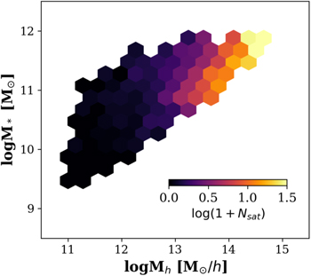
Figure 2. Number of satellite galaxies per halo as a function of Mh and M* in the Tinker (2020, 2021) catalog. At fixed M*, centrals in high-Mh halos tend to have more satellites than centrals in low-Mh halos.
Download figure:
Standard image High-resolution image3. Methodology
3.1. Sample Definitions
The correlation between the M* and Mh of central galaxies has significant scatter, some of which is thought to be intrinsic (e.g., Xu & Zheng 2020). This would imply that the stellar masses of central galaxies are determined not uniquely by the mass of their halos but also by secondary properties (e.g., Zentner et al. 2014). In consequence, the SHMR is a very useful tool for testing the mechanisms driving the galaxy–halo connection (e.g., Leauthaud et al. 2017). The purpose of this work is to probe these mechanisms through the analysis of galaxy stellar populations.
Figure 1 shows the SHMR for our sample of centrals according to both environmental catalogs. We computed the 33rd and 66th percentiles in M*-to-Mh ratio as a function of M* to define two subsamples. High-Mh centrals are those that reside in high Mh for their M* and are shown in blue. Low-Mh centrals, on the other hand, reside in low-Mh halos for their M* and are shown in orange. In equation form,

To quantify correlations at fixed Mh , we also computed the 33rd and 66th percentiles in M*-to-Mh ratio as a function of Mh . High-M* centrals have high M*-to-Mh ratios, whereas low-M* centrals have low M*-to-Mh ratios. Put in an equation,

Galaxies between the 33rd and 66th percentiles in M*-to-Mh ratio were not used and are shown as gray points in Figure 1. Since the distribution of centrals in M*-to-Mh ratio as a function of M* or Mh is rather flat, no subsample is biased as a result of uncertainties in M* or Mh . Note that the sample membership of a given galaxy depends on the environmental catalog, since our classification scheme is based on Mh . The number of galaxies in every M* and Mh bin for the two environmental catalogs is presented in Table 1. Due to the narrow dynamic range in Mh with the Yang+Wang catalog for M* < 1011 M⊙, the corresponding bins were not included in the analysis (see Table 1). The average number of satellites per halo (Nsat) for every subsample is plotted in Figure 2. At fixed M*, Nsat correlates with Mh .
3.2. Co-addition and Stacking of Spectra
The spectral precision needed by our stellar population analysis requires high-S/N (≳50) spectra (e.g., Conroy et al. 2014). Thus, we first co-added the MaNGA spectra within every galaxy following a radial binning scheme. We then computed the median of these co-additions to generate galaxy stacks for every subsample. The co-addition and stacking steps are described below.
For every galaxy, we associated galactocentric distances all spaxels by retrieving elliptical polar radii (R) from the DAP that account for the axis ratio of every object. We binned all the spaxels within every galaxy into the three annuli R = [0, 0.5]Re , [0.5, 1]Re , and [1, 1.5]Re . After masking sky-line residuals and spectra outside the wavelength range (3700 Å, 9200 Å) in the observed frame, the co-added spectra in every bin were co-added. To do this, we shifted every spectrum back to the rest frame using the stellar systemic velocity (v*) maps computed by the DAP with a Voronoi binning scheme that aims for a minimum S/N of 10 bin–1. We did not convolve the spectra to a common σ* prior to stacking. We also masked all spaxels that were flagged as unusable by the DRP and DAP.
After co-addition, we ran pPXF (Cappellari & Emsellem 2004; Cappellari 2017) with the MILES Single Stellar Population (SSP) library (Vazdekis et al. 2010) on the resulting spectra to measure the co-added v* and σ*. Co-added v* showed values v* ≲ 1 km s−1, indicating that spectra were properly shifted back to the rest frame. We also ran Prospector (details in Section 3.4) to measure stellar mass surface density profiles for every galaxy.
After binning in M* and Mh (see Table 1), we stacked the spectra across every subsample in each of the four radial annuli. For stacking, all co-added spectra were convolved to σ* = 350 km s−1 and median normalized. This value is motivated by the maximum observed dispersion, and it mitigates line-strength variations caused by different Doppler broadening. Stacks were obtained by computing the median at each wavelength after removing the continuum. Errors on the stacks were quantified through Monte Carlo simulations of the stacking process that took into account the propagated errors. Two stacked spectra are shown in Figure 3 after all emission lines were masked. The dependence of the stacks on whether masking is performed before or after stacking is minimal.
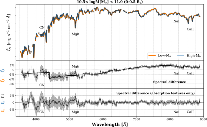
Figure 3. Top: stacked spectra of central galaxies at fixed M* that reside in low-Mh halos (orange) and high-Mh halos (blue). The data represent stacks within the central 0.5Re for M* = 1010.5 − 1011 M⊙ centrals. Middle: the high-Mh stack subtracted from the low-Mh stack with a fit plotted in black. Gray shading shows the error on this difference. Bottom: result of subtracting the fit from the spectral difference. This highlights variations in several absorption features, some of which help to break degeneracies between various stellar population parameters. The two subsets reveal significant differences in both spectral shape and absorption features. Requiring no model assumptions, this figure demonstrates that Mh has an impact on the stellar populations of passive central galaxies with the same M*.
Download figure:
Standard image High-resolution imageThe Appendix shows stacked spectra at multiple radii and Mh . We typically reach S/N > 200 at the centers and S/N > 100 in the outskirts. We find the spectral S/N of the stacks to show dependence on both the individual S/N and the total number of spectra. As a result, the highest M* and Mh stacks show the lowest spectral S/N of all bins by factors of ∼2.
3.3. Evidence for Environmental Differences
The top panel of Figure 3 compares the stacked spectra at the centers of high- and low-Mh centrals with M* = 1010 − 1010.5 M⊙. With M* held constant (see Section 3.1), any differences between the spectra in this comparison can be interpreted as environmental signatures. In this subsection, we describe our method for finding and highlighting these signatures.
We started by subtracting high-Mh stacks from low-Mh counterparts of the same M*. An example of the resulting spectral difference is shown in the middle panel of Figure 3. Then, to highlight variations in spectral features, we subtracted fits from the spectral differences. The result is shown in the bottom panel of Figure 3. Note how the spectral difference captures variations in both spectral shape and features. As we will show in Section 4, we find some significant environmental signatures at different M* and radii. This is evidence that Mh has an impact on the stellar populations of passive central galaxies at fixed M*.
For context, some abundance-sensitive features are labeled in this figure. Differences at these locations highlight the fact that environmental signatures can manifest because of differences in stellar age, metallicity, element abundances, and the IMF of central galaxies (Conroy et al. 2018). To inform our interpretation of these differences, we turned to stellar population fitting codes Prospector and alf.
3.4. Stellar Mass Surface Density Profiles with Prospector
We used the stellar population fitting code Prospector 35 (Leja et al. 2017; Johnson et al. 2021) on the co-added spectra to estimate stellar masses (Section 2.3) and stellar mass surface density (Σ*) profiles for all galaxies.
Prospector samples the posterior distribution for a variety of stellar population parameters and star formation history (SFH) prescriptions defined by the user. In this code, stellar population synthesis is handled by the code FSPS 36 (Conroy et al. 2009; Conroy & Gunn 2010). Our runs used the MILES stellar library (Sánchez-Blázquez et al. 2006), MIST isochrones (Dotter 2016; Choi et al. 2016), and Kroupa IMF (Kroupa 2001) as inputs. We adopted a nonparametric SFH with a continuity prior, which emphasizes smooth SFHs over time (Leja et al. 2019). As in Leja et al. (2019), we used the following time bins:
Our parameter space also included the optical depth of dust in the V band (Kriek & Conroy 2013), stellar mass, stellar velocity dispersion, and mass-weighted stellar ages and metallicities. To derive the posterior distributions, we used the Dynamic Nested Sampling package dynesty 37 (Speagle 2020).
3.5. Stellar Ages and Element Abundances with alf
We used the program alf to characterize the stellar populations in more detail. This code fits the absorption-line optical–near-infrared spectrum of old ( ≳1 Gyr) stellar systems (Conroy & van Dokkum 2012; Conroy et al. 2018). Unlike Prospector, alf allows us to fit for the abundances of multiple elements and the IMF. This comes at the cost of computation times that are longer by a factor of 100. alf is based on the MIST isochrones (Dotter 2016; Choi et al. 2016) and the empirical stellar libraries by Sánchez-Blázquez et al. (2006) and Villaume et al. (2017). Full spectral variations induced by deviations from the solar abundance pattern are quantified in the theoretical response functions (Conroy et al. 2018; Kurucz 2018). These allow alf to sample a multivariate posterior that includes the abundances of 19 elements (including C, N, O, Mg, and Fe).
We ran alf in “full” mode, which fits for a two-component SFH, stellar velocity dispersion, IMF, and the abundances of 19 elements. We adopted a triple power-law IMF with two free parameters. Power laws were fit in the ranges 0.08–0.5 M⊙ and 0.5–1 M⊙. The IMF slope was set to −2.35 in the range 1–100 M⊙ (Salpeter 1955). Posterior sampling was performed with emcee (Foreman-Mackey et al. 2013). We found our runs to fully converge under the default configuration, which is 1024 walkers, 104 burn-in steps, and 100-step chains. For this setup, alf took ∼100 CPU hours per spectrum to run.
With alf, we recover stellar velocity dispersions within 1% of the input value (σ* = 350 km s−1). We derived mass-weighted stellar ages by mass-weighting the posteriors of the two-component SFHs. The stellar ages measured by Prospector and alf show agreements within 2 Gyr. The most significant age differences between high- and low-Mh centrals are found by both codes. More subtle differences are only detected by alf (more details in Section 4). Following the approach of Lick indices, we use [Mg/Fe] as a proxy for [α/Fe] throughout (Johansson et al. 2012a; see Kirby et al. 2008 for other elements that can be used as tracers for [α/Fe]). Conversions from [X/H] to [X/Fe] assumed the correction factors in Schiavon (2007). The abundances measured by alf cannot be directly compared to the stellar metallicity reported by Prospector, since the latter only fits a scaled solar abundance pattern.
For estimating uncertainties on the fitted parameters, we adopted a three-step method that was iterated over 5 times. First, we bootstrapped the galaxies selected in the sample assignment step from Section 3.1. Then, we computed the stacked spectra for the corresponding bootstrapped galaxies as in Section 3.2. Lastly, we fit each stacked spectrum with alf. This resulted in five posterior distributions for every subsample in each stellar and halo mass bin. The five distributions were then folded in, such that the final posteriors account for uncertainties in both methodology and modeling. Some of the model fits and posterior distributions are shown in the Appendix.
4. Results
4.1. Empirical Spectral Differences with Environment
Using the methods in Section 3.3, we quantified differences between the spectra of centrals in high- and low-Mh halos. Our findings are plotted in Figure 4. The M* of the compared galaxies increases from left to right, with the top row displaying results for an inner bin of galactocentric radius and the bottom row results for an outer bin. Shaded contours show 1σ errors, which fully account for uncertainties in sample assignment and stacking. Absorption features that are deeper in low-Mh galaxies are negative, whereas features that are stronger in high-Mh galaxies are positive. We listed the stellar parameters that drive feature changes as quantified in the response functions by Conroy et al. (2018).
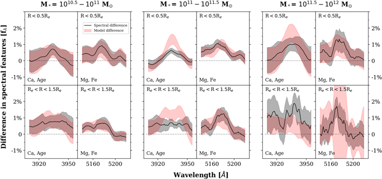
Figure 4. Differences in spectral features between low- and high-Mh centrals of the same M*. Positive difference indicates stronger absorption in high-Mh galaxies, with the 1σ error plotted in gray. Different panels show different spectral features for which we detect significant differences that are systematic with M* and radius. Stellar mass increases from left to right, galactocentric distance from top to bottom. Annotated are the stellar population parameters that dominate the strength of each feature. The red shading represents the 1σ posterior distribution of the best-fitting model spectra produced by alf. The alf posteriors reproduce the observed spectral differences well, although some model mismatch at the 1% level is apparent.
Download figure:
Standard image High-resolution imageAt all M* and radii, high-Mh centrals show stronger Mgb λ5172 absorption (Faber & Jackson 1976; Faber et al. 1985). Apart from being dominated by magnesium abundance, this spectral feature is also sensitive to iron enrichment. Another significant set of spectral differences are found around 4000 Å, which tend to be stronger in high-Mh centrals. These features are in a Ca-sensitive spectral region, as evidenced by the widely used Ca H and K, Ca λ4227, and Ca λ4455 spectral indices (e.g., Worthey et al. 1994; Tripicco & Bell 1995). Apart from being sensitive to the calcium abundance, features at these wavelengths are also sensitive to stellar age and overall metallicity.
The detection of these differences demonstrates that halos have an impact on the stellar populations of passive central galaxies that is secondary to the correlation between Mh and M*. We now turn to our results from stellar population fitting to attempt to interpret these results.
4.2. Integrated Measurements
To derive the mean stellar population properties within the galaxy, we averaged the radial profiles derived with alf (Section 3.5). The results are shown with M* and Mh as the controlling variable in the top and bottom panels of Figure 5, respectively. Measurements that used the Tinker catalog are plotted in circles, whereas those that used the Yang+Wang catalog are shown in the insets as triangles.
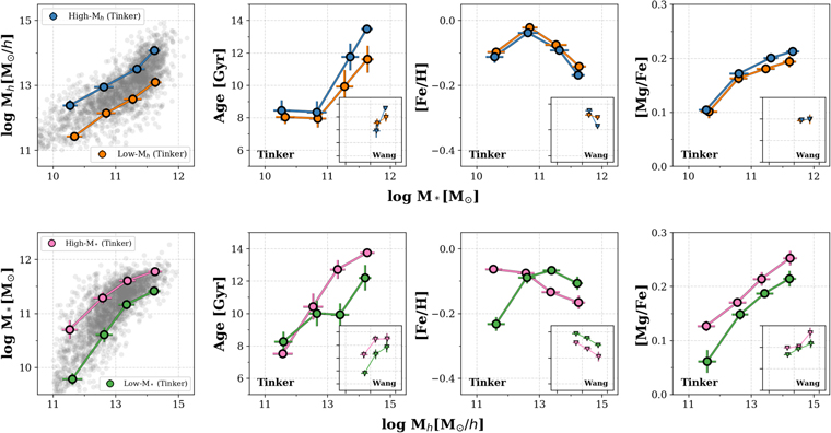
Figure 5. Stellar population parameters of passive central galaxies within 1.5Re as a function of M* (top) and Mh (bottom). Measurements that used the Tinker catalog for sample assignment are plotted in circles. Measurements that used the Yang+Wang catalog are shown in triangles. The stellar populations of passive centrals better correlate with M* than with Mh . Top: high-Mh centrals are older (3.6σ), have lower [Fe/H] (3.6σ), and show higher [Mg/Fe] (3.4σ) than low-Mh centrals. Bottom: for Mh > 1012 h−1 M⊙, the stellar populations of high-M* centrals are older (4.4σ), have lower [Fe/H] (5σ), and have greater [Mg/Fe] (4.4σ) than those of low-M* counterparts.
Download figure:
Standard image High-resolution imageTo first order, it is well known that stellar age and metallicity increase with the M* or central velocity dispersion of galaxies (Faber & Jackson 1976; Cid Fernandes et al. 2005; Gallazzi et al. 2005; Thomas et al. 2005, 2010; González Delgado et al. 2014; McDermid et al. 2015). While the top row of Figure 5 confirms this trend with age for the passive central galaxies in our study, we see that [Fe/H] decreases with M*. In the literature, the word “metallicity” refers to a weighted average of the abundance of various elements (i.e., a rescaling of the solar abundance pattern), whereas the [Fe/H] measurements that we derived with alf map the abundance of iron only. The decrease in [Fe/H] with M* for M* > 1011 M⊙ is likely the result of how the formation timescales of galaxies become more rapid as M* increases.
The plot in the top row, second column compares the stellar ages of low- and high-Mh centrals at fixed M*. With the Tinker catalog, we find low-Mh centrals to be younger than high-Mh counterparts by ∼1 − 2 Gyr. Differences between the [Fe/H] of low- and high-Mh centrals are also present, with high-Mh centrals showing lower [Fe/H] by ≲0.05 dex at all M*. High-Mh centrals also show slightly greater [Mg/Fe], especially for M* > 1011 M⊙. Figure 5 shows that the deeper absorption seen in high-Mh centrals (Figure 4) is primarily a result of their older ages and higher magnesium enhancement.
We can assign confidence levels to these results by computing the Bayes factor. As an example, we can consider the following two hypotheses: either high-Mh centrals are older, or low-Mh centrals are older. The Bayes factor is just the ratio between the marginalized likelihoods of the models since we are interested in adopting flat, uninformative priors. In equation form, the Bayes factor is equal to
Figure 5 indicates that for the first M* bin the stellar ages of the two subsamples are quite similar, and therefore  . On the other hand, high-Mh
centrals are significantly older in the highest-M* bin, and hence the associated Bayes factor is
. On the other hand, high-Mh
centrals are significantly older in the highest-M* bin, and hence the associated Bayes factor is  . If we assume that the two hypotheses cover all possible model options (i.e., that at least one of the subsamples is older), we can impose that the sum of the model probabilities is equal to 1 (e.g., Oyarzún et al. 2017). With this method, we conclude that high-Mh
centrals are older, have lower [Fe/H], and feature higher [Mg/Fe] than low-Mh
centrals with 3.6σ, 3.6σ, and 3.4σ confidence levels, respectively.
. If we assume that the two hypotheses cover all possible model options (i.e., that at least one of the subsamples is older), we can impose that the sum of the model probabilities is equal to 1 (e.g., Oyarzún et al. 2017). With this method, we conclude that high-Mh
centrals are older, have lower [Fe/H], and feature higher [Mg/Fe] than low-Mh
centrals with 3.6σ, 3.6σ, and 3.4σ confidence levels, respectively.
We can now invert this analysis and use Mh as the controlling variable. The results are shown in the bottom row of Figure 5 and indicate clear secondary behavior in the stellar population of galaxies with different values of M* at fixed Mh . We see that high-M* centrals are nearly always older. For Mh > 1012 h−1 M⊙, this difference can exceed 2 Gyr, has a significance of 4.4σ, and is clear in both halo catalogs. Differences in [Fe/H] show more complicated behavior that is dependent on Mh . For Mh < 1012 h−1 M⊙, high-M* centrals show higher [Fe/H] by as much as 0.2 dex (8σ). For Mh > 1012 h−1 M⊙, the difference reverses and [Fe/H] decreases with Mh (5σ). Significant differences are also observed in [Mg/Fe], with high-M* centrals showing greater [Mg/Fe] at all Mh (5.6σ) and for Mh > 1012 h−1 M⊙ (4.4σ) with both catalogs.
To help visualize the results across this multidimensional space, Figure 6 shows the SHMR colored by each of the stellar population properties we considered. This figure was made by fitting a two-dimensional, second-degree polynomial in M*–Mh space to the results from Figure 5. Note how stellar age and [Mg/Fe] vary not only with M* but also with Mh . On the other hand, [Fe/H] depends almost exclusively on M*.
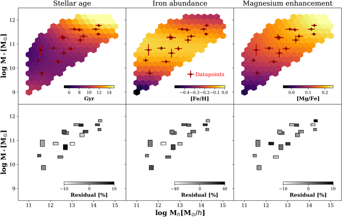
Figure 6. Top: the SHMR of passive centrals colored by stellar age, [Fe/H], and [Mg/Fe]. Values were derived by fitting two-dimensional polynomials in M*–Mh
space to the measurements from Figure 5 that adopted  (red data points). All parameters depend on both M* and Mh
. Bottom: residuals relative to the median value of the parameter in the SHMR.
(red data points). All parameters depend on both M* and Mh
. Bottom: residuals relative to the median value of the parameter in the SHMR.
Download figure:
Standard image High-resolution image4.3. The Stellar Population Profiles of Central Galaxies
We now look at the radial dependence of our derived measurements. The stellar population profiles at fixed M* are shown in Figure 7, with M* increasing from left to right. High-Mh profiles are shown in blue and low-Mh profiles in orange. The comparison at fixed Mh is shown in Figure 8, with high-M* centrals in magenta and low-M* centrals in green. The findings reported in this section apply to both catalogs, although only measurements using the Tinker catalog are shown to keep the figures simple.
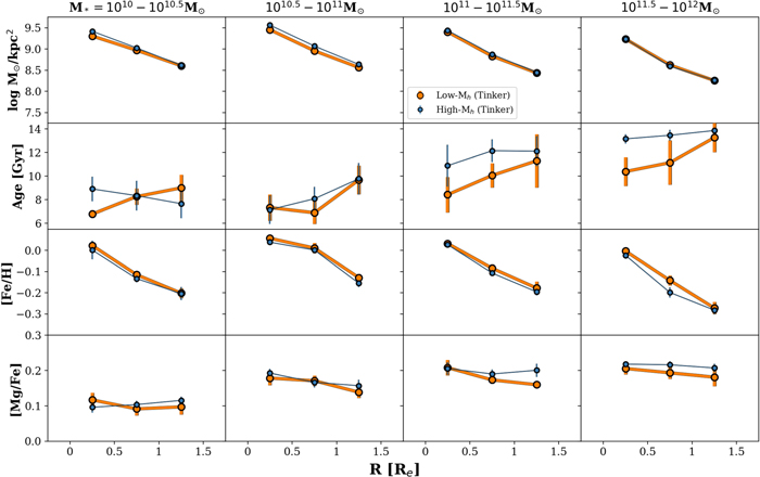
Figure 7. Stellar population profiles of low-Mh (orange) and high-Mh (blue) centrals at fixed M* with the Tinker catalog. From top to bottom, shown are stellar mass surface density, stellar age, [Fe/H], and [Mg/Fe]. Stellar mass increases from left to right. Low-Mh centrals have younger stellar populations at all radii for M* > 1011 M⊙ and higher [Fe/H] at all radii and all M* than high-Mh centrals.
Download figure:
Standard image High-resolution image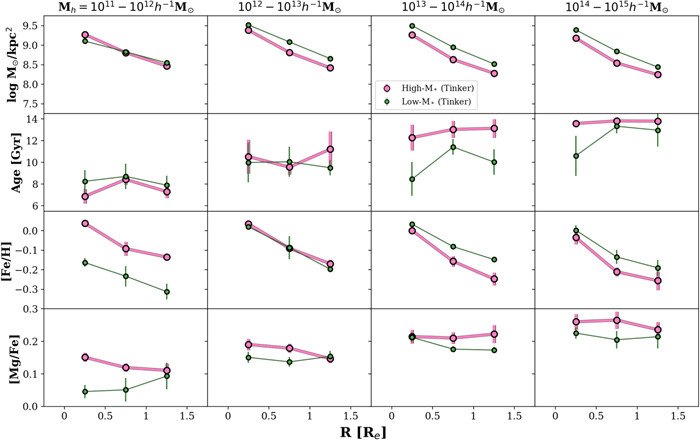
Figure 8. Stellar population profiles of high-M* (red) and low-M* (green) centrals at fixed Mh with the Tinker catalog. From top to bottom, shown are stellar mass surface density, stellar age, [Fe/H], and [Mg/Fe]. Stellar mass increases from left to right. Despite their lower Σ*, high-M* centrals are more massive owing to their much larger Re . For Mh > 1012 h−1 M⊙, high-M* centrals have stellar populations that are older, have lower [Fe/H], and show greater [Mg/Fe] than low-M* centrals at most radii.
Download figure:
Standard image High-resolution imageIn general, the stellar population profiles confirm the differences in normalization that we reported in Figure 5 and Section 4.2. We find stellar population differences to be rather constant with radius, indicating that no significant differences in profile shape are apparent between the subsamples. The stellar age and [Mg/Fe] profiles all tend to be flat, while the [Fe/H] profiles all fall with radius, as reported in previous work (e.g., Greene et al. 2015; van Dokkum et al. 2017; Alton et al. 2018; Parikh et al. 2018, 2019, 2021; Zheng et al. 2019; Lacerna et al. 2020).
The fact that parameter differences are mostly constant with radius indicates that the results in the integrated properties are not driven by outlier radial bins. This could have been more problematic in the outskirts, where the spectral S/N is a factor of two lower than at the centers (see the Appendix). The profiles would also reveal whether any trends in the integrated measurements are driven by standout physical behavior. For example, recent central star formation could also lower the mass-weighted stellar ages at the center, but we see no evidence for this either.
We therefore conclude that any variations in the shape of the stellar population profiles within 1.5Re must be very subtle. Processes like radial migration could contribute to “washing out” any subtle differences that might have been imparted by past events in the assembly history (Minchev et al. 2012; El-Badry et al. 2016). Moreover, the galactocentric distances probed in this paper are just inward of the radii at which the stellar metallicity profiles of nearby galaxies start to show flattening due to minor mergers and stellar accretion from satellite galaxies (Oyarzún et al. 2019).
5. Discussion
5.1. How Halo Mass Modulates the Stellar Populations of Passive Centrals at Fixed M*
In the two-phase scenario for galaxy evolution, the in situ formation of central galaxies is followed by a phase of ex situ growth through stellar accretion (Oser et al. 2010, 2012; Johansson et al. 2012b; Moster et al. 2013; Furlong et al. 2017). Recent observations of nearby massive galaxies provide support for this secondary phase. The stellar density profiles of massive galaxies at low redshift have faint, extended stellar envelopes that could have originated from late-time stellar accretion (Huang et al. 2013a, 2013b, 2018), as also identified locally in the Milky Way (e.g., Fernández-Trincado et al. 2019, 2020). Massive nearby galaxies also show flat stellar metallicity profiles beyond the Re , as would be expected if their outskirts assembled through minor mergers (Oyarzún et al.2019).
In Oyarzún et al. (2019), we showed that this transition in the shape of the stellar metallicity profiles becomes prominent in galaxies with stellar mass greater than M* = 1011 M⊙. Our estimates of the ex situ stellar mass fraction at Re are consistent with zero for M* < 1011 M⊙ and unity for M* > 1011 M⊙. A phase transition around M* = 1011 M⊙ also emerges in theoretical predictions. The baryon-to-star conversion efficiency is believed to peak around M* = 1010.5 M⊙ (e.g., Behroozi et al. 2013; Girelli et al. 2020), thus creating an inflection point in the SHMR (e.g., Moster et al. 2010; Posti & Fall 2021). As M* increases, the conversion efficiency decreases and mergers grow in importance (Rodriguez-Gomez et al. 2016; Rodríguez-Puebla et al. 2017). To first order, stellar mass that would have formed in the central galaxy at lower masses becomes increasingly locked up in satellites and the “intragroup” medium of host halos at higher masses. We can use these insights to inform our interpretation of Figures 5 and 7.
Focusing on lower-mass galaxies with M* < 1011 M⊙, we see that centrals in low-Mh halos have higher [Fe/H] within 1.5Re than centrals with the same M* in larger halos. The same trend was recovered by Greene et al. (2015) in the MASSIVE survey (Greene et al. 2013; though we should note that the opposite result was found by La Barbera et al. 2014 and Rosani et al. 2018; more in Section 5.2.3). This result can be interpreted two ways. First, it might imply that central galaxies in high-Mh halos more efficiently retained their gas throughout their star formation episodes. This could have led to rapid star formation, therefore enhancing their [Mg/Fe], which is precisely what we observe in Section 5. This Mg enhancement in high-Mh centrals was also detected by Scholz-Díaz et al. (2022), who also characterized the stellar populations of central galaxies, but with single-fiber SDSS spectroscopy.
Alternatively, we know by definition that at fixed M* low-Mh centrals also have higher M*-to-Mh ratios and lower numbers of satellites (see Figure 2). Perhaps our results are simply a sign of more extended central SFHs at lower halo masses, where lower virial temperatures and fewer satellites allow for longer periods of cold flow accretion (e.g., Dekel & Birnboim 2006; Zu & Mandelbaum 2016).
Before turning to the interpretation of our results toward M* > 1011 M⊙, we should emphasize that our sample binning and spectral S/N requirements in this work prevent us from studying the flattening of metallicity profiles in the low surface brightness outskirts of massive galaxies that were the subject of Oyarzún et al. (2019). The profiles in Figure 7 are mostly limited to the inner regions of galaxies, within ∼1.5Re . That said, we see in this work that Mh has an impact on the formation of passive galaxies, even at the centers of M* > 1011 M⊙ centrals. Though subtle, these signatures of halo-modulated evolution are significantly detected, as evidenced in Figures 3 and 4.
For M* > 1011 M⊙, the stars in high-Mh halo centrals are older than their counterparts in low-Mh halos. At these large M*, high-Mh centrals also have lower [Fe/H] and higher [Mg/Fe] at all radii. The fact that these differences are present at the centers and show little radial variation points to differences in in situ formation, as opposed to minor merger accretion at larger radii. In line with our interpretation at lower M*, a possible explanation is that low-Mh centrals continued forming stars over longer timescales. A later onset of quenching would yield younger stellar ages, higher [Fe/H], and lower [Mg/Fe] as measured today.
Given the more active merger history of high-M* galaxies, it is worth exploring the possibility that a fraction of the stars at the centers of M* > 1011 M⊙ centrals were accreted. To lower the [Fe/H] abundance and increase the stellar age in high-Mh centrals, accreted stars would have to be metal-poor and old. Oyarzún et al. (2019) argued that signatures of minor mergers are produced by the accretion of stellar envelopes that are more metal-poor than the inner regions of the central, giving credibility to this explanation. However, explaining why accreted stellar populations would be old is more challenging. The stellar ages of satellite galaxies rarely exceed 10 Gyr, even in halos as massive as Mh > 1014 h−1 M⊙ (Pasquali et al. 2010). Yet the stellar ages of high-Mh centrals can be as old as 12 Gyr for M* = 1011.5 M⊙.
Recently, Huang et al. (2020) exploited deep, wide-field imaging to measure individual ETG surface brightness profiles to R ∼ 150 kpc for a sample large enough that precise Mh estimates could be derived through galaxy−galaxy weak lensing. They found that, as a function of their host halo Mh , central galaxies contain more M* not only in their centers but also in their distant outskirts. If dry minor mergers are required to build those outskirts, does this mean that larger halos must be effective in suppressing star formation in both their central galaxies and the within-the-satellite population that will later merge onto those centrals? Further exploration of this question requires a direct comparison between the stellar population profiles of central and satellite galaxies, a subject we will return to in future work.
5.2. How M* Drives Evolution within Dark Matter Halos of Identical Mass
So far, we have discussed the influence of the host dark matter halo mass (Mh ) as a secondary, modulating variable in the formation and evolution of passive central galaxies at fixed M*. This approach follows a long line of literature seeking to understand the role of “environment” after controlling for luminosity or stellar mass (e.g., Dressler 1980; Kauffmann et al. 2004; Peng et al. 2010).
Our theoretical understanding of galaxy formation, however, begins by assuming an underlying distribution of evolving dark matter halos and then seeks to build physical models on top (see Benson et al. 2000; Moster et al. 2013; Somerville & Davé 2015). Acknowledging our imperfect ability in this paper to measure dark matter halos observationally (see Section 5.2.3), we nonetheless turn to a theory-minded perspective, in which halo mass is the primary variable. By studying trends with M* in bins of fixed Mh , we gain insight into the range of evolution that occurs within halos of fixed mass today.
Considering stellar age, [Fe/H], and [Mg/Fe] in nearly every mass bin, the bottom row of Figure 8 shows that the stellar populations of central galaxies at fixed Mh depend strongly on stellar mass. On the one hand, this result seems to be a familiar expression of how stellar populations depend on the luminosity of ETGs (see Renzini 2006 for a review). But when we remember that our trends are seen at fixed Mh , they are perhaps more surprising. In two halos of identical mass today, central galaxies with different M* have markedly different formation histories.
We discuss two physical interpretations of this result before concluding the discussion with an examination of potential observational biases.
5.2.1. Varying Conditions of Early Formation
Our first interpretation follows in the spirit of “monolithic collapse,” namely, that the early conditions (z ∼ 4) for gas accretion and mergers determine how the vast majority of stars in ETGs form. Rapid, intense formation leads to a greater stellar mass content (van Dokkum et al. 2009; Newman et al. 2010; Damjanov et al. 2011; Whitaker et al. 2012; Dekel & Burkert 2014; Zolotov et al. 2015). The number of stars formed in this early phase may therefore be largely independent of the progenitor halo properties, let alone the halo’s final mass at z = 0.
In this picture, certain halos would happen to host the conditions needed for gas-rich mergers that promote the early formation of massive central galaxies. These events would have to rapidly exhaust gas supplies to produce old and chemically enriched stellar populations today. Unfortunately, testing this scenario with stellar population profiles is challenging because the imprint of gas-rich mergers is hard to predict and sensitive to the initial conditions of the encounter (Kobayashi 2004).
We note, however, that at all Mh high-M* centrals are larger in size and show higher Σ* [M⊙/kpc] within ∼1Re compared to their low-M* counterparts (see Figure 8). Their initial “collapse” may have driven up such large central gas densities that the resulting deep potential wells limited the impact of feedback, driving runaway growth in M* (e.g., Matteucci 1994; Wellons et al. 2015). Such a period of collapse might leave kinematic and morphological signatures. Gas-rich major mergers might preserve the spin of the merger remnant, for example, giving rise to compact disks at z ∼ 2 (e.g., van der Wel et al. 2011) and so-called fast rotators (e.g., Graham et al. 2018). On the other hand, a more extended formation period followed by dry mergers might produce slow rotator galaxies (Naab et al. 2014).
In a sense, this general picture aligns with Section 5.1 in that stellar mass, and not the dark matter halo, emerges as the dominant variable that controls how the bulk of stars in passive centrals form. This would seem antithetical to current theoretical models, however, and inconsistent with a variety of observational studies emphasizing the importance of Mh , or at least proxies thereof (e.g., Σ1 kpc and σ*), in driving galaxy properties (Figures 3 and 4 of this paper and, e.g., Franx et al. 2008; Wake et al. 2012; Chen et al. 2020; Estrada-Carpenter et al. 2020).
5.2.2. Galaxy Assembly Bias
If a galaxy’s growth history is ultimately tied to its dark matter halo, then Figure 5 tells us that other halo parameters, beyond Mh , must play a role. These might include halo formation time and halo clustering (e.g., Gao et al. 2005; Wechsler et al. 2006), secondary properties that invoke the idea of “halo assembly bias.” By definition, this term encapsulates all correlations between halo clustering and the assembly histories of halos at fixed Mh (Mao et al. 2018; Mansfield & Kravtsov 2020). For example, dark matter halos that assembled early tend to be more strongly clustered than counterparts that assembled at lower redshift (Gao et al. 2005; Contreras et al. 2019), especially for Mh < 1013 h−1 M⊙ (Li et al. 2008).
The strong statistical relationship between halos and the galaxies they host (e.g., Leauthaud et al. 2017) has motivated predictions for how halo assembly bias might impact galaxy formation. Croton et al. (2007) used semianalytic models to predict that halo formation time should correlate with galaxy luminosity at fixed Mh . In a halo mass bin of Mh = 1014 − 1015.5 h−1 M⊙, they found that bright centrals formed in those halos that had mostly assembled by z ∼ 1, whereas fainter centrals were associated with halos that assembled later (z ∼ 0.5). Zehavi et al. (2018) expanded on this result, predicting a dependence of central M* on halo formation time at fixed Mh .
An implied secondary dependence of stellar mass growth on halo age has also been studied with semiempirical models. Bradshaw et al. (2020), for example, report factor of ∼3 differences in “central” M* between the 20% youngest and oldest halos at fixed halo mass above Mh > 1013 M⊙ as modeled in the UniverseMachine (UM; Behroozi et al. 2019). This difference in M* and age (of approximately 1–2 Gyr) is similar to our results in the two bottom left panels of Figure 5.
A galaxy assembly bias signal is also predicted in cosmological hydrodynamic simulations like EAGLE (Crain et al. 2015; Schaye et al. 2015; Matthee et al. 2017; Kulier et al. 2019) and Illustris (Vogelsberger et al. 2014; Nelson et al. 2015; Xu & Zheng 2020), where it is driven by the fact that halos in dense regions not only collapse earlier but also do so with higher halo concentrations (e.g., Wechsler et al. 2002; Zhao et al. 2009; Correa et al. 2015; Hearin et al. 2016b). That yields deeper potential wells (Matthee et al. 2017) and more efficient central star formation (e.g., Booth & Schaye 2010). For example, Matthee et al. (2017) found an order-of-magnitude variation in central M* at fixed halo mass below Mh ≲ 1012 M⊙. This variation correlates strongly with halo assembly time, which spans z = 0.6–3 (see their Figure 7).
In IllustrisTNG, galaxy assembly bias is strongly imprinted in galaxy observables. At fixed Mh , central galaxies that are dispersion dominated, are redder, are larger, and have higher M* are more strongly clustered, especially for Mh < 1013 h−1 M⊙ (Montero-Dorta et al. 2020). In addition, centrals in IllustrisTNG with high M*-to-Mh ratios exhausted their gas reservoirs earlier, thus quenching at higher redshifts (Montero-Dorta et al. 2021).
It is tempting to map these predictions to our observational results. At fixed Mh , high-M* centrals have stellar populations that are older, have higher [Mg/Fe], and show lower [Fe/H], revealing that they formed earlier and more rapidly. In the galaxy assembly bias scenario, this is a consequence of galaxy formation in older, highly concentrated halos. This explanation was also proposed by Scholz-Díaz et al. (2022) to explain why the same trends for stellar age and [Mg/Fe] are present in single-fiber spectra from SDSS.
Before we consider observational biases on this conclusion (Section 5.2.3), it is worth noting that there is disagreement among theoretical predictions for the detailed behavior of galaxy assembly bias. In the UM analysis, the secondary correlation with halo formation time is strongest for Mh ≳ 1014 M⊙ (Bradshaw et al. 2020; see also Croton et al. 2007). But Matthee et al. (2017) find that halo formation time in EAGLE has no effect above Mh ≳ 1012 M⊙, instead strengthening at lower masses (see also Kulier et al. 2019). Meanwhile, Zehavi et al. (2018) and Xu & Zheng (2020) find a correlation between halo age and M* that peaks around Mh ∼ 1012 h−1 M⊙ and mildly decreases in significance toward Mh ≳ 1013.5 h−1 M⊙. Uncertainties in late-time growth explain some of the discrepancy. In hydrodynamical simulations, the stochasticity of late mergers can wash out formation-time bias at high Mh (Matthee et al. 2017). The opposite happens in the UM because the bias here is driven by accreted stellar populations (Bradshaw et al. 2020). Halo age primarily influences the stellar mass that was accreted through mergers rather than the populations formed in situ.
Finally, we note that the more rapid formation of high-M* centrals, as inferred from the [Mg/Fe] and [Fe/H] measurements, is in agreement with the analysis by Montero-Dorta et al. (2021) in IllustrisTNG. However, it is in contrast with how high-M* centrals assemble in EAGLE, where they grow by forming stars over long timescales (Kulier et al. 2019). As Contreras et al. (2021) concluded in their comparison of different galaxy assembly bias models, the amplitude and behavior of the signal are strongly model dependent.
5.2.3. Systematic Errors and Assembly Bias Signal
Many studies have searched for signatures of galaxy assembly bias, and tentative detections have been reported, including correlations between halo concentration and the occupation fraction of centrals (Zentner et al. 2019; Lehmann et al. 2017), spatial clustering of galaxies (e.g., Berlind et al. 2006; Lacerna et al. 2014; Montero-Dorta et al. 2017), and galactic “conformity” (i.e., similarity in the physical properties of galaxies within a halo; Weinmann et al. 2006; Hearin et al. 2016a; Berti et al. 2017; Calderon et al. 2018; Mansfield & Kravtsov 2020). Unfortunately, systematic errors in the distinction between centrals and satellites, halo mass estimates, and other problems have called into question many of these results (see Campbell et al. 2015; Lin et al. 2016; Tinker et al. 2018; Wechsler & Tinker 2018).
Much of the concern in our work centers on the group catalogs we use to infer the host dark matter halo properties. Indeed, we show explicitly that the choice of group catalog can affect our results. For example, the Yang+Wang and Tinker catalogs disagree as to whether low-Mh centrals have higher or lower [Fe/H] than their high-Mh counterparts (see Figure 5). These discrepancies are also present in other work. La Barbera et al. (2014) and Rosani et al. (2018) used the Yang et al. (2007) catalog to find that high-Mh centrals have younger and more iron-enriched populations than low-Mh centrals. The opposite was found by Greene et al. (2015) with the catalog by Crook et al. (2007).
While we favor the new group catalogs from Tinker (2020, 2021), which are more sophisticated, self-consistent, and robust thanks to deeper imaging, systematic errors in Mh may significantly impact our conclusions. This is in large part because the Mh estimates depend, at least in part, on the M* of the central galaxy. In addition to counting satellite luminosity, the Tinker catalog also employs color and r-band light concentration when assigning Mh to an associated central galaxy. Our results indicate that high-M* centrals have higher central Σ*, the opposite of the expected bias with concentration. But they do have fewer satellites (apparent in Figure 2). This is expected because the central and satellite M* values must roughly add to a constant at fixed Mh . It is possible that the history of satellite accretion drives the stellar population trends we see, independently of the halo assembly history.
Finally, the identified sample of “central” galaxies (which is roughly identical in the Tinker and Yang+Wang catalogs) is both incomplete and contaminated (by actual satellite galaxies) in ways that likely depend on M* and inferred Mh . Disentangling these effects requires substantial mock observations that are beyond the scope of this paper.
Instead, in future work we can make progress by measuring observables associated with our subsamples that are independent of galaxy luminosity (i.e., independent of M*). For example, the assembly bias interpretation would be strengthened by a detection of different large-scale density signals on 10 Mpc scales for high- versus low-M* galaxies at fixed Mh . Likewise, we can exploit new, more accurate proxies for Mh (e.g., Bradshaw et al. 2020), eventually aiming to derive Mh estimates from stacked weak lensing.
6. Summary
We constructed a sample of over 2200 passive central galaxies from the MaNGA survey to study how their assembly histories depend on M* and Mh . We constrained the stellar populations of our galaxies to high precision through spectral stacking and characterization with the codes Prospector and alf. We also control for systematics in Mh estimation by comparing the outputs from the group catalogs by Yang et al. (2007), Wang et al. (2016), and Tinker (2020, 2021). Our findings can be summarized as follows:
- 1.At fixed M*, there are significant differences in the spectra of passive centrals as a function of Mh . These differences are present at all M* and we detect them at all radii (R < 1.5Re ). With no modeling involved, this shows that host halos have an impact on the formation of central galaxies.
- 2.To associate these spectral differences with stellar population variations, we turned to fitting with Prospector and alf. At fixed M*, centrals in more massive halos show older stellar ages, lower [Fe/H], and higher [Mg/Fe]. A possible explanation for this result is that centrals in massive halos more efficiently retained their gas, allowing for early and rapid formation. Alternatively, the fewer satellites in low-Mh centrals could allow for longer periods of cold flow accretion onto the central galaxy, resulting in more extended SFHs.
- 3.At fixed Mh , centrals with high M* have older stellar populations and formed in shorter timescales (low [Fe/H] and high [Mg/Fe]) than centrals with low M*. At first glance, this result might be expected given how the stellar populations of ETGs depend on M*. However, our results are among the first to distinguish these evolutionary trends at fixed Mh . We propose two different scenarios to explain these results:
Varying conditions of early formation: at fixed Mh , centrals that undergo gas-rich mergers can fuel rapid, intense star formation episodes followed by runaway growth in M*. This process of “enhanced collapse” leads to the formation of old, α-enhanced stellar populations.
Galaxy assembly bias: according to theory, central galaxies with high M*-to-Mh ratios assembled in early-forming, highly concentrated halos. Their gravitational potentials lead to early star formation, efficient metal retention, and rapid exhaustion of their gas reservoirs.
- 4.Though we use two group catalogs in our analysis, we are still sensitive to sample contamination and systematic errors in Mh estimation. Future work can improve on these difficulties by measuring observables that are independent of galaxy luminosity or by exploiting more accurate proxies for Mh .
We would like to thank the referee and statistics editor for the helpful comments and suggestions. We would also like to thank everyone at UC Santa Cruz involved in the installation and maintenance of the supercomputer Graymalkin, which was used to run alf on MaNGA spectra. This work made use of GNU Parallel (Tange 2018). G.O. acknowledges support from the Regents’ Fellowship from the University of California, Santa Cruz. K.B. was supported by the UC-MEXUS-CONACYT grant. J.G.F.-T. gratefully acknowledges the grant support provided by Proyecto Fondecyt Iniciación No. 11220340, as well as from ANID Concurso de Fomento a la Vinculación Internacional para Instituciones de Investigación Regionales (Modalidad corta duración) Proyecto No. FOVI210020 and from the Joint Committee ESO-Government of Chile 2021 (ORP 023/2021). M.A.F. acknowledges support by the FONDECYT iniciación project 11200107. This research made use of Marvin, a core Python package and web framework for MaNGA data, developed by Brian Cherinka, José Sánchez-Gallego, and Brett Andrews (MaNGA Collaboration, 2018). Funding for the Sloan Digital Sky Survey IV has been provided by the Alfred P. Sloan Foundation, the U.S. Department of Energy Office of Science, and the Participating Institutions. SDSS acknowledges support and resources from the Center for High-Performance Computing at the University of Utah. The SDSS website is www.sdss.org. SDSS is managed by the Astrophysical Research Consortium for the Participating Institutions of the SDSS Collaboration, including the Brazilian Participation Group, the Carnegie Institution for Science, Carnegie Mellon University, the Chilean Participation Group, the French Participation Group, Harvard-Smithsonian Center for Astrophysics, Instituto de Astrofísica de Canarias, Johns Hopkins University, Kavli Institute for the Physics and Mathematics of the Universe (IPMU) / University of Tokyo, Lawrence Berkeley National Laboratory, Leibniz Institut für Astrophysik Potsdam (AIP), Max-Planck-Institut für Astronomie (MPIA Heidelberg), Max-Planck-Institut für Astrophysik (MPA Garching), Max-Planck-Institut für Extraterrestrische Physik (MPE), National Astronomical Observatories of China, New Mexico State University, New York University, University of Notre Dame, Observatório Nacional/MCTI, The Ohio State University, Pennsylvania State University, Shanghai Astronomical Observatory, United Kingdom Participation Group, Universidad Nacional Autónoma de México, University of Arizona, University of Colorado Boulder, University of Oxford, University of Portsmouth, University of Utah, University of Virginia, University of Washington, University of Wisconsin, Vanderbilt University, and Yale University.
Appendix: Model Fits and Posterior Distributions
Figures A1, A2, A3, and A4 show some of the fits and composite posterior distributions for high-M* (red) and low-M* (green) centrals. Halo mass increases with figure number. Top panels show the continuum-subtracted stacks and best fits. Residuals are plotted underneath. The errors shown in gray include the jitter and inflated error terms implemented by alf. Black vertical lines delimit the wavelength ranges used for continuum subtraction.
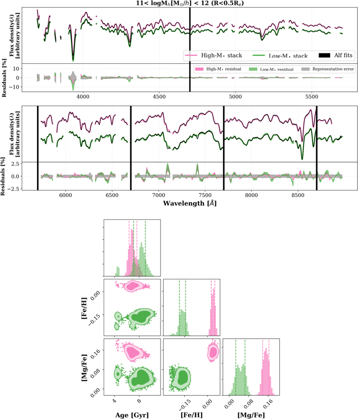
Figure A1. Top: best fits and residuals for the 11 < logMh [M⊙/h] < 12 bin (R < 0.5Re ). Bottom: posterior distributions. Details are given in the Appendix.
Download figure:
Standard image High-resolution image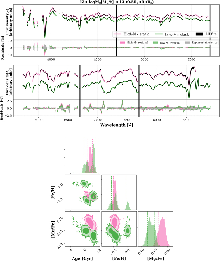
Figure A2. Top: best fits and residuals for the 12 < logMh [M⊙/h] < 13 bin (0.5Re < R < Re ). Bottom: posterior distributions. Details are given in the Appendix.
Download figure:
Standard image High-resolution image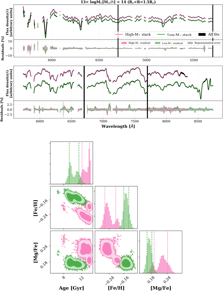
Figure A3. Top: best fits and residuals for the 13 < logMh [M⊙/h] < 14 bin (Re < R < 1.5Re ). Bottom: posterior distributions. Details are given in the Appendix.
Download figure:
Standard image High-resolution image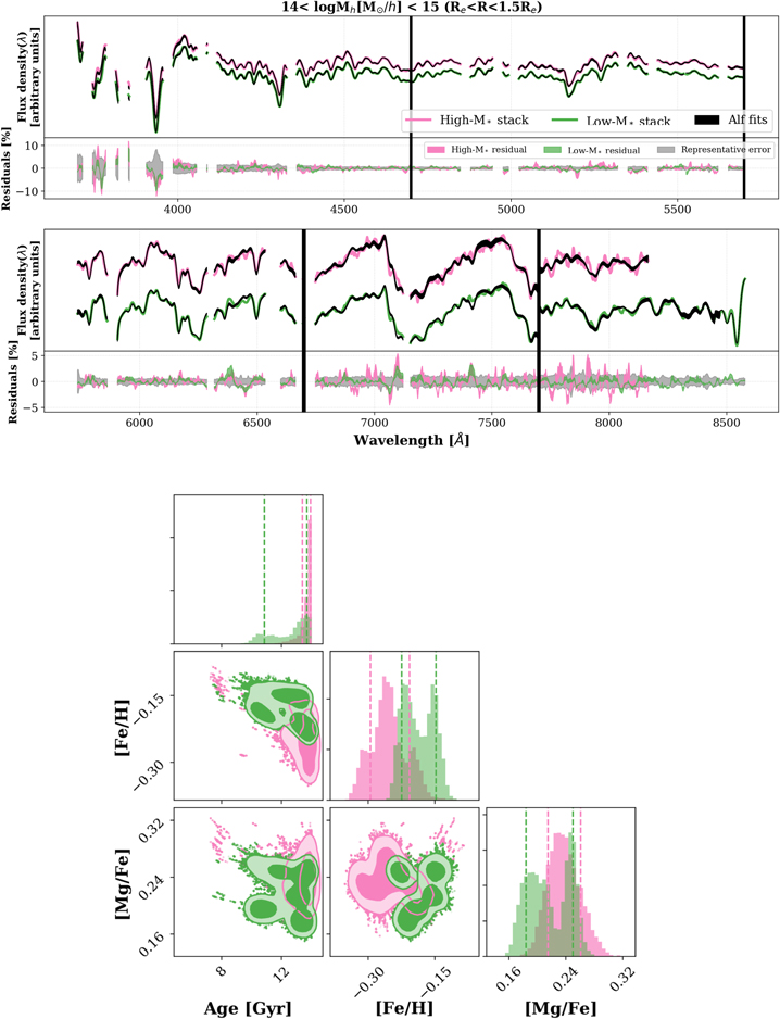
Figure A4. Top: best fits and residuals for the 14 < logMh [M⊙/h] < 15 bin (Re < R < 1.5Re ). Bottom: posterior distributions. Details are given in the Appendix.
Download figure:
Standard image High-resolution imageThe bottom panels show the posterior distributions of mass-weighted ages, [Fe/H], and [Mg/Fe] derived with alf for the two corresponding spectra. The assumptions used to derive these quantities from raw alf outputs are described in Section 3.5. We fitted for a two-component SFH, stellar velocity dispersion, IMF, and the abundances of 19 elements. Posterior sampling was performed with emcee (Foreman-Mackey et al. 2013).
Footnotes
- 30
- 31
- 32
- 33
- 34
- 35
- 36
- 37