Abstract
We present the discovery of 17 double white dwarf (WD) binaries from our ongoing search for extremely low mass (ELM) < 0.3 M⊙ WDs, objects that form from binary evolution. Gaia parallax provides a new means of target selection that we use to evaluate our original ELM Survey selection criteria. Cross-matching the Gaia and Sloan Digital Sky Survey (SDSS) catalogs, we identify an additional 36 ELM WD candidates with 17 < g < 19 mag and within the 3σ uncertainties of our original color selection. The resulting discoveries imply the ELM Survey sample was 90% complete in the color range −0.4 < (g − r)0 < −0.1 mag (approximately 9000 K < Teff < 22,000 K). Our observations complete the sample in the SDSS footprint. Two newly discovered binaries, J123950.370−204142.28 and J232208.733+210352.81, have orbital periods of 22.5 and 32 minutes, respectively, and are future Laser Interferometer Space Antenna gravitational-wave sources.
Original content from this work may be used under the terms of the Creative Commons Attribution 4.0 licence. Any further distribution of this work must maintain attribution to the author(s) and the title of the work, journal citation and DOI.
1. Introduction
This paper presents new low-mass WD observations designed to assess the completeness of the ELM Survey. The ELM Survey is a spectroscopic survey targeting extremely low mass <0.3 M⊙, He-core WDs. To form such low-mass WDs within the current age of the universe requires binary evolution (Iben 1990; Marsh et al. 1995). Different evolutionary pathways can form low-mass WDs, and both common-envelope and Roche-lobe overflow evolution channels contribute to the observed low-mass WD population (Istrate et al. 2016; Sun & Arras 2018; Li et al. 2019). The ELM Survey is responsible for the majority of known low-mass WDs and the discovery of over 100 detached double degenerate binaries (Brown et al. 2020a, 2020b; Kilic et al. 2021).
Importantly, WD binaries with periods P ≲ 1 hr are potential multimessenger sources detectable with both light and gravitational waves with the future Laser Interferometer Space Antenna (LISA; Amaro-Seoane et al. 2017). Theoretical binary population models predict that the majority of multimessenger WD binaries will contain low-mass, He-core WDs (Korol et al. 2017; Lamberts et al. 2019; Breivik et al. 2020; Thiele et al. 2021). Observational surveys provide an opportunity to anchor these population models with actual numbers. The difficulty is that observations are based on optical magnitude and color, not model parameters like WD mass or binary period. A complete and well-defined observational sample provides the best basis for comparison.
Gaia astrometry now provides a powerful means to target WDs. Gentile Fusillo et al. (2021) use Gaia early Data Release 3 (eDR3) to identify hundreds of thousands of high-confidence WDs over the entire sky. Pelisoli & Vos (2019) used Gaia DR2 to identify candidate low-mass WDs. The original ELM Survey target selection, for comparison, was made on the basis of magnitude and color using Sloan Digital Sky Survey (SDSS) passbands. Here, we use Gaia astrometry to identify extremely low mass (ELM) WD candidates in the SDSS footprint within 3σ of our original color selection criteria, and present the observational results.
We discuss the details of the target selection in Section 2. We use dereddened magnitudes and colors indicated with a subscript 0 throughout. In Section 3, we present the observations and derive physical parameters. These measurements complete the color-selected ELM Survey sample in the SDSS footprint. In Section 4, we discuss the ELM Survey completeness and compare it with other Gaia-based WD catalogs. We close by highlighting J1239−2041 and J2322+2103, which are among the shortest-period detached binaries known, and discuss the gravitational-wave properties of the full sample of 124 WD binaries published in the ELM Survey.
2. ELM WD Target Selection
The original ELM Survey used dereddened (u − g)0 color as a proxy for surface gravity to select candidate low-mass WDs. Normal  DA-type WDs differ from normal
  A-type stars by up to 1 mag in (u − g)0 color in the temperature range −0.4 < (g − r)0 < −0.1 (about 9000 K to 22,000 K) due to the effect of surface gravity on the Balmer decrement in the spectrum of the stars (Brown et al. 2012b). This region of color space thus provides an efficient hunting ground for
  ELM WDs.
Color selection does not identify all possible ELM WDs, however, because of inevitable confusion with background halo A-type stars and foreground DA WDs with similar colors. During the course of the ELM Survey, we learned that the color selection becomes inefficient at <9000 K temperatures, or (g − r) > −0.1 mag, where the hydrogen Balmer lines lose their sensitivity to temperature and gravity. Low-mass WDs at <9000 K temperatures exist, but subdwarf A-type stars are 100 times more common at these temperatures (Kepler et al. 2015, 2016). Subdwarf A-type stars are mostly field blue stragglers and metal-poor halo stars (Brown et al. 2017; Pelisoli et al. 2017, 2018a, 2018b, 2019; Yu et al. 2019).
Fortunately, ELM WDs also have distinctive ∼0.1 R⊙ radii that fall in between normal ∼0.01 R⊙ DA WDs and ∼1 R⊙ A-type stars. These radii mean ELM WDs are found in a distinct range of absolute magnitude at a fixed color (temperature). Gaia now provides a direct means of selecting ELM WD candidates on the basis of parallax.
To test the ELM Survey completeness for low-mass WDs, we select ELM WDs using Gaia astrometry in the SDSS footprint as described below. Our spectroscopic observations began with Gaia DR2, and then transitioned to using Gaia eDR3 when it became available. We consider the results of both Gaia data releases.
2.1. Matching SDSS to Gaia DR2
Our initial approach was to crossmatch a wide range of stars with possible low-mass WD colors in SDSS against the Gaia DR2 catalog, so that we properly sample the SDSS footprint. SDSS provides ugriz photometry for about 10,000 deg2 of the northern hemisphere sky, mostly located at high Galactic latitudes ∣b∣ ≳ 30°.
We use SDSS DR16 photometry (Ahumada et al. 2020), which is identical to SDSS DR13 values used by the Gaia Collaboration. We correct all magnitudes for reddening using values provided by SDSS. Since our WDs have a median distance of 1 kpc, and background halo stars are even more distant, applying the full reddening correction is important for accurate color selection.
We began with a simple, broad color cut for blue stars. We select stars from SDSS DR16 with clean photometry (clean=1), g-band extinction <1 mag, and colors in the ranges −0.5 < (u − g)0 < 2.0 mag, −0.6 < (g − r)0 < 0.2 mag, and −0.75 < (r − i)0 < 0.25 mag and errors < 0.15 mag in (g − r)0 and < 0.2 mag in (u − g)0 and (r − i)0. The result of our query is 578,883 stars in the magnitude range 15 < g0 <20 mag.
We then performed an exploratory 10″ radius positional crossmatch with Gaia DR2. The exploratory crossmatch yields 577,253 matches, 16,680 of which are duplicates and 10,469 of which have no parallax or proper motion. Accounting for proper motion, we find that a 10.7 yr difference in epoch minimizes the position residuals for the blue stars, consistent with the mean epochs of SDSS and Gaia DR2.
Finally, we perform a clean crossmatch between SDSS and Gaia DR2. We require ruwe < 1.4, astrometric_n_good_obs_al > 66, and duplicated_source = 0 following the guidance of Lindegren et al. (2018). Our goal is to end up with a clean set of low-mass WD candidates, even if the ruwe cut may select against wide binaries like HE 0430−2457 (Vos et al. 2018). We accept objects that match within 1″ in position, corrected for 10.7 yr of proper motion, and that match within 1 mag between the Gaia G band and the average SDSS g + r band magnitude. We reject objects with no parallax or proper motion. This crossmatch yields astrometry for 543,534 blue SDSS stars, 94% of the original sample.
2.2. Matching Gaia eDR3 to SDSS
Following the release of Gaia eDR3, which has improved completeness for faint blue stars and 2× better astrometric errors than Gaia DR2, we transitioned to using Gaia’s best neighbor crossmatch with SDSS. This approach bases the selection on the Gaia catalog, not on the SDSS catalog, and so imposes an unseen astrometric figure of merit to the target selection. The advantage is that the Gaia best neighbor crossmatch makes use of the full five-parameter astrometric covariance matrix.
Starting with the same list of 578,833 blue SDSS stars, we use the gaiaedr3.sdssdr13_best_neighbor catalog to find Gaia eDR3 matches for 99.9% of the stars. We reject 3063 objects with no parallax, with matched positions that differ by >1″, or with number_of_mates > 0. We then create a clean catalog by applying the Gentile Fusillo et al. (2021) data quality cuts for high Galactic latitude white dwarfs, 5 excluding the parallax_over_error and pm_over_error criteria. We will do our own parallax and proper motion selection in the next sections. The final Gaia eDR3 crossmatch catalog contains clean astrometry for 567,769 blue SDSS stars, 98.4% of the original sample.
With the Gaia crossmatch in hand, we are ready to make various cuts of ELM WD candidates beyond the original ELM Survey. Gaia eDR3 astrometry supersedes Gaia DR2 in accuracy and precision, so we use Gaia eDR3 values throughout this paper.
2.3. ELM WD Candidates: Photometric Selection
We consider the apparent magnitude range 17 < g < 19 mag to maximize our volume for finding ELM WDs. We find that Gaia parallax is reliable to around 19 mag for our targets (see Section 2.4). We adopt −0.4 < (g − r)0 < −0.1 mag to fix the temperature range to approximately 9000 K to 22,000 K and avoid subdwarf A-type stars.
Our first ELM WD selection is based on (u − g)0 color. For reference, Figure 1 plots (u − g)0 versus (g − r)0 for every star in SDSS with 17 < g < 19 mag and E(V − B) < 0.1 mag. The lower band of dots are normal A-type stars: halo blue stragglers and blue horizontal branch stars. The upper band of dots are normal DA-type WDs, stars with the same temperatures but much higher gravities. ELM WDs fall in between. Magenta lines plot Althaus et al. (2013) evolutionary tracks for 0.16, 0.19, and 0.32 M⊙ WDs (Figure 1). Blue lines mark the approximate color selection of the HVS Survey (Brown et al. 2012a) and the ELM Survey (Brown et al. 2012b), which together formed the basis for our WD observations. Solid blue diamonds are the previously published clean ELM sample with 17 < g < 19 mag minus J0935+4411, a  ELM WD binary that was not selected by color (Kilic et al. 2014).
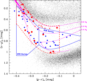
Figure 1. Color–color plot for every star in SDSS with 17 < g < 19 mag. For guidance, magenta lines plot theoretical 0.16, 0.19, and 0.32 M⊙ WD tracks (Althaus et al. 2013). Blue lines mark the approximate color selection of the HVS Survey and ELM Survey; blue diamonds mark previously published ELM WD binaries with 17 < g < 19 mag. Red dashed lines mark the new color selection, red crosses mark new ELM WD candidates, and red stars mark new ELM WD binaries.
Download figure:
Standard image High-resolution imageThe median SDSS (u − g)0 error at g = 19 mag is 0.038 mag. Thus, to test the ELM Survey completeness, we consider the 0.32 M⊙ WD track that is about 0.1 mag (3σ) beyond the original color cut. A polynomial fit, valid over −0.4 < (g − r)0 < −0.1 mag, yields (u − g)0 = 0.535 + 1.67(g − r)0
 . We use this line as our (u − g)0 color cut, bounded by the same line 0.5 mag redder in (u − g)0. The dashed red line in Figure 1 plots the color selection. There are 3094 candidates 17 < g < 19 mag in this color selection region. The large number of candidates reflects the overlap with the main locus of WDs in color space.
2.4. ELM WD Candidates: Parallax Selection
We can also select ELM candidates on the basis of Gaia parallax, independent of (u − g)0 color. Our second approach is to use Gaia parallax to calculate absolute g-band magnitude  , where π is in mas and corrected for the global Gaia parallax zero-point of −0.017 mas (Lindegren et al. 2021). We do not bother with higher-order zero-point corrections because the low-mass WD candidates have order-of-magnitude larger ± 0.17 mas median parallax errors. We consider the identical magnitude range 17 < g < 19 mag and temperature range −0.4 < (g − r)0 < −0.1 mag, and require parallax_over_error > 3.
For reference, Figure 2 plots Mg versus (g − r)0 for every star in SDSS with 17 < g < 19 mag. The lower band of dots are normal WDs, intrinsically faint foreground objects with Mg ≳ 10 mag. The upper cloud of dots is A spectral-type stars in the halo, intrinsically luminous background objects. ELM WDs fall in between. Magenta lines plot the same Althaus et al. (2013) evolutionary tracks for 0.16, 0.19, and 0.32 M⊙ WDs as before (Figure 2). For the sake of clarity, we clip the shell flash loops in the 0.19 M⊙ track that briefly jump to high temperature and luminosities. Blue stars mark previously published ELM Survey discoveries with 17 < g < 19 mag.
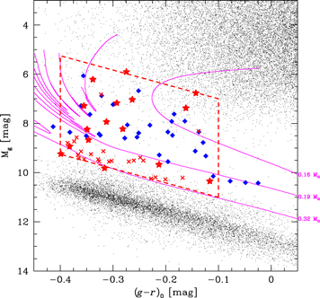
Figure 2. Absolute g-band magnitude computed from Gaia eDR3 parallax vs. dereddened (g − r)0 color for every star in SDSS with 17 < g < 19 mag. Magenta lines plot theoretical 0.16, 0.19, and 0.32 M⊙ WD tracks (Althaus et al. 2013); discontinuities are where we clip large excursions due to shell flashes in the 0.19 M⊙ track for the sake of clarity. Symbols are the same as in Figure 1. Red dashed lines mark the Gaia eDR3 selection. Red stars outside the dashed line were selected with Gaia DR2.
Download figure:
Standard image High-resolution imageIn Gaia eDR3, the median absolute magnitude error at g = 19 mag is 0.14 mag in our (u − g)0 cut (Figure 1). The median error is substantially worse (parallax_over_error = 0.3) outside of our (u − g)0 cut because of the large number of distant halo stars at similar temperatures. Thus, we consider the 0.32 M⊙ track that sits 1 mag below the faintest ELM Survey discovery, the same track that we used for the color selection. A linear fit, valid over −0.4 < (g − r)0 < −0.1 mag, yields Mg = 11.58 + 5.83(g − r)0. We use this line as our Mg cut, bounded by the same line 4 mag more luminous (smaller absolute magnitude) in Mg , as seen by the dashed red line in Figure 2. There are 192 candidates in this Mg selection region, 57 of which are in common with the (u − g)0 selection.
2.5. ELM Candidates: Optional Reduced Proper Motion Selection
Parallax provides a powerful but not a perfect selection criterion. Given Gaia measurement errors, WDs more distant than about 1 kpc become confused with halo stars on the basis of parallax alone. Proper motion provides an independent constraint. Given that halo stars are an order of magnitude more distant than ELM WDs, we can use reduced proper motion as an optional third selection criteria.
We compute g-band reduced proper motion  , where μ is the Gaia proper motion in mas yr−1. In Gaia eDR3, the median reduced proper motion error at g = 19 mag is 6% within our color cut. The precision is deceptive, however, as the intrinsic velocity dispersion of stars causes overlap in reduced proper motion space.
For reference, Figure 3 plots Hg versus (g − r)0 for every star in SDSS with 17 < g < 19 mag. The lower cloud of dots is normal WDs, nearby objects that exhibit larger proper motions than more distant stars of the same temperature. The upper clouds of dots are A spectral-type stars in the halo. ELM WDs fall approximately in between the foreground WDs and background halo stars, but with considerable spread. The problem is that known ELM WDs are a mix of disk and halo populations, and so exhibit a large spread in reduced proper motion space.
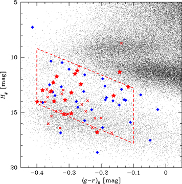
Figure 3. Reduced proper motion Hg computed from Gaia eDR3 proper motions vs. dereddened (g − r)0 color for every star in the SDSS with 17 < g < 19 mag. Symbols are the same as in Figure 1. Red dashed lines mark a possible selection that we do not use because of its poor efficiency.
Download figure:
Standard image High-resolution imageWe initially considered an empirical reduced proper motion selection 14 + 12(g − r)0 < Hg < 19 + 12(g − r)0 that includes previously published discoveries and minimizes the contribution of background halo stars (Figure 3). There are 5267 candidates in this Hg selection. However, the Hg selection has substantial overlap with the population of normal WDs, and legitimate ELM WDs are excluded. Given the inefficiency of the Hg selection compared to the other selection criteria, we do not consider it further.
2.6. Final Selection
Parallax selection provides the most efficient means for identifying low-mass WDs candidates with minimal contamination from foreground and background sources, followed by color selection. We combine the parallax and color selection to optimize our observing program.
Fifty-seven objects jointly satisfy the Gaia eDR3 parallax and SDSS color selection criteria with 17 < g < 19 mag. These objects are the highest-probability ELM WD candidates in the SDSS footprint. Table 1 presents the list. We include three additional objects (J0130−0530, J0820+4543, and J2151+2730) in Table 1 that were selected and observed using Gaia DR2 but do not satisfy the Gaia eDR3 parallax cut (i.e., the three objects that fall just outside selection region in Figure 2). We include them here for completeness.
Table 1. Measured and Derived WD Parameters
| Object | R.A. | Decl. | Pub | Bin | g0 | (g − r)0 | (u − g)0 | Teff |

| Mass | Mg | dspec | plx | Gaia eDR3 Source ID |
|---|---|---|---|---|---|---|---|---|---|---|---|---|---|---|
| (h:m:s) | (d:m:s) | (mag) | (mag) | (mag) | (K) | (cm s−2) | (M⊙) | (mag) | (kpc) | (mas) | ||||
| J0101+0401 | 1:01:28.690 | 4:01:59.00 | 0 | 1 | 17.219 ± 0.017 | −0.143 ± 0.033 | 0.993 ± 0.035 | 9284 ± 120 | 5.229 ± 0.089 | 0.188 ± 0.013 | 6.74 ± 0.26 | 1.245 ± 0.321 | 0.7958 ± 0.0981 | 2551884196495171712 |
| J0116+4249 | 1:16:00.832 | 42:49:38.32 | 0 | 1 | 18.337 ± 0.016 | −0.293 ± 0.020 | 0.634 ± 0.034 | 12968 ± 180 | 5.058 ± 0.045 | 0.256 ± 0.028 | 5.07 ± 0.15 | 4.506 ± 0.702 | 0.5682 ± 0.1794 | 373358998783703808 |
| J0130−0530 | 1:30:15.918 | −5:30:25.72 | 0 | 1 | 18.894 ± 0.032 | −0.293 ± 0.046 | 0.365 ± 0.050 | 14727 ± 120 | 5.420 ± 0.025 | 0.299 ± 0.053 | 5.47 ± 0.25 | 4.834 ± 1.233 | −0.0249 ± 0.2712 | 2479121368826845568 |
| J0745+2104 | 7:45:00.527 | 21:04:31.37 | 0 | 1 | 18.578 ± 0.013 | −0.399 ± 0.025 | 0.016 ± 0.027 | 22614 ± 290 | 7.329 ± 0.041 | 0.397 ± 0.016 | 9.21 ± 0.08 | 0.747 ± 0.059 | 1.3408 ± 0.2521 | 672983820089822464 |
| J0806−0716 | 8:06:50.022 | −7:16:36.11 | 0 | 1 | 18.065 ± 0.011 | −0.312 ± 0.016 | 0.652 ± 0.031 | 12374 ± 160 | 6.109 ± 0.041 | 0.203 ± 0.027 | 8.01 ± 0.16 | 1.027 ± 0.167 | 0.9263 ± 0.1802 | 3063885736023355904 |
| J0820+4543 | 8:20:10.339 | 45:43:01.70 | 0 | 1 | 17.924 ± 0.023 | −0.316 ± 0.030 | 0.278 ± 0.033 | 17356 ± 220 | 7.458 ± 0.039 | 0.412 ± 0.016 | 9.98 ± 0.07 | 0.388 ± 0.029 | 2.3783 ± 0.1751 | 928585329693880832 |
| J1239−2041 | 12:39:50.370 | −20:41:42.28 | 0 | 1 | 18.621 ± 0.021 | −0.346 ± 0.027 | 0.294 ± 0.047 | 17575 ± 260 | 6.939 ± 0.046 | 0.291 ± 0.013 | 9.04 ± 0.13 | 0.824 ± 0.107 | 1.0068 ± 0.2309 | 3503613283880705664 |
| J1313+5828 | 13:13:49.976 | 58:28:01.39 | 0 | 1 | 18.380 ± 0.019 | −0.382 ± 0.025 | 0.331 ± 0.028 | 16610 ± 230 | 6.938 ± 0.043 | 0.271 ± 0.015 | 9.22 ± 0.11 | 0.678 ± 0.073 | 1.2747 ± 0.1269 | 1566990986557895040 |
| J1632+4936 | 16:32:42.394 | 49:36:14.60 | 0 | 1 | 17.946 ± 0.017 | −0.162 ± 0.023 | 1.013 ± 0.031 | 9156 ± 120 | 5.746 ± 0.064 | 0.269 ± 0.021 | 7.71 ± 0.16 | 1.117 ± 0.176 | 0.7530 ± 0.0896 | 1411455519097674368 |
| J1906+6239 | 19:06:00.874 | 62:39:23.71 | 0 | 1 | 17.622 ± 0.013 | −0.338 ± 0.018 | 0.603 ± 0.028 | 13570 ± 180 | 5.341 ± 0.042 | 0.259 ± 0.040 | 5.67 ± 0.20 | 2.460 ± 0.495 | 0.5060 ± 0.0988 | 2252265701675503616 |
| J2104+1712 | 21:04:03.842 | 17:12:32.17 | 0 | 1 | 18.160 ± 0.025 | −0.213 ± 0.027 | 0.682 ± 0.038 | 8927 ± 110 | 6.561 ± 0.048 | 0.183 ± 0.010 | 10.40 ± 0.11 | 0.357 ± 0.041 | 1.9920 ± 0.1495 | 1764073394954901504 |
| J2149+1506 | 21:49:11.107 | 15:06:37.71 | 0 | 1 | 18.065 ± 0.021 | −0.355 ± 0.029 | 0.128 ± 0.036 | 21164 ± 300 | 6.595 ± 0.044 | 0.267 ± 0.032 | 7.95 ± 0.17 | 1.055 ± 0.181 | 0.6810 ± 0.1842 | 1769307791858602880 |
| J2151+2730 | 21:51:11.472 | 27:30:14.45 | 0 | 1 | 17.016 ± 0.012 | −0.275 ± 0.016 | 0.795 ± 0.025 | 11901 ± 90 | 5.257 ± 0.028 | 0.189 ± 0.010 | 6.07 ± 0.11 | 1.546 ± 0.170 | 0.5820 ± 0.0763 | 1800183147814621056 |
| J2257+3023 | 22:57:02.141 | 30:23:38.50 | 0 | 1 | 18.343 ± 0.015 | −0.117 ± 0.020 | 0.558 ± 0.030 | 9947 ± 120 | 7.324 ± 0.043 | 0.334 ± 0.016 | 11.13 ± 0.08 | 0.277 ± 0.023 | 2.5042 ± 0.1695 | 1886328505164612864 |
| J2306+0224 | 23:06:37.879 | 2:24:29.61 | 0 | 1 | 16.910 ± 0.021 | −0.264 ± 0.025 | 0.848 ± 0.055 | 11211 ± 180 | 5.473 ± 0.050 | 0.201 ± 0.015 | 6.69 ± 0.14 | 1.105 ± 0.159 | 1.0422 ± 0.0987 | 2658636742508253568 |
| J2322+2103 | 23:22:08.733 | 21:03:52.81 | 0 | 1 | 18.616 ± 0.019 | −0.349 ± 0.026 | 0.223 ± 0.037 | 16677 ± 220 | 6.765 ± 0.041 | 0.250 ± 0.021 | 8.88 ± 0.16 | 0.884 ± 0.141 | 0.8261 ± 0.2503 | 2825856243296564608 |
| J2348+2804 | 23:48:52.300 | 28:04:38.41 | 0 | 1 | 18.636 ± 0.019 | −0.281 ± 0.028 | 0.436 ± 0.036 | 13906 ± 180 | 6.204 ± 0.041 | 0.220 ± 0.037 | 7.96 ± 0.23 | 1.365 ± 0.308 | 0.8113 ± 0.2267 | 2866648537004311808 |
Note. Classifications are set to 1 if true or 0 if false, i.e., Pub = 1 indicates a previously published object, and Bin = 1 indicates binaries with orbital solutions. J0130−0530, J0820+4543, and J2151+2730 were selected with Gaia DR2 and do not belong in the Gaia eDR3-based sample, but are ELM WD binaries included here for completeness. We list parameters for the 17 new binaries to illustrate the content; the table is available in its entirety in machine-readable form.
Only a portion of this table is shown here to demonstrate its form and content. A machine-readable version of the full table is available.
Download table as: DataTypeset image
Twenty-one objects have been previously published (Brown et al. 2020a, 2020b) and labeled Pub = 1 in Table 1. We present spectroscopy for the remaining targets in this paper, plus orbital solutions for 17 new binary systems. One of the new binary systems, J1239−2041, was identified as an ELM white dwarf by Kosakowski et al. (2020), but its orbital parameters were unconstrained. Binaries are labeled Bin = 1 in Table 1.
3. Observations
3.1. Spectroscopy
Our observational strategy is to obtain a spectrum for each target, and then follow-up likely ELM WDs with time-series spectroscopy. We began observations in late 2018 after the release of Gaia DR2. Follow-up spectroscopy started a year later, in late 2019. We lost the 2020 observing seasons to telescope closures. Observations resumed the second half of 2021.
We obtained spectra for all 39 of the previously unobserved objects at the 6.5 m MMT telescope with the Blue Channel spectrograph (Schmidt et al. 1989). We configured the spectrograph with the 832 l mm−1 grating and the 125 slit to provide 3550–4500 Å coverage at 1.2 Å spectral resolution. Spectra are flux-calibrated using a nightly standard star observation. All observations are paired with a comparison lamp spectrum for accurate wavelength calibration.
For seven southern targets, we obtained additional spectra at the 6.5 m Magellan telescope with the MagE spectrograph and at the 4.1 m SOAR telescope with the Goodman High Throughput spectrograph (Clemens et al. 2004) to improve the time baseline for radial-velocity variables J0806−0716 and J1239−2041 and to validate the stellar atmosphere fits for the other five southern targets. At Magellan we used the 085 slit, providing a resolving power of R = 4800. For SOAR observations, we used the blue camera with the 1″ slit and the 930 lines mm−1 grating resulting in a spectral resolution of 2.5 Å. SOAR observations were obtained as part of the NOAO Programs 2019A-0134 and 2021A-0007.
We also obtained time-series spectroscopy of J0101+0401 at the Apache Point Observatory 3.5 m telescope with the Dual Imaging Spectrograph (DIS). We used the B1200 and R1200 gratings with a 15 slit for a dispersion of 0.6 Å per pixel.
We measure radial velocities by cross-correlating the observations using the RVSAO package (Kurtz & Mink 1998) with high signal-to-noise templates of similar stellar parameters and known velocities obtained in the identical spectrograph setup. Any systematic observational errors (i.e., in the wavelength solution) are common to the targets and the templates, allowing us to measure precise relative velocities. The radial velocities typically have 10–15 km s−1 precision.
3.2. Stellar Atmosphere Fits
We measure the effective temperature and surface gravity of each target by fitting pure hydrogen-atmosphere models to its summed, rest-frame spectrum. The model grid spans 4000 < Teff < 35,000 K and 4.5 <  < 9.5 (Gianninas et al. 2011, 2014, 2015) and includes the Stark broadening profiles from Tremblay & Bergeron (2009). We apply the Tremblay et al. (2015) 3D stellar atmosphere model corrections, which are relevant to ≲10,000 K objects, when needed. We present the corrected stellar atmosphere parameters for all targets in Table 1.
Figure 4 plots Teff and  for the sample of 57+3 objects, and Istrate et al. (2016) evolutionary tracks for 0.18, 0.20, 0.25, and 0.32 M⊙ WDs for comparison. We adopt Istrate et al. (2016) models for the final ELM WD analysis because the tracks are computed for both disk and halo progenitors. We see both disk and halo objects in the observations, as discussed in Section 3.3. The cyan box is the region we refer to as the clean ELM WD sample: the region that maximizes the overlap between the ELM WD models and the data.
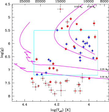
Figure 4. Effective temperature vs. surface gravity for the final sample of 57+3 low-mass WD candidates. Cyan box marks our clean ELM WD sample, the region that maximizes the overlap between the data and the ELM WD tracks (magenta lines; Istrate et al. 2016). Symbols are the same as in Figure 1.
Download figure:
Standard image High-resolution imageFigure 4 shows that our choice of −0.4 < (g − r)0 <−0.1 mag color is effective in selecting 9000 < Teff < 22,000 K objects and excluding stars at cooler temperatures. New objects (red symbols) are mostly found at both higher and lower  compared to the original ELM Survey, consistent with the expanded color selection, but nine of the new objects are found in the clean ELM region. We explore these objects further below.
Interestingly, the overall distribution of points in Figure 4 does not uniformly fill Teff and  space. The onset of hydrogen shell flashes in the WD evolutionary tracks around ∼0.2 M⊙ creates a gap in the tracks in Teff and
  space. Observed WDs largely overlap the WD evolutionary tracks in Teff and
  space, and do not uniformly fill the plot.
The joint parallax and color criteria are very efficient at finding ELM WDs: half (29) of our targets fall in the clean ELM WD region that directly overlaps the ELM WD tracks in the range  .
.
3.3. Disk and Halo Populations
Before selecting an evolutionary track for the analysis, we must first assess whether an observed target is a disk or halo object. We use three-dimensional space velocities to make this assessment. In brief, we compute space velocities using our systemic radial velocities, corrected for the gravitational redshift of the observed WD, and Gaia proper motions. We then compare the velocity of the low-mass WD with the velocity ellipsoid of the disk and halo as described in Brown et al. (2020b). The result is essentially the same as found by Brown et al. (2020b): 70% of the observed objects have motions consistent with the thick disk velocity ellipsoid and 30% have motions consistent with the halo.
3.4. White Dwarf Parameters
We then estimate WD mass and luminosity by interpolating the measured Teff and  through WD evolutionary tracks. For 34 objects with
  , we use Istrate et al. (2016) tracks with rotation and diffusion. We apply Z = 0.02 tracks to objects with disk kinematics, and Z = 0.001 tracks to objects with halo kinematics. We then estimate distances from the dereddened SDSS apparent magnitude and the absolute magnitude derived from the tracks,
  kpc.
kpc.
Figure 5 compares our dspec estimates derived from Istrate et al. (2016) tracks against the dgeo = 1/π distances measured geometrically by Gaia. We plot the 29 objects with distance ratio uncertainties better than 30%. The mean ratio is dspec/dgeo = 1.02 ± 0.04. Thus, the Istrate et al. (2016) tracks provide a remarkably accurate measure of mass and radius for ELM WDs.
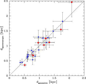
Figure 5. Spectroscopic distance estimates derived from Istrate et al. (2016) ELM WD tracks compared to geometric distances measured from Gaia eDR3. Symbols are the same as in Figure 1. Dotted line is the 1:1 ratio.
Download figure:
Standard image High-resolution imageThe most discrepant point in Figure 5 is one of the new ELM WD binaries, J2104+1712, with dspec/dgeo = 0.69 ± 0.15. J2104+1712 is a P = 5.7 hr binary. Our spectra show no evidence for a double-lined spectroscopic system or emission in the cores of the Balmer lines; however, it is possible that such effects could artificially inflate our  measurement. If the actual
  were 0.5 dex lower (the WD had a larger radius), the derived absolute magnitude would be ∼1 mag more luminous for the same temperature and bring the spectroscopic distance into agreement with the geometric distance.
For the remaining objects that do not overlap the Istrate et al. (2016) tracks, we estimate WD parameters using Althaus et al. (2013) helium-core WD tracks for objects up to  , and Tremblay et al. (2011) WD tracks for objects above
  . We note that dspec estimates for the high-gravity WDs are systematically smaller than the Gaia distances, very similar to J2104+1712, but we defer a detailed investigation. We focus our attention on the well-measured ELM WDs.
3.5. Binary Orbital Solutions
Follow-up time-series spectroscopy reveals significant 200 to 1100 km s−1 radial-velocity variability in every  target. Velocity variability in
  targets is not significant given our observational errors. For the new targets with
  , we acquire a total of 10 to 20 spectra spaced over a few different nights. This sampling is sufficient to determine binary orbital elements for 14 targets, plus another 3 targets at slightly higher
  . Only one object in the clean ELM region, J1240−0958, lacks sufficient coverage to determine its orbital parameters.
Table 2 presents the 17 binaries, and Figure 6 presents the radial velocities phased to the best-fit orbital solution. Our computational approach is to minimize χ2 for a circular orbit fit to each set of radial velocities. We estimate errors by resampling the radial velocities with their errors and refitting the orbital solution 10,000 times. We report the 15.9% and 84.1% percentiles of the parameter distributions in Table 2. Systemic velocities are corrected for gravitational redshift using the WD parameters in Table 2. One target, J0745+2104, has a significant period alias, and therefore is excluded from Figure 6.
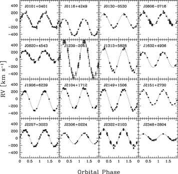
Figure 6. Radial velocities phased to the best-fit orbital period for the new ELM WD binaries. The measurements for all 17 binaries are available as data behind the figure.(The data used to create this figure are available.)
Download figure:
Standard image High-resolution imageTable 2. Binary Parameters
| Object | P | k | γ |

|

|
|---|---|---|---|---|---|
| (days) | (km s−1) | (km s−1) | (M⊙) | (yr) | |
| J0101+0401 | 0.18332 ± 0.00284 | 199.5 ± 7.1 | −11.3 ± 6.9 | >0.35 | <9.8 |
| J0116+4249 | 0.33400 ± 0.00015 | 237.8 ± 4.6 | −204.7 ± 3.1 | >0.81 | <10.1 |
| J0130−0530 | 0.63648 ± 0.00072 | 191.2 ± 5.7 | −29.3 ± 3.9 | >0.85 | <10.8 |
| J0745+2104 | 0.53964 ± 0.00511 | 132.2 ± 4.6 | 55.0 ± 3.6 | >0.46 | <10.7 |
| J0806−0716 | 0.70555 ± 0.01554 | 170.7 ± 11.2 | 26.9 ± 13.6 | >0.63 | <11.1 |
| J0820+4543 | 0.31553 ± 0.00042 | 153.1 ± 3.7 | 86.5 ± 3.1 | >0.44 | <10.1 |
| J1239−2041 | 0.01563 ± 0.00013 | 557.2 ± 10.4 | −8.9 ± 7.5 | >0.61 | <6.6 |
| J1313+5828 | 0.07395 ± 0.00018 | 321.7 ± 6.5 | −21.3 ± 4.8 | >0.56 | <8.5 |
| J1632+4936 | 0.10141 ± 0.00016 | 209.7 ± 7.2 | −16.1 ± 6.7 | >0.33 | <9.0 |
| J1906+6239 | 0.32939 ± 0.00005 | 271.2 ± 3.0 | −57.8 ± 3.2 | >1.06 | <10.0 |
| J2104+1712 | 0.23750 ± 0.00022 | 286.6 ± 6.0 | 7.6 ± 5.2 | >0.86 | <9.8 |
| J2149+1506 | 0.08541 ± 0.00016 | 290.3 ± 12.0 | −31.2 ± 4.7 | >0.51 | <8.7 |
| J2151+2730 | 0.51593 ± 0.00316 | 203.9 ± 6.7 | 31.0 ± 10.3 | >0.72 | <10.8 |
| J2257+3023 | 0.13489 ± 0.00016 | 226.3 ± 3.2 | 2.1 ± 2.8 | >0.47 | <9.1 |
| J2306+0224 | 0.28728 ± 0.00009 | 148.3 ± 5.7 | −11.5 ± 4.2 | >0.28 | <10.4 |
| J2322+2103 | 0.02220 ± 0.00025 | 248.1 ± 4.3 | 7.8 ± 3.3 | >0.19 | <7.5 |
| J2348+2804 | 0.92013 ± 0.01532 | 89.3 ± 12.2 | 30.4 ± 11.8 | >0.25 | <11.7 |
Note. J0745+2104 observations have a period alias at P = 0.343 days.
Download table as: ASCIITypeset image
3.6. Time-series Photometry of J1239−2041
J1239−2041 is the shortest-period (P = 22.5 minutes) binary in the new discoveries, and among the shortest-period detached WD binaries known. Ultracompact P < 1 hr WD binaries commonly exhibit ellipsoidal variation, reflection effects, and eclipses in their light curves, all of which constrain the inclination of the binary (e.g., Hermes et al. 2014; Burdge et al. 2020b).
We used Gemini South GMOS to acquire time-series imaging of J1239−2041 on UT 2021 June 28 as part of the program GS-2021A-DD-108. We obtained 161 back-to-back g-band exposures over a 66 minute baseline to test for photometric variability. The short time-series is sufficient to rule out the presence of eclipses (Figure 7).
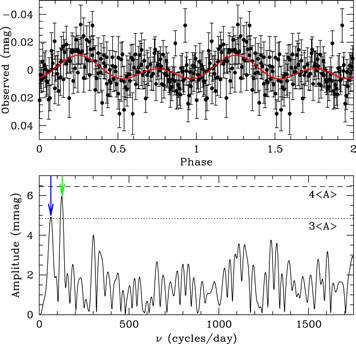
Figure 7. Gemini g-band light curve of J1239−2041 (top panel) folded at the orbital period, and repeated for clarity. The solid red line displays our best-fitting model. The bottom panel shows the Fourier transform of this light curve, and the 3〈A〉 and 4〈A〉 levels, where 〈A〉 is the average amplitude in the Fourier Transform. Blue and green arrows mark the 1× and 2× orbital frequency.
Download figure:
Standard image High-resolution imageA frequency analysis finds marginally significant photometric variability at the radial-velocity orbital period. We perform a simultaneous, nonlinear least-squares fit that includes the amplitude of the Doppler beaming ( ), ellipsoidal variations (
 ), and reflection (
 ). The best-fit model, plotted as the red line in Figure 7, has relativistic beaming = 0.45 ± 0.12%, ellipsoidal variation = 0.53 ± 0.11%, and reflection effect =
  %.
%.
We also use LCURVE to fit the mass ratio, scaled radii, effective temperatures, and velocity scale used to account for Doppler beaming and gravitational lensing. We use fixed quadratic limb-darkening values and fixed gravity-darkening values (Claret et al. 2020) based on our spectroscopic atmospheric parameters for the ELM WD and a putative 9000 K,  = 8 companion. We place Gaussian priors on the ELM WD temperature, mass, and velocity semiamplitude based on our spectroscopic and radial-velocity measurements. Our Markov Chain Monte Carlo algorithm uses 256 walkers, each performing 1000 fit iterations. We remove the first 100 of each as burn-in, leaving 230,400 iterations from which we created the final parameter distributions plotted in Figure 8. Note that LCURVE refers to the parameters of the unseen companion—the more massive star—with a subscript 1 and the ELM WD with a subscript 2.
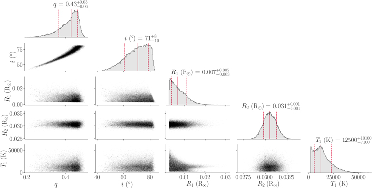
Figure 8. Corner plot showing the parameter distributions from LCURVE. The unseen companion parameters are labeled T1 and R1. The ELM WD radius, labeled R2, matches the input priors. The inclination constraint is  °.
°.
Download figure:
Standard image High-resolution imageWe derive a  M⊙ companion mass given the fitted mass ratio and our spectroscopic 0.291 ± 0.013 M⊙ ELM WD mass. As seen in Figure 8, the companion’s
  K temperature and
  R⊙ radius are poorly constrained by our short time-series observations, but the parameters are consistent with WD tracks. LCURVE returns a radius of
  R⊙ for the ELM WD in perfect agreement with input priors.
The lack of eclipses limits the inclination of J1239−2041 to i < 81°. However, the 0.53% ellipsoidal amplitude implies an approximately edge-on orientation. The LCURVE fit yields  °. We also detect Doppler beaming, and the predicted 0.38% beaming amplitude is consistent within the errors of the observed 0.45% value. A longer baseline light curve is needed to more accurately constrain J1239−2041's parameters.
4. Discussion
4.1. Observational Completeness for ELM WDs
A primary goal of this paper is to assess the observational completeness of the published ELM Survey sample. We search for probable low-mass WD candidates by expanding the original color selection region by the 3σ SDSS color uncertainties, and then applying Gaia parallax constraints to identify 57 candidates with 17 < g < 19 mag across the entire SDSS footprint in the color range −0.4 < (g − r)0 < −0.1 mag.
Follow-up observations are complete. Twenty-one candidates were previously published, and observations for the remaining 36 candidates are presented in the previous section. All but 1 of the 57 candidates are WDs. (We consider J2338+1235 a non-WD on the basis of its spectroscopic 
.44 ± 0.13. J2338+1235 has one of the poorest parallax constraints in our sample, parallax_over_error = 3.8, and its −299 ± 11 km s−1 heliocentric radial velocity suggests it is a halo star.)
In terms of target selection, the ELM Survey missed a dozen low-mass WD candidates with −0.4 < (g − r)0 < −0.1 mag in SDSS (Figure 1). Nearly all of the missing candidates are in the blue half defined by the HVS survey (Brown et al. 2012b) and are missing because they failed the selection criteria at the time of observation. The HVS Survey was executed prior to SDSS DR8 when the SDSS photometric calibration and sky coverage changed every data release. Candidates near the hot edges of the color selection in Figure 1 were particularly sensitive to the changing calibrations. J1313+5828 had (g − r)0 < −0.40 in DR7 and earlier data releases, for example, and so was not included in the original sample. Five candidates located at southern Galactic latitudes or low decl. did not appear in SDSS sky coverage until DR8. Four more candidates were actually observed by the HVS Survey, but were not included in ELM Survey follow-up because the first spectra indicated  surface gravity and the objects were not considered probable WDs.
In terms of sample completeness for ELM WDs, we estimate that the published ELM Survey was 90% complete. Our observations identify a total of 9 new ELM WDs, 10 if you count J2306+0224 just outside the clean ELM WD region in Figure 4. Only three of the new ELM WDs fall in the original color selection criteria: a 9% increase in the clean sample of ELM WDs with 17 < g < 19 mag and −0.4 < (g − r)0 < −0.1 mag. This color-selected sample should now be complete over the entire SDSS footprint.
Of course ELM WDs exist outside our original color selection criteria, as demonstrated by the broader selection used in this paper. Yet most of the candidates from the expanded color selection in Figure 1 are normal WDs. Torres et al. (2022) estimate that only 1% of all WDs are He-core objects based on the Gaia 100 pc sample. Applying a joint parallax constraint is thus important for identifying real ELM WDs in a crowded region of parameter space. It is interesting to explore how other Gaia-based catalogs of WDs and ELM WD candidates compare.
4.1.1. Comparison with Gaia WD Catalogs
Figure 9 compares the clean ELM WD sample with the Gentile Fusillo et al. (2021) Gaia eDR3 WD catalog and the Pelisoli & Vos (2019) Gaia DR2 ELM WD candidate catalog. We restrict the figure to objects within SDSS with 17 < g < 19 mag to make a one-to-one comparison.
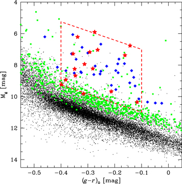
Figure 9. Comparison of our clean ELM WD sample (blue and red symbols, same as Figure 2), high-confidence WDs from the Gentile Fusillo et al. (2021) Gaia eDR3 WD catalog (black dots), and objects from the Pelisoli & Vos (2019) Gaia DR2 ELM WD candidate catalog (green squares). To make a fair comparison, we plot only those objects within SDSS with 17 < g < 19 mag.
Download figure:
Standard image High-resolution imageGentile Fusillo et al. (2021) select 1.3 million WD candidates from the Gaia eDR3 catalog from which they identify 390,000 high-confidence PWD > 0.75 sources. The 21,500 high-confidence sources with SDSS 17 < g < 19 mag are drawn as black dots in Figure 9. The majority of sources fill the locus of normal WDs.
Interestingly, the Gentile Fusillo et al. (2021) WD catalog includes 58 of our 60 objects, and two-thirds (38) are high-confidence WDs. The Gentile Fusillo et al. (2021) photometric hydrogen-atmosphere parameter estimates are not very reliable for our class of objects: on average 7 ± 16% lower in Teff and 0.4 ± 0.5 dex lower in  than our spectroscopic values. Furthermore, the 20 objects in our sample classified as low-confidence WDs are spectroscopic
  low-mass WDs. Two objects in our sample that are not listed in the Gentile Fusillo et al. (2021) catalog are the background halo star (J2338+1235) and a P = 15.28 hr ELM WD binary, J0130−0530.
Pelisoli & Vos (2019) perform a similar astrometric selection optimized for ELM WDs and identify 5762 candidates using Gaia DR2. The 703 candidates with SDSS 17 < g < 19 mag are drawn as green squares in Figure 9. The Pelisoli & Vos (2019) catalog includes half (31 of our 60) of our objects. The matches are a 50/50 mix of ELM WDs and other WDs. The other half of our objects are missing in the Pelisoli & Vos (2019) catalog, including the shortest-period ELM WD binaries. This likely reflects their parallax selection and the Gaia DR2 parallax errors.
While there is clear overlap between our ELM WD selection and existing Gaia-based catalogs, it is less clear how to compare the underlying selection criteria. The Gentile Fusillo et al. (2021) catalog is focused on normal  WDs, and so may provide a better means to exclude normal WDs (and possibly background halo stars, which should not exist in the WD catalog) from a search for ELM WDs than the other way around. Pelisoli & Vos (2019) intentionally target ELM WDs but with low efficiency. If we restrict the Pelisoli & Vos (2019) catalog to candidates with SDSS 17 < g < 19 mag and −0.4 < (g − r)0 < −0.1 mag—our ELM WD sample should be essentially complete in this magnitude and color range—then 4.5% (16 of 357) of the Pelisoli & Vos (2019) candidates are ELM WDs with
  . Figure 9 suggests that the remaining candidates are likely WDs with higher >0.3 M⊙ masses. We conclude that the combination of multipassband photometry and parallax makes for a more efficient selection of ELM WDs.
4.2. New LISA Verification Binaries
One reason ELM WDs are interesting is that they reside in ultracompact binaries. Nearly two-thirds (35 of 57) of the candidates in the current sample are detached, double degenerate binaries. Two of the newly discovered binaries have orbital periods less than 32 minutes and are potential LISA gravitational-wave sources.
J1239−2041 was first identified as a 0.29 M⊙ ELM WD by Kosakowski et al. (2020) in ELM Survey South observations. Follow-up motivated by the object’s SDSS colors and Gaia parallax reveal it to be a P = 22.514 ± 0.186 minute binary. The K = 557.2 ± 10.4 km s−1 semiamplitude requires an M2 > 0.61 M⊙ minimum mass companion at ≃ 0.25 R⊙ separation. This is a double degenerate binary, one that will merge in < 4 Myr due to loss of energy and angular momentum via gravitational-wave radiation. Located at a heliocentric distance of d = 0.89 ± 0.11 kpc, the NASA LISA Detectability Calculator 6 estimates LISA will detect J1239−2041 with a 4 yr signal-to-noise ratio (S/N) = 12.
J2322+2103 is a 0.25 M⊙ ELM WD in a  minute binary. Its K = 248.1 ± 4.3 km s−1 semiamplitude requires an M2 > 0.19 M⊙ minimum mass companion with a < 30 Myr gravitational-wave merger time. Located at a heliocentric distance of d = 1.04 ± 0.16 kpc, J2322+2103 has an estimated LISA 4 yr S/N = 3.5.
Figure 10 plots the distribution of characteristic strain versus gravitational-wave frequency, fGW = 2/P, for the current sample (solid symbols) and all other ELM Survey binaries (open symbols) compared to the LISA 4 yr sensitivity curve (Robson et al. 2019). New binaries are red; previously published binaries are blue. The overall distribution reflects the fact that these detached WD binaries look like constant frequency sources to LISA, so their S/N is proportional to  orbits in 4 yr. Burdge et al. (2020b) target similar sources with P < 1 hr variability in the Zwicky Transient Factory and have discovered even shorter period systems (Burdge et al. 2019, 2020a).
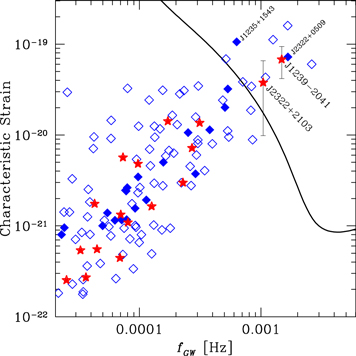
Figure 10. Characteristic strain vs. gravitational-wave frequency for the current sample (solid symbols) and all other ELM Survey binaries (open diamonds) compared to the LISA 4 yr sensitivity curve (Robson et al. 2019). As before, new binaries are red, and previously published binaries are blue.
Download figure:
Standard image High-resolution imageFour of the 35 binaries in the current sample are likely LISA sources: J1239−2041 and J2322+2103, plus J1235+1543 (Kilic et al. 2017) and J2322+0509 (Brown et al. 2020a). All four are labeled in Figure 10. Interestingly, their LISA S/N may be underestimated. Recent work shows that if the observed metallicity dependence of the stellar binary fraction is applied to WD models (Thiele et al. 2021), or if the separation distribution of observed low-mass WD binaries is applied to all classes of WDs (Korol et al. 2022), then the predicted gravitational-wave foreground may be reduced by a factor of 2 for resolved LISA sources. Regardless, ELM WD binaries are a significant source of LISA “verification binaries,” known binaries observable with both light and gravitational waves.
5. Conclusions
We use Gaia parallax and SDSS multipassband photometry to identify ELM WD candidates. A joint parallax and color selection yields 57 ELM WD candidates with 17 < g < 19 mag over the entire SDSS footprint in the color range −0.4 < (g − r)0 < −0.1 (approximately 9000 K < Teff < 22,000 K). Observations presented here complete the sample.
The joint target selection is highly efficient for finding ELM WDs: 50% of the candidates fall in the clean ELM WD region  that overlaps the ELM WD evolutionary tracks. All of the clean sample of ELM WDs are detached, double degenerate binaries with P < 1 day orbits.
The 17 binaries published here bring the ELM Survey sample to 124 WD binaries. We find that 10% of low-mass WD binaries have P < 1 hr orbits relevant to LISA. This implies that doubling the sample of low-mass WDs, for example, by surveying the southern sky with SkyMapper as we have done with SDSS in the north, should yield a dozen new multimessenger WD binaries observable with LISA.
We thank M. Alegria, B. Kunk, E. Martin, and A. Milone for their assistance with observations obtained at the MMT telescope, and Y. Beletsky for their assistance with observations obtained at the Magellan telescope. We thank the referee for constructive feedback that improved this paper. This research makes use the SAO/NASA Astrophysics Data System Bibliographic Service. This work was supported in part by the Smithsonian Institution and in part by the NSF under grant AST-1906379.
The Apache Point Observatory 3.5 m telescope is owned and operated by the Astrophysical Research Consortium.
Based on observations obtained at the Southern Astrophysical Research (SOAR) telescope, which is a joint project of the Ministério da Ciência, Tecnologia e Inovações (MCTI/LNA) do Brasil, the US National Science Foundation’s NOIRLab, the University of North Carolina at Chapel Hill (UNC), and Michigan State University (MSU).
Based on observations obtained at the international Gemini Observatory, a program of NSF’s NOIRLab, which is managed by the Association of Universities for Research in Astronomy (AURA) under a cooperative agreement with the National Science Foundation. on behalf of the Gemini Observatory partnership: the National Science Foundation (United States), National Research Council (Canada), Agencia Nacional de Investigación y Desarrollo (Chile), Ministerio de Ciencia, Tecnología e Innovación (Argentina), Ministério da Ciência, Tecnologia, Inovações e Comunicações (Brazil), and Korea Astronomy and Space Science Institute (Republic of Korea).
Facilities MMT (Blue Channel spectrograph), Magellan:Clay (MagE spectrograph), SOAR (Goodman spectrograph), APO 3.5 m (DIS spectrograph), Gemini:South (GMOS spectrograph).
Software: IRAF (Tody 1986, 1993), RVSAO (Kurtz & Mink 1998), LCURVE (Copperwheat et al. 2010).
Footnotes
- 5
Gentile Fusillo et al. (2021) high Galactic latitude data quality cut used: (astrometric_sigma5D_max < 1.5 OR (ruwe ≤ 1.1 AND ipd_gof_harmonic_amplitude < 1)) AND (phot_bp_n_obs > 2 AND phot_rp_n_obs > 2) AND (∣phot_br_rp_excess_factor_corrected∣ < 0.6) AND (astrometric_excess_noise_sig < 2 OR (astrometric_excess_noise_sig ≥ 2 AND astrometric_excess_noise < 1.5)).
- 6