Abstract
As the disk formation mechanism(s) in Be stars is(are) as yet unknown, we investigate the role of rapidly rotating radiation-driven winds in this process. We implemented the effects of high stellar rotation on m-CAK models accounting for the shape of the star, the oblate finite disk correction factor, and gravity darkening. For a fast rotating star, we obtain a two-component wind model, i.e., a fast, thin wind in the polar latitudes and an Ω-slow, dense wind in the equatorial regions. We use the equatorial mass densities to explore Hα emission profiles for the following scenarios: (1) a spherically symmetric star, (2) an oblate star with constant temperature, and (3) an oblate star with gravity darkening. One result of this work is that we have developed a novel method for solving the gravity-darkened, oblate m-CAK equation of motion. Furthermore, from our modeling we find that (a) the oblate finite disk correction factor, for the scenario considering the gravity darkening, can vary by at least a factor of two between the equatorial and polar directions, influencing the velocity profile and mass-loss rate accordingly, (b) the Hα profiles predicted by our model are in agreement with those predicted by a standard power-law model for following values of the line-force parameters:  , and
, and  , and (c) the contribution of the fast wind component to the Hα emission line profile is negligible; therefore, the line profiles arise mainly from the equatorial disks of Be stars.
1. Introduction
A classical Be star has historically been defined as “a non-supergiant” B star whose spectrum has, or had at some time, one or more Balmer lines in emission (Collins 1987). Currently, there is consensus that Be stars are very rapidly rotating and non-radially pulsating B stars (of luminosity class V–III), forming a decretion disk of outwardly flowing gas rotating in a Keplerian fashion (Rivinius et al. 2013). It is generally accepted that Be star disks are geometrically thin and produced from material ejected from the central star.
An observational feature of these stars is the presence of emission lines from the optical to the near-IR wavelength regions of the spectrum. These lines can be formed in a region very close to the star (helium and doubly ionized metal lines), in a large part of the disk (hydrogen lines), or relatively far from the star (singly ionized metal lines, Rivinius et al. 2013). One of the predominant emission lines is the  line, and because it forms in a large region of the disk, it is often modeled to obtain average disk properties. Currently, Be star disks are frequently modeled by assuming a simple power-law density distribution in the radial direction (
 ) following the works of Waters (1986), Cote & Waters (1987), Waters et al. (1987), Jones et al. (2008), and Silaj et al. (2014b). Typically, the values for the radial power-law index n are found to be in the range 2.0–3.5, based on fits to Hα or the IR continuum (Waters 1986; Silaj et al. 2014b).
Another observational feature of Be stars is the structure of their stellar winds. Observations of broad shortward shifted UV lines of superionized elements (C iv, Si iv, and N v) demonstrate the presence of high-velocity stellar winds, even for later Be spectral types, whereas in normal B stars they are typically observed only in the early spectral types (Prinja 1989). Furthermore, these winds also suggest a trend of increasing  (ratio of terminal velocity to escape velocity) as a function of
  (ratio of projected rotational velocity to critical rotation speed), which is in contradiction with the radiation-driven wind theory or m-CAK theory (Friend & Abbott 1986; Pauldrach et al. 1986), based on the pioneering CAK theory of Castor et al. (1975), who predict a decrease in the terminal velocity as a function of rotational velocity (Prinja 1989). Interferometric observations have revealed some circumstellar envelopes with large-scale asymmetries along the polar directions that suggest an enhanced polar wind (Kervella & Domiciano de Souza 2006; Meilland et al. 2007). Polar winds from Be and normal B stars can properly be described by the current radiation-driven wind theory for massive stars (Rivinius et al. 2013). In contrast to this, at the equator, Be stars present a much slower and denser mass flux, which is not in agreement with the standard radiation-driven wind theory.
The precise mechanism to explain the formation of Be star disks is still under debate, and many attempts to link the radiation-driven wind theory to these disks have been made. One such example is the wind-compressed disk (WCD) model proposed by Bjorkman & Cassinelli (1993). This model suggested that the wind from both hemispheres of a rapidly rotating star is deflected toward the equatorial plane, producing an outflowing equatorial disk. However, Owocki et al. (1996) investigated the effects of non-radial line forces on the formation of a WCD, and their results showed that these forces (enhanced by the gravity darkening effect) may lead to an inhibition of the outflowing equatorial disk. Later, Krtička et al. (2011) examined the mechanisms of mass and angular momentum loss via an equatorial decretion disk associated with near-critical rotation. The authors emphasized the role of viscous coupling in outward angular momentum transport in the decretion disk and radiative ablation of the inner disk from the bright central star. In this context, it has been shown that radiation-driven disk-ablation models may lead to the destruction of an optically thin Be star disk on a dynamical timescale of the order of months to years (Kee et al. 2016), without invoking anomalously strong viscous diffusion.
Viscous disk models with radiation-driven ablation are currently based on a non-rotating m-CAK wind solution that assumes a power-law distribution in line strength. It is then important to stress that when the finite disk approximation for the line acceleration (m-CAK theory, Friend & Abbott 1986; Pauldrach et al. 1986) is combined with the term of the centrifugal force on a rapidly rotating star (i.e., for  of the critical rate, with
  ), they cause the termination of the m-CAK wind solution (fast solution) in the equatorial plane, and a new solution—the Ω-slow solution—is established (Curé 2004).
The Ω-slow solution results in higher mass-loss rates and lower terminal velocities than those from a conventional fast wind solution, so it could provide proper physical conditions to form a dense disk in Keplerian rotation via angular momentum transfer.
Our model is then based on the assumption that, as main-sequence B stars evolve, with moderately rapid initial rotation and mass loss, they can bring angular momentum to the surface and spin up even to critical rotation (Ekström et al. 2008). Under this condition, stars rotating near the critical rotation speed may develop a latitude-dependent wind density structure and a dense decretion disk via transfer of angular momentum. We will assume that the governing processes of a Be star wind at high latitudes are the same as in the m-CAK wind (fast solution).
At equatorial latitudes, the rotation term in the equation of motion (EoM) will increase the mass-loss rate and decrease the terminal velocity. However, as the centrifugal term ( ) increases with latitude, because
  has larger values than
  of the critical speed, the fast solution no longer exists and the Ω-slow wind solution arises. This abrupt change in the wind regime naturally produces a two-component wind.
It is worthwhile investigating whether the resulting density structure injected via the Ω-slow solution for a fast rotating star is able to reproduce the Hα emission line observed in Be stars.
To test this hypothesis, Silaj et al. (2014a) constructed a set of models for a spherical star using only density distributions coming from the Ω-slow solution and computed the Hα line using the code Bedisk (Sigut & Jones 2007). Then they compared the resulting Hα line with synthetic line profiles computed with the ad hoc power-law model described above (see, e.g., Silaj et al. 2014b). In these models, line-force parameters were taken as free parameters. These authors found that the density distribution produced by the Ω-slow solution can explain the structure of a Be star disk when (unphysically) high values for the line-force parameter k are assumed (k = 4.0, 5.0, and even ∼9.0), in contrast to the typical k values self-consistently calculated ( ) for the fast solutions (see, e.g., Abbott 1982; Pauldrach et al. 1986). In this work, we extend the study done by Silaj et al. (2014a) using broader combinations of line-force parameters, and we discuss the effects of the star’s oblate geometry and gravity darkening. Therefore, we will consider the following scenarios: (a) a spherically symmetric central star with constant temperature; (b) an oblate central star with constant temperature and (c) an oblate central star with gravity darkening. In this framework, we also show that the contribution to the line emission coming from other latitudes above and below the equator, where the m-CAK solution governs the outflowing wind, can be neglected.
The paper is organized as follows: Section 2 presents our model approximations and describes the theory for the radiation-driven stellar winds, deriving the equations that account for the oblateness of the star, the oblate finite disk correction factor, and the gravity darkening effect. In addition, we present an overview of an ad hoc power-law model usually used to describe the disk density structure of Be stars. In Section 3, we build, using the hydrodynamic code Hydwind, a grid of models with different values of the line-force parameters, and the equatorial density structures calculated for this grid are used as input in the Bedisk code to obtain a grid of Hα line profiles. This Hα line grid is compared with the synthetic line profiles computed from the ad hoc disk density scenario that follows a power-law distribution. Section 4 summarizes the results of the hydrodynamic models and the emergent line profiles predicted from the grid of equatorial mass density. In addition, we show that the contribution of the fast wind component to the emergent emission Hα line profile is negligible. Finally, we discuss future perspectives.
2. Hydrodynamic Model
2.1. Model Approximations
Throughout this work we adopt the following approximations to describe the wind from a massive star with a large rotation rate.
- 1.In this two-component stationary and isothermal wind model, we neglect the effects of viscosity, heat conduction, and magnetic fields. At the polar regions, the wind is described by the fast wind solution from the standard m-CAK model, while at the equator, due to the high rotational speed, the outflowing disk-like wind is described by the Ω-slow solution.
- 2.The hydrodynamic wind equations are solved in the 1D m-CAK model, only for polar and equatorial directions. The wind regime for other latitudes needs to be calculated using a 2D model that takes into account all non-radial forces (see, e.g., Bjorkman & Cassinelli 1993; Cranmer & Owocki 1995; Petrenz & Puls 2000), and this is beyond the scope of this work.
- 3.Line-force parameters for the fast solutions correspond to the calculated values (see, e.g., Lamers & Cassinelli 1999 and references therein). As the line-force parameters for the Ω-slow solution have so far no self-consistent calculations, we adopt ranges:
 and (see Kudritzki 2002), while k is varied within a wider range.
 - 4.The m-CAK model with rotation assumes conservation of angular momentum.


In the following sections, we incorporate the effect of the distortion of the star’s shape caused by its high rotational speed and the gravity darkening effect into the radiation-driven wind theory.
2.2. Radiation-driven Wind Equations
The 1D m-CAK hydrodynamic equations for rotating radiation-driven winds, namely conservation of mass and of radial momentum, considering spherical symmetry, and neglecting the gravity darkening effect and non-radial velocities, are

and
where r is the radial coordinate, Fm is the local mass-loss rate, v is the fluid radial velocity, dv/dr is the velocity gradient, and gline is the radiative acceleration as a function of ρ and  , the mass density and electron number density, respectively.
  , the Eddington factor, is the Thomson electron scattering force divided by the gravitational force. The gas pressure, p, is given in terms of the sound speed, a, for an ideal gas as
  . The variables
  , and ρ are functions of position and co-latitude angle. In addition, the variables a and
  become functions of co-latitude when gravity darkening is taken into account. The rotational speed
  is calculated assuming conservation of angular momentum, where
  is the star’s surface rotational speed at co-latitude θ, expressed by

with  being the stellar rotational speed at the equator.
The CAK theory assumes that the radiation emerges directly from the star (as a point source) and multiple scatterings in different lines are not taken into account. A later improvement to this theory (m-CAK) considers the radiation emanating from a stellar disk, and therefore we adopt the m-CAK standard parameterization for the line-force term, following the descriptions of Abbott (1982), Friend & Abbott (1986), and Pauldrach et al. (1986), namely
where the coefficient (eigenvalue) C is given by
here Fm is calculated once the eigenvalue is obtained. In these equations, W(r) is the dilution factor,  is given in units of
  is the mean thermal velocity of the protons, and
  is expressed as

where  is the electron scattering opacity per unit mass.
The line-force parameters (Abbott 1982; Puls et al. 2000) are given by α (the ratio between the line-force from optically thick lines and the total line force), k (which is related to the number of lines effectively contributing to the driving of the wind), and δ (which accounts for changes in the ionization throughout the wind).
The finite disk correction factor,  , for a spherical star, is defined as
where
All other variables have their standard meaning. (For detailed derivations and definitions of variables, constants, and functions, see, e.g., Curé 2004).
In addition, we can define the normalised stellar angular velocity as

where  is the critical rotational speed for a spherical star, defined, e.g., by Maeder & Meynet (2000) as
where  considers the mean opacity of the total flux, κ, instead of the electron scattering opacity per unit mass used in the theory of radiatively driven winds given in Equation (6). Because of the difficulty of knowing the exact value of κ, our values for
  are calculated assuming
  . This approximation represents a minor underestimation of the value of Ω, since in our models both
  and
and  are
are  .
.
2.3. Oblateness and Gravity Darkening Effects
When we take high rotation into account, the star becomes oblate and its shape becomes roughly similar to a rotating ellipsoid. The von Zeipel theorem states that the radiative flux  at some co-latitude in a rotating star is proportional to the local effective gravity,
  (von Zeipel 1924). This oblateness changes the local effective gravity,
  (sum of the gravitational and centrifugal accelerations), and hence the local temperature at the stellar surface (von Zeipel 1924, for shellular rotation see Maeder 1999). For this reason, when we consider both effects, it is convenient to redefine some parameters as a function of co-latitude θ and rotational speed.
Thus, the star’s local rotational speed is given by

and the normalized stellar angular velocity is expressed as
where, in a Roche model,  is the maximum equatorial radius when a star is rotating at the critical velocity, i.e.,
  (see, e.g., Puls et al. 2008; Müller & Vink 2014).
  is the polar radius, and as a first approximation it is assumed to be independent of the rotational velocity.6
Then, the critical rotational velocity for a uniform radiation field, where the effect of gravity darkening is omitted, is expressed as
is the polar radius, and as a first approximation it is assumed to be independent of the rotational velocity.6
Then, the critical rotational velocity for a uniform radiation field, where the effect of gravity darkening is omitted, is expressed as
It is important to note that when gravity darkening is considered,  requires special attention. Puls et al. (2008) state: “After some controversial discussions arising from the suggestion of an Ω limit by Langer (1997, 1998) which has been criticized by Glatzel (1998) (because of disregarding gravity darkening), Maeder & Meynet (2000) performed a detailed study on the issue.” Maeder & Meynet (2000) state that some authors write the critical rotational velocity as in Equation (10), but they emphasize that this relation is true only if it is assumed that the brightness of the rotating star is uniform over its surface. This is in contradiction with the von Zeipel theorem, which predicts a decrease in the effect of radiation pressure at the equator. Surprisingly for Maeder & Meynet (2000), some authors use this relation simultaneously with the von Zeipel theorem. Maeder & Meynet (2000) establish that the critical rotational velocity is reached when the total gravity
  , i.e.,

where  is the local Eddington factor. Their study finds that for moderate values of
  (which is our case) the critical speed can be calculated, independently from
  , from the condition
  , in agreement with Glatzel (1998), as
The stellar radius can be approximated as a function of co-latitude and rotational speed as

(Cranmer & Owocki 1995; Petrenz & Puls 1996; Müller & Vink 2014).
The local effective gravity at a given co-latitude, directed inward along the local surface normal, is given by the negative gradient of the effective potential

(Cranmer & Owocki 1995; Maeder & Meynet 2000). Thus, the two-components of the local effective gravity in spherical coordinates are

and

Then, the absolute value of the local effective gravity is

or
On the other hand, to derive the dependence of  on the co-latitude at the surface of the star, we follow the work of Espinosa Lara & Rieutord (2011), who assume that the radiative flux in the envelope of a rotating star can be expressed, following von Zeipel (1924), as

where  is a function of the position to be determined and satisfies the condition

and η is a constant that scales the function f and can be rewritten in a dimensionless form as

Then for the Roche model,  , an expression for the local effective temperature can be derived (see Espinosa Lara & Rieutord 2011):
and furthermore  . This last equation possesses singularities at the poles and the equator of the star. At these points, the local effective temperature is respectively given by
and
Since the effective gravity, and therefore the flux, varies over the surface of the rotating star, we still need to determine the local value of  for a barotropic case of a nonspherical star that can be defined in terms of the reduced mass, M★, as follows:

with
where  is the internal average density (Maeder 1999; Maeder & Meynet 2000). It is important to note that the value of
  is independent of latitude.7
In order to account for the oblateness of a gravity-darkened star, we need to calculate the corresponding oblate finite disk correction factor  at a given co-latitude,
The reader is referred to Figure 2 and Section 4.3 from Pelupessy et al. (2000) for the definition of the various angles.8
Here we neglect the continuum correction factor since it is not important for low-luminosity stars because  itself is small.
2.4. Solving the Hydrodynamic Wind Equations
In order to solve the 1D hydrodynamic radiation-driven wind equations, Curé (2004) introduced the following change of variables:  , and
, and  , with
  , where a is the isothermal sound speed. Based on this auxiliary set of variables, we can write an approximate EoM for an oblate gravity-darkened star valid for
  , where
  is evaluated with
  instead of κ,
where
To solve this nonlinear differential equation we adopt  and define now A and
  in terms of
  :
:

and
with
and
where  is the helium abundance relative to hydrogen,
  is the number of free electrons provided by helium,
  is the atomic mass number of helium, and
  is the mass of the proton.
A more general expression for the EoM valid for larger values of  can be found in Appendix A. In Appendix B we show the calculation of
  .
.
In order to find a physical, continuous solution of w, which starts at the stellar surface and reaches infinity, it is necessary to require the solution to pass through a critical (singular) point. Its location is obtained from the singularity condition,

together with a lower boundary condition (at the stellar surface) by setting the surface mass density to a specific value,

At the critical point a regularity condition must be imposed, namely,

where the last term  , due to the singularity condition (Equation (37)).
Depending on the value of Ω, the solution of Equation (31) leads to either fast or Ω-slow wind solutions. Notice that for high rotational velocities, the standard (or fast) solution ceases to exist (Curé 2004). In both cases, we use the stationary hydrodynamic Hydwind code (Curé 2004) modified to take into account the effects of oblateness and gravity darkening.
2.5. Calculation of the Gravity-darkened and Oblate Finite Disk Correction Factor
To solve the m-CAK EoM accounting for the gravity darkening and the oblate distortion of the star that is caused by its rapid rotation, we implemented the method described by Araya et al. (2011), who introduced the  factor and its calculation. In view of the behavior of the
  factor, it is possible to obtain an approximate expression via a sixth-order polynomial interpolation in the inverse radial variable u, i.e.,

With this structure, the different topological solutions of the m-CAK model, found by Curé (2004), are maintained by the  term, but modified by the incorporation of this Q(u) polynomial. This approximation (Equation (40)) allows the nonlinear m-CAK EoM to be solved in a straightforward way, instead of calculating the complicated integral of
  (Equation (30)), which would be computationally expensive and numerically unstable.
In this work we solve the m-CAK EoM for the polar and equatorial directions (see Section 4), but in the calculation the latitude dependence of the oblate finite disk correction factor and the gravity darkening are taken into account.
A finite-difference iterative numerical method, described in Curé (2004), is used to solve this nonlinear differential equation. This numerical approach needs to start from an initial trial velocity profile in order to iterate until convergence. Therefore, our iterative strategy is as follows:
- 1.A initial β-law for the velocity profile is used for v(u) and w(u).
- 2. and are calculated from w(u).
- 3.Q(u) coefficients are calculated by fitting as function of u.
- 4.The EoM is solved with our approximate, obtaining a new velocity profile w(u).
- 5.Steps 2 to 4 are repeated until convergence is reached.


A comparison between Q(u) and the ratio  is shown in Figure 1 for the equatorial (upper panel) and polar (lower panel) regions. Both functions were calculated for
  considering the oblate finite disk correction factor and gravity darkening. We find discrepancies of about 2% after four iterations. The oblate correction factors are depicted in Figure 2: the solid line is calculated by solving Equation (30) numerically, and the dashed line is obtained from our approximation. The excellent agreement between the approximated and the numeric
  factors, at the pole and equator, demonstrates the robustness of this method. It is important to emphasize the intensity variation that results from the integration of the
  factor with co-latitude when gravity darkening effects are taken into account. In order to understand and compare the behavior of the scenario with gravity darkening in Figure 3 we also show
  without considering the gravity darkening. From the plots we can observe the large impact of
  on the polar direction, where the intensity between the models with and without gravity darkening follows a similar behavior. Finally, in order to test our calculation for
  , we show in Figure 4 a comparison between
  with gravity darkening and
  , both for a low value of Ω (
 ) at the equator and the pole. At this rotational speed, the star remains almost spherical and the temperature essentially constant, confirming that the two correction factors are similar.
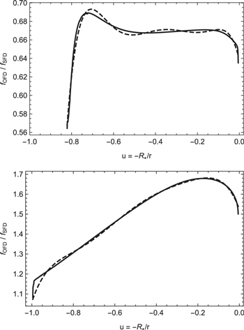
Figure 1. Comparison of the ratio  (solid line) with the polynomial interpolation Q(u) (dashed line) at the equator (upper panel) and the pole (lower panel). Both expressions have been computed for a wind model solution with
  considering oblateness and gravity darkening effects. Note that in the upper panel the function does not start at
  , due to the oblateness of the star. R* corresponds to the polar radius of an oblate star.
Download figure:
Standard image High-resolution image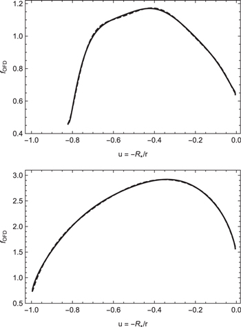
Figure 2. Comparison of the oblate correction factor calculated from Equation (30) (solid line) with the approximate oblate correction factors obtained from our iterative method (dashed line) at the equator (upper panel) and the pole (lower panel) for a model with  , including gravity darkening.
Download figure:
Standard image High-resolution image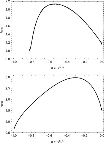
Figure 3. Similar to Figure 2, but the oblate correction factor (obtained from Equation (30)) is calculated at the equator (upper panel) and the pole (lower panel) without considering gravity darkening.
Download figure:
Standard image High-resolution image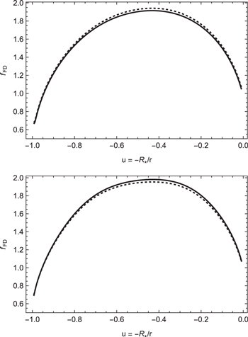
Figure 4. Comparison between  with gravity darkening (solid line) and
  (dotted line) calculated at the equator (upper panel) and the pole (lower panel) for a rotating star at
  . The correction factors in the two panels are very similar.
Download figure:
Standard image High-resolution image3. Methodology for Modeling a Be Star Disk
3.1. Ad hoc Density Model
In this section we present a short summary of the traditional method to model a thin rotating circumstellar disk.
An ad hoc disk density model is generally adopted to describe the stratification of the mass density in the equatorial plane of a thin disk. This density distribution, originally developed by Waters et al. (1987) for the interpretation of IR observations of Be stars, is assumed to follow a power-law distribution defined by
where  is the equatorial density of the disk at the stellar surface, n is the adopted power-law index, and H is the scale height in the z-direction expressed as
where  is defined as

where  is the mean molecular weight of the gas and T0 is an assumed isothermal temperature used for setting the scale height prior to the calculation of the self-consistent temperature distribution in the disk.
This simple prescription of a density distribution with power-law fall-off in the radial direction and in approximate hydrostatic equilibrium in the z-direction has been used extensively in the literature, so it provides a good basis for comparison with other works (see, for example, Sigut et al. 2015; Patel et al. 2016; Arcos et al. 2017).
Under the assumption of radiative equilibrium, the level populations and ionization state of the gas are calculated throughout the disk with the stellar radiation included using a Kurucz model atmosphere (Kurucz 1993). In addition, the code solves the transfer equation along a set of rays parallel to the star’s rotation axis. Then, by projecting the line flux at different angles, it is possible to calculate a synthetic line profile as seen by an external observer from a given line of sight (see Sigut & Jones 2007 for details).
3.2. Hydrodynamic Density Model
As mentioned in Section 1, the spirit of this work is to extend the study developed by Silaj et al. (2014a), who modeled a Be star considering: (i) a spherical star with constant effective temperature, and (ii) a thin disk using density distributions provided by the Ω-slow solution at the equatorial plane. They used these density distributions as input in the Bedisk code to obtain synthetic Hα line profiles.
In this work we also include the effect of the stellar rotation on the shape of the star and gravitational darkening. The resulting radial density structure of the equatorial plane, obtained from the Hydwind code, is then used as input in the Bedisk code, to calculate the vertical densities (z-direction) and temperature distributions, and then the synthetic Hα line profiles. It is important to note that the contribution from the outflowing wind at non-equatorial latitudes (fast wind solution) to the Hα emission line profile is negligible, as explained in Section 5. Thus, the Hα emission line-forming region is primarily in or near the equatorial plane.
Here, it is worth mentioning that the radial density distribution obtained with the Hydwind code is calculated assuming conservation of angular momentum. However, based on observations, it is commonly accepted that the disks of Be stars are in Keplerian orbits, and therefore, in order to satisfy this observational feature, Bedisk computes the synthetic line profile with a Keplerian rotational distribution to obtain the emission line as a function of wavelength.
4. Results
In this work we solve an improved rotating radiation-driven wind model considering three different scenarios: (1) a spherically symmetric star with constant temperature, (2) an intermediate scenario that considers an oblate star but neglects gravity darkening effects, and (3) an oblate star with gravity darkening. For each scenario we calculate the density stratification from the EoM (Ω-slow solution, for  ) in the equatorial plane and obtain the corresponding synthetic Hα line profiles from Bedisk. To investigate the results of these three scenarios, we first build a grid of hydrodynamic models.
4.1. Grid of Hydrodynamic Models
We adopt the same stellar parameters as Silaj et al. (2014a):  = 25,000 K,
  ,
,  , which correspond to a B1V type star. Furthermore, we set
  (see Equation (38)) as a lower boundary condition for the Hydwind code. This boundary condition ensures that the initial surface velocity is less than the sound speed.
To represent a fast rotating star we use the following Ω values:  , and 0.99. Then, the corresponding values for
  are 0.026, 0.028, 0.030, and 0.032, which are slightly larger than
  .
.
To date, there are no self-consistent values for the line-force parameters for the Ω-slow solution. Therefore, we adopt values for α and δ that are within the typical ranges calculated previously with both LTE (Abbott 1982) and non-LTE (Pauldrach et al. 1986) approximations, and we let the line-force parameter k vary in a wider range. The line-force parameters used to construct the grid of models are shown in Table 1. A total of 768 models were calculated initially with Hydwind for each of our three scenarios.
Table 1. Combinations of the Line-force Parameters for the Grid of Models
| Parameter | Values | |||||||
|---|---|---|---|---|---|---|---|---|
| α | 0.50 | 0.55 | 0.58 | 0.60 | ||||
| δ | 0.07 | 0.10 | 0.12 | 0.15 | 0.17 | 0.20 | ||
| k | 0.50 | 0.80 | 1.00 | 1.50 | 2.00 | 3.00 | 4.00 | 5.00 |
Download table as: ASCIITypeset image
Table 2 shows the stellar parameters as functions of the rotational speed for the polar and equatorial directions for all three scenarios. The values for the equatorial region are taken directly from Table 2 for our calculations for the three different scenarios. Rotational velocities are obtained from the values of Ω and  , and according to Equations (10), (13), and (15) we derive
  , and
, and  for the spherical, oblate, and oblate plus gravity darkening scenarios, respectively.
Table 2. Stellar Parameters used in Our Calculations for the Three Different Scenarios
| Ω |

|

|

|

|
Scenario |
|---|---|---|---|---|---|

|
(K) | (K) |

|
||
| 0.80 | 5.30 | 25,000 | 25,000 | 497.5 | Spherical |
| 6.05 | 25,000 | 25,000 | 308.9 | Oblate | |
| 6.05 | 22,770 | 25,802 | 312.2 | Oblate + gravity darkening | |
| 0.90 | 5.30 | 25,000 | 25,000 | 559.6 | Spherical |
| 6.44 | 25,000 | 25,000 | 370.2 | Oblate | |
| 6.44 | 21,635 | 26,020 | 374.3 | Oblate + gravity darkening | |
| 0.95 | 5.30 | 25,000 | 25,000 | 590.7 | Spherical |
| 6.79 | 25,000 | 25,000 | 411.9 | Oblate | |
| 6.79 | 20,617 | 26,139 | 416.4 | Oblate + gravity darkening | |
| 0.99 | 5.30 | 25,000 | 25,000 | 615.5 | Spherical |
| 7.37 | 25,000 | 25,000 | 465.6 | Oblate | |
| 7.37 | 18,698 | 26,240 | 470.7 | Oblate + gravity darkening | |
Download table as: ASCIITypeset image
It is worth noting that the Hydwind code can only obtain hydrodynamic solutions for some combinations of the parameters of our grid, because not all combinations have physical stationary solutions (Venero et al. 2016).
4.2. Density Distributions
Figure 5 shows the density distribution (upper panel) and velocity profiles (lower panel) at the equatorial plane for hydrodynamic models with  for our three scenarios. These models show similar terminal velocities,
  , and
, and  , respectively. Although the models presented in Figure 5 have the same set of line-force parameters, their mass-loss rates are different, namely
  , and
, and  yr−1. Both oblate models show very similar velocity profiles, but the mass-loss rate from scenario 3 is about half the value of scenario 2. This is due to the decrease in effective temperature with latitude that mainly affects the calculation of the
  factor and the radiative flux coming from the star. The difference is seen in the density distribution. Notice that in the oblate scenarios, the stellar surface in the u coordinate starts at
  due to the fact that the equatorial radius is larger than the polar one.
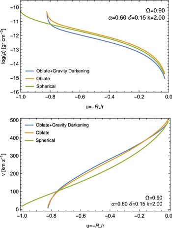
Figure 5. Mass density distributions (upper panel) and velocity profiles (lower panel) in the equatorial direction computed for rotating radiation-driven winds with  for the three scenarios as a function of the inverse radial coordinate u.
Download figure:
Standard image High-resolution imageFigure 6 compares some equatorial mass density distributions from our grid with the ad hoc mass density structure (solid black line). This ad hoc density model (Equation (41)) is calculated with  and n = 3.5 as in Silaj et al. (2014a). The mass density shows almost the same characteristic behavior for all the hydrodynamic cases. Near the surface of the star, the hydrodynamic mass density structures fall faster than the ad hoc model up to 5–8 stellar radii, and the density from the ad hoc model decays faster at greater distances.
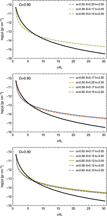
Figure 6. Mass density distributions as a function of  for the equatorial direction computed for rotating radiation-driven winds with
  and different sets of line-force parameters. The equatorial mass density distributions are compared with the ad hoc mass density structure (solid black line). These models correspond to the best-fit line profile to the ad hoc model, using the finite disk correction factor for: (i) a spherically symmetric star (top panel), (ii) an oblate star (middle panel), and (iii) an oblate star with gravity darkening (bottom panel).
Download figure:
Standard image High-resolution image4.3. Synthetic Hα Line Profiles
All mass density distributions resulting from our computations for the different scenarios were used to compute a grid of Hα line profiles with the Bedisk code.
Figure 7 shows the resulting Hα line profiles from the different mass density distributions shown in Figure 5. Since the Hα emission line is very sensitive to the mass density distribution ( ), higher densities correspond to stronger emission. As a consequence, the scenario including the gravity darkening effect has the lowest intensity in the emission line profile, because it has a lower mass-loss rate.
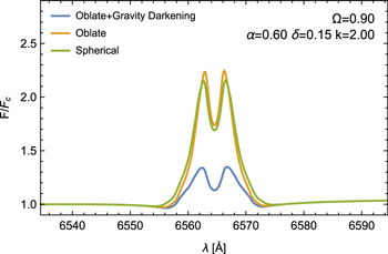
Figure 7. Comparison of Hα line profiles obtained from the Bedisk code using the density distributions shown in Figure 5. The intensities of the line profiles for the three scenarios differ because of the different mass-loss rates.
Download figure:
Standard image High-resolution imageTo select Hα profiles from our grid that best fit the profile obtained from the ad hoc density model, we define the following selection criteria: (a) our computed line profile is considered similar to the ad hoc synthetic Hα profile when the discrepancy between the maximum intensities of the line emission of the two models is lower than 15%, and (b) we adopt the smallest value of the k parameter to ensure that the k values remain physically reasonable.
Figure 8 shows the ad hoc Hα line profile compared with two profiles that are not selected by these criteria.
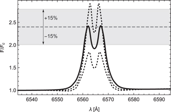
Figure 8. Comparison of the ad hoc Hα line profile (solid line) with two models (dotted lines) that lie outside our criteria (shadowed region), i.e., a discrepancy of ±15% between the maximum intensity of the ad hoc line profile (horizontal dashed line) and the maximum intensity of the profile from a calculated model.
Download figure:
Standard image High-resolution imageTable 3 summarizes the model parameters of the best fitting synthetic Hα profiles. Our results for each scenario are as follows.
Table 3.
Wind and Line-force Parameters for  , and 0.99, Showing Synthetic Hα Profiles Similar to the ad hoc Profile
| Spherical Shape | Oblate Shape | Oblate Shape + Gravity Darkening | |||||||
|---|---|---|---|---|---|---|---|---|---|
| Ω | α | δ | k |

|

|

|

|

|

|

|

|

|

|

|

|
||||
| 0.80 | 0.50 | 0.17 | 3.00 | 2.04 | 421.22 | ⋯ | ⋯ | ⋯ | ⋯ |
| 0.55 | 0.12 | 3.00 | 2.44 | 494.07 | ⋯ | ⋯ | ⋯ | ⋯ | |
| 0.55 | 0.17 | 3.00 | ⋯ | ⋯ | ⋯ | ⋯ | 3.17 | 496.51 | |
| 0.58 | 0.15 | 3.00 | ⋯ | ⋯ | ⋯ | ⋯ | 3.80 | 534.54 | |
| 0.58 | 0.20 | 2.00 | ⋯ | ⋯ | 3.69 | 526.29 | ⋯ | ⋯ | |
| 0.60 | 0.17 | 2.00 | ⋯ | ⋯ | 3.49 | 558.34 | ⋯ | ⋯ | |
| 0.90 | 0.55 | 0.17 | 3.00 | ⋯ | ⋯ | ⋯ | ⋯ | 2.61 | 438.60 |
| 0.55 | 0.20 | 2.00 | 1.95 | 419.93 | 3.10 | 443.01 | ⋯ | ⋯ | |
| 0.58 | 0.12 | 3.00 | ⋯ | ⋯ | ⋯ | ⋯ | 2.53 | 482.20 | |
| 0.58 | 0.15 | 3.00 | ⋯ | ⋯ | ⋯ | ⋯ | 3.20 | 471.83 | |
| 0.58 | 0.17 | 2.00 | 2.19 | 462.54 | 3.31 | 479.51 | ⋯ | ⋯ | |
| 0.60 | 0.10 | 3.00 | ⋯ | ⋯ | ⋯ | ⋯ | 2.76 | 507.16 | |
| 0.60 | 0.12 | 3.00 | ⋯ | ⋯ | ⋯ | ⋯ | 3.18 | 500.36 | |
| 0.60 | 0.15 | 2.00 | 2.36 | 492.80 | 3.46 | 504.56 | ⋯ | ⋯ | |
| 0.60 | 0.17 | 2.00 | ⋯ | ⋯ | 4.17 | 498.29 | ⋯ | ⋯ | |
| 0.95 | 0.55 | 0.17 | 2.00 | ⋯ | ⋯ | 2.60 | 419.66 | ⋯ | ⋯ |
| 0.55 | 0.20 | 2.00 | 2.02 | 399.08 | ⋯ | ⋯ | ⋯ | ⋯ | |
| 0.55 | 0.20 | 3.00 | ⋯ | ⋯ | ⋯ | ⋯ | 2.58 | 401.07 | |
| 0.58 | 0.15 | 2.00 | 1.88 | 447.03 | 3.11 | 450.64 | ⋯ | ⋯ | |
| 0.58 | 0.15 | 3.00 | ⋯ | ⋯ | ⋯ | ⋯ | 2.49 | 442.28 | |
| 0.58 | 0.17 | 2.00 | 2.25 | 439.93 | 3.78 | 445.10 | ⋯ | ⋯ | |
| 0.58 | 0.17 | 3.00 | ⋯ | ⋯ | ⋯ | ⋯ | 2.93 | 435.55 | |
| 0.60 | 0.12 | 3.00 | ⋯ | ⋯ | ⋯ | ⋯ | 2.55 | 469.50 | |
| 0.60 | 0.15 | 2.00 | 2.41 | 469.05 | 3.89 | 468.08 | ⋯ | ⋯ | |
| 0.60 | 0.15 | 3.00 | ⋯ | ⋯ | ⋯ | ⋯ | 3.17 | 459.28 | |
| 0.60 | 0.20 | 1.50 | 1.89 | 450.19 | 3.22 | 452.46 | ⋯ | ⋯ | |
| 0.99 | 0.50 | 0.20 | 2.00 | ⋯ | ⋯ | 2.17 | 340.64 | ⋯ | ⋯ |
| 0.55 | 0.17 | 2.00 | ⋯ | ⋯ | 3.11 | 385.51 | ⋯ | ⋯ | |
| 0.58 | 0.15 | 2.00 | ⋯ | ⋯ | 3.62 | 413.84 | ⋯ | ⋯ | |
| 0.58 | 0.20 | 1.50 | ⋯ | ⋯ | 2.99 | 399.77 | ⋯ | ⋯ | |
| 0.60 | 0.12 | 2.00 | 1.93 | 462.09 | 3.42 | 437.32 | ⋯ | ⋯ | |
| 0.60 | 0.17 | 1.50 | ⋯ | ⋯ | 2.84 | 423.22 | ⋯ | ⋯ | |
Note. The models are computed with an equatorial density structure. Terminal velocities are calculated at 100 stellar radii.
Download table as: ASCIITypeset image
(a) Star with Spherical Symmetry. For this case, we find that the best models have a value of k = 3.0 at  , and k = 2.0 for the higher rotation rates. The α parameter varies from 0.55 to 0.60 with the exception of the model with
  , where
  . The δ parameter ranges from 0.15 to 0.20, except for the case with
  , which has
  .
.
(b) Oblate Star. The best models have values of k = 2.0 for  and
and  , and values of k between 1.5 and 2.0 for higher values of Ω. The α parameter has values from 0.55 to 0.60 with the exception of one model with
  at
at  . The δ parameters, for this scenario, have a range from 0.15 to 0.20, except for a case with
  , which has
  .
.
(c) Oblate Star with Gravity Darkening. For this scenario, we were not able to obtain appreciable line emission when  . For the other rotation rates, even for models with similar
  to previous scenarios, the best models have larger values of k (k = 3.0) as a consequence of a reduction in the radiation flux. The α parameters are between 0.55 and 0.60, and the δ parameters range from 0.12 to 0.20.
The synthetic Hα profiles that correspond to the best hydrodynamic models (selected by our criteria) with  and
and  are depicted in Figures 9–11 for scenarios (a)–(c), respectively. The solid black line corresponds to the emission line profile computed with the ad hoc density structure, and the dashed lines represent synthetic profiles from the hydrodynamic models. All profiles are calculated for an observer’s line of sight to the star of
  .
.
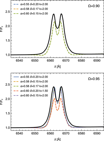
Figure 9. Synthetic Hα profiles computed at  and 0.95 with the radiative transfer code Bedisk, using the equatorial density structure obtained from the hydrodynamic code Hydwind, assuming spherical symmetry for the star. The adopted rotational velocity is given in the top right corner of each panel, and the line-force parameters used to calculate the density structure are given in the legend. Dashed and solid lines correspond to profiles with a lower and higher intensity than the ad hoc profile, respectively. The thick black line corresponds to the emission line profile computed with the ad hoc density structure. An inclination of
  is assumed for all profiles.
Download figure:
Standard image High-resolution image
Figure 10. Similar to Figure 9, but with the equatorial density structure calculated assuming an oblate shape for the star and neglecting the gravity darkening effect.
Download figure:
Standard image High-resolution image
Figure 11. Similar to Figure 9, but with the equatorial density structure calculated assuming an oblate shape for the star and including the gravity darkening effect.
Download figure:
Standard image High-resolution imageIn general, for our three scenarios, a combination of the highest values of α and δ from our grid is necessary to obtain an emission profile (with a low k) similar to our ad hoc model. The impact of α and δ on the wind parameters ( ) corresponding to the Ω-slow solution is similar to the behavior expected from the fast solution: smaller values of α have correspondingly smaller
  and v∞, while with smaller
  is smaller and v∞ is higher. For a given k, note that the α value has a greater impact on the final wind solution than the δ value.
Finally, as our hydrodynamic models have lower density values than the ad hoc model near the surface of the star (see Figure 6), the emission in the line wings of our model does not appear as strong as it does in the ad hoc models.
5. Summary and Discussion
We implemented the effect of high stellar rotation on line-driven winds by adopting a nonspherical central star and applying gravity darkening and the oblate finite disk correction factor to the m-CAK model. In order to numerically solve this improved model we developed an iterative procedure to calculate the oblate finite disk correction factor. This is a more general and robust model than the one developed by Müller & Vink (2014), because it retains the topology of the spherical m-CAK model, i.e., the model can be used to obtain either fast solutions (Friend & Abbott 1986), Ω-slow solutions (Curé 2004), or δ-slow solutions (Curé et al. 2011; Venero et al. 2016). When  , our wind model describes a two-component wind regime similar to that obtained by Curé et al. (2005).
From our results, we highlight the role of the oblate finite disk correction factor in the hydrodynamic, velocity, and density profiles, when these are compared with the spherical cases. In the case of the oblate finite disk correction factor calculated with gravity darkening,  varies by at least a factor of two between the equator and pole. Moreover, this particular derivation of
  results in a decrease in the mass-loss rate when compared with the factor obtained from the oblate case without gravity darkening. This is due to (1) the decrease in the temperature and (2) the fact that with increasing distance from the star, larger stellar surfaces with different temperatures than that in the radial-only direction, contribute.
Next we investigated the influence of oblateness and gravity darkening effects on the emergent Hα line profile from the circumstellar disk of a Be star. For this, we used the equatorial mass density distribution as input in the Bedisk code, neglecting the effects of radial and azimuthal velocities from the hydrodynamics in the radiative transport calculations.
We created a grid of equatorial Ω-slow models and the resulting grid of Hα profiles, for three different scenarios: (1) a spherically symmetric star with constant temperature, (2) an oblate star with constant temperature, and (3) an oblate star with gravity darkening. The results from the Hα grid were compared with the ad hoc line profile, which follows an  mass density distribution with n = 3.5 and
  .
.
We found an agreement between hydrodynamic and ad hoc Hα emission profiles (matching our 15% criterion) for values of  to
to  for spherical or oblate cases, and
  for the oblate case with gravity darkening, and values of
  and
and  . These results are for an ad hoc model with n = 3.5. In order to explore the variation in the line-force parameters and match ad hoc models with n = 3 (stronger emission line) and n = 4 (weaker emission line), we selected models based on our selection criteria, explained previously. We obtain good agreement between the oblate hydrodynamic models with gravity darkening and ad hoc models for values of
  when n = 3 and
  when n = 4 (see Figure 12). Models with n = 3 have slightly higher values of α and δ than models with n = 3.5.

Figure 12. Hα profiles: the ad hoc model for n = 3 is shown by the solid black line (upper panel). Other profiles from our grid of hydrodynamic models that satisfy our selection criteria are shown as dashed lines (see legend). The lower panel is same as the upper panel but for n = 4. See text for details.
Download figure:
Standard image High-resolution imageTo date, even though there is no self-consistent calculation of the line-force parameters for the Ω-slow solution, the values of k are roughly of order  for our scenarios 1 and 2; according to Puls et al. (2000), this would be a maximum value if line-overlap effects are neglected. We suggest, for scenario 3, that the large values found for k may be related to changes in the ionization structure and possible increments in the opacity of the absorption lines along the disk together with line-overlap effects.
On the other hand, to reproduce the emission line from an ad hoc model with lower values of the exponent n, we require higher values of k, hence multi-line scattering processes should be considered for these dense disks. Nevertheless, the values of k obtained in this study are closer to predicted values than those obtained by Silaj et al. (2014a). Finally, it is worth noting that for a given k the effect of α in the final wind solution is stronger than the effect of δ, generally.
Regarding the effect of the rotational velocity on the mass-loss rate, it is the corresponding equatorial mass density that mainly determines the strength of the emission profiles. However, for the same set of line-force parameters ( ), higher Ω values produce greater intensity of the emission line; this is valid for the scenarios assuming a spherical star and an oblate star of constant temperature. For the third scenario (an oblate star with gravity darkening), the maximum line intensity is attained at a value of
  . When Ω tends toward one, the emission is lower due to the decrease in effective temperature because of gravity darkening.
The contribution of the fast wind component is expected to have a negligible effect on the emission profile of the Hα line due to the low density of this region. In order to test this argument, we calculated the contribution to Hα using a fast wind solution with the following line-force parameters: α = 0.565, k = 0.32, and δ = 0.02, based on the calculations from Pauldrach et al. (1986) for a model with a similar  to our star. The hydrodynamic calculations with Hydwind for a spherical non-rotating case yield a mass-loss rate of 1.2 × 10⁻⁸
  yr−1 and a terminal velocity of 2350 km s−1. Then, this hydrodynamic solution is used as input in the radiative transfer code Fastwind (Puls et al. 2005) with the aim of obtaining the line profile accounting for the total contribution from the stellar photosphere and the fast wind (at all latitudes). We obtain an absorption line profile, which is then convolved with
  =339 km s−1. This profile is shown in Figure 13 by the black dashed line. Furthermore, this figure also shows the contribution to the Hα line from the stellar photosphere (absorption profile shown by the magenta dotted line) calculated by Bedisk and the emergent emission profiles from the stellar photosphere plus the disk (same as the lower panel of Figure 9). We note that the small difference between the absorption profiles demonstrates that, as expected, there is a minimal (negligible) contribution from the fast wind component.

Figure 13. Hα profiles: (a) absorption profile obtained for the non-disk region of a spherical rotating model at  , computed using the Fastwind code (black dashed line); (b) absorption profile of the stellar photosphere calculated by Bedisk (magenta dotted line); (c) emission profiles obtained for the disk plus photosphere calculated by Bedisk (see details in Figure 9). Note that the absorption profile calculated by Fastwind from the non-disk region includes the photospheric contribution, demonstrating that the overall contribution from the wind of the non-disk region is minimal.
Download figure:
Standard image High-resolution imageFinally, we have shown that the mass density distribution obtained from the Ω-slow wind solution (with  3), considering a more realistic scenario with gravity darkening, is able to reproduce Hα line emission features similar to those predicted by a power-law model. In addition, we also require a mechanism to provide Keplerian rotation within the disks of our models to produce reasonable profile shapes, which is an area of ongoing research in the field of Be stars.
In view of these new results, we are encouraged to further develop this line of research. In a future work, we plan to calculate, in a self-consistent way, the line-force parameters of this Ω-slow solution. In addition, it would be interesting to analyze the stability of this two-component wind in a 2D time-dependent frame that includes non-radial forces.
The authors would like to thank the referee, Dr. Joachim Puls, for his thoughtful comments and suggestions that helped to improve the paper significantly. This research was supported by the Canada–Chile Leadership Exchange Scholarship program from Government of Canada. I.A. acknowledges support from Fondo Institucional de Becas FIB-UV and Gemini-Conicyt 32120033. C.E.J. thanks support from NSERC, the National Sciences and Engineering Research Council of Canada. M.C. acknowledges support from Centro de Astrofísica de Valparaíso. L.C. and M.C. thank support from the project CONICYT+PAI/Atracción de capital humano avanzado del extranjero (folio PAI80160057). L.C. also acknowledges financial support from Universidad Nacional de La Plata (Programa de incentivos 11/G137) and from CONICET (PIP 0177). A.G. acknowledges support from the Swiss National Science Foundation through the Advanced Postdoc Mobility fellowship, project P300P2_158443. A.J. acknowledges support from CONICYT FONDECYT/POSTDOCTORADO 3150673, Nucleo Milenio ICR RC130003 and Proyecto Anillo ACT 1112.
Software: Hydwind (Curé 2004), Bedisk (Sigut & Jones 2007), Fastwind (Puls et al. 2005).
Appendix A: EoM for an Oblate Gravity-darkened Star
To derive the EoM to account for gravity darkening and the oblate distortion of the star in the radial direction, we start by analyzing the total (radial) acceleration (sum of effective and radiative accelerations) on the barotropic stellar layers, the photosphere. Following the work of Maeder & Meynet (2000), we have

where we have evaluated  with
with  . This is a reasonable approximation within the following context, due to the difficulty of knowing the exact value of κ, and because the upper photosphere of hot stars is dominated by electron scattering and to a lesser degree by line processes. As the line contribution is small below the sonic point we can generalize the expression of Maeder & Meynet (2000) for the wind region by adding an appropriate approximation for the line acceleration term that takes into account the increasing line force due to Doppler effects, allowing
  , i.e.,

In the m-CAK formalism, the radiative line acceleration can be expressed in terms of the continuum radiative acceleration due to Thomson scattering times a multiplication factor M(t), the so-called force-multiplier that is a function of the optical depth parameter t,

with

where  is the force-multiplier when the star is assumed to be a point source and
  is the finite disk correction factor for a spherical or oblate star (see, e.g., Lamers & Cassinelli 1999; Pelupessy et al. 2000). Then, considering the expression

we have

which, in turn, can eventually be generalized to consider gravity darkening if the local radiative flux and the appropriate finite disk correction factor are used. Thus, the radiative line acceleration can be expressed as

where  is a function of the local flux. Considering this expression, Equation (A2) can then be written in the following way:
Equation (A8) is more general and matches the conditions expected in the upper photosphere and in the wind, and is a function of the local Eddington ratio. Then, an EoM accounting for the gravity darkening and the oblate distortion of the star, with the variables  , and
, and  , can be derived in a similar way to Curé (2004) for a spherical case with a uniform surface brightness, using
  given by Equation (A8) in the equation of momentum,

It is important to note that in our study we use a simpler, but different approximation for  , i.e.,

where for small  ,
,  is not too different from
  . Our expression is similar to Equation (A8) if we assume that
  , as in the cases considered in this study (see Section 4.1). Finally, note that Equation (A8) needs to be carefully tested when it is applied to cases with considerable values of both
  and
and  .
.
Appendix B: Calculation of

The definition given for  in Equations (28) and (29) includes the ratio
  , which is not easily calculated because of the term
  . According to Maeder & Meynet (2000) this ratio can be expressed in terms of the rotational and critical rotational velocities as

where  is the classical critical rotational velocity independent of
  (Equation (15)).
  is the ratio of the actual volume of a star rotating at Ω to the volume of a sphere of radius
  . The term
  varies from 1 to 0.813 as
  goes from zero to
  . For low or moderate velocities this term tends to 1, but for higher rotational velocities it is necessary to calculate the value of
  . To this purpose, we perform a polynomial fit to the ratio
  , whose form is
with  . Now, the values of
  are easily calculated based on this polynomial fit. Figure 14 shows the comparison among the ratio
  , the polynomial fit given in Equation (B2), and the term
  as a function of Ω. From this figure, we observe that for values of Ω higher than ∼0.9 the term
  ceases to be a good approximation and the polynomial fit has excellent agreement with the ratio
  for the whole range of Ω.

Figure 14. Comparison among the ratio  (solid line), the polynomial fit for this ratio (dashed line, overlaid by the solid line) and the term
  (dotted line); all of these terms are dependent on Ω. The polynomial fit and the ratio
  are in excellent agreement. In addition, the term
  is a good approximation of
  for values of Ω lower than ∼0.9.
Download figure:
Standard image High-resolution imageFootnotes
- 6
Nevertheless, evolutionary calculations show that
depends slightly on Ω due to the small changes in internal structure (Maeder 2009). - 7
This is true for a barotropic case or if κ is the same over the entire stellar surface (Maeder 1999).
- 8
Note that Equations (24), (32), and (35) from Pelupessy et al. (2000) differ in the sign of the exponent α compared to our derivation, because of a typo in their equations.
