Abstract
The distribution of metals within a galaxy traces the baryon cycle and the buildup of galactic disks, but the detailed gas phase metallicity distribution remains poorly sampled. We have determined the gas phase oxygen abundances for 7138 H ii regions across the disks of eight nearby galaxies using Very Large Telescope/Multi Unit Spectroscopic Explorer (MUSE) optical integral field spectroscopy as part of the PHANGS–MUSE survey. After removing the first-order radial gradients present in each galaxy, we look at the statistics of the metallicity offset (ΔO/H) and explore azimuthal variations. Across each galaxy, we find low (σ = 0.03–0.05 dex) scatter at any given radius, indicative of efficient mixing. We compare physical parameters for those H ii regions that are 1σ outliers toward both enhanced and reduced abundances. Regions with enhanced abundances have high ionization parameter, higher Hα luminosity, lower Hα velocity dispersion, younger star clusters, and associated molecular gas clouds showing higher molecular gas densities. This indicates recent star formation has locally enriched the material. Regions with reduced abundances show increased Hα velocity dispersions, suggestive of mixing introducing more pristine material. We observe subtle azimuthal variations in half of the sample, but cannot always cleanly associate this with the spiral pattern. Regions with enhanced and reduced abundances are found distributed throughout the disk, and in half of our galaxies we can identify subsections of spiral arms with clearly associated metallicity gradients. This suggests spiral arms play a role in organizing and mixing the interstellar medium.
1. Introduction
The production and build-up of heavy elements from stellar nucleosynthesis over cosmic time has resulted in pronounced radial trends in chemical abundances within galaxies. This is commonly constrained by measuring the current gas phase oxygen abundance (metallicity) within H ii regions (Kennicutt & Garnett 1996). The predominantly negative radial trends in metallicity have been well established across large samples of galaxies (Zaritsky et al. 1994; Sánchez et al. 2014; Kaplan et al. 2016; Belfiore et al. 2017; Poetrodjojo et al. 2018), tracing the inside-out growth of galaxy disks (Boissier & Prantzos 1999).
In addition to tracking feedback and pollution from massive stars into the interstellar medium (ISM), metals play a key role in the cooling of the ISM, and drive changes in fundamental local ISM properties (e.g., gas-to-dust ratio, H i-to-H2 transition, CO-to-H2 conversion factor). Understanding the degree of chemical homogeneity in star-forming galaxies is key to making use of stellar metallicities for Galactic archaeology, including chemical tagging studies and assessments of burstiness and accretion events.
This purely radial picture may be an oversimplification because spiral arms, bars, and stellar feedback drive mixing and gas flows. This has been theorized to happen through bar-driven radial mixing (Di Matteo et al. 2013), spiral arm-driven large-scale systematic streaming motions (Grand et al. 2016; Sánchez-Menguiano et al. 2016), kiloparsec-scale mixing-induced dilution due to the spiral density waves passage (Ho et al. 2017), thermal and gravitational instabilities (Yang & Krumholz 2012; Petit et al. 2015), and interstellar turbulence (de Avillez & Mac Low 2002; Krumholz & Ting 2018). Many of these processes should affect azimuthal inhomogeneity in the gas phase abundances, which could then impact the local physical conditions that regulate star formation.
With typically only 10–100 H ii regions with measured abundances per galaxy (e.g., Pilyugin et al. 2014), detailed exploration of azimuthal trends has been unfeasible for large samples of galaxies, and the detailed gas phase metallicity distribution remains poorly understood. With the introduction of new wide-field optical integral field unit (IFU) spectrographs, it has become possible to fully sample the gas phase metallicity across galaxy disks. Large optical IFU projects that survey hundreds to thousands of galaxies (the Calar Alto Legacy Integral Field Area Survey, Sánchez et al. 2012; Mapping Nearby Galaxies at Apache Point Observatory, Bundy et al. 2015; Sydney-AAO Multi-object Integral-field spectrograph, Bryant et al. 2015) trade sample size for spatial resolution, approximately around kiloparsec spatial resolution. While having the obvious advantage of large statistical samples, this can introduce undesirable systematic effects when inferring metallicity, as multiple ionization sources can contribute within a single resolution element (Ho et al. 2018; Poetrodjojo et al. 2019).
Metallicity studies with optical IFU observations that isolate individual H ii regions (<100 pc scales) have so far been limited to individual objects. These studies have produced conflicting results, with some showing no evidence for significant large-scale azimuthal variations in relation to the spiral pattern (Kreckel et al. 2016), while other galaxies reveal clear enrichment patterns along spiral structures (Sánchez-Menguiano et al. 2016; Ho et al. 2017, 2018; Vogt et al. 2017). The Milky Way itself reveals tantalizing evidence for azimuthal metallicity variations (Balser et al. 2011, 2015).
The Physics at High Angular resolution in Nearby GalaxieS (PHANGS) collaboration20 aims to understand the interplay of the small-scale physics of gas and star formation with galactic structure and galaxy evolution. To this end, we are collecting observations of the molecular gas, ionized gas, and stellar populations within nearby (D < 17 Mpc) moderately inclined star-forming disk galaxies. To constrain the local and large-scale metallicities of these galaxies, we have begun a large observing program employing the Very Large Telescope/Multi Unit Spectroscopic Explorer (VLT/MUSE) to mosaic the central disk of 18 galaxies with optical IFU observations (PI: Schinnerer). Combined with our pilot survey that targeted NGC 628 (Kreckel et al. 2016, 2018), these 19 galaxies make up the PHANGS–MUSE survey.
We present here initial results from the PHANGS–MUSE survey using observations of the first eight completed galaxies. With ∼50 pc resolution across the central star-forming disks of these galaxies, our observations are well matched to the typical spatial scales of H ii regions (10–200 pc; Azimlu et al. 2011). Our MUSE observations can spatially isolate H ii regions and, using multiple line diagnostics, distinguish photoionized regions from other ionizing sources (diffuse ionized gas (DIG), supernova remnants, planetary nebulae, shocks, outflows, and extended ionization from an active galactic nuclei). This combination of high spatial resolution with multiple line diagnostics mapped across the galaxy disks allows us to take a statistical approach to characterize metallicity variations across galaxy disks and relate these to the local physical conditions of the ISM.
Section 2 presents the data we use and describes the construction of our H ii region catalogs. In Section 3 we detail how we use emission lines to infer the physical conditions of H ii regions, particularly the metallicity and ionization parameter. Section 4 presents our results on the trends in metallicity with local physical conditions, the subtle evidence we observe for azimuthal variations, and a brief discussion of the impact of bars on the metal distribution. Section 5 discusses the implications of our results and we conclude in Section 6.
2. Data
2.1. Observations
We use the MUSE spectrograph (Bacon et al. 2010) at the VLT to mosaic the central star-forming disks of eight nearby spiral galaxies (Table 1) as part of the PHANGS–MUSE large observing program (PI: Schinnerer). This powerful optical IFU provides a 1′ × 1′ field of view with 02 pixels and a typical spectral resolution of ∼2.5 Å over the nominal wavelength range, covering 4800–9300 Å. Our sample of eight galaxies includes observations of NGC 628, which have been described previously (Kreckel et al. 2016, 2018). For our large program observations, each position was observed in four rotations, with two sky pointings, and a total on-source integration time of 43 minutes. For NGC 628 we used slightly different integration times (43–50 minutes). The center pointing for NGC 2835 was observed as part of the MUSE Atlas of Disks survey (Erroz-Ferrer et al. 2019), with 60 minute exposure time. NGC 4254 and NGC 4535 were observed using the wide-field adaptive optics (AO) mode. We present here results using the first eight completed galaxies. Table 1 summarizes the main properties of the galaxy sample, the angular resolution achieved in the observations, the number of H ii regions in each galaxy, and the physical size of the survey area covered in the disk.
Table 1. Key Parameters of Our Galaxy Sample
| Name | D | Type | Log10(M*) | Log10(SFR) | PAa | ib | R25c | Angular | Physical | Number of | Survey |
|---|---|---|---|---|---|---|---|---|---|---|---|
| Resolution | Resolution | H ii Regions | Area | ||||||||
| (Mpc) | (M⊙) | (M⊙ yr−1) | (deg) | (deg) | (arcmin) | (arcsec) | (pc) | (kpc2) | |||
| NGC 0628 | 9.77 ± 0.82 | Sc | 10.2 | 0.26 | 20.9 | 8.7 | 5.0 | 1.0 | 47 | 1277 | 96 |
| NGC 1087 | 14.4 ± 4.8 | SBc | 9.8 | 0.05 | 177.3 | 41.3 | 1.5 | 1.0 | 70 | 679 | 105 |
| NGC 1672 | 11.9 ± 4.0 | SBb (S) | 10.2 | 0.48 | 135.7 | 37.5 | 3.1 | 0.8 | 46 | 880 | 95 |
| NGC 2835 | 10.1 ± 3.4 | SBc | 9.6 | −0.08 | 1.6 | 47.8 | 3.2 | 0.9 | 44 | 699 | 60 |
| NGC 3627 | 10.6 ± 0.9 | SBb (S3) | 10.6 | 0.55 | 174.1 | 55.0 | 5.1 | 1.0 | 51 | 692 | 76 |
| NGC 4254 | 16.8 ± 5.6 | Sc | 10.5 | 0.74 | 67.7 | 37.8 | 2.5 | 0.7 | 57 | 1824 | 191 |
| NGC 4535 | 15.8 ± 2.3 | SBc | 10.4 | 0.35 | 179.8 | 40.7 | 4.1 | 0.5 | 38 | 864 | 126 |
| IC 5332 | 9.95 ± 3.3 | SBc | 9.6 | −0.31 | 74.7 | 24.0 | 3.0 | 0.8 | 39 | 223 | 42 |
Notes. The galaxy parameters are adopted from the z0mgs (z = 0 multiwavelength galaxy survey; Leroy et al. 2019) database (https://github.com/akleroy/z0mgs), where the original references can be found. R25 taken from HYPERLEDA.
aPosition angle. bInclination. cthe galactic radius at 25 mag arcsec−2.Download table as: ASCIITypeset image
Angular resolution varies between galaxies from 05 (for the AO mode) to 1
0, and can vary slightly between fields (typically less than 0
2) and as a function of wavelength (0
1–0
2 across the whole wavelength range). At the distances of our sample, this resolution corresponds to physical scales of 40–70 pc. As we integrate the spectrum over each entire H ii region, the slight variations in seeing should not impact our results.
Observations are reduced using a pipeline built on esorex and developed by the PHANGS team.21 Between five and 12 MUSE pointings are observed per galaxy and each is reduced individually to produce a data cube. As observations were taken under mostly photometric conditions, no additional absolute flux calibration corrections are applied except for on NGC 628 (as described in Kreckel et al. 2017, 2018). As all metallicity diagnostics are inferred from line ratios, our main results depend only on the relative flux calibration and are insensitive to the absolute flux calibration.
The relative astrometric solution across each MUSE field of view is excellent (∼004). A single additional absolute astrometric correction for each pointing is obtained by comparing the white light image with reference images. For the majority of our galaxies we used SDSS r-band images as our reference. For NGC 1672 we used an R-band image acquired as part of the PHANGS Hα imaging survey (A. Razza et al. 2019, in preparation) with astrometry determined from Gaia (Gaia Collaboration et al. 2018), while for NGC 2835 we used an R-band image coming from the Danish 1.54 m telescope (Larsen & Richtler 1999) with an astrometric solution determined by astrometry.net. For IC 5332 we used an R-band image from the CTIO LVL optical survey (Cook et al. 2014). To determine the astrometric solution, both the MUSE image and the reference image were analyzed with the IDL procedure “find” (an adaptation of DAOPHOT) to identify point-like sources in the image. As our MUSE fields are entirely contained within the disk of the galaxy, these often do not correspond to stars but to unresolved star-forming knots within the disk. We then cross-matched these point sources, typically finding 5–20 matches per MUSE field, and applied the average offset. Typical shifts are 1″–2″, and systematic uncertainties are estimated to be ∼0
2, but are dependent on the absolute accuracy of the astrometric solution in the reference image.
In order to morphologically identify the H ii regions by their Hα line emission, we first produce maps covering the full field of view. All data cubes are processed using the IDL toolkit LZIFU (Ho et al. 2016) to fit stellar spectral templates and extract emission line fluxes. The resulting emission line maps from all pointings are combined to produce full coverage emission line maps for each galaxy. Three color images are presented for all eight galaxies in an atlas (Appendix A, Figures 10–17). We reach a typical 3σ surface brightness sensitivity for Hα of 1.5 × 10⁻¹⁷ erg s−1 cm−2 arcsec−2.
2.2. H ii Region Catalogs
Hα emission line maps are analyzed with H iiphot (Thilker et al. 2000), which has been designed to morphologically isolate H ii regions from DIG, and provide a 2D mask that identifies separate regions within the map. After identifying “seeds” for the H ii region peaks, their boundaries are set by identifying where the slope of the Hα surface brightness distribution meets user-defined termination criteria. We adjust the settings of H iiphot to produce realistic H ii region sizes and shapes across the eight galaxies in this sample, changing only the background surface brightness sensitivity level between galaxies. We then use the resulting mask to extract integrated spectra from the data cubes. As a check, we repeated our analysis using spectra extracted from a circular 1″ diameter aperture centered at the position of each identified region. The derived line ratios and metallicities agree with those calculated from the H ii region catalogs within 0.01 dex for 84% of the sample. Thus, the exact boundaries set and choice of tuning parameters for H iiphot have only a small effect.
These integrated region spectra are then fit with GANDALF (Gas AND Absorption Line Fitting; Sarzi et al. 2006), which simultaneously fits the stellar continuum using pPXF (penalized Pixel-Fitting; Cappellari & Emsellem 2004; Cappellari 2017) and the emission line fluxes (Hβ, [O iii] λ4959,5007, [OI]λ6300, Hα, [N ii]λ6548,6583, [S ii]λ6716,6731, [S iii]λ9069). Emission lines are fit without tying together the line centers or kinematics, in order to account for the varying spectral resolution. We fit the stellar continuum with stellar population models taken from the Tremonti et al. (2004) library of Bruzual & Charlot (2003) templates across a range of ages (5 Myr–11 Gyr) and metallicities (Z = 0.004, 0.02, and 0.05). Our results do not change significantly if we use another stellar population model (e.g., MIUSCAT stellar population synthesis models; Vazdekis et al. 2012). All line fluxes are corrected for extinction using the Balmer decrement to infer the reddening, assuming case B recombination and Te = 104 K, and applying the Fitzpatrick (1999) extinction law assuming a value of RV = 3.1. This is relatively insensitive to the assumed electron temperature, with variations by a factor of two resulting in only ∼0.1 magnitude difference in the V-band extinction. Using a different extinction law (e.g., Cardelli et al. 1989) does not significantly change our results.
We then employ a number of criteria to produce our H ii region catalog.
- 1.Any region within 5″ of the edge of the full mosaic is removed to ensure the entire region is contained within the field of view. This excludes ∼7% of the regions.
- 2.A signal-to-noise ratio S/N > 5 is required for all strong emission lines used to infer the metallicity (Hβ, [O iii], Hα, [N ii], [S ii]), which excludes a further ∼5% of the regions.
- 3.Two BPT (Baldwin et al. 1981) emission line ratio diagnostics are employed to ensure the excitation is consistent with photoionization by massive stars (see Appendix B). In the [O iii]/Hβ versus [N ii]/Hα diagnostic, we require regions to be consistent with the stringent empirical line (Kauffmann et al. 2003). In the [O iii]/Hβ versus [S ii]/Hα diagnostic, we require regions to be consistent with the Kewley et al. (2001) line. These BPT diagnostics remove another 7% of the regions.
- 4.While the above remove the majority of planetary nebulae and supernova remnants, we further remove 15 additional regions (∼0.1% of the total catalog) with large (>100 km s−1) velocity dispersion that are likely compact supernova remnants.
These cuts together remove a total of ∼10%–20% of regions from each galaxy, with the remainder comprising our H ii region catalogs (Table 2). We list the total number of H ii regions identified for each galaxy (ranging from 200 to 2000) in Table 1.
Table 2. H ii Region Catalog (Online Only, Example Data for three Regions)
| Parameter | Unit | |||
|---|---|---|---|---|
| ID | ngc628_0001 | ngc628_0002 | ngc628_0003 | |
| R.A.a | degrees | 24.175116 | 24.194861 | 24.170381 |
| Decl.a | degrees | 15.784356 | 15.788300 | 15.793022 |
| R/R25 | 0.01 | 0.25 | 0.12 | |

|
mag | 0.00 ± 0.02 | 0.30 ± 0.05 | 0.40 ± 0.03 |
| L(Hα) | 1e36 erg s−1 | 4.56 ± 0.03 | 5.08 ± 0.05 | 5.01 ± 0.04 |
| Hβ | 1e–16 erg s−1 cm−2 | 1.68 ± 0.16 | 1.55 ± 0.37 | 1.54 ± 0.22 |
| [O iii]λ5007 | 1e–16 erg s−1 cm−2 | 0.69 ± 0.08 | 1.00 ± 0.25 | 0.32 ± 0.08 |
| Hα | 1e–16 erg s−1 cm−2 | 3.99 ± 0.21 | 4.45 ± 0.54 | 4.39 ± 0.33 |
| [N ii]λ6583 | 1e–16 erg s−1 cm−2 | 1.73 ± 0.10 | 1.40 ± 0.19 | 1.77 ± 0.15 |
| [S ii]λ6716 | 1e–16 erg s−1 cm−2 | 0.69 ± 0.05 | 1.04 ± 0.13 | 0.64 ± 0.05 |
| [S ii]λ6731 | 1e–17 erg s−1 cm−2 | 5.04 ± 0.38 | 6.90 ± 0.94 | 3.82 ± 0.37 |
| [S iii]λ9069 | 1e–17 erg s−1 cm−2 | 6.93 ± 0.70 | 1.93 ± 0.53 | 1.68 ± 0.30 |
| 12+log(O/H) | 8.57 ± 0.05 | 8.46 ± 0.13 | 8.61 ± 0.08 |
Note.
aJ2000Only a portion of this table is shown here to demonstrate its form and content. A machine-readable version of the full table is available.
Download table as: DataTypeset image
By eye, H iiphot does an excellent job of identifying H ii regions (Figures 10–17), isolating the individual Hα peaks and segmenting clustered complexes into discrete H ii regions. However, it is also apparent that in rare circumstances the termination criteria are not correctly met at the H ii region boundary, which results in a small number of regions that grow to unphysical sizes of up to >200 pc (<1% of regions). This is particularly clear for some of the inter-arm H ii regions (e.g., on the eastern side of NGC 628). Taking the area of the irregular mask defining each H ii region, we infer a size corresponding to a circular radius that would encompass the same area. Looking at this H ii region size distribution (Figure 1), we see the expected power-law behavior (e.g., Azimlu et al. 2011) up to 120 pc sizes, suggesting these unphysically large regions are not introducing a significant bias, and we retain these regions in our sample.
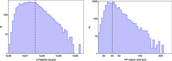
Figure 1. Distribution of extinction-corrected Hα luminosities (left) and H ii region sizes (right) for the full H ii region sample across all galaxies. Here, we have computed the sizes as the circular radius which would contain the same area as covered by the H ii region masks. Dashed lines show the approximate completeness limit corresponding to the most distant galaxy in our sample. Both distributions exhibit the expected power-law behavior.
Download figure:
Standard image High-resolution imageThe extinction-corrected Hα luminosity function for our full sample is presented in Figure 1, and shows the expected power-law slope with a break at ∼1039 erg s−1 (Bradley et al. 2006). Based on our 5σ Hα sensitivity for 1″ diameter regions, we estimate typical completeness limits of L(Hα) ≃ 4 × 1037 erg s−1, though they vary given the range in galaxy distances. This is roughly comparable to the ionizing flux produced by a single O5V star (Schaerer & de Koter 1997). All galaxies are fairly face-on or only moderately inclined (i < 55°), and the typical V-band extinctions we infer are quite moderate (1.0 ± 0.3 mag), so we do not expect that we are missing a significant fraction of bright H ii regions.
All H ii region positions, line fluxes, and associated uncertainties are tabulated in Table 2. The full table is available as supplementary data, with only a small sample shown here. Positions reflect the geometric center of each identified H ii region, without any intensity weighting. The integrated Hα luminosity and all emission line fluxes have been extinction corrected, as described above, and are listed in the table in absolute flux units.
2.3. Ancillary Data
We compare our MUSE results to spectroscopic imaging of the CO (2−1) line from the PHANGS–ALMA survey (PI E. Schinnerer). The sample selection, observations, and data reduction for PHANGS–ALMA are described in Leroy et al. (2019). Briefly, we observed each target with ALMA’s main array in a compact configuration and with the 7 m arrray and single dish (“total power”) telescope. The combination of these observations yield CO line data cubes with resolution ≈1″−2″ and sensitivity to emission on all spatial scales. The standard PHANGS–ALMA products include integrated intensity (“moment 0”) maps, maps of the peak intensity (“Tpeak”) at any velocity along each line of sight, intensity-weighted mean intensity (“moment 1”) maps, and several line width estimates. Here we use the velocity dispersion estimated from the rms scatter of emission about the intensity-weighted mean velocity (i.e., the “moment 2” line width). Use of an alternative parameterization of the molecular gas line width does not significantly change our results. The kinematic measurements at high resolution require reasonable S/N, and so have limited coverage in IC 5332 and NGC 2835, which both have relatively low stellar mass and correspondingly weak CO emission. Maps for six of our eight targets have appeared before (Kreckel et al. 2018; Sun et al. 2018; Utomo et al. 2018), and we refer the reader to those papers for additional visualizations and details.
The surface brightness sensitivity of the CO maps becomes higher at coarser resolution. At the ≈7″ resolution of ALMA’s 7 m telescopes, we detect essentially all CO emission from all targets, including IC 5332 and NGC 2835. When computing the general distribution of molecular gas, we use a low-resolution, high-completeness version of the moment 0 maps created at this lower resolution of the 7 m data.
FUV emission was observed by the Galaxy Evolution Explorer (GALEX) satellite, with all maps taken from the GALEX archive using the longest exposure time available for each galaxy. Most are taken from guest investigator programs with 1.7–21 ks exposures. NGC 1087 was observed as part of the Medium Imaging survey with a 3 ks exposure, and NGC 1672 was observed as part of the Nearby Galaxy Survey (Gil de Paz et al. 2007) with a 2.7 ks exposure. Only NGC 2835 has a significantly shorter (100 s) exposure time from the All-Sky Imaging Survey. Images are used at the native 45 angular resolution. FUV fluxes are extinction corrected based on the observed Balmer decrement assuming a Fitzpatrick (1999) extinction law, including a factor of two decrease in the reddening
 assumed for the stellar UV emission in relation to the nebular Hα emission (Kreckel et al. 2013).
3. H ii Region Physical Conditions
We present a sample of eight galaxies with unprecedented statistics, identifing a total of 7138 H ii regions, with measurement of 200–2000 H ii region metallicities per galaxy. We outline here our method for inferring the gas phase oxygen abundance (metallicity), and present the radial gradients observed within each galaxy.
3.1. Strong Line Metallicities
There is a long-standing debate in the literature regarding how best to calculate the gas phase oxygen abundances using only strong emission lines, where the H ii region electron density and temperature cannot be directly measured. Empirical calibrations are determined by comparing different strong line ratios with metallicities calculated from faint auroral line detections that are used to estimate the electron temperature and therefore “directly” measure ionic abundances. This Te method is often viewed as the “gold standard” for determining metallicity (Skillman 1989; Garnett 2002; Bresolin 2007; Stasińska et al. 2007; Berg et al. 2015; McLeod et al. 2019; but see Blanc et al. 2019). Alternatively, theoretical calibrations are determined by comparing different strong line ratios with photoionization model grids. For the same data sets, systematic offsets of 0.2 dex are found between empirical and theoretical calibrations (Kewley & Ellison 2008; Blanc et al. 2015). While we do detect auroral line emission in ∼20–50 H ii regions per galaxy (Ho et al. 2019), this is an order of magnitude fewer than the number of regions for which we can identify and measure strong line fluxes.
As our MUSE observations do not cover the [O ii]λ3727 emission line, only a limited number of strong line prescriptions are available for determining the metallicity (see Appendix C). All calculations in this paper adopt the empirical Pilyugin & Grebel (2016) S-calibration (Scal). It relies on the following three standard diagnostic line ratios:
![${N}_{2}={I}_{[{\rm{N}}{\rm{II}}]\lambda 6548+\lambda 6584}/{I}_{{\rm{H}}\beta }$](https://content.cld.iop.org/journals/0004-637X/887/1/80/1/apjab5115ieqn3.gif) ,
,
![${S}_{2}={I}_{[{\rm{S}}{\rm{II}}]\lambda 6717+\lambda 6731}/{I}_{{\rm{H}}\beta }$](https://content.cld.iop.org/journals/0004-637X/887/1/80/1/apjab5115ieqn4.gif) ,
,
![${R}_{3}={I}_{[{\rm{O}}{\rm{III}}]\lambda 4959+\lambda 5007}/{I}_{{\rm{H}}\beta }$](https://content.cld.iop.org/journals/0004-637X/887/1/80/1/apjab5115ieqn5.gif) .
.
Here we have measured only the stronger line in both the [O iii] and [N ii] doublets and assume a fixed ratio of 3:1. The Scal prescription is defined separately over the upper and lower branches in log N2, with almost all H ii regions in our sample falling on the upper branch (log N2 ≥ −0.6), as

and the lower branch (log N2 ≤ −0.6) is calculated as

We prefer this metallicity calibration as it shows small intrinsic scatter versus the auroral line metallicities for the same regions. This is quoted to be <0.1 dex across the full metallicity range (Pilyugin & Grebel 2016). A more recent investigation comparing metallicity calibrations reports systematic ∼0.17 dex scatter for this prescription, as good as or better than all other tested calibrations, and similar to the best results achieved from a machine-learning approach (Ho 2019). Furthermore, Scal relies on a combination of three emission line ratios, an important improvement over past calibrations, which allows it to correct for dependences with the ionization parameter (Pilyugin & Grebel 2016). Finally, we find that this prescription systematically shows the smallest scatter (0.03–0.05 dex) around the radial metallicity gradient compared to alternative metallicity prescriptions (see Appendix C). While this does not necessarily mean this method is the most accurate, we do not expect any method to imply a scatter lower than the true scatter. Some further discussion on this point is presented in Section 5.2. The Scal metallicity for each H ii region is listed in Table 2. Two-dimensional maps of the identified H ii regions, each colored by the measured metallicity, are shown in Figures 10–17.
While a detailed exploration of the differences between empirical and theoretical metallicity calibrations is beyond the scope of this paper, we find very good qualitative agreement between the metallicity trends and correlations presented here with an analysis performed using the Dopita et al. (2016) photoionization model based N2S2 prescription. The reported trends and correlations also do not change qualitatively when using the Bayesian inference code IZI (Blanc et al. 2015) to derive the joint and marginalized posterior probability density functions for metallicity and ionization parameter given a set of observed line fluxes and an input photoionization model. This further increases our confidence in the robustness of the presented results. We do note that our results change qualitatively when using the Marino et al. (2013) O3N2 and N2 calibrations. However, because these use smaller dimensionality in the line ratios, we believe both of these alternative calibrations retain the degeneracy between metallicity and ionization parameter, enough to cloud the subtle trends presented here. Select results using additional calibrations are shown in Appendix C, along with a more detailed discussion of how results presented in this paper would change if the analysis was performed with an alternative calibration.
3.2. Radial Metallicity Gradients
The rightmost panels in our atlas (Appendix A, Figures 10–17) map the Scal metallicity of each H ii region in each galaxy. These figures show clearly both the different mean metallicity between galaxies (linked to the mass–metallicity relation; Tremonti et al. 2004), and also the known trend of metallicity decreasing with galactic radius. On top of this, however, there appear to be higher-order trends with suggestive links to galactic features like bars and spiral arms.
We perform a first-order linear fit to the radial gradient (Figure 2). We include in the fit the determined errors for all line flux measurements, including the uncertainty in the flux measurements due to the uncertainty in our measurement of  . We exclude the inner 0.1R25 when performing our fit, as it could be biased by nuclear ionization sources. We also calculate the running median in radial bins, and find very good agreement with our simple linear fit. Coefficients for radial gradients in each galaxy are shown in Figure 2 and tabulated in Appendix C (Table 3). All galaxies show small (0.03–0.05 dex) systematic scatter after accounting for the radial trends.

Figure 2. Radial metallicity gradients for all eight galaxies in our sample. All metallicities are calculated using the Pilyugin & Grebel (2016) Scal strong line prescription. Uncertainties in the metallicity from propagating line flux errors (lower left corners) are similar (0.02–0.3 dex) to the systematic uncertainties in the calibration (0.02 dex). Overplotted are linear fits (excluding the central 0.1 R25) to the radial gradient (solid black), with the uncertainty in the fit shown as a gray bar, and the median calculated for 0.05 R25 wide radial bins (dotted red). The two radial trends show agreement overall. NGC 1672, NGC 3627 and NGC 4535 exhibit flat or slightly increasing gradients, but note that all three galaxies contain a pronounced stellar bar that extends across much of the field of view (see Figures 10–17). The remaining galaxies exhibit declining gradients. All galaxies show small (0.03-0.05 dex) scatter about the radial gradient.
Download figure:
Standard image High-resolution imageTable 3. Radial Gradient Fits (in Appendix C)
| Scal | N2S2 (D16) | O3N2 (M13) | N2 (PP04) | |||||||||||||
|---|---|---|---|---|---|---|---|---|---|---|---|---|---|---|---|---|
| Name | R0 | Gradient | Gradient | σ(O/H) | R0 | Gradient | Gradient | σ(O/H) | R0 | Gradient | Gradient | σ(O/H) | R0 | Gradient | Gradient | σ(O/H) |
| (dex | (dex | (dex) | (dex | (dex | (dex) | (dex | (dex | (dex) | (dex | (dex | (dex) | |||||
 ) ) |
kpc−1) |
 ) ) |
kpc−1) |
 ) ) |
kpc−1) |
 ) ) |
kpc−1) | |||||||||
| ngc628 | 8.556 | −0.191 | −0.0412 | 0.05 | 8.771 | −0.456 | −0.0913 | 0.11 | 8.611 | −0.164 | −0.0329 | 0.05 | 8.508 | −0.009 | −0.0018 | 0.04 |
| ±0.005 | ±0.018 | ±0.0037 | ±0.011 | ±0.041 | ±0.0082 | ±0.005 | ±0.017 | ±0.0035 | ±0.003 | ±0.012 | ±0.0025 | |||||
| ngc1087 | 8.483 | −0.144 | −0.0994 | 0.03 | 8.580 | −0.251 | −0.1676 | 0.08 | 8.542 | −0.118 | −0.0784 | 0.04 | 8.526 | −0.102 | −0.0678 | 0.02 |
| ±0.003 | ±0.006 | ±0.0048 | ±0.009 | ±0.017 | ±0.0114 | ±0.005 | ±0.009 | ±0.0061 | ±0.003 | ±0.005 | ±0.0035 | |||||
| ngc1672 | 8.563 | −0.056 | −0.0199 | 0.03 | 8.737 | −0.089 | −0.0287 | 0.10 | 8.571 | −0.074 | −0.0238 | 0.04 | 8.567 | −0.052 | −0.0169 | 0.03 |
| ±0.003 | ±0.007 | ±0.0022 | ±0.009 | ±0.019 | ±0.0062 | ±0.004 | ±0.009 | ±0.0030 | ±0.002 | ±0.005 | ±0.0017 | |||||
| ngc2835 | 8.565 | −0.516 | −0.1586 | 0.04 | 8.734 | −0.907 | −0.2834 | 0.09 | 8.598 | −0.401 | −0.1253 | 0.06 | 8.567 | −0.319 | −0.0997 | 0.03 |
| ±0.004 | ±0.012 | ±0.0038 | ±0.010 | ±0.027 | ±0.0085 | ±0.006 | ±0.018 | ±0.0056 | ±0.003 | ±0.009 | ±0.0028 | |||||
| ngc3627 | 8.528 | 0.056 | 0.0095 | 0.03 | 8.733 | 0.084 | 0.0164 | 0.07 | 8.571 | 0.108 | 0.0212 | 0.04 | 8.506 | 0.041 | 0.0080 | 0.03 |
| ±0.004 | ±0.016 | ±0.0031 | ±0.009 | ±0.034 | ±0.0066 | ±0.005 | ±0.019 | ±0.0037 | ±0.004 | ±0.015 | ±0.0029 | |||||
| ngc4254 | 8.592 | −0.104 | −0.0425 | 0.03 | 8.873 | −0.241 | −0.0966 | 0.08 | 8.632 | −0.142 | −0.0568 | 0.04 | 8.513 | 0.000 | 0.0001 | 0.04 |
| ±0.002 | ±0.004 | ±0.0019 | ±0.004 | ±0.011 | ±0.0045 | ±0.002 | ±0.006 | ±0.0022 | ±0.002 | ±0.005 | ±0.0020 | |||||
| ngc4535 | 8.579 | −0.091 | −0.0244 | 0.04 | 8.844 | −0.258 | −0.0628 | 0.09 | 8.626 | −0.082 | −0.0200 | 0.05 | 8.471 | 0.129 | 0.0314 | 0.04 |
| ±0.006 | ±0.018 | ±0.0045 | ±0.012 | ±0.041 | ±0.0100 | ±0.006 | ±0.021 | ±0.0051 | ±0.005 | ±0.018 | ±0.0043 | |||||
| ic5332 | 8.514 | −0.401 | −0.1362 | 0.05 | 8.671 | −0.717 | −0.2391 | 0.11 | 8.574 | −0.251 | −0.0836 | 0.07 | 8.520 | −0.224 | −0.0746 | 0.03 |
| ±0.010 | ±0.035 | ±0.0119 | ±0.022 | ±0.076 | ±0.0255 | ±0.014 | ±0.049 | ±0.0163 | ±0.006 | ±0.020 | ±0.0065 | |||||
Download table as: ASCIITypeset image
3.3. Ionization Parameter
The structure of an H ii region is set by the ionizing radiation provided by the central star(s) acting on the surrounding ISM. For the simplistic case of a spherically symmetric H ii region that has achieved equilibrium, this balance can be parameterized in terms of the dimensionless ionization parameter, U = Q(H0)/(4πR2nc), where Q(H0) is the number of hydrogen-ionizing photons (E > 13.6 eV) emitted per second, R is the empty (wind-blown) radius, n is the hydrogen density, and c is the speed of light. Direct interpretation of this parameter is challenging, as there are degeneracies between the ionizing flux produced by a single very young star as opposed to a cluster of slightly older stars. Moreover, detailed studies of resolved H ii regions reveal asymmetric and broken shells surrounding the ionizing sources (Pellegrini et al. 2011, 2012). Nonetheless, this parameter is still useful as it encodes information about the local physical conditions, with higher values typically indicating a stronger ionizing source or a lower ionized gas density.
Photoionization modeling has been used to constrain the ionization parameter through different diagnostic line ratios (Kewley & Dopita 2002; Dors et al. 2011). [O iii]λ5007/([O ii]λ3726+[O ii]λ3729) has frequently been used to constrain the ionization parameter, but has a strong dependence on metallicity. ([S iii]λ9069+[S iii]λ9532)/([S ii]λ6716+[S ii]λ6731) also shows a positive correlation with ionization parameter, and is a much more direct diagnostic of the ionization parameter, with only a weak dependence on metallicity and no sensitivity to the ISM pressure between between 4 cm−3 K < log(P/k) < 7 cm−3 K. This makes [S iii]/[S ii] the best ionization parameter diagnostic available in the optical, although the long-wavelength [S iii]λ9069,9532 lines have not often been observed. With MUSE we observe the [S iii]λ9069 line flux, and for our calculations we assume the fixed theoretical line ratio of [S iii]λ9532/[S iii]λ9069 = 2.5 (Vilchez & Esteban 1996), which is well determined from the transition probabilities. Figure 3 presents the radial gradients of [S iii]/[S ii], tracing the radial ionization parameter gradient. All gradients are very close to being flat within the inner part of the galaxy disks, as also found in Poetrodjojo et al. (2018).

Figure 3. Radial trends in ionization parameter (as traced by [S iii]/[S ii]) for all eight galaxies in our sample. Typical uncertainties in [S iii]/[S ii] are 0.05 (∼10%). Overplotted are linear fits (excluding the central 0.1 R25) to the radial gradient, with the 1σ uncertainties shown as a gray bar, and a median calculated for radial bins (dotted red). Most galaxies are consistent with a flat gradient.
Download figure:
Standard image High-resolution imageWe choose in this paper to present results related to the ionization parameter directly in terms of the observed line ratios, and remind the reader that a positive linear correlation is expected between log([S iii]/[S ii]) and U. Various prescriptions (e.g., Kewley & Dopita 2002; Dors et al. 2011) are available in the literature to convert a measured [S iii]/[S ii] line ratio to a value for U (or q = U/c); however they differ by an order of magnitude.
3.4. Diffuse Ionized Gas
DIG is seen in disk galaxies as an extended, relatively smooth background in emission line maps (Zurita et al. 2000). DIG contributes ∼40%–60% of the total Hα flux observed within any disk galaxy (Ferguson et al. 1996; Zurita et al. 2000; Thilker et al. 2002; Oey et al. 2007; Chevance et al. 2019), and even at the location of individual H ii regions has been shown to contribute at significant levels (20%–80%, Kreckel et al. 2016) that vary by local environment (e.g., arm/interarm). DIG is detected predominantly in the Hα, Hβ, [N ii] and [S ii] line maps, as these lines are strongly emitted in the low-density, high-temperature diffuse gas (Haffner et al. 2009). One major advantage of the high physical resolution of the maps employed in this work is that we can spatially distinguish H ii regions from the surrounding diffuse emission, which when blended over larger apertures has been shown to artificially flatten metallicity gradients (Poetrodjojo et al. 2019). The emission line fluxes and Hα luminosities reported here do not include any correction for the DIG background contributing to the integrated line flux, as seen in projection against any given H ii region. A major goal of the PHANGS collaboration is to develop and compare spectroscopic, morphological, and hybrid estimators of the DIG. At this time, we lack such rigorous methods to identify the DIG, and we view imposing such a correction as premature. As such, we have chosen to exclude such a correction from our reported line fluxes and subsequent analysis as it would strongly depend on our choice of H ii region boundary.
We estimate the effect this un-subtracted diffuse background could have on our inferred metallicities by using our emission line maps to measure the median line flux per pixel over an annular aperture surrounding each H ii region in our masks. The aperture size is scaled corresponding to the observed H ii region size, and is typically 06–2″ wide. Here we have masked any neighboring H ii regions to ensure minimal contamination of our measurement. Our DIG flux fractions are consistent with those obtained through other methods (Chevance et al. 2019; Hygate et al. 2019). As in Kreckel et al. (2016), we observe order of magnitude variations in DIG surface brightness across each disk at the locations of H ii regions, with the most Hα luminous H ii regions showing lower fractional DIG contribution (∼10%–20%) compared to fainter H ii regions, with contributions as high as ∼80%. For this calculation, we identify a subset of regions where the Hα DIG background is 50% or less. For all emission lines we then subtract the estimated DIG level from our H ii region line fluxes. We then use these DIG-subtracted line fluxes to calculate the metallicity as described in Section 3.1. We find that subtracting the DIG emission would result in a slight (∼0.02 dex) systematic increase in our inferred metallicities, and an increased systematic scatter (0.05–0.1 dex) across the sample. This increased scatter washes out some of the weaker azimuthal variations we see, but does not qualitatively change the strongest trends we observe in NGC 1672 and NGC 1087.
This diffuse background more strongly impacts our inferred ionization parameters via our measurement of the [S iii]/[S ii] line ratios, as [S iii] is predominantly confined to the H ii regions while [S ii] is emitted strongly in the diffuse gas. Correcting for the DIG contribution to the [S ii] line would result in a ∼70% increase in the [S iii]/[S ii] line ratios but does not qualitatively change the trends described in the following sections.
4. Results
4.1. Trends with Local Physical Conditions
Within each of our galaxies we observe a positive correlation between the metallicity and ionization parameter of the H ii regions (Figure 4), with an offset between different galaxies that is set by the difference in stellar mass of the systems. As the ionization parameter shows no radial gradient, this is not simply a result of correlated observables. Similarly, while many emission line diagnostics can be influenced by both the metallicity and the ionization parameter, we have selected a metallicity prescription that has been defined by carefully fitting a three-dimensional parameter space of diagnostic line ratios in order to minimize the degeneracies.
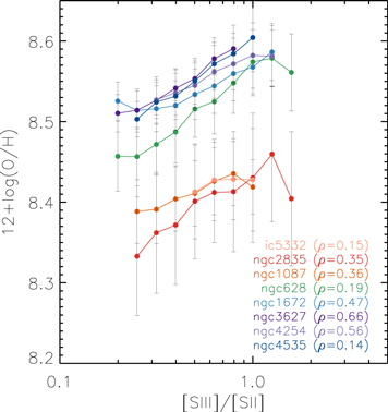
Figure 4. Metallicity of each H ii region as a function of the ionization parameter (as traced by [S iii]/[S ii]). Galaxies are color-coded by their total stellar mass from low (red) to high (blue) masses. The Spearman’s rank correlation coefficient (ρ) is listed for each, and all have high statistical significance (p < 0.001). All galaxies exhibit a positive correlation, with the offset between them set by the stellar mass–metallicity relation.
Download figure:
Standard image High-resolution imageThis positive correlation conflicts with theoretical predictions, which state that as stellar atmospheres of massive O stars become cooler with increasing metallicity there will be enhanced line and wind blanketing, resulting in a negative correlation (Massey et al. 2005). Most previous studies have found either negative correlations (Bresolin et al. 1999; Nagao et al. 2006) or no correlation (Kennicutt & Garnett 1996; Garnett et al. 1997; Dors et al. 2011; Poetrodjojo et al. 2018). However, they combined observations from different galaxies. Our analysis shows a clear trend within individual galaxies, which would be obscured when taken together if one studied only a few regions from each of several galaxies. A positive correlation has previously been observed in a sample of luminous infrared galaxies (LIRGs) (Dopita et al. 2014). These authors discuss this result mainly as a positive correlation between star formation rate surface density and ionization parameter, which they attribute to a difference in geometry. In this case, dense star-forming regions could contain inclusions of molecular clouds undergoing violent radiation pressure-dominated photoablation close to the exciting stars, resulting in a positive correlation between star formation surface density and ionization parameter. See Section 5.1 for further discussion on this.
To account for the metallicity offsets between galaxies introduced by the mass–metallicity relation, we subtract off the fitted radial metallicity gradients, and consider the residuals from the linear trend (ΔO/H, measured in logarithmic units). Apparent from our visualization of the metallicities across the galaxy disks (Figures 10–17) is the tendency for the more luminous (and more spatially extended) H ii regions to be more enriched. The left panel of Figure 5 traces this trend directly, demonstrating that ΔO/H increases systematically as a function of H ii region luminosity for all galaxies in our sample, with a Spearman’s rank correlation coefficient (ρ) of 0.34 and high statistical significance (p < 0.001). In total, we see a 0.03 dex increase in metallicity for the most luminous (LHα > 1038.5 erg s−1) regions.
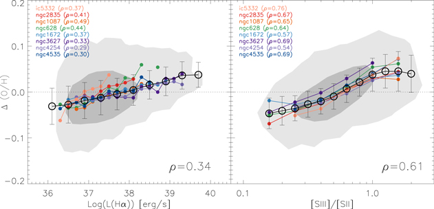
Figure 5. Trends in the metallicity offset from a radial gradient (ΔO/H) as a function of extinction-corrected Hα luminosity (left) and ionization parameter (as traced by [S iii]/[S ii], right). Galaxies are color-coded by their total stellar mass from low (red) to high (blue) masses. The median and 1σ scatter are overplotted in black. Background contours show the full distribution (98% and 68%). While we observe correlations with L(Hα), we observe the strongest systematic correlation with the [S iii]/[S ii] ratio, which is a tracer of the ionization parameter. The Spearman’s rank correlation coefficient (ρ; all with high statistical significance, p < 0.001) is calculated for each galaxy individually (top left) as well as for the sample as a whole (lower right).
Download figure:
Standard image High-resolution imageMoreover, we observe a much tighter correlation between ΔO/H and ionization parameter ([S iii]/[S ii]). We observe a stronger correlation (ρ = 0.63) for the sample as a whole, as well as improved correlation compared to the trends for individual galaxies between 12+log(O/H) and ionization parameter (Figure 4). This suggests the local physical conditions are very tightly linked to the localized enrichment of the ISM.
4.2. Physical Conditions of Regions with Enhanced and Reduced Abundances
We split the sample of H ii regions into those with (a) typical metallicities (−1σ < ΔO/H < 1σ), (b) enhanced metallicity (1σ < ΔO/H), and (c) reduced metallicity (ΔO/H < −1σ). In Figure 6 we show how the distributions of six physical parameters differ between the three samples. For all parameters explored, we find that the distribution of H ii regions with enriched/reduced metallicity is significantly different from the average sample. They show a Kolmogorov–Smirnov test probability value (p-value) less than 10–6, allowing us to reject the null hypothesis that the two samples are drawn from the same distribution.
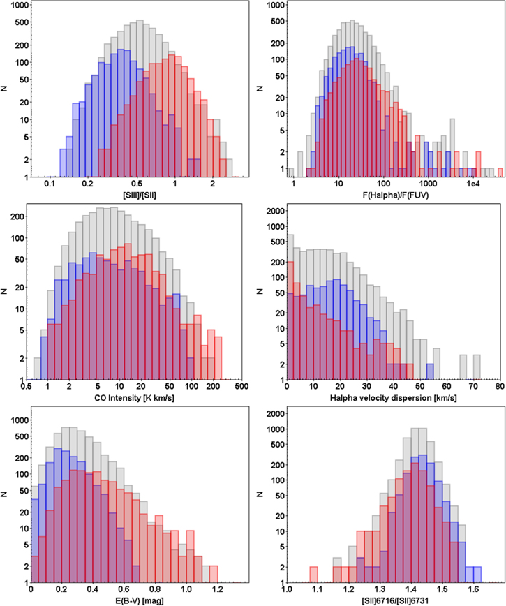
Figure 6. Distribution of six physical parameters of H ii regions with typical abundances (gray) as compared to H ii regions where the abundances are enhanced (ΔO/H > 1σ, red), or reduced (ΔO/H < −1σ, blue). All distributions are significantly different (Kolmogorov–Smirnov test p-value < 10–6). Compared to the depleted regions, enriched regions have markedly high [S iii]/[S ii] line ratios (indicating higher ionization parameter), as is also shown in Figure 5. They also have systematic offsets toward higher extinction corrected Hα-to-FUV flux ratio (indicating younger star cluster ages), higher CO intensity (indicating higher molecular gas densities), lower Hα velocity dispersions (indicating less mixing), higher  (indicating more dust along the line of sight), and lower [S ii]λ6716/[S ii]λ6731 line ratios (indicating higher electron densities).
Download figure:
Standard image High-resolution imageAs shown in Figure 5, the clearest correlation we see is with ionization parameter ([S iii]/[S ii]). As this traces the relative density of ionizing photons to the surrounding ISM gas density, we expect to find additional dependences on the stellar cluster age and on the local gas properties. In general, we expect H ii regions with younger, more massive star clusters and a denser surrounding medium to be characterized by higher ionization parameter values.
The Hα-to-FUV flux ratio has been shown to correlate with star cluster age (Sánchez-Gil et al. 2011), with younger clusters having larger flux ratios. We use GALEX imaging to measure the FUV flux at the position of each H ii region. In measuring the Hα flux we have convolved the Hα images to matched 45 resolution. We find that the H ii regions with enhanced metallicities tend toward higher extinction-corrected Hα-to-FUV flux ratios (younger star cluster ages). A similar trend is seen if we instead use the equivalent width of Hα as a tracer of star cluster age.
To probe the local ISM gas conditions, we use PHANGS–ALMA maps of the CO emission (Leroy et al. 2019) at 1″ spatial resolution to measure the local molecular gas surface density. While the angular resolution is well matched to our MUSE observations, this molecular material is necessarily not co-located with the ionized gas of the H ii region, and on our working ∼50 pc scales is likely associated with molecular clouds and associations neighboring the H ii regions (see also Kreckel et al. 2018), potentially representing the remnant of the cloud from which the H ii region formed (see Chevance et al. 2019; Kruijssen et al. 2019). We find that the H ii regions with enhanced abundances are at locations where we measure higher CO-integrated intensity, indicating a higher molecular gas surface density compared to the H ii regions with reduced abundances.
A change in the local ISM conditions is also seen when looking at the dust column along the line of sight (traced by the color excess,  ), which is generally thought to be well mixed with the gas. Here we find that the H ii regions with enhanced metallicities see higher dust columns along the line of sight, consistent with the previously described association with higher CO-integrated intensity, and implying higher gas surface densities. We note that this increased extinction is not enough to significantly bias our ability to detect enriched but low-luminosity H ii regions. Increased electron densities are also directly seen corresponding to the H ii regions with enhanced metallicity by comparing the density-sensitive line ratio [S ii]λ6716/[S ii]λ6731, though in most regions the ratio suggests electron densities at or below the low-density limit (<100 cm−3).
The velocity dispersion in the Hα line indicates the dynamical state of the ionized gas. In contrast to the H ii regions with enhanced abundances, the H ii regions with decreased abundances exhibit increased velocity dispersions (deconvolved from the instrumental resolution). This could indicate a difference in the large-scale mixing acting on the ISM, which would be needed to introduce less-enriched material. We also see a slight (2 km s−1) average increase in line width in the molecular gas phase for the most-enriched regions (not shown), suggestive of the ongoing impact of stellar feedback or association with more massive molecular clouds, but with less statistical significance (p-value of 0.002). This further suggests a (weak) local correlation between the Hα luminosity and the molecular gas line width.
To explore the spatial distribution of H ii regions with abnormal abundances, we show in an atlas (Appendix D, Figures 23–30) the azimuthal and spatial distribution of the metal offsets and the positions of these abnormal populations with respect to the ∼500 pc scale bulk CO emission (as measured by ALMA) of each galaxy. Here, our deliberate choice of low-resolution observations is designed to achieve high completeness in the integrated intensity. We use this CO map to trace the gas response to the underlying gravitational potential and other large-scale hydrodynamical effects.
While the azimuthal trends of H ii regions with reduced and enhanced abundances are discussed in more detail in the following section, we highlight here the difference between the spatial distribution of the two populations across the galaxy disks. Both populations are found across the full disks, but the H ii regions with reduced abundances are slightly more clustered in their distribution. Future work will explore in more detail the statistical properties of the H ii region metallicity distribution. Here we simply quantify this by calculating the average distance of the three nearest neighbors (n3) of all H ii regions with enhanced and reduced abundances. Computing this statistic using a larger number of neighbors shows similar trends but (naturally) larger clustering sizes. These trends are not dependent on the threshold we choose to separate the regions with enhanced and reduced abundances. As the enriched regions are only slightly larger on average in size than the total population (49 pc in radius compared to 45 pc), this cannot account for the systematic differences in clustering scale that we observe.

Figure 7. Clustering of the H ii regions with enhanced and reduced metallicities in relation to themselves (left) and in relation to the full H ii region population (right), as parameterized by the average distance to the three nearest neighbors (n3). The mean value for each galaxy is shown. We also normalize the right-hand figure to the clustering of the entire H ii region population across the whole galaxy. Galaxies are color-coded by their total stellar mass from low (red) to high (blue) masses. H ii regions with enhanced abundances relative to the radial gradient are systematically less clustered. IC 5332, our least massive and lowest star formation rate galaxy, shows less clustered star formation in general and a fairly flocculent morphology compared to the rest of the sample (Figure 17), but still shows an increase in clustering for the H ii regions with enhanced abundances.
Download figure:
Standard image High-resolution imageFigure 7 (left) shows a large scatter across this measure, but most galaxies show clustering on ∼300 pc scales of the reduced metallicity regions while enhanced metallicity regions are more widely distributed (n3 ∼ 400–600 pc; see also Figure 8). This suggests a connection between clustering and mixing, where isolated young regions with a history of star formation have the chance to become enriched (Ho et al. 2017, 2018). We further compare the clustering of the outliers in relation to the full H ii region population (Figure 7, right), relative to the average, and again find that the H ii regions with enhanced metallicities are less clustered.
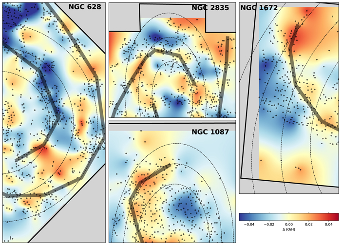
Figure 8. Zooming in on subsections of galaxies with the most pronounced azimuthal variations. Dashed ellipses in each galaxy mark fixed 1 kpc wide rings. The individual measurements of ΔO/H for each H ii region (circles) are interpolated onto a two-dimensional surface (shown in colorscale) using kriging and an exponential model. The brightest star-forming regions along the spiral arm have been traced by eye to provide a rough outline of the spiral pattern (overlaid in gray). Variations are seen in relation to the spiral arm in some cases (NGC 1672, NGC 1087) but more generally along fixed azimuth in other cases (NGC 628, NGC 2835). These variations are not perfectly symmetric, and are found in half of our sample.
Download figure:
Standard image High-resolution image4.3. Azimuthal Metallicity Variations
We find that the most enriched H ii regions are distributed across the disk, and simple statistical approaches where we try comparing changes in ΔO/H with large-scale environment (arm/interarm/bar), overdensities in stellar mass surface density, or dynamical tracers of the spiral pattern are inconclusive. For this paper, we simply present a few visualizations of how changes in ΔO/H are distributed spatially across the disk as an atlas in Appendix D (Figures 23–30). These images demonstrate the wealth of information we now have, but also the complicated nature of disentangling the preliminary azimuthal trends we see from their complicated environmental dynamics that vary widely between galaxies due to differences in their disk structure.
To match the metallicity maps presented in Appendix A, we similarly take our H ii region mask and paint on the measured ΔO/H corresponding to each H ii region. NGC 628, NGC 1087, NGC 1672, and NGC 2835 all show regular azimuthal variations at select rings. Such clear trends are not necessarily seen at all radii. NGC 3627 shows large-scale variations with much less regular patterns, but the remaining three galaxies show no obvious azimuthal trends. Subsections of the four galaxies showing the clearest signatures of azimuthal variations are highlighted in Figure 8. The morphology would suggest that this implies some correlation with the spiral structure, but when we compare the azimuthal metallicity variations with the total extinction-corrected Hα luminosity around the azimuthal ring (tracing the spiral structure), the connection is not so clear.
Enriched regions on the spiral arm often form a relatively narrow ridge, implying that the total count of such regions is not high (in contrast to high numbers in a thicker ridge). This may partially explain why it is not so easy to pick out trends when considering the population as a whole. This is particularly apparent in NGC 1087 and NGC 1672, but also to a lesser extent in NGC 628, NGC 2835, NGC 3627, and NGC 4535. The narrowness of this feature is in good agreement with the highly filamentary alignment of star-forming giant molecular clouds (GMCs) seen along spiral arms at high (∼50 pc) spatial resolution in nearby galaxies (Schinnerer et al. 2017; Kreckel et al. 2018; Kruijssen et al. 2019), and consistent with the association of the enriched regions with local conditions exhibiting high dust column and gas density (see Section 4.2). The regions with reduced abundances show a wider, more clustered distribution (see also Figure 7). They are often seen on the trailing side of the spiral arm (particularly on the eastern arm of NGC 1672). This is in very good agreement with the azimuthal variations identified by Ho et al. (2017, 2018).
In conclusion, we qualitatively identify half of our sample (NGC 628, NGC 1087, NGC 1672, and NGC 2835) as having azimuthal variations that are tenuously associated with the spiral pattern. The link to gas density can also be interpreted as indirect evidence for the influence of spiral arms, which tend to yield locally enhanced gas densities. Establishing more conclusively whether a correlation with the spiral pattern exists in a given galaxy will require an informed view of the dynamical structure specific to that disk.
5. Discussion
In this first look at a sample of galaxies with thousands of spatially isolated (<100 pc scale) H ii regions, we can begin to explore systematic trends and patterns in the abundance distributions.
5.1. Localized Enrichment within Galaxy Disks
We observe clear correlations between increased abundances relative to the radial trend (ΔO/H) and the local physical conditions of the ISM (Figures 5 and 6). The most fundamental positive correlation arises from changes in the ionization parameter (traced here by [S iii]/[S ii]), which tracks changes in the ionizing source, the ISM density, and H ii region geometry. Given how flat the radial ionization parameter gradient is (Figure 3), the high degree of correlation (Spearman’s rank correlation coefficient (ρ) of 0.60) between ΔO/H and [S iii]/[S ii] is quite striking.
Without removing the radial metallicity gradient, a trend between metallicity and ionization parameter is still apparent (Figure 4). Here, each galaxy appears offset in metallicity due to the well established relation between stellar mass and metallicity (Tremonti et al. 2004), and the correlation for any individual galaxy is weaker compared to the correlation within that galaxy when instead considering ΔO/H. Given that previous work generally has compared H ii region metallicities and ionization parameters by combining results from different galaxies with differing global metallicities (Bresolin et al. 1999; Dors et al. 2011), it is not surprising that the trends we now identify within individual galaxies would be washed out.
A similar positive correlation between metallicity and ionization parameter was reported in Dopita et al. (2014) for their analysis of resolved regions within 10 LIRGs. They observed similar trends between star formation rate and ionization parameter as well as between metallicity and ionization parameter, and argue that the trend arises as more active star-forming regions have a different distribution of molecular gas which favors higher ionization parameters. However, we are observing these trends within normal star-forming disk galaxies and, as we see in Figure 5, the observed trend is much weaker with the H ii region Hα luminosity, and the high-metallicity outliers are not more strongly clustered (Figure 7). Also, while we do see that the more enriched regions preferentially fall along the ridge of spiral arms in some regions of some galaxies, they are also found distributed throughout the disk, with no strong systematic trends with galaxy environment (see also Section 5.2). This suggests another explanation is required.
As we show in Figure 6, other local conditions correlate with the local changes in metallicity. Compared to the depleted regions, enriched regions have higher Hα-to-FUV flux ratios (indicating younger star cluster ages), higher  (indicating more dust along the line of sight), and lower [S ii]6716/[S ii]6731 line ratios (indicating larger electron densities). They also show higher CO intensity (indicating higher molecular gas surface densities) and slightly larger CO line widths (indicating kinematic disturbance in the local ISM). We note that the ISM conditions inferred from the CO are on matched angular scales (1″ ∼ 50 pc) but this material by nature does not co-exist with the ionized H ii region, so making a direct link between the physics occurring in these two different ISM phases is not straightforward. The trends, however, are very interesting, as they might represent two different evolutionary phases of the same underlying star-forming region even if they are somewhat spatially offset (e.g., Kruijssen et al. 2018).
As the H ii region metallicity generally reflects the ISM abundances locally before it was illuminated by the newest generation of stars, these trends are suggestive of a star formation history that has locally enriched the ISM. Recent work has suggested that star-forming complexes can host extended continuous star formation histories spanning ∼10 Myr (Rahner et al. 2018; Ramachandran et al. 2018). We see small systematic scatter in ΔO/H, and H ii regions with enhanced abundances typically show offsets of ∼0.05 dex. We perform a simple calculation to explore how much enrichment could be expected from a single generation of stars.
For a cloud of gas mass Mg = 5.8 × 10⁵ M⊙ (the typical GMC mass in NGC 628; Kreckel et al. 2018) and an integrated star formation efficiency per star formation event of = 0.05 (measured within the PHANGS sample; Chevance et al. 2019), this would produce
 M⊙ of new stars. Then, given an oxygen yield of yo = 0.00313 (based on observations; Kudritzki et al. 2015), when the massive stars die they return
  of oxygen to the surrounding ISM. Assuming perfect mixing within the cloud, this gives an upper limit on how much extra oxygen (by mass) can be added in one generation. Converting this to the change in oxygen abundance, this corresponds to an increase in log(O/H) of ∼0.02 dex with each generation of star formation. However, the oxygen yield is quite uncertain, and taking a theoretically motivated, higher oxygen yield of yo = 0.04 (Vincenzo et al. 2016) would result in an increase in log(O/H) of ∼0.18 dex. This demonstrates that the level of enrichment we report in this sample of eight galaxies is roughly consistent with what could be produced by a single generation of star formation.
We believe this is unlikely to be due to self-enrichment from a single burst of star formation, but could be consistent with an extended 5–10 Myr continuous star formation history. Typical supernova timescales (4 Myr; e.g., Leitherer et al. 2014) and subsequent mixing timescales over <100 pc scales (2 Myr; de Avillez & Mac Low 2002) are roughly equivalent to the expected H ii region lifetime (6–8 Myr; e.g., Kennicutt 1998; Chevance et al. 2019). Better constraints on the H ii region ages are needed to distinguish these scenarios. Simulations indicate that larger-scale (∼kpc) mixing is relatively inefficient (taking 100–350 Myr; Roy & Kunth 1995; de Avillez & Mac Low 2002), making it plausible that subsequent generations of stars could form before mixing has finished.
5.2. Subtle Evidence for Azimuthal Variations
In all galaxies we observe a very small systematic scatter (0.03–0.05 dex) after subtracting the radial gradients. This scatter is generally smaller than the amplitude of the radial variation, which typically ranges from 0.1 to 0.3 dex over the radial range we observe. It has been previously shown that strong line methods systematically produce smaller scatter in their radial gradients than direct temperature methods (Arellano-Córdova et al. 2016), but this very small systematic scatter with respect to the radial gradient is similar to what has been found using direct temperature methods to measure the metallicity in the Milky Way (Esteban & García-Rojas 2018). It is, however, much smaller than what has been found with direct temperature methods for three nearby galaxies by the CHAOS project (∼0.1 dex; Berg et al. 2015; Croxall et al. 2015, 2016) and in M33 (0.11 dex; Rosolowsky & Simon 2008).
We find azimuthal variations in half of the galaxies in our sample, but these trends are not always obviously associated with the spiral pattern. In all cases the azimuthal trends are more pronounced on only one spiral arm. In general, we find that H ii regions with enhanced or reduced metallicity are located across the full disk. Because of this, we have failed to distinguish any systematic correlations between changes in ΔO/H and environmental parameters (arm/interarm masks, stellar mass surface density offset). This suggests that, while the spiral pattern plays a role in organizing the ISM, it alone does not establish the azimuthal variations we observe, with changes also being driven by the strong correlations with the local physical conditions described in Section 5.1.
NGC 1672 presents a particularly interesting case (Figure 8), as the eastern arm shows a very clear ridge along the spiral arm with enhanced abundances. This appears very similar to the situation observed in the nearby galaxy NGC 1365 (Ho et al. 2017), with its widely separated spiral pattern, for which those authors proposed a carousel model where enrichment can proceed slowly in small pockets as gas passes through the interarm region, with enrichment peaking at the spiral arm. Passage through the spiral arm then triggers large-scale mixing, introducing more pristine gas from the surroundings and hence systematically decreasing the abundances. NGC 6754 (Sánchez-Menguiano et al. 2016) presents another case of azimuthal abundances attributed to the spiral pattern; however, in this case the drop in abundances is attributed to radial streaming motions that introduce more pristine gas to decrease the abundances, with trends differing on the leading and trailing sides of the arm.
The azimuthal variations reported here present a more complicated picture. Half of our eight galaxies show azimuthal variations, though often the case is much clearer across one half of the galaxy. NGC 1087 and NGC 1672 clearly show enhanced abundances along the spiral arm, but one is more flocculent while the other has a strong bar and a more pronounced spiral pattern. They also show different distributions for the enhanced regions, with NGC 1672 exhibiting a narrow (<100 pc) ridge while NGC 1087 has a broader (∼300 pc) enhanced region along the arm. NGC 628 and NGC 2835 show some regular azimuthal variations, but they do not correspond to the peaks in star formation. One significant difference between this study and previous work is our focus on the inner portions of the disk (R < 0.5 R25), whereas some recent theoretical work has suggested that azimuthal trends should be more pronounced in the outer disks near the corotation radius, where the relative velocity with respect to the pattern speed of the disk is close to zero (Spitoni et al. 2019).
Sánchez-Menguiano et al. (2019) carried out a detailed investigation of the local relation between star formation rate and metallicity, where for both quantities a radial relation has been removed. They find systematic trends that transition from a negative correlation at lower stellar masses to a positive correlation at higher stellar masses. While it is the case that the three most massive galaxies in our sample do not show azimuthal variations, the stellar masses for all galaxies in our sample do not range over more than an order of magnitude, so it is difficult to draw strong conclusions. Further progress could be made with more detailed dynamical models of each individual galaxy, but is beyond the scope of this paper.
5.3. Barred Galaxies with Flat Metallicity Gradients
Stellar bars drive gas inflows (Kormendy & Kennicutt 2004; Jogee et al. 2005), transporting metal-poor gas from the outer disk toward the galactic center. However, observations have presented conflicting evidence regarding whether or not barred spiral galaxies systematically exhibit flatter metallicity gradients (Vila-Costas & Edmunds 1992; Martin & Roy 1994; Zaritsky et al. 1994; Dutil & Roy 1999; Henry & Worthey 1999; Balser et al. 2011; Sánchez et al. 2014; Kaplan et al. 2016).
While an investigation of the connection between the metallicity gradients reported for this sample of eight galaxies and their morphological structure is beyond the scope of this work, flattened gradients are quite pronounced for three galaxies in our sample (NGC 1672, NGC 3627, and NGC 4535), particularly within the inner 0.1–0.3 R25 (Figure 2). All three of these show very strong stellar bars, which dominate the morphology over this inner radial range. NGC 3627 is also strongly interacting, and NGC 4535 is a member of the Virgo cluster. Three other galaxies in our sample are also classified as barred (NGC 1087, NGC 2835 and IC 5332; Table 1), exhibiting weaker stellar bars, and show no obvious flattening of their metallicity gradients. We draw no conclusions in this work, but find the connection between bar strength and flattened radial gradients intriguing.
5.4. Physical Interpretation of Line Ratios
We interpret the trends observed as changes in metallicity; however, in a practical sense what we are tracing are changes in the line ratios integrated across H ii regions. The physical interpretations of these line ratio diagnostics are not straightforward, with many showing degeneracies between changes in metallicity and ionization parameter, and are expected to then correlate with variations in star/cluster age, ISM density, and ISM pressure. Figure 9 explores how Levesque et al. (2010) photoionization models at fixed electron density (n = 100 cm−3) and ionization parameter (q = 2 × 10⁷) do produce variations in [S iii]/[S ii] as a function of both metallicity and stellar population age. Here we have taken the output line ratios from the “high” mass-loss tracks at three fixed metallicities (0.4 Z⊙, 1 Z⊙, and 2 Z⊙). Assuming an instantaneous burst of star formation, this age dependence can result in significant (factor of 3–5) changes in the predicted [S iii]/[S ii] line ratio. Taking models with a continuous star formation history results in almost no change in [S iii]/[S ii] with age.
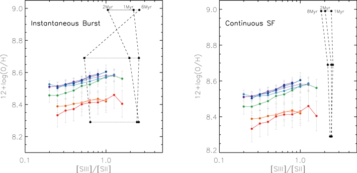
Figure 9. Comparison showing how changes in the age and metallicity of the stellar population are expected to affect the observed [S iii]/[S ii] line ratio for both an instantaneous burst (left) or continuous star formation history (right) at fixed ionization parameter. Here we show a grid from the Levesque et al. (2010) photionization models (n = 100 cm−3, q = 2 × 10⁷) over a range of ages (dashed lines) and metallicities (horizongal dotted lines; at fixed 0.4 Z⊙, 1 Z⊙, and 2 Z⊙, assuming a solar value of 12+log(O/H) = 8.69; Asplund et al. 2009) to demonstrate how the observed line ratios are expected to vary. This is overplotted on our observed relation (see also Figure 4). In the instantaneous burst models, age variations at fixed metallicity could theoretically account for some of the observed variation in [S iii]/[S ii]. In the continuous star formation models, very little change in [S iii]/[S ii] is expected at fixed metallicity (the dotted line is barely visible). Note that while the selected q value provides the best match to observations given the available models, it still does not cover well the observed range of [S iii]/[S ii].
Download figure:
Standard image High-resolution imageMore detailed photoionization and stellar population modeling, along with follow-up UV observations to constrain the stellar population age, are necessary to disentangle these effects. Shabani et al. (2018) found no dependence of star cluster age with distance to the spiral arm in two of the three nearby galaxies in their case study, including NGC 628, though their youngest age bin encompasses entirely this crucial 1–10 Myr regime. We note that the strong correlation between ΔO/H and [S iii]/[S ii] persists even if we attempt to clean our sample of some of these population extremes. Omitting regions with young ages (high Hα-to-FUV), high electron density (low [S ii]6716/[S ii]6731), high dust column (high  ), or close to the galaxy center does not fundamentally change the observed trend. More work is needed to explore fully the interconnection of these parameters and the impact each could have on the metallicity prescriptions.
An important final caveat to our discussion is that the trends we report are heavily dependent on the choice of metallicity prescription used. Appendix C explores this in more detail, but we emphasize here that our results are robustly reproduced if we instead use the Dopita et al. (2016) photoionization model-based N2S2 prescription. Given that this second prescription takes a very different approach compared to the empirical Pilyugin & Grebel (2016) prescription employed in this work, and should exhibit different biases, this builds further confidence in our results.
6. Conclusion
In the first results from the PHANGS–MUSE survey at ∼50 pc resolution we are able to cleanly separate individual H ii regions within our optical IFU data cubes and measure line fluxes from a spectrum integrated over individual H ii regions. By applying the Pilyugin & Grebel (2016) strong line prescription, we measure gas phase oxygen abundances for 7138 H ii regions across the disks of eight nearby galaxies. All galaxies are well fit by a simple linear metallicity gradient with small (0.03–0.05 dex) scatter.
Subtracting that radial trend, we compare physical parameters for those H ii regions that have enhanced and reduced abundances. Regions with enhanced abundances have high ionization parameter, higher Hα luminosity, younger star clusters, and associated molecular gas clouds show high CO line intesnity. This indicates that recent star formation, possibly the same that powers the H ii regions, has locally enriched the material. Regions with reduced abundances show increased Hα velocity dispersions, suggestive of mixing introducing more pristine material. We also identify a positive correlation between gas phase metallicity and ionization parameter, in conflict with theoretical predictions. Taken together, the trends we identify suggest the local physical conditions are tightly linked to the localized enrichment of the ISM.
We observe subtle evidence for systematic azimuthal variations in half of the sample, though often in only one half of the galaxy, and we cannot cleanly associate this with the spiral pattern in all cases. However, in NGC 1672 and NGC 1087 the strong correlations with spiral structure indicate that the spiral arms can play an important role in organizing and mixing the ISM. This presents a complicated picture of the interplay between galaxy dynamics and enrichment patterns, which we aim to more fully address in the future with the full PHANGS–MUSE sample.
We thank the referee for helpful comments that improved this work. K.K. gratefully acknowledges funding from the German Research Foundation (DFG) in the form of an Emmy Noether Research Group (grant No. KR4598/2-1, PI Kreckel). B.G. gratefully acknowledges the support of the Australian Research Council as the recipient of a Future Fellowship (FT140101202). F.S., E.S., C.F., P.L., RMcE, and T.S. acknowledges funding from the European Research Council (ERC) under the European Union’s Horizon 2020 research and innovation programme (grant agreement No. 694343). M.C. and J.M.D.K. gratefully acknowledge funding from the Deutsche Forschungsgemeinschaft (DFG) through an Emmy Noether Research Group (grant No. KR4801/1-1) and the DFG Sachbeihilfe (grant No. KR4801/2-1). J.M.D.K. gratefully acknowledges funding from the European Research Council (ERC) under the European Union’s Horizon 2020 research and innovation programme via the ERC Starting Grant MUSTANG (grant agreement No. 714907). E.R. acknowledges the support of the Natural Sciences and Engineering Research Council of Canada (NSERC), funding reference number RGPIN-2017-03987. S.C.O.G. acknowledges support from the DFG via SFB 881 “The Milky Way System” (sub-projects B1, B2 and B8) and also via Germany’s Excellence Strategy EXC-2181/1-390900948 (the Heidelberg STRUCTURES Excellence Cluster).J.P. and A.H. acknowledge funding from the Programme National “Physique et Chimie du Milieu Interstellaire” (PCMI) of CNRS/INSU with INC/INP, co-funded by CEA and CNES. F.B. acknowledge funding from the European Union’s Horizon 2020 research and innovation programme (grant agreement No. 726384).
This work is based on observations collected at the European Organisation for Astronomical Research in the Southern Hemisphere under ESO programme IDs 094.C-0623(A), 098.C-0484(A), 1100.B-0651(A) and 1100.B-0651(B).
This paper makes use of the following ALMA data: ADS/JAO.ALMA#2012.1.00650.S, ADS/JAO.ALMA#2015.1.00925.S, ADS/JAO.ALMA#2015.1.00956.S, ADS/JAO.ALMA#2017.1.00392.S,
ALMA is a partnership of ESO (representing its member states), NSF (USA) and NINS (Japan), together with NRC (Canada), MOST and ASIAA (Taiwan), and KASI (Republic of Korea), in cooperation with the Republic of Chile. The Joint ALMA Observatory is operated by ESO, AUI/NRAO and NAOJ. The National Radio Astronomy Observatory is a facility of the National Science Foundation operated under cooperative agreement by Associated Universities, Inc.
This work is based on observations made with the NASA Galaxy Evolution Explorer. GALEX is operated for NASA by the California Institute of Technology under NASA contract NAS5-98034.
The data analysis made use of Topcat (Taylor 2005). This research has made use of NASA’s Astrophysics Data System. This research has made use of the NASA/IPAC Extragalactic Database (NED), which is operated by the Jet Propulsion Laboratory, California Institute of Technology, under contract with the National Aeronautics and Space Administration.
Appendix A: Image Atlas
We present an atlas of images for each of the eight galaxies in our initial PHANGS–MUSE sample (Figures 10–17). All presented images are constructed from our MUSE data cubes, including the gri-band three-color images. For all galaxies, corresponding images are at matched image stretch and scaling. Each figure shows the gri-band three-color image (bottom left), overlaid emission line maps (red: Hα, green: [O iii], blue: [S ii]; bottom right), Hα emission (top left), and H ii regions with their measured metallicities (top right).
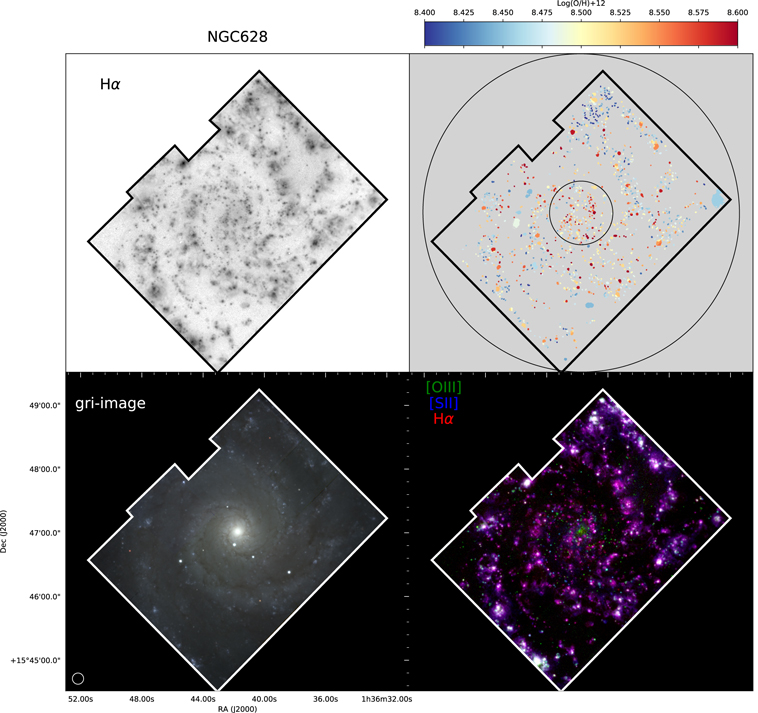
Figure 10. Mapping metallicity variations within the disks of NGC 628. Simulating a gri-band three-color image (bottom left) and overlaying emission line maps (red: Hα, green: [O iii], blue: [S ii]; bottom right) reveals the diversity of environments (bulge, spiral arms, dust lanes) and physical conditions across the disk. The Hα maps (top left) reveal a rich collection of H ii regions and diffuse ionized gas. Using H iiphot to identify H ii regions, we paint the H ii region mask with the measured metallicity (top right). Overlaid are ellipses at fixed 0.1 R25 and 0.5 R25. The circle in the lower left indicates a 500 pc diameter scale size; observations have a typical physical resolution of ∼50 pc (see also Table 1).
Download figure:
Standard image High-resolution image
Figure 11. Same as Figure 10, but for NGC 1087.
Download figure:
Standard image High-resolution image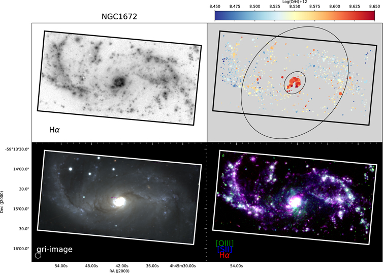
Figure 12. Same as Figure 10, but for NGC 1672.
Download figure:
Standard image High-resolution image
Figure 13. Same as Figure 10, but for NGC 2835.
Download figure:
Standard image High-resolution image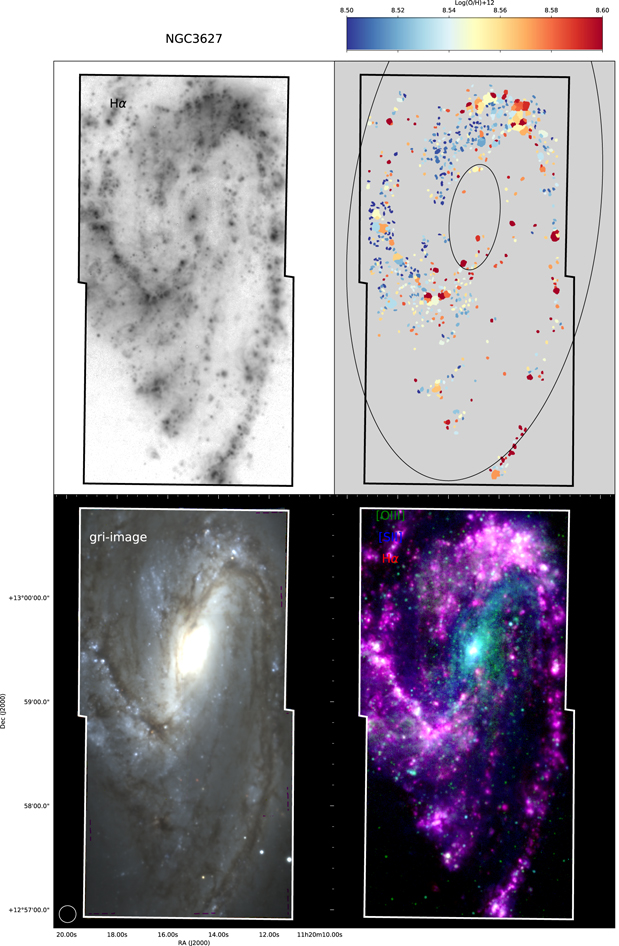
Figure 14. Same as Figure 10, but for NGC 3627.
Download figure:
Standard image High-resolution image
Figure 15. Same as Figure 10, but for NGC 4254.
Download figure:
Standard image High-resolution image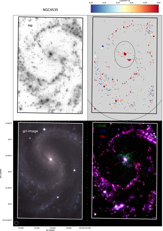
Figure 16. Same as Figure 10, but for NGC 4535.
Download figure:
Standard image High-resolution image
Figure 17. Same as Figure 10, but for IC 5332.
Download figure:
Standard image High-resolution imageAppendix B: Excitation Diagnostic Diagrams
We show BPT (Baldwin et al. 1981) diagnostic diagrams for all eight galaxies. In defining our H ii region catalog (Section 2.2), we employ two BPT emission line ratio diagnostics to ensure the excitation is consistent with photoionization by massive stars. In the [O iii]/Hβ versus [N ii]/Hα diagnostic (Figure 18), we require regions to be consistent with the stringent empirical Kauffmann et al. (2003) line. In the [O iii]/Hβ versus [S ii]/Hα diagnostic (Figure 19), we require regions to be consistent with the Kewley et al. (2001) line.

Figure 18. Diagnostic line ratios [O iii]/Hβ as a function of [N ii]/Hα (Baldwin et al. 1981) for all eight galaxies in our sample. H ii regions (black) populate a distributed but contained region in this parameter space. In gray are regions morphologically identified by H iiphot but that fail at least one of our selection criteria (see Section 2.2). Regions consistent with photoionization are expected to fall below the empirical Kauffmann et al. (2003) line (solid) and the theoretical Kewley et al. (2001) line (dotted). Median trends for each galaxy are plotted in the lower right panel, with galaxies color-coded by their stellar mass.
Download figure:
Standard image High-resolution image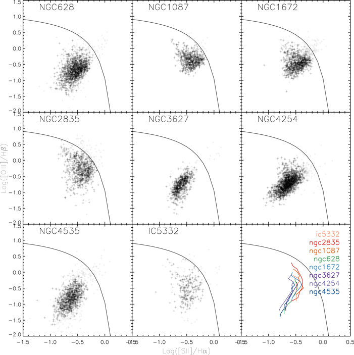
Figure 19. Diagnostic line ratios [O iii]/Hβ as a function of [S ii]/Hα (Baldwin et al. 1981) for all eight galaxies in our sample. H ii regions (black) populate a distributed but contained region in this parameter space. In gray are regions morphologically identified by H iiphot but that fail at least one of our selection criteria (see Section 2.2). Regions consistent with photoionization are expected to fall below the theoretical Kewley et al. (2001) line (solid). Median trends for each galaxy are plotted in the lower right panel, with galaxies color-coded by their stellar mass.
Download figure:
Standard image High-resolution imageEach diagram shows all regions morphologically identified by H iiphot, and in gray we indicate H ii regions that are excluded due to one of our rejection criteria listed in Section 2.2.
Appendix C: Metallicity Prescriptions
Strong line metallicity prescriptions produce well established differences in inferred metallicity and radial gradients in galaxies (Kewley & Ellison 2008; Poetrodjojo et al. 2019). In Figure 20 we present best-fitting radial metallicity gradients using four different prescriptions. This includes the Scal (solid lines; Pilyugin & Grebel 2016) prescription, which we have adopted in this work, as well as the Dopita et al. (2016) N2S2 (D16; dashed lines) photoionization model-based prescription, which gives qualitatively similar results. For completeness and to facilitate consistent comparisons with the exisiting literature, we also include the commonly used empirical Marino et al. (2013) O3N2 (dotted lines) and N2 (dashed–dotted lines) prescriptions. As in Section 3.2, each radial gradient is fit using all H ii regions with radius above  .
.
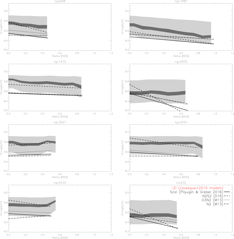
Figure 20. Fits to the radial metallicity gradients using four different prescriptions. We show here the Scal prescription (solid lines; Pilyugin & Grebel 2016), which we have assumed for this work, the Dopita et al. (2016) N2S2 photoionization model-based prescription (D16; dashed lines), and the commonly used empirical Marino et al. (2013) O3N2 (dotted lines) and N2 (dashed–dotted lines) prescriptions. Coefficients for each linear fit are given in Table 3. We overplot these on outputs from the Bayesian inference code IZI (Blanc et al. 2015), which derives the joint and marginalized posterior probability density functions (PDFs) for metallicity and ionization parameter. Here we have radially binned and summed the marginalized PDFs to produce a probabilistic metallicity gradient for each galaxy. Both the central 10% (dark gray) and 68% (light gray) percentile bands are shown.
Download figure:
Standard image High-resolution imageFinally, for further comparison with the results of photoionization models, we overplot each linear radial gradient on outputs from the Bayesian inference code IZI (Blanc et al. 2015). This code uses a set of observed line fluxes combined with an input photoionization model to derive the joint and marginalized posterior probability density functions for metallicity and ionization parameter. Here, we have compared all our observed strong emission lines ([O iii], Hβ, [N ii], Hα, [S ii], [S iii]) with the Levesque et al. (2010) “high” mass-loss tracks assuming a constant star formation history over the past 6 Myr and a Salpeter initial mass function with a 100 M⊙ upper cutoff. We then radially bin and sum the marginalized probability density functions to produce a probabilistic metallicity gradient for each galaxy. All gradients across all different methods show relatively good agreement in slope, and systematically ∼0.2 dex lower values in all empirical calibrations compared to the photoionization-based methods.
In Table 3 we list the coefficients of all radial gradient fits for each galaxies, using each of the four different metallicity prescriptions. R0 is the y-intercept, and the gradient is given both in units of R25 and in units of kpc. We further list the scatter with respect to the linear fit (σ(O/H)). Here, σ(O/H) reflects the standard deviation with respect to the linear radial gradient fit, whereas ΔO/H is the residual for a given point from the fit. This scatter is systematically lower (∼0.04 dex) in all empirical calibrations (Scal, O3N2, N2) compared to the N2S2 (D16) photoionization model-based calibration (∼0.09 dex).
While the radial gradients appear quite consistent across calibrations, and the scatter σ(O/H) is also similar between empirical calibrations, the different calibrations show very different trends between ΔO/H and L(Hα) and [S iii]/[S ii] (a proxy for the ionization parameter). In Figure 21 we show this trend using each of the four prescriptions for each galaxy individually and for the entire sample. Both the Scal and N2S2 (D16) calibrations exhibit a positive correlation with both L(Hα) and [S iii]/[S ii] that is discussed in this paper. On the other hand, O3N2 and N2 show a quite flat trend. However, because these are both using smaller dimensionallity in the line ratios, we believe both of these presciptions retain some of the degeneracy between metallicity and ionization parameter, enough to cloud the subtle trends presented here.

Figure 21. Trends between ΔO/H and L(Hα) (top) and [S iii]/[S ii] (bottom; a proxy for the ionization parameter) for four different metallicity prescriptions. The Scal (adopted throughout this paper) and N2S2 (D16) prescriptions show positive correlations, with the ionization parameter exhibiting a more fundamental correlation. O3N2 (M13) and N2 (M13) show no trend with either parameter. Different galaxies are represented by different colors as in Figure 18.
Download figure:
Standard image High-resolution imageA final demonstration of the strong discrepancies between calibrations is shown in Figure 22. Here, we calculate ΔO/H for the same H ii regions using different prescriptions, and compare the 1σ outliers. Between the Scal and N2S2 (D16) calibrations we find a clear correlation, with 50%–60% of outliers overlapping between the two calibrations. N2 (M13) shows poor agreement with Scal, with only ∼20% of the outliers agreeing between the samples. O3N2 shows no correlation with Scal, having <10% of the outliers overlapping. While both O3N2 and N2 quantitatively reproduce the radial metallicity gradient slope, they appear to be insensitive to much of the small-scale physics related to small metallicity variations recovered by both the Scal and N2S2 (D16).
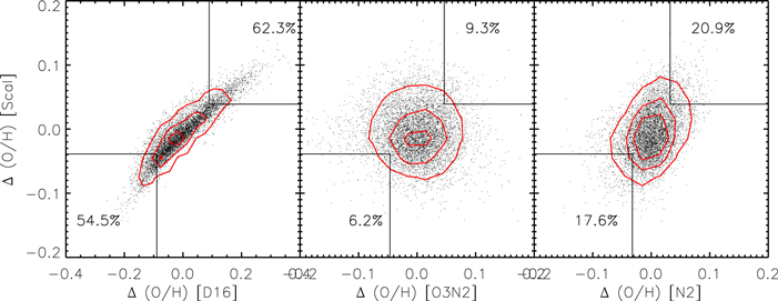
Figure 22. For the same H ii regions, we compute ΔO/H using different metallicity prescriptions in order to compare the overlap of the outlier populations. Each plot marks with boxes the 1σ outliers in each calibration, with the fraction of outliers overlapping between samples given in each box. Scal and N2S2 (D16, left) show good agreement, with 50%–60% of 1σ outliers agreeing between the two prescriptions. N2 (M13, right) shows poor agreement (∼20%), and O3N2 (M13, center) shows no correlation (<10% agreement in outliers).
Download figure:
Standard image High-resolution image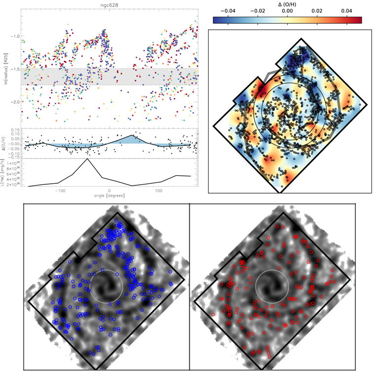
Figure 23. Visualizing the azimuthal variations within NGC 628. Top left: we unwrap the spiral structure into a polar projection, plotting the azimuthal angle on the x-axis and the natural log of the radius on the y-axis. We indicate each H ii region as a dot (removing any biases from size or luminosity) color-coded by ΔO/H. We choose one ring at fixed deprojected radius that best exemplifies azimuthal variations in ΔO/H and how it relates to the azimuthal Hα extinction-corrected luminosity. These rings are 0.1 R25 wide, and selected to be completely contained within the mask but demonstrating the strongest trend for azimuthal variations. To guide the eye, we overplot the median ΔO/H measured in 30◦ wide bins, and color the positive and negative residuals with respect to ΔO/H = 0 (top left, middle panel). We compare this with the total extinction-corrected luminosity around the same azimuthal ring in matched 30◦ wide bins (top left, bottom panel). Top right: the individual measurements of ΔO/H for each H ii region (circles) are interpolated onto a two-dimensional surface using kriging and an exponential model. We mark an approximate spiral arm location by tracing the brightest star-forming regions along the arm by eye (overlaid in gray). The same ring at fixed deprojected radius is also drawn. Bottom: we overlay the positions of all regions with enhanced (red) or reduced (blue) abundances onto an image of the bulk CO emission to highlight their position in relation to the spiral structure. NGC 628 shows tentative evidence for azimuthal variations; however, in the ring at fixed deprojected radius it appears the enhancement is anti-correlated with the spiral pattern. Results for the remaining galaxies are shown in the following figures. We tentatively identify azimuthal variations in half the galaxies shown, though a correlation with spiral structure is not always clear.
Download figure:
Standard image High-resolution image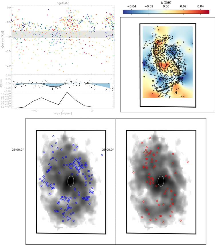
Figure 24. Visualizing the azimuthal variations within NGC 1087, as described in Figure 23. NGC 1087 shows clear systematic enhancement broadly spread across the northern spiral arm. Such a trend is much less obvious on the southern arm, though hinted at in the ring at fixed deprojected radius.
Download figure:
Standard image High-resolution image
Figure 25. Visualizing the azimuthal variations within NGC 1672, as described in Figure 23. NGC 1672 shows clear systematic enhancement along a narrow ridge in the eastern spiral arm. No similar trend is seen on the western arm, though the spiral pattern is also less pronounced.
Download figure:
Standard image High-resolution image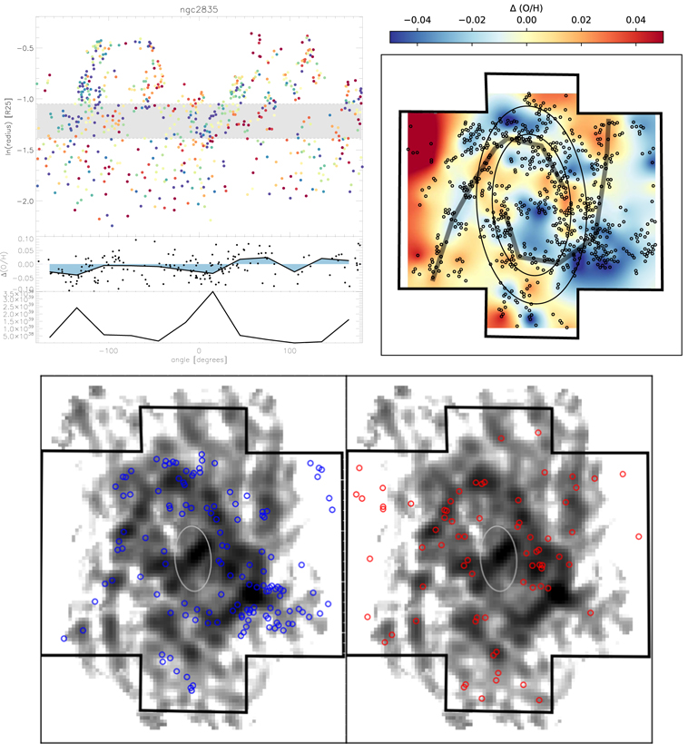
Figure 26. Visualizing the azimuthal variations within NGC 2835, as described in Figure 23. NGC 2835 shows azimuthal variations along the ring at fixed deprojected radius with enhanced abundances that are anti-correlated with the spiral structure. Some general preference of the enhanced regions to sit along the spiral pattern is, however, seen in the bottom two panels.
Download figure:
Standard image High-resolution image
Figure 27. Visualizing the azimuthal variations within NGC 3627, as described in Figure 23. NGC 3627 does not show any clear azimuthal variation, and our field of view is morphologically dominated by the stellar bar and strongly star-forming bar-ends.
Download figure:
Standard image High-resolution image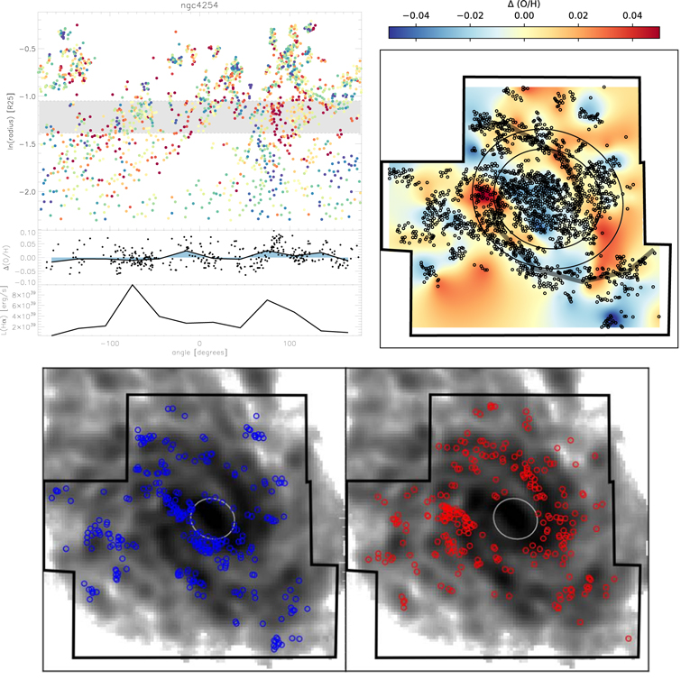
Figure 28. Visualizing the azimuthal variations within NGC 4254, as described in Figure 23. NGC 4254 exhibits a very flocculent spiral pattern, and does not show any clear azimuthal variation.
Download figure:
Standard image High-resolution image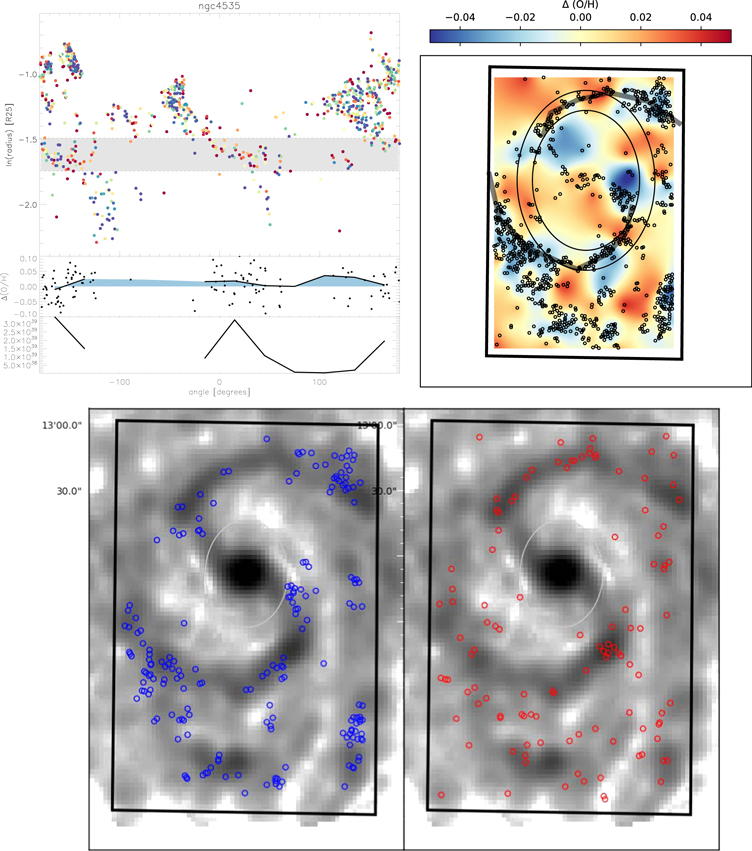
Figure 29. Visualizing the azimuthal variations within NGC 4535, as described in Figure 23. NGC 4535 has a well defined spiral pattern and does not show any clear azimuthal variation. It does have a ridge of enhanced regions along the northern spiral arm.
Download figure:
Standard image High-resolution image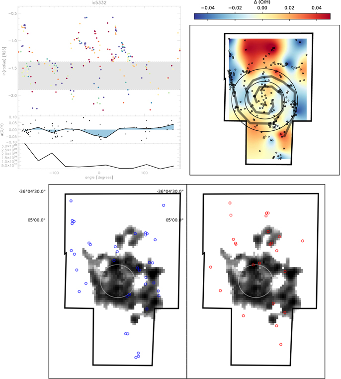
Figure 30. Visualizing the azimuthal variations within IC 5332, as described in Figure 23. This flocculent galaxy has very little CO emission, though our ALMA coverage is well matched to the MUSE field of view. IC 5332 has a tightly wound spiral pattern and low star formation rate, and does not show any clear azimuthal variation.
Download figure:
Standard image High-resolution imageAppendix D: Azimuthal Variations Atlas
For each galaxy, we present two visualizations of the complete spatial distribution of ΔO/H (Figures 23–30). Removing any size or luminosity information, we take the position of each H ii region and place it onto a polar projection, with the azimuthal angle on the x-axis and the natural log of the radius on the y-axis (upper left panels). Here we color-code each region by ΔO/H. In polar plots, spiral arms with fixed pitch angle appear as straight lines. As an alternative visualization (upper right panels), we also take the individual measurements of ΔO/H for each H ii region (circles) and interpolate them onto a two-dimensional surface using kriging and an exponential model. We mark an approximate spiral arm location by tracing the brightest star-forming regions along the arm by eye (overlaid in gray), though we note here this is very approximate and not sufficient for detailed environmental comparisons.
We mark in each of these images a ring at fixed radius, matched between both images, and show below the polar plot how ΔO/H varies azimuthally. These rings are  wide, and selected to be completely contained within the mask but demonstrating the strongest trend for azimuthal variations. To guide the eye, we overplot the median ΔO/H measured in 30◦ wide bins, and color the positive and negative residuals with respect to ΔO/H = 0 (top left, middle panel). We compare this with the total extinction-corrected luminosity around the same azimuthal ring in matched 30◦ wide bins (top left, bottom panel).
As a final visualization, we also map the locations of the H ii regions that are 1σ outliers toward both enhanced and reduced abundances (bottom panels). We show these populations in relation to the ∼500 pc scale bulk CO emission, roughly tracing the underlying gravitation potential and the spiral pattern.
Discussion of the trends identified within each galaxy and across the galaxy sample is contained in Sections 4.3 and 5.2.