Abstract
We found a simultaneous decrease of the Fe–K line and 4.2–6 keV continuum of Cassiopeia A with the monitoring data taken by the Chandra X-ray Observatory in 2000–2013. The flux change rates in the whole remnant are −0.65 ± 0.02% yr−1 in the 4.2–6.0 keV continuum and −0.6 ± 0.1% yr−1 in the Fe–K line. In the eastern region where the thermal emission is considered to dominate, the variations show the largest values: −1.03 ± 0.05% yr−1 (4.2–6 keV band) and −0.6 ± 0.1% yr−1 (Fe–K line). In this region, the time evolution of the emission measure and the temperature have a decreasing trend. This could be interpreted as adiabatic cooling with the expansion of m = 0.66. On the other hand, in the non-thermal emission dominated regions, variations of the 4.2–6 keV continuum show smaller rates: −0.60 ± 0.04% yr−1 in the southwestern region, −0.46 ± 0.05% yr−1 in the inner region, and +0.00 ± 0.07% yr−1 in the forward shock region. In particular, flux does not show significant change in the forward shock region. These results imply that strong braking in shock velocity has not been occurring in Cassiopeia A (<5 km s−1 yr−1). All of our results support the idea that X-ray flux decay in the remnant is mainly caused by thermal components.
1. Introduction
Supernova remnants (SNRs) are known to be one of the most dynamic phenomena in the universe. Spectral and image evolutions are quicker when the age of the remnants are younger, since the shock velocity is faster and its braking is larger. Recently, there have been several hypotheses about X-ray spectral variations from young SNRs (e.g., Uchiyama et al. 2009; Uchiyama & Aharonian 2008; Patnaude et al. 2011). Mainly, the variable component is considered to be synchrotron X-rays (non-thermal X-rays) caused by high-energy electrons in the amplified magnetic field (∼mG). Also, time series of images revealed moments of expanding shell structures in young SNRs (e.g., Fesen et al. 2006; Katsuda et al. 2008; Patnaude & Fesen 2009). These facts tell us that SNRs are experiencing an extreme evolution, and we can detect these evolutions in our observational timescale (∼10 year). Such information would be very useful for understanding how the remnants evolve and affect the ambient medium.
Cassiopeia A, a Galactic young remnant ∼340 years old (Fesen et al. 2006), has been found to display several X-ray time variations by intensive observations with the Chandra X-ray Observatory. Patnaude & Fesen (2007) found year-scale X-ray variability in thermal and non-thermal knots using the Chandra data taken in 2000, 2002, and 2004. In the entire face of the remnant, they identified six time-varying structures, four of which show a count rate increase from ∼10% to over 90%. Uchiyama & Aharonian (2008) analyzed the same data set and found year-scale time variation in the X-ray intensity for a number of non-thermal X-ray filaments or knots associated with reverse-shocked regions. They found that variable non-thermal features prevail over thermal ones. Patnaude et al. (2011) found a steady ∼1.5%–2% yr−1 decline in the 4.2–6.0 keV band of the overall X-ray emission of Cassiopeia A. They discussed a possible cause of this decline as a deceleration of the forward shock velocity. Strong braking ≈30–70 km s−1 yr−1 was necessary to explain the decay of the X-ray flux.
On the other hand, we cannot completely ignore a thermal X-ray contribution to the time evolution because the continuum emissions below 4 keV not have only a non-thermal component but also a thermal bremsstrahlung component. Helder & Vink (2008) estimated that the fraction of non-thermal component is ∼54% in the 4.2–6 keV band. No significant X-ray variability in the soft X-ray band (1–3 keV) has been found (e.g., Patnaude et al. 2011; Rutherford et al. 2013). However, we note the possibility that the 4.2–6 keV and 1–3 keV band emissions may originate from different plasma. The spectrum of Cassiopeia A can be well fitted with a two temperature thermal model (e.g., Willingale et al. 2002; Hwang & Laming 2009) in addition to the non-thermal component. Of the two thermal components, the higher temperature one occupies a significant fraction of the observed 4.2–6 keV spectrum, and explains the entire Fe–K line. In addition, iron spatial distribution in Cassiopeia A is not similar to the hard X-ray intensity distribution (e.g., Grefenstette et al. 2015). The thermal component has a different spatial distribution from the non-thermal component, and hence we believe it is worth investigating the time variation of the thermal component.
In this paper, while maintaining the possibility of time variation of the thermal component, we aim to identify the variable component of the 4.2–6 keV band of Cassiopeia A in more detail. We investigate time variations in the 4.2–7.3 keV band including the Fe–K emission lines by using Chandra ACIS for the first time. Time variations in thermal emission dominated and non-thermal emission dominated regions are also investigated.
2. Observation and Data Reduction
2.1. Chandra ACIS-S
For our study of the year-scale variability in flux, data from the Chandra X-ray Observatory were utilized. Chandra observations of Cassiopeia A have been carried out several times since launch in 1999 (e.g., Hwang et al. 2000, 2004; Patnaude et al. 2011; Hwang & Laming 2012; Patnaude & Fesen 2014). The data used in our analysis are listed in Table 1. Archived data taken with ACIS-S in Timed Exposure mode are gathered. ACIS-S3 is a back-illuminated CCD chip with enhanced soft X-ray response and fairly constant spectral resolution during the course of the mission compared to the ACIS-I array. The satellite and instrument are described by Weisskopf et al. (2002).
Table 1. Chandra Observation Log
| ObsID. | Date | Exposure (ks) | SI Mode |
|---|---|---|---|
| YYYY MM DD | |||
| 114 | 2000 Jan 30 | 49.9 | TE_002A0 |
| 1952 | 2002 Feb 06 | 49.6 | TE_002A0 |
| 5196 | 2004 Feb 08 | 50.2 | TE_002A0 |
| 5319 | 2004 Apr 18 | 42.3 | TE_003DA |
| 9117 | 2007 Dec 05 | 24.8 | TE_003DA |
| 9773 | 2007 Dec 08 | 24.8 | TE_003DA |
| 10935 | 2009 Nov 02 | 23.3 | TE_009E2 |
| 12020 | 2009 Nov 03 | 22.4 | TE_009E2 |
| 10936 | 2010 Oct 31 | 32.2 | TE_009E2 |
| 13177 | 2010 Nov 02 | 17.2 | TE_009E2 |
| 14229 | 2012 May 15 | 49.1 | TE_009E2 |
| 14480 | 2013 May 20 | 48.8 | TE_009E2 |
Download table as: ASCIITypeset image
We reprocessed the event files (from level 1 to level 2) to remove pixel randomization and to correct for CCD charge transfer efficiencies using CIAO version 4.6 and CalDB 4.6.3. Bad grades were filtered out and good time intervals were reserved. Cassiopeia A is so bright that the data were all taken with the single chip operation mode of S3 to avoid telemetry loss. Cassiopeia A was usually pointed near the center of the ACIS-S3 chip of 1024 × 1024 pixel CCDs, each with 05 × 0
5 pixels and a field of view of 8
4 × 8
4. The pointing position was moderately shifted from the aim-point and its roll angle varied from observation to observation. The effective areas (arf) of individual observations were then calculated for each ObsID using the Chandra standard analysis software package mkwarf in CIAO.
2.2. Suzaku XIS0 & XIS3
For tracing the non-thermal emission, Suzaku data were utilized. A deep observation with Suzaku was made in 2012. The exposure time was 205 ksec long (XIS0+XIS3). Suzaku has four X-ray CCD cameras (XIS: Koyama et al. 2007; Uchiyama et al. 2007). One of the four XIS detectors (XIS 1) is back-side illuminated (BI) and the other three (XIS 0, XIS 2, and XIS 3) are front side illuminated (FI). In the XIS data taken with the Spaced-row Charge Injection option in normal exposure mode, gap columns due to injected charges appear every 54 lines. The column widths of the FIs are three pixels which are smaller than five for the BI. To minimize flux uncertainty due to the gap, we used only FI data. In the FI CCDs, XIS-2 was not operational in 2012. Data screening was made with standard criteria provided by the Suzaku processing team.
3. Analysis and Results
3.1. Region Selection
X-ray emissions from Cassiopeia A are known to be a composite of thermal and non-thermal components (e.g., Hughes et al. 2000). The thermal component is characterized by emission lines from highly ionized ions of heavy elements such as iron, accompanied with a continuum emission by a thermal bremsstrahlung. The non-thermal emission is known to be traced by a hard band continuum emission above 10 keV (e.g., Maeda et al. 2009). Figure 1 shows a hard X-ray image (10–12 keV band) with Suzaku. We can see the concentrated hard X-ray distribution from the western region toward the center of Cassiopeia A. Figure 2 shows three color images from Chandra in the 4.2–6.0 keV, the 6.54–6.92 keV (Fe–K line), and the 1.75–1.95 keV (Si–K line) bands overlaid with the Suzaku contour in the 10–12 keV band. The Fe–K emission is believed to originate from optically thin thermal plasma. Using the Suzaku contour map and the Chandra lines, we can segregate the distributions of the thermal and non-thermal X-rays. Based on this information, five local regions and one whole SNR region were selected from the image for our analysis.
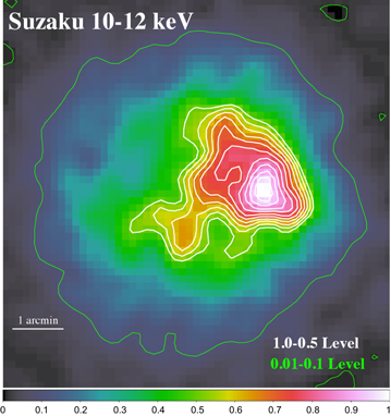
Figure 1. Suzaku XIS image corrected for the exposure map (i.e., the vignetting function of the telescope) in the 10–12 keV band. This image was binned by 8 × 8 pixels, and was then smoothed with a Gaussian function with a sigma of 3 bins (=0.42 arcmin). The image is normalized by the value of the pixel value of the maximum brightness. White and green contours show the range of 1.0(maximum brightness)–0.5 and 0.1–0.01, respectively.
Download figure:
Standard image High-resolution image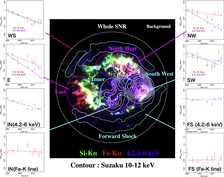
Figure 2. Three color images of Cassiopeia A with Chandra overlaid with a Suzaku contour in the 10–12 keV band. Blue, red, and green colors show the 4.2–6.0 keV, 6.54–6.92 keV (Fe–K line), and 1.75–1.95 keV (Si–K line) band images, respectively. Each plot around the image shows the time evolution of observed flux of Cassiopeia A at each region (whole SNR: WS, east: E, inner: I, north west: NW, south west: SW, forward shock: FS). Blue and red data show flux of the 4.2–6 keV band and Fe–K line normalized at the first data point, respectively. Solid lines show best-fit linear models. The error bars of all figures are 1σ.
Download figure:
Standard image High-resolution imageWe defined the “east” and the “north west” regions as the “thermal dominant” region (magenta ellipses in Figure 2). The east region has the most abundant X-ray flux of the Fe–K line. Therefore, this region is the best region to discuss the time evolution of the Fe–K line with less of a non-thermal emission contribution. The north west region is the second luminous region of the Fe–K line emission. This region shows a separation from the hard X-ray peak and a separation from continuum X-ray dominant region (DeLaney et al. 2004; Helder & Vink 2008).
On the other hand, we defined “south west,” “inner”, and “forward shock” regions as the “non-thermal dominant” region (light blue regions in Figure 2). Helder & Vink (2008) and DeLaney et al. (2004) show the area dominated by a harder spectrum. As a matter of fact, these regions manifest themselves in hard X-rays. Our image also shows the inner region is bright with hard X-rays. In addition, the forward shock has a featureless non-thermal emission (e.g., Hughes et al. 2000; Bamba et al. 2005). In the forward shock, it was found that the average proper motion of Cassiopeia A is 030 yr−1 (Patnaude & Fesen 2009), so we corrected the forward shock region of each year with this value (see the
3.2. Spectra
With the regions defined in the Section 3.1, we extracted spectra using a custom pipeline based on specextract in CIAO script. Here, the background spectra were extracted from outside of the whole SNR region defined in Figure 2. Since X-ray emission from Cassiopeia A is very strong, the background contribution is almost negligible for a time variation estimation. The background fraction of the whole SNR is only ∼3% in the 4.2–7.3 keV band and this is almost constant value from 2002 to 2013. In 2000, this fraction shows a larger value (∼7%) presumably because of an increase in the charged particle flux experienced during this observation. After background subtraction, we fitted the 4.2–7.3 keV band spectra at each epoch with a power-law model and a Gaussian line with XSPEC version 12.8.2. The best-fit parameters are summarized in Table 2.
Table 2. Best-fit Parameters of the ACIS Spectraa
| Epoch | Power-law Model | Fe–K Line | χ2/d.o.f | ||||
|---|---|---|---|---|---|---|---|
| Γ | Flux (4.2–6 keV) | Energy | EW | Flux | |||
| (Year) | (×10−11 erg cm−2 s−1) | (keV) | (keV) | (×10−3 ph cm−2 s−2) | |||
| Whole SNR | |||||||
| 2000.1 | 2.90 ± 0.02 |

|

|
0.95 ± 0.01 | 5.27 ± 0.05 | 347.52/206 | |
| 2002.1 | 2.99 ± 0.02 | 17.39 ± 0.03 |

|
1.00 ± 0.01 | 5.22 ± 0.04 | 322.02/206 | |
| 2004.1 | 2.99 ± 0.01 |

|

|
0.98 ± 0.01 | 5.12 ± 0.03 | 355.18/206 | |
| 2007.9 | 3.00 ± 0.02 | 16.52 ± 0.03 | 6.6377 ± 0.001 | 1.02 ± 0.01 | 5.05 ± 0.04 | 324.81/206 | |
| 2009.8 | 3.00 ± 0.02 | 16.21 ± 0.03 |

|
0.99 ± 0.01 | 4.79 ± 0.04 | 321.93/206 | |
| 2010.8 | 2.99 ± 0.02 | 16.48 ± 0.03 |

|
0.97 ± 0.01 | 4.83 ± 0.04 | 322.59/206 | |
| 2012.4 | 2.95 ± 0.02 | 16.44 ± 0.03 | 6.6503 ± 0.001 | 1.00 ± 0.01 | 4.97 ± 0.04 | 278.20/206 | |
| 2013.4 | 3.00 ± 0.02 | 16.31 ± 0.03 | 6.6419 ± 0.001 | 1.01 ± 0.01 | 4.93 ± 0.04 | 268.78/206 | |
| East | |||||||
| 2000.1 | 3.22 ± 0.04 | 2.52 ± 0.01 | 6.677
|
2.53 ± 0.03 | 1.77 ± 0.02 | 291.35/206 | |
| 2002.1 | 3.31 ± 0.04 | 2.45 ± 0.01 | 6.675
|
2.67
|
1.76 ± 0.02 | 307.28/206 | |
| 2004.1 | 3.29 ± 0.03 | 2.37 ± 0.01 | 6.685 ± 0.002 | 2.66
|
1.70 ± 0.01 | 420.74/206 | |
| 2007.9 | 3.30 ± 0.04 | 2.32 ± 0.01 | 6.677
|
2.79
|
1.75 ± 0.02 | 299.12/206 | |
| 2009.8 | 3.31 ± 0.04 | 2.26 ± 0.01 | 6.679
|
2.76 ± 0.04 | 1.68 ± 0.02 | 278.59/206 | |
| 2010.8 | 3.28 ± 0.04 | 2.28 ± 0.01 | 6.672
|
2.71
|
1.68 ± 0.02 | 270.84/206 | |
| 2012.4 | 3.30 ± 0.05 | 2.17 ± 0.01 | 6.711
|
2.82
|
1.62 ± 0.02 | 307.66/206 | |
| 2013.4 | 3.40 ± 0.05 | 2.15 ± 0.01 | 6.704
|
2.89
|
1.61 ± 0.02 | 292.35/206 | |
| North West | |||||||
| 2000.1 | 2.98 ± 0.03 | 3.73
|
6.584
|
1.61 ± 0.02 | 1.85 ± 0.02 | 316.05/206 | |
| 2002.1 | 3.03 ± 0.03 | 3.66 ± 0.01 | 6.589
|
1.66 ± 0.02 | 1.85 ± 0.02 | 283.29/206 | |
| 2004.1 | 3.06 ± 0.02 | 3.63 ± 0.01 | 6.597 ± 0.001 | 1.67 ± 0.02 | 1.83 ± 0.02 | 389.43/206 | |
| 2007.9 | 3.12 ± 0.03 | 3.44 ± 0.01 | 6.596
|
1.74
|
1.78 ± 0.02 | 277.33/206 | |
| 2009.8 | 3.15 ± 0.04 | 3.26
|
6.605
|
1.83 ± 0.03 | 1.75 ± 0.02 | 287.39/206 | |
| 2010.8 | 3.17 ± 0.04 | 3.34 ± 0.01 | 6.597
|
1.86 ± 0.03 | 1.81 ± 0.02 | 232.13/206 | |
| 2012.4 | 3.01 ± 0.03 | 3.39 ± 0.01 | 6.618
|
1.78 ± 0.02 | 1.83 ± 0.02 | 267.84/206 | |
| 2013.4 | 3.04 ± 0.03 | 3.28
|
6.604
|
1.82 ± 0.02 | 1.80 ± 0.02 | 290.10/206 | |
| South West | |||||||
| 2000.1 | 2.74 ± 0.03 | 3.92
|
6.614
|
0.60 ± 0.01 | 0.77 ± 0.02 | 242.97/206 | |
| 2002.1 | 2.83 ± 0.03 | 3.90 ± 0.01 | 6.623
|
0.62
|
0.76 ± 0.02 | 214.20/206 | |
| 2004.1 | 2.78 ± 0.02 | 3.94 ± 0.01 | 6.630 ± 0.002 | 0.59 ± 0.01 | 0.75 ± 0.01 | 229.44/206 | |
| 2007.9 | 2.82 ± 0.03 | 3.65
|
6.627 ± 0.003 | 0.62 ± 0.02 | 0.72 ± 0.02 | 265.07/206 | |
| 2009.8 | 2.82 ± 0.03 | 3.61
|
6.631 ± 0.003 | 0.62 ± 0.02 | 0.71 ± 0.02 | 220.24/206 | |
| 2010.8 | 2.80 ± 0.03 | 3.63 ± 0.01 | 6.627
|
0.62
|
0.73 ± 0.02 | 265.88/206 | |
| 2012.4 | 2.80 ± 0.04 | 3.75 ± 0.01 | 6.636
|
0.66 ± 0.02 | 0.78 ± 0.03 | 230.55/206 | |
| 2013.4 | 2.82 ± 0.03 | 3.71 ± 0.01 | 6.629
|
0.64 ± 0.02 | 0.75 ± 0.02 | 264.19/206 | |
| Forward Shock | |||||||
| 2000.1 | 2.55 ± 0.06 | 1.57 ± 0.01 | 6.63
|
0.22 ± 0.02 | 0.12 ± 0.02 | 198.16/206 | |
| 2002.1 | 2.64 ± 0.05 | 1.562
|
6.61
|
0.18 ± 0.02 | 0.10 ± 0.01 | 208.52/206 | |
| 2004.1 | 2.69 ± 0.04 | 1.565
|
6.627
|
0.18 ± 0.01 | 0.092 ± 0.007 | 199.11/206 | |
| 2007.9 | 2.61 ± 0.05 | 1.541
|
6.64 ± 0.02 | 0.19 ± 0.02 | 0.10 ± 0.01 | 229.06/206 | |
| 2009.8 | 2.67 ± 0.05 | 1.52 ± 0.01 | 6.62 ± 0.01 | 0.20 ± 0.02 | 0.10 ± 0.01 | 192.79/206 | |
| 2010.8 | 2.55 ± 0.05 | 1.57 ± 0.01 | 6.63 ± 0.01 | 0.20 ± 0.02 | 0.11 ± 0.01 | 207.04/206 | |
| 2012.4 | 2.57 ± 0.05 | 1.585
|
6.61
|
0.16 ± 0.02 | 0.08 ± 0.01 | 193.40/206 | |
| 2013.4 | 2.65 ± 0.05 | 1.575
|
6.64 ± 0.01 | 0.20 ± 0.02 | 0.10 ± 0.01 | 205.78/206 | |
| Inner | |||||||
| 2000.1 | 2.86 ± 0.04 | 2.409
|
6.612
|
0.20 ± 0.01 | 0.15 ± 0.01 | 188.96/206 | |
| 2002.1 | 2.93 ± 0.04 | 2.37 ± 0.01 | 6.631
|
0.21 ± 0.01 | 0.15 ± 0.01 | 203.19/206 | |
| 2004.1 | 3.01 ± 0.03 | 2.346
|
6.625
|
0.23 ± 0.01 | 0.17 ± 0.01 | 236.49/206 | |
| 2007.9 | 2.89 ± 0.04 | 2.256
|
6.627
|
0.26 ± 0.02 | 0.18 ± 0.01 | 187.30/206 | |
| 2009.8 | 2.88 ± 0.04 | 2.24 ± 0.01 | 6.618 ± 0.009 | 0.21 ± 0.01 | 0.15 ± 0.01 | 181.55/206 | |
| 2010.8 | 2.93 ± 0.04 | 2.31 ± 0.01 | 6.649
|
0.22 ± 0.02 | 0.16 ± 0.01 | 230.67/206 | |
| 2012.4 | 2.91 ± 0.04 | 2.26 ± 0.01 | 6.655
|
0.21 ± 0.02 | 0.14 ± 0.01 | 215.17/206 | |
| 2013.4 | 2.99 ± 0.04 | 2.26 ± 0.01 | 6.632 ± 0.009 | 0.22 ± 0.02 | 0.15 ± 0.01 | 179.23/206 | |
Note.
aThe errors are at 1σ confidence level.Download table as: ASCIITypeset image
Figure 3 shows the spectra in the 4.2–7.3 keV band taken from the six regions. As described in Section 3.1, the two bright non-thermal dominant regions south west and inner are remarkable in the hard X-ray continuum flux (Figures 1 and 3). Accordingly, the photon indexes of these regions are ∼2.6–3.0 while those of the thermal regions are 3.0–3.4. In the forward shock and whole SNR, photon indexes and evolutions are slightly different from the results in Patnaude et al. (2011). This is probably due to a difference in the energy band used in the spectral fitting. The fit residuals are larger for the thermal dominant regions than for the non-thermal regions. This is because weak thermal lines such as Cr–K (5.6 keV) appeared in the band.
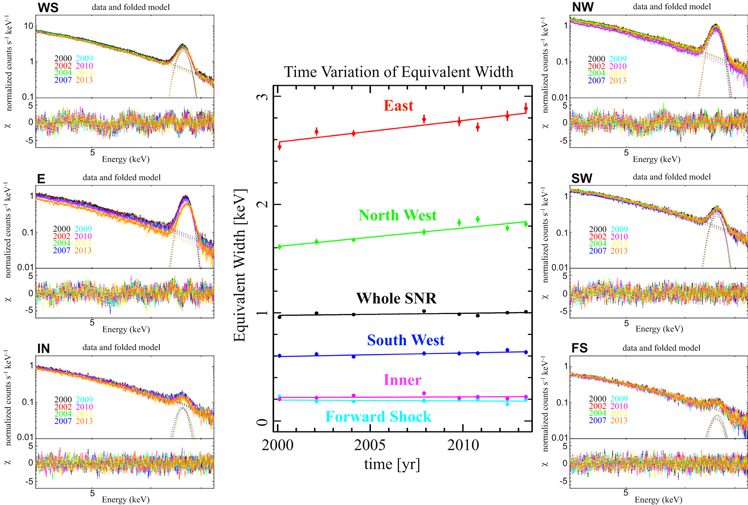
Figure 3. Time variation of the equivalent width of the Fe–K line (plot in the middle) and observed spectra in the 4.2–7.3 keV band (on both sides) at each region (whole SNR: WS, east: E, inner: I, north west: NW, south west: SW, forward shock: FS). In the central plot, the solid lines show best-fit linear models. Individual spectra were fitted with a model composed of a power law and a Gaussian. The error bars of all figures are 1σ.
Download figure:
Standard image High-resolution imageAs shown in Figure 3 and Table 3, we also found an increase of the equivalent width of the Fe–K line of Cassiopeia A for the first time. In the thermal dominant regions, we can see a ∼10% increase of the equivalent width for 13 years, and it is notable that a large evolution of the equivalent width like this is the first detection from all SNRs. In addition, we found the Fe–K line centroid varies among observations. Since there is a calibration uncertainty for Fe K-line centroids of ∼0.3% (or ∼20 eV at Fe–K)10 , however, it is difficult to discuss its evolution.
Table 3. Time Variation of Cassiopeia A in the 4.2–7.3 keV Banda
| 4.2–6.0 keV | Fe–K | Equivalent Width | ||
|---|---|---|---|---|
| (% yr−1) | (% yr−1) | (% yr−1) | ||
| Whole SNR | −0.65 ± 0.02 | −0.6 ± 0.1 | +0.2 ± 0.1 | |
| Thermal dominant region | ||||
| East | −1.03 ± 0.05 | −0.6 ± 0.1 | +0.8 ± 0.2 | |
| North West | −0.88 ± 0.04 | −0.2 ± 0.1 | +1.1 ± 0.2 | |
| Non-thermal dominant region | ||||
| South West | −0.60 ± 0.04 | −0.2 ± 0.3 | +0.6 ± 0.3 | |
| Inner | −0.46 ± 0.05 | −0.3 ± 0.9 | +0.3 ± 0.9 | |
| Forward Shock | +0.00 ± 0.07 | −0.0 ± 1.2 | −0.3 ± 1.0 | |
Note.
aErrors are at 90% confidence level.Download table as: ASCIITypeset image
3.3. Time Variation of 4.2–6.0 keV and Fe–K
From the fitting, we investigated the time variation of the 4.2–6.0 keV band and Fe–K line fluxes. Cassiopeia A flux evolution was well reproduced by linear decline (Patnaude et al. 2011). Therefore, we also fitted flux time variation with a linear model. These fitting results of each region are summarized in Figure 2 and Table 3. In the whole SNR, the 4.2–6 keV band and the Fe–K line fluxes show a significant decline in these ∼10 years with a similar change (∼−0.6% yr−1).
There is a discrepancy between the variation of the 4.2–6 keV band in this work, −0.65 ± 0.02% yr−1, and that in Patnaude et al. (2011), −1.5 ± 0.17% yr−1, in spite of nearly the same data set. Although we tried several analysis methods (see the
In the local regions, time variation of the 4.2–6.0 keV continuum and Fe–K line fluxes is different from the whole SNR. In Figure 4, we can see larger time variation of the 4.2–6 keV band in the regions which have higher equivalent width of the Fe–K line and a softer photon index. In addition, we also found the forward shock region has no significant change of 4.2–6 keV and Fe–K. From these results, we can interpret that Cassiopeia A is undergoing a flux change in the reverse shock region which has a larger Fe–K line contribution.
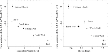
Figure 4. Left: plot of the change rate of the 4.2–6 keV continuum intensity versus the equivalent width of the Fe–K line. Right: plot of the change rate of the 4.2–6 keV continuum flux versus the photon index of the continuum power law. Equivalent width and photon index are the best fit values in the year 2000 (Table 2). Error bars are at the 90% confidence level.
Download figure:
Standard image High-resolution image3.4. Fitting the Spectra of the East Region with the Bremsstrahlung Model
As shown in Figure 4, we found that the east region has the largest decay rate and the largest equivalent width of the Fe–K line. Since the Fe–K line is a tracer of thermal plasma emission, we evaluated emission time variation from the east region via a thermal model. Table 4 shows the results of fitting with a thermal bremsstrahlung instead of the power-law model. We then drew time histories of the resultant temperature and normalization (= emission measure), and fitted them with a linear model. As a result, it is found that the time evolution of the temperature and the emission measure are −(0.4 ± 0.3)% yr−1 and −(0.5 ± 0.5)% yr−1 (90% confidence level), respectively.
Table 4. Best-fit Parameters of the Bremsstrahlung Model in the East Regiona
| Epoch | Bremss Model | χ2/d.o.f | |
|---|---|---|---|
| kT | Normalizationb | ||
| (Year) | (keV) | ||
| 2000.1 | 2.80
|
8.65
|
312.82/206 |
| 2002.1 | 2.69
|
8.95
|
307.28/206 |
| 2004.1 | 2.70
|
8.62
|
420.74/206 |
| 2007.9 | 2.68 ± 0.09 | 8.51
|
299.12/206 |
| 2009.8 | 2.66
|
8.41
|
278.59/206 |
| 2010.8 | 2.71
|
8.25
|
270.84/206 |
| 2012.4 | 2.67 ± 0.10 | 8.00
|
307.66/206 |
| 2013.4 | 2.54
|
8.63
|
292.35/206 |
Notes.
aErrors are at 1σ confidence level. b .
.
Download table as: ASCIITypeset image
4. Discussion
Patnaude et al. (2011) already reported intensity decay of the 4.2–6 keV continuum from the whole remnant of Cassiopeia A. They discussed the cause of the decay by assuming all emission originates from non-thermal emission. As shown in Figure 2 we found time variation in the whole remnant is also observed at the Fe–K line. Moreover, if we pick up the local regions, variabilities in the continuum and the Fe–K line are highly different from region to region. Therefore, the cause of the time variation in the 4.2–6 keV continuum and the Fe–K lines must be revisited. We positively used the fact that the Fe–K line is evidence of thermal emission. Then, we found the forward shock region which has faint Fe–K emission shows the smallest decay rate and the east region which has bright Fe–K emission shows the largest decay rate. The result naturally supports the idea that these regions have different variable components (thermal or non-thermal origin). Using these regions, we here discuss the origin of decay in the thermal dominant scenario (Section 4.1) and non-thermal dominant scenario (Section 4.2) individually.
4.1. A Decay Scenario of the Thermal Components
Young SNRs like Cassiopeia A are experiencing a drastic expansion due to the high speed of their ejecta. Plasma formed by shock heating should then be adiabatically expanded. Adiabatic expansion causes cooling of the plasma, too. Therefore, the change of X-ray flux from the thermal component must be first examined with an adiabatic cooling. Laming & Hwang (2003) suggested that Cassiopeia A is currently transitioning from the ejecta-dominated to the Sedov–Taylor phase, and hence it is natural to assume that Cassiopeia A is experiencing an adiabatic evolution without radiative cooling.
Here, we evaluate the time decay of regions where the thermal emission is dominant by assuming that their entire emission is of purely thermal origin. Bremsstrahlung X-ray flux from a thermal plasma is described as
where EM, h, kB, and  are the emission measure, Planck constant, Boltzmann constant, and Gaunt factor, respectively. The Gaunt factor is given by (see Rybicki & Lightman 1979)
where the constant ζ = 1.781. In the case of Cassiopeia A, a typical electron temperature is in the range of 1–3 keV (Hwang & Laming 2012). Therefore, we can use Equation (2) because the energy band we chose (4.2–6.0 keV) is above the spectrum cut-off.
First, we calculate the time evolution of the emission measure. We assume the number of particles nV = constant. Using the expansion parameter m (r ∝ tm), we can describe  ,
,  around a dynamical timescale or in the beginning of the Sedov–Taylor phase, and then

where we assume ne ∼ ni. In the case of Cassiopeia A, the emission measure change rate is
where we normalized m by 0.66 (Patnaude & Fesen 2009) and t by the remnant age of 340 year.
Next, we calculate the thermal decay rate by taking adiabatic cooling into account. For adiabatic gas, PVγ = const. By the same token, we can estimate temperature evolution along with the plasma volume as

where γ = 5/3 is the heat capacity ratio. Thus, we can estimate the rate of decline of temperature as
Here we can describe  and
and  . In order to calculate flux evolution including both of these effects,
  , and then
We measured a typical electron temperature of Cassiopeia A to be kBT ∼ 2.5 keV. This is about twice as low as the mean photon energy of the 4.2–6.0 keV band. Thus we can estimate the thermal component flux change rate as
The variation in the east region (=−1.03; see Table 3) is closest to this. Also, the predicted rates of the emission measure and temperature (see Equations (5) and (7)) are consistent with observational values in the east region; −(0.4 ± 0.3)% yr−1 for the emission measure and −(0.5 ± 0.5)% yr−1 for the temperature. Thus we conclude that flux variation in the east region of Cassiopeia A could be explained by thermal variation due to adiabatic expansion.
On the other hand, change rates in the other regions are much smaller than the value predicted by Equation (9). In particular, variations in the non-thermal dominant regions (<−0.6% yr−1) could not be explained by adiabatic expansion.
4.2. A Decay Scenario of the Non-thermal Components
Cosmic-ray electrons are considered to be accelerated in the shock front by diffusive shock acceleration (DSA; Bell 1978; Blandford & Eichler 1987). In the Sedov phase, the blast wave is decelerated by sweeping up ambient interstellar matter. This effect causes flux decay of synchrotron X-rays. In addition to this, evolution of the magnetic field and the electron injection rate also changes the flux of synchrotron X-rays. Here, we investigate whether the evolution of these parameters could explain the time variation of Cassiopeia A or not.
X-ray synchrotron emission is well approximated analytically. The electron energy spectrum is generally given by

where A, Eb, and  are a normalization factor, the break energy, and the maximum energy of electrons, respectively. In the case of Cassiopeia A, the radio index
  (Baars et al. 1977). The break energy expresses the spectrum shape which suffers synchrotron cooling. During acceleration, electrons with E > Eb are losing their energies via synchrotron cooling, which provides a steepened energy spectrum. From this electron distribution, we can calculate the approximate formula of the X-ray luminosity as shown in the Equation (5) of Nakamura et al. (2012),
where Bd, νb, and νroll are the downstream magnetic field, break frequency, and roll-off frequency, respectively. In this calculation, Nakamura et al. (2012) assumed photon energy is larger than break photon energy (ν > νb), and break frequency depends on the downstream magnetic field ( ). This assumption could be adapted for young SNRs (tage ≲ 103 year) due to their amplified magnetic field. Here, we attempted to estimate the time variation of the synchrotron X-ray in the case of Cassiopeia A by transforming this equation into our time evolution formulation framework.
First, we considered the time evolution of the normalization factor A in Equation (11). We assumed that the amount of accelerated particles is proportional to the product of the fluid ram pressure and the SNR volume, as assumed in Nakamura et al. (2012). Then, we can describe  , where vs is the shock velocity and we assume the shock is moving through the progenitor wind of the supernova: ρ ∝ r−2. Then the decay of this term is sensitive to the value of m. In the case of Cassiopeia A (m = 0.66), we find that this normalization is almost constant with time.
Second, we considered the time evolution of the term  in Equation (11). The magnetic energy density is amplified to a constant fraction of
  : case (a) or
  : case (a′) (e.g., Bell 2004; Vink 2006, 2008), and we can interpret the magnetic energy density evolution as a function of time as
Hereafter we denote  . If we neglect the time evolution of νroll for the time being, the discussion so far results in synchrotron intensity at the forward shock as Lν ∝ tX. Thus, we can estimate the time variation of the synchrotron radiation by the evolution of the magnetic field as
  . In the case of Cassiopeia A, m = 0.66: Patnaude & Fesen (2009), α = 0.77: Baars et al. (1977), and tage = 340 year predicts the variation of −0.08% yr−1 for case (a) and −0.09% yr−1 for case (a′), whose difference is quite small. From this result, we find that the contribution of the magnetic field evolution to the X-ray variation is small.
Finally, we consider the time evolution of the term  in Equation (11). Assuming that νroll is determined by a balance between the acceleration rate and synchrotron loss (Aharonian & Atoyan 1999; Yamazaki et al. 2006), we obtain
From the discussion of time evolution of all parameters (A, Bd, and νroll), the logarithmic derivative of Equation (11) results in (see also Katsuda et al. 2010)
In the case of Cassiopeia A, roll-off energy hνroll is suggested to be ∼2.3 keV in the outer shock filament (Grefenstette et al. 2015). This implies (ν/νroll) ≃ 2 for the band 4.2–6 keV. Thus, we can estimate the variation in the outer filament as  , and then a change rate is about −0.26% yr−1 for both cases (a) and (a′).
Consequently flux variability is sensitive to the value of the expansion parameter m. If we adopt m = 0.66, variation in the band 4.2–6 keV is estimated to be −0.26% yr−1. Figure 5 shows a comparison between the predicted rate and the observed time variation of the 4.2–6 keV continuum in the forward shock region. We found the model rate well fits observations from 2000 to 2010. The parameter m could be interpreted as a deceleration of the shock velocity. If we assume 5000 km s−1 as the shock velocity of Cassiopeia A, m = 0.66 means a deceleration of ∼5 km s−1 yr−1. In Figrue 5, however, the data points after 2010 do not follow the m = 0.66 line. For reference, we draw another line of m = 0.8 that is closer to the data after 2010. In this case the deceleration is ∼3 km s−1 yr−1. This means a strong braking in the shock velocity has not been occurring in the forward shock region (at most ∼5 km s−1 yr−1). We can see a flux jump between 2010 and 2012. Several non-thermal filaments in Cassiopeia A have a flickering of X-ray flux with a timescale of ∼year, and this jump might also be able to be explained by that feature.

Figure 5. Comparison between the time observed variation and the predicted change rate in the forward shock region in the band 4.2–6 keV. Black circles show our results of time variation in the forward shock (FS) region. Red solid and broken lines show the predicted change rate with m = 0.66 and m = 0.8, respectively.
Download figure:
Standard image High-resolution imageParticle acceleration and synchrotron cooling in the reverse shock are very complicated. The continuum emission seems to be decreasing gradually in the south west and inner regions. However, these regions have a number of flickering filaments and a large thermal X-ray contribution. In addition, the dynamical evolution of the reverse shock inward of the remnants have not been well understood. Zirakashvili et al. (2014) investigated particle acceleration in the forward and reverse shock of Cassiopeia A by using numerical calculations. They predicted the change rate of the synchrotron X-ray in the reverse shock to be ∼−0.9% yr−1 at least because ejecta density drops proportional to t−3 (=−0.9% yr−1). However, we cannot see such a large decrease in the south west and inner regions, and cannot explain the details of the acceleration in the reverse shock at present.
5. Conclusion
Our work shows the flux of the Fe–K line in Cassiopeia A is decreasing with continuum emissions in the 4.2–6 keV band for the first time. By using the hard X-ray distribution above 10 keV as a good indicator of non-thermal emission, we separated “thermal dominant” and “non-thermal dominant” regions from the whole SNR, and investigated their time variations. Then, we found clear correlations of the decay rates in the 4.2–6 keV band with photon indexes and with the equivalent width of the Fe–K line. The correlation shows that the flux in the regions which have a softer spectrum and richer emissions of Fe–K are decreasing more drastically.
We found the east region, which is considered to be the “thermal dominant” region and has the softest spectrum (Γ ∼ 3.2), shows the most rapid decline. The flux change rate of the Fe–K line and 4.2–6 keV continuum are −0.6 ± 0.1% yr−1 and −1.03 ± 0.05% yr−1, respectively. In the region, the time evolution of continuum flux, emission measure, and temperature are well explained by adiabatic cooling with the expansion of r ∝ t−m with m = 0.66.
On the other hand, “non-thermal dominant” regions show smaller decay rates. In particular, the forward shock region, which has the hardest spectrum (Γ ∼ 2.6), shows no large decay. It implies that the blast wave of Cassiopeia A does not seem to experience a strong deceleration (such as ≈30–70 km s−1 yr−1: Patnaude et al. 2011). From the decay rate, we conclude that deceleration is ∼5 km s−1 yr−1 at most.
It is interesting to note that the time evolution of the east region and the forward shock region, where thermal emission and non-thermal emission dominate the most among all selected regions, respectively, can be represented by the power-law expansion of r ∝ t−m with a common index of m = 0.66. Emission from the other regions is a certain mixture of thermal and non-thermal emission. Even though m = 0.66 is common, the resulting intensity decay rate is larger for thermal emission, and the intensity of the non-thermal continuum is nearly constant, if m does not change in the last couple of decades. A different mixing ratio probably results in an emission decay rate that is different from region to region. Accordingly, we conclude that the decay of X-ray intensity above ∼4 keV of the whole remnant is probably caused by the thermal emission component.
T.S. is grateful for travel support from HAYAKAWA FOUNDATION. This work was supported by the Japan Society for the Promotion of Science (JSPS) KAKENHI Grant Number 16J03448, 15K05107, 15K17657, 15K05088, 25105516, and 23540280. We thank Jacco Vink, Takayuki Hayashi, and Ryo Iizuka for helpful discussions and suggestions in preparing this paper. We thank the anonymous referee for his/her comments that helped us to improve the manuscript.
Appendix A: Difference of Arf and Source Region
We found an X-ray flux discrepancy between our results and those of Patnaude et al. (2011). Table 5 shows a comparison of our results with other results which are analyzed with different methods. In this table, we calculated X-ray flux and count-rate in the 4.2–6 keV band with several arfs and source regions for investigation of a cause of this discrepancy.
Table 5. Difference of Flux and Count-rate of the Whole SNR in the 4.2–6 keV Banda
| Fluxb | Count Ratec | |||||
|---|---|---|---|---|---|---|
| Epoch | Arf for Diffuse Source | Arf for Point Source | Patnaude et al. | |||
| (Year) | r = 3 |
r = 3 |
r = 2 |
r = 3 |
r = 2 |
|
| 2000 | 17.74
|
17.42
|
16.08
|
16.1 ± 0.1 | 6.76 ± 0.01 | 6.24 ± 0.01 |
| 2010 | 16.48 ± 0.03 | 16.48 ± 0.03 | 14.90
|
13.4 ± 0.1 | 5.91 ± 0.01 | 5.35 ± 0.01 |
| Ratio (2010/2000) | 0.929
|
0.946
|
0.923
|
0.832 ± 0.008 | 0.874 ± 0.002 | 0.857 ± 0.002 |
Notes.
aErrors are at 1σ confidence level. bFlux erg cm−2 s−1).
cCount rate (counts s−1).
erg cm−2 s−1).
cCount rate (counts s−1).
Download table as: ASCIITypeset image
In CIAO, we can calculate two kinds of arfs (weighted arf for extended sources or imaging arf for point-like source). We checked whether the types of arfs have an influence on the estimation of X-ray flux or not. The second and third columns in Table 5 show the 4.2–6 keV fluxes calculated by a weighted arf and an imaging arf, respectively. In this comparison, we cannot find a large difference, and cannot see a large decay from 2000 to 2010 like Patnaude et al. (see the fifth column). Therefore, a difference of arf type is not likely to be the cause of inconsistency. The fourth column in Table 5 shows the fluxes calculated by an imaging arf in a different source region (r = 25). The region within the 2
5 circle in Cassiopeia A does not include a part of the forward shock filaments (see Figure 6 left). In this case, the whole flux shows a lower value than 3
5 circle region, however flux decay from 2000 to 2010 does not change that much. In the count rate, we can see a larger decay than flux decay, as listed in the 6th and 7th columns of Table 5. This is because the effective area is decreasing with time. And, the decay of count rate within the 2
5 circle is very similar to that of Patnaude et al. (2011).
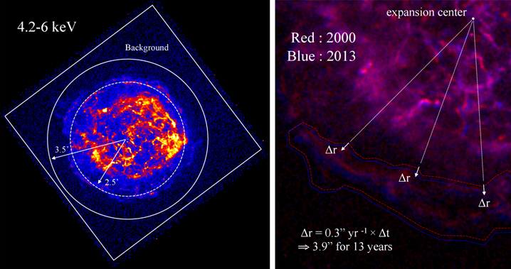
Figure 6. Left: source region difference. Radii of the broken circle and solid circle are r = 25 and r = 3
5, respectively. Right: region shift in the forward shock region. We shifted each apex of the polygon region to the expansion direction at 0
30% yr−1.
Download figure:
Standard image High-resolution imageAppendix B: Correction of Proper Motion Effect
The proper motion of Cassiopeia A’s forward shock has been well studied by X-rays (Patnaude & Fesen 2007), and its expansion rate is 030% yr−1 on average. If we discuss a flux variation in the forward shock, we define a region which is shifting with the forward shock region at this rate. We adopt a polygon shape as the shape of the forward shock region, and then we shift each apex to the expansion direction at 0
30% yr−1 (see Figure 6 right). If we do not adapt this region shift, we find the flux in 2013 is ∼5% higher than that in 2000 because a component which was exterior to the region 13 years ago leaked inside the region. In the reverse shock region, there are fewer leak contributions than in the forward shock since the proper motion of the reverse shock is small. When we adapt the region shift to the east region, it is found that the decay rate does not change. Therefore, we have not adopted the region shift in the reverse shock regions.
Footnotes
- 10
Available at http://cxc.harvard.edu/cal/docs/cal_present_status.html.