Abstract
The present work explores the origin of the formation of star clusters in our Galaxy and in the Small Magellanic Cloud (SMC) through simulated H-R diagrams and compare those with observed star clusters. The simulation study produces synthetic H-R diagrams through the Markov Chain Monte Carlo (MCMC) technique using the star formation history (SFH), luminosity function (LF), abundance of heavy metal (Z), and a big library of isochrones as basic inputs and compares them with observed H-R diagrams of various star clusters. The distance-based comparison between those two diagrams is carried out through two-dimensional matching of points in the color−magnitude diagram (CMD) after the optimal choice of bin size and appropriate distance function. It is found that in a poor medium of heavy elements (Z = 0.0004), the Gaia LF along with a mixture of multiple Gaussian distributions of the SFH may be the origin of formation of globular clusters (GCs). On the contrary, an enriched medium (Z = 0.019) is generally favored with the Gaia LF along with a double power law or Beta-type (i.e., unimodal) SFH, for the formation of globular clusters. For SMC clusters, the choice of an exponential LF and exponential SFH is the proper combination for a poor medium, whereas the Gaia LF with a Beta-type SFH is preferred for the formation of star clusters in an enriched medium.
1. Introduction
The Hertzsprung−Russell (H-R) diagram is a bivariate plot of absolute magnitude versus temperature or color for a large number of stars in resolved stellar populations or galaxies. This diagram provides a snapshot of the evolutionary status of the stars that are bright enough to be detected. Various parameters like star formation histories (SFHs), luminosity functions (LFs), chemical abundance, or metallicity (Z) etc., interact in a significant way, which in turn determines the shape of the H-R diagram in composite stellar populations. The stellar populations are much more complex systems containing numerous different star formation epochs superimposed upon a single H-R diagram. Thus, H-R diagrams or color–magnitude diagrams (CMD) require more sophisticated techniques for accurate interpretation.
The most common technique to interpret a CMD is to produce a series of isochrones (stars that are at the same time and metallicity in their evolutionary status). These will match as many characteristics of the diagram as possible and thus are either older or younger in age than the majority of the stars (Miller et al. 2001; Jørgensen & Lindegren 2005; Monteiro et al. 2010). Also, this verification method is appropriate for CMDs of star clusters that are created at a single point of time (Sandage 1953, 1958; Stetson 1993; Kalirai & Tosi 2004). But recent studies show that resolved stellar populations have not originated at a single epoch but at multiple epochs (Mackey et al. 2008; Katz & Ricotti 2013; Bastian & Lardo 2018). Thus, a possible way to properly interpret a complex CMD is through a statistical (Monte Carlo) simulation where a composite stellar population can be generated from evolutionary tracks using LFs, SFHs, and metallicities and matched with the observed ones to properly interpret their origin. The above discussion is the motivation behind the present work. A similar idea was first applied to galaxies (Ferraro et al. 1989), and elaborate models were developed (Tosi et al. 1991; Bertelli et al. 1992; Greggio et al. 1993; Hernandez et al. 1999). The unveiling of an unknown SFH incorporating measurement errors was studied by Tolstoy & Saha (1996). Parametric models for galaxy SFHs were developed by Carnall et al. (2019), and the role of various SFHs was studied in the photometry of these objects. Attempts have been made to make comparisons between synthetic CMDs and observed CMDs by Arp (1967), Robertson (1974), Harris & Deupree (1976), Flannery & Johnson (1982), Becker & Mathews (1983), Salaris et al. (2007), Fiorentino et al. (2011), and Martins & Palacios (2017), among others.
Statistically reliable methods were also previously used by various authors for comparing synthetic (simulated) and observed data sets in X-ray astronomy (Lampton et al. 1976; Sarazin 1980; Bradt et al. 1992; Ramsey et al. 1994; Gruber et al. 1999) and in quasar distribution (Peacock 1983; Fasano & Franceschini 1987). These techniques have been used in situations where a functional form of the distributions is available. On the contrary, a CMD model is a complex two-dimensional nonlinear distribution of data points, and it is important to take into consideration the fact that the two sets of data points match with respect to spatial distribution as well as the relative number of points at different positions in the diagram.
In the present work, we have considered SFHs, LFs, and metallicities as the basic inputs for producing a synthetic H-R diagram and then matched the synthetic diagrams to the observed ones for resolved stellar populations to explore their origins. The present work has the following improvements over previous works:
- 1.We have used different SFHs instead of a single SFH.
- 2.
- 3.We have matched the CMD diagrams of observed and synthetic ones by computing “minimum distances” between the bivariate histograms. This takes into consideration both the spatial and probability distributions.
- 4.We have optimized the “bin” size and “distance function” through comparison with other bin sizes and distance functions existing in the literature.
In Section 2, we develop the mathematical model. In Section 3, the various forms of the SFHs are discussed. Section 4 describes both the observed and theoretical LFs used in the work. Section 5 gives a short description of the matching model. Results and discussions are demonstrated in Section 6. Section 7 outlines our conclusions.
2. The Model
To produce a synthetic CMD, we first assume an SFH, i.e., SFR(t) (star formation rate as a function of time) and an LF. The CMD requires a method of obtaining the color and luminosity (or absolute magnitude) of a star of given mass and age. To find the color and luminosity at a given age and metallicity, various theoretical isochrones are used. If the isochrones are largely spaced over time, then interpolation between isochrones will be an erroneous procedure that can introduce spurious structure into the ultimate result. To avoid such error, we use the latest Padova (Fagotto et al. 1994; Girardi et al. 2000) full stellar tracks, calculated at fine variable time intervals, and a careful interpolation method is used at constant evolutionary phases to construct an isochrone library. We have constructed almost 1000 points in each isochrone, so that the luminosity resolution is very small. Also, we have taken two metallicity limits, Z = 0.0004 and Z = 0.019, i.e., the minimum and maximum values, to explore the effect of metallicity, if any, on the origin and hidden properties of stellar populations. We fit linear splines to the isochrones at l evenly spaced luminosity intervals given a tabulated function yi = y(xi ), i = 1, 2, 3,…,lj , j, with j being the jth isochrone.
For i = 1, 2, 3,…,lj , the interpolating function joins (lj − 1) linear functions of the form

where ai
and bi
are constants satisfying (i) fi
(xi
) = yi
and (ii) fi
(xi+1) = yi+1, i.e.,  and
and  , i = 1, 2,…,(lj
− 1).
, i = 1, 2,…,(lj
− 1).
Then, we start again with newly interpolated points along with the old ones and repeat the process to include more interpolating points. We repeat the same procedure for all other isochrones. This decreases the interpolation error (Cassisi et al. 2012). Figure 1 shows one such original isochrone along with the interpolated isochrone formed using linear interpolation, iteratively used.
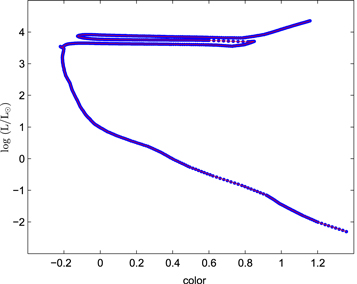
Figure 1. Interpolated points (1200; in red) on a particular original isochrone (in blue) of 50 points at time = 0.0634 Gyr and metallicity Z = 0.0004. The luminosity (l; i.e.,  ) is along the vertical axis and the color (c) is along the horizontal axis.
Download figure:
Standard image High-resolution imageTo produce a synthetic CMD, the following steps are performed:
- 1.One possible choice of probability density function (pdf) of SFR(t) is considered.
- 2.One particular choice of LF is considered.
- 3.One time point t is randomly generated from the SFR(t) distribution.
- 4.One luminosity point (l) is randomly generated from LF distribution.
- 5.The color (c) corresponding to the time (t) and luminosity (l) is extracted from the interpolated isochrone library.
- 6.Steps (3)−(5) are repeated a large number of times (5000 in our case).
- 7.The various luminosities (li ) and colors (ci ), i = 1, 2,…, 5000, are plotted, which is the synthetic CMD in our case.
- 8.The synthetic CMD is compared with various observed CMD diagrams of open and globular clusters, and the matched pair for which the spatial distance is minimum is chosen.
3. Various Star Formation Histories
Following Carnall et al. (2019), three SFH models are considered. They are:
- 1.
- 2.
- 3.
In addition, we have also considered a Gaussian mixture model (two and three modes) following the episodic nature of star formation (Hernandez et al. 1999; Stinson et al. 2007; Tremblay et al. 2010; Huang et al. 2013; Debsarma et al. 2016; Cignoni et al. 2018; Das et al. 2020) and a Beta distribution following unimodal star formation history in many giant galaxies.
3.1. Exponentially Declining SFR(t)
Exponentially declining SFHs are a widely used model of SFH. In this model, the star formation jumps from zero to its maximum value at some time T0, after which star formation declines exponentially with some timescale τ, i.e.,

Here, T0 ∼ (0, 15) Gyr and τ ∼ (0.3, 10) Gyr (Carnall et al. 2019).
Hence, for a pdf, SFR  , where,
  and T0 = 0. This is the standard form of a negative exponential pdf.
The exponential model is often used as a fiducial model, and they are less appropriate at higher redshifts (Reddy et al. 2012). They have some bias when the stellar mass, star formation rate (SFR), and mass-weighted age are reproduced by fitting mock observations of simulated galaxies (Simha et al. 2014; Pacifici et al. 2016; Carnall et al. 2019).
3.2. Delayed Exponentially Declining SFR(t)
Sometimes, delayed exponentially declining SFHs are more realistic than the ordinary exponential type. As the stars are formed, they take some time to evolve from the main sequence to giant form, and ultimately end their lives in a supernova explosion in the case of very massive stars. The ejection of material from the supernova enriches the medium for a second generation of star formation, and there is a delay in recycling the material (Pagel & Tautvaisiene 1995). This results in a merely flexible and physical model of star formation and shows a rising SFH if τ is large. Thus,
where T0 ∼ (0, 15) Gyr, and τ ∼ (0.3, 10) Gyr.
3.3. Double Power-law SFR(t)
Here the rising and falling slopes of the SFH are different over time and are denoted by β and α, respectively. The function shows a good fit to the redshift evolution of the cosmic SFR density (Behroozi et al. 2013; Gladders et al. 2013) as well as producing a good fit to SFHs from simulations (Pacifici et al. 2016; Diemer et al. 2017; Carnall et al. 2019). Thus,

where α ∼ (0.1, 1000) is the falling slope, β ∼ (0.1, 1000) is the rising slope, and τ ∼ (0.1, 15) Gyr is related to the peak time.
3.4. Gaussian Mixture Modeling SFR(t)
The Gaussian mixture also reflects the episodic nature of star formation in many dwarf galaxies as observed by various authors (Lee et al. 2012; Weisz et al. 2014). The common form of the Gaussian mixture model is

where g1(t) and g2(t) are two Gaussian pdfs with parameters (μ1, σ1) and (μ2, σ2), respectively and

where g1(t), g2(t), g3(t) are three Gaussian pdfs with parameters (μ1, σ1), (μ2, σ2), (μ3, σ3) in case of a mixture of three Gaussian distributions, and q1, q2 are the weights lying between 0 and 1. All of the samples are generated using the Markov Chain Monte Carlo method (Robert & Casella 2004), where we have used a Uniform distribution U[0, 1] as the prior distribution.
3.5. Beta Distribution of SFR(t)
The standard Beta distribution is of the form
where p, q > 0 are, respectively, the rising and falling slopes of the SFH over time and B(p, q) =  , where Γ is the Gamma function. A unimodal SFR (SFR(t)) has been seen in many giant galaxies (Debsarma et al. 2016; Feldmann 2017; Das et al. 2020) under various parametric conditions. Here we consider the values of (p, q) to be (2, 2) and (5, 1), respectively.
4. Luminosity Functions
4.1. Observed Luminosity Function in the Gaia Catalog
In the Gaia catalog (Brown et al. 2018),
4
from the first table of 169,29,19,135 observations, a few parameters like Gmag (first one in the fourth block; here written as mG
), Plx (10th one in the first block), and AG (ninth one in the sixth block) are considered, where mG
, Plx and AG are the apparent magnitudes, parallaxes, and extinction parameters in the G band. The sample is restricted to Plx <20″ to avoid errors to a large extent. This reduces the sample size from 169,29,19,135 to 69,92,398. Thus, we obtain 69,92,398 observations from the set (for those whose AG values exist and have positive parallaxes). The observed apparent magnitude mG
(in the G band) from the Gaia data set are transformed to extinction-corrected absolute magnitude  using the Pogson relations,

Then, these  are converted to luminosity using

Luminosities thus obtained are fitted to a mixture of the normal distribution of the form

The maximum-likelihood estimates of the above distribution came out to be  ,
,  ,
,  ,
,  , and
, and  , respectively, with a p value of 0.2216. Figure 2 shows the luminosity values with the fitted curves.
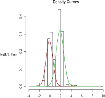
Figure 2. Luminosity function fitted to the reduced Gaia Mission data set.
Download figure:
Standard image High-resolution image4.2. Truncated Power Law
There are various observations of the LFs of young massive clusters, for example, the Arches cluster (Figer et al. 1999), NGC 3603 (Sung & Bessell 2004; Stolte et al. 2006; Harayama et al. 2008; Portegies Zwart et al. 2010), and Westerlund 1 (Brandner et al. 2008), which are of truncated power-law form. So we have also considered a truncated power law for a typical luminosity function. This has the form
where β, ν are the lower and upper values of the luminosities in the isochrones, used in the model (i.e., log10(L/L⊙) ∼ −2 to +4, α ∼ 1.05).
Whitmore et al. (2014) observed 20 nearby (4−30 Mpc) star clusters in star-forming galaxies based on ACS source lists generated by the Hubble Legacy Archive. A typical cluster LF is fitted by a power-law pdf of the form

where λ varies from 1.95 ± 0.02 to −3.09 ± 0.46. All of the galaxies in the catalog are of Sa type and their absolute magnitudes (MB ) in the B band vary from −17.46 to −20.96. We have considered a few values of λ in the simulation study to investigate the effect of luminosity functions in external galaxies.
5. Matching Criteria between Simulated and Observed Stellar Population Distributions
5.1. Choice of Dissimilarity Measure
In this section, we address the problem of comparing two histograms corresponding to observed and simulated distributions. We can use a good dissimilarity measure as this can be used as an inverse matching criterion. The higher the value of the measure, the lesser the degree of similarity between the two distributions. So, for good measure, the value should be significantly lower while matching two different types of distributions and close to zero for two very similar distributions.
It is well known that the Chi-square distance function is a very good dissimilarity measure (Pele & Werman 2010; Yang et al. 2015; Greenacre 2017) for comparing two histograms.
If pj and qj are the probabilities (frequency densities) corresponding to the jth class (j = 1, 2,…,k) of the two histograms under consideration, then the Chi-square distance function is given by
i.e., pj
and qj
correspond to the bin values of the jth class with respect to the two histograms under consideration.  satisfies all the necessary properties of a dissimilarity measure.
5.2. Tuning of the Optimum Bin Size
While drawing the histogram, it is necessary to choose the bin size optimally by taking into consideration the dissimilarity measure and the ranges of the variables under consideration. In order to study the discriminating power of the dissimilarity measure and to choose the optimum bin size, we have defined the following metric.
We have several simulated (model) data sets. We have primarily chosen one simulated data as the anchor data set and some observed similar and dissimilar data sets through physical consideration. Then, the metric under consideration is metric = (mean value of the dissimilarity measure between the anchor data set and the observed dissimilar data set) − (mean value of the dissimilarity measure between the anchor data set and the observed similar data set).
Here, the mean is taken over observed dissimilar data sets and similar data sets respectively in first and second term of the metric.
The discrimination power for a particular dissimilarity measure is higher when the value of the metric (i.e., difference) for the measure increases with respect to similar and dissimilar data sets. This means that the metric will have a higher value because the mean distance between the anchor and dissimilar observed data set will be larger and the distance between the anchor and observed similar data set will be smaller.
One thing to note is that the bin size also depends on the ranges of the histogram. At the time we computed the dissimilarity measure between one model data set and one observed data set while calculating the minimum and maximum ranges of the variables, we include the variables of the model and observed data sets along with the anchor, similar, and dissimilar data sets.
With the calculated range values, we did optimum bin size tuning on the anchor, similar, and dissimilar data sets (but with only the Chi-Square distance) as described above and calculated the optimum bin size for which the metric value becomes largest. Finally, with the optimum bin size value, we compared the normalized histograms for a pair of model and observed data sets and then calculate the dissimilarity with the Chi-Square distance. The whole algorithm is tabulated in Algorithm 1. In Table 1, it can be seen that while calculating the validation metric for the mentioned observed data and anchor data sets, we find that for bin size 50, the metric is largest with a value of 0.5074. So, 50 is the optimum bin size while calculating the dissimilarity between the mentioned two data sets. The above exercise is followed for the comparison of every pair of model data set and observed data set.
Table 1. As the Optimum Bin Size Depends on the Range of the Data, the Range of the Histogram is Calculated by Taking the Union of the Ranges of the Validation Sets, which are the Anchor Data Set: Gaussian SFR(t) with Two Modes (Means ∼2, 11 and sds ∼0.3, 0.2 and Equal Weights); Observed Similar Data Sets: M53 and NGC 1904 GCs; Observed Dissimilar Data Sets: H and χ Persei, NGC 2264, NGC 7160 Open Clusters; and Data Sets to be Compared: H and χ Persei (an Open Cluster) and Simulated Data Set for Gaussian SFR(t) with Three Modes (Means ∼9, 11, 13 and sds ∼0.05, 0.05, 0.05) and Gaia LF
| Bin Size | Metric on Chi-Square Distance |
|---|---|
| 10 | 0.5067 |
| 20 | 0.4881 |
| 30 | 0.4864 |
| 40 | 0.5000 |
| 50 | 0.5074 |
| 60 | 0.5021 |
| 70 | 0.4962 |
| 80 | 0.4870 |
| 90 | 0.4985 |
| 100 | 0.4852 |
Note. The metric is calculated with respect to the anchor data set and the observed similar and dissimilar data sets once the ranges are adjusted. Finally, the Chi-square distances are calculated between the pair to be compared once the bin size is tuned, which is 50 for the above pair.
Download table as: ASCIITypeset image
Algorithm 1. Optimum Bin Size Selection Algorithm
| 1: | Calculate the minimum and maximum of the ranges of the color variable from the validation data sets (anchor, similar, and dissimilar data sets), model data set, and observed data set. |
| 2: | Calculate the minimum and maximum of the ranges of the log (L/L⊙) variable from the validation data sets (anchor, similar, and dissimilar data sets), model data set, and observed data set. |
| 3: |
for
 do
do
|
| 4: | Calculate the metric from the above metric calculation equation using the Chi−Squared distance. |
| 5: | Find the bin size for which the metric value is maximum. |
| 6: | Build normalized histograms for both model and observed data. |
| 7: | Calculate Chi−Squared dissimilarity measure for the above two histograms. |
Download table as: ASCIITypeset image
5.3. Actual Data Analysis
Here, our objective is to compare several observed CMDs with possible simulated CMDs generated under different model assumptions. For each CMD, we have data for two variables, viz. “color” and “luminosity” (viz. log (L/L⊙)), we have to draw one normalized bivariate histogram corresponding to each CMD. As shown in Table 1, the optimum bin size may be taken to be 50 × 50 for each such bivariate histogram as the ranges of each of the two variables are almost similar for all data sets under consideration (both in Section 5.1 and Section 5.2).
Then, we have computed the Chi-square dissimilarity measure values for different pairs of simulated (model) and observed CMDs in order to find out the possible matches. The simulated CMDs, i.e., synthetic H-R diagrams, have been generated using Monte Carlo simulation under various choices of the concerned parameters.
Figures 3–4 represent simulated CMDs generated using Monte Carlo simulation for different choices of parameters like SFH, LF, and metallicity. Figure 5 illustrates the comparison between the simulated (in red) and observed (in cyan) CMD (including normalized count) for the SMC Brück 2 star cluster with optimum bin size to calculate the Chi-squared dissimilarity value. Figures 6–7 have similar representations but for observed H and χ Persei (an open cluster) and 47 Tuc (Milky Way globular cluster, MW GC), respectively.
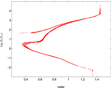
Figure 3. Synthetic H-R diagram for a bimodal Gaussian (two modes) type of SFH (i.e., SFR(t)) (μ1 = 11, σ1 = 0.2, μ2 = 13, σ2 = 0.5, q = 0.5), LF = Gaia LF, and Z = 0.0004.
Download figure:
Standard image High-resolution image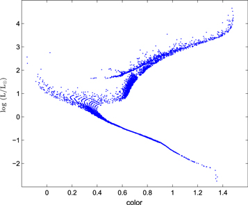
Figure 4. Synthetic H-R Diagram for a Beta distribution of the SFH (i.e., SFR(t)) with parameters p = 2, q = 2, LF = Gaia LF, and Z = 0.0004.
Download figure:
Standard image High-resolution image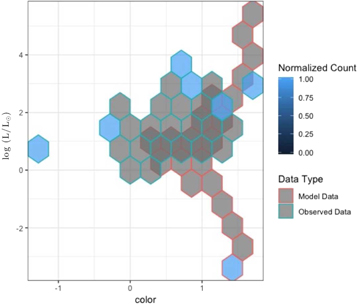
Figure 5. (a) Comparison of normalized histograms and (b) scatter plots between the observed data: SMC Brück 2 (a SMC star cluster) and model data: with Gaussian (three modes) SFR(t) (means ∼2, 5, 7 and sds ∼0.05, 0.05, 0.05) and Gaia LF and Z = 0.0004. Here, the bin size is 10 and the Chi-squared dissimilarity value is 0.265.
Download figure:
Standard image High-resolution image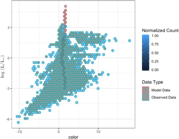
Figure 6. (a) Comparison of normalized histograms and (b) scatter plots between observed data: H and χ Persei (an open MW cluster) and model data with Gaussian (two modes) SFR(t) (means ∼2, 8 and sds ∼0.2, 0.5, respectively), Gaia LF, and Z = 0.0004. Here, the bin size is 50, and the Chi-squared dissimilarity value is 0.577.
Download figure:
Standard image High-resolution image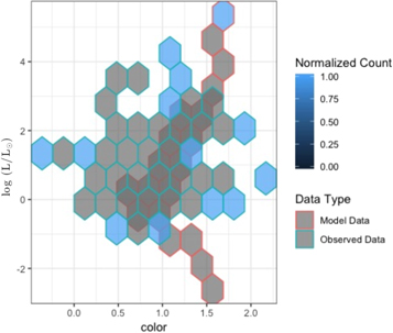
Figure 7. (a) Comparison of normalized histograms and (b) scatter plots between observed Data: 47 Tuc (MW GC) and model data with SFR(t) of Gaussian (3 modes) type (means ∼2, 5, 7 and sds ∼0.05, 0.05, 0.05) and Gaia LF and Z = 0.019. Here, the bin size is 10, and the Chi-squared dissimilarity value is 0.086.
Download figure:
Standard image High-resolution image6. Results and Discussions
6.1. Properties of the Synthetic H-R Diagrams
Synthetic H-R diagrams have been generated using Monte Carlo simulation under various SFHs, luminosity profiles, and metallicities, and the diagrams have been compared to various star clusters, both Galactic or globular clusters, to explore the origin of these star clusters. The matching is carried out through an algorithm of finding the minimum distance between any pair of choice, viz. the synthetic H-R diagram and observed star cluster. The details of the procedure have been outlined in Section 5. Finally, the pair with minimum distance (in bold digits) has been chosen as the pair for comparison. The values of the dissimilarity measures having values <1.0 have been listed in various tables (Tables 2–16). The properties of GCs (metallicities and Galactocentric distances, etc.) are from the Harris (1996) updated catalog (listed in Table 2); similarly, the properties (metallicities and distances) of SMC star clusters (listed in Table 3) and MW open clusters (listed in Table 4) are taken from Dias et al. (2016) and Dias et al. (2002), respectively. The following observations have been reflected in the tables.
Table 2. Comparison of Synthetic H-R Diagrams Using the Gaia LF, Z = 0.0004 with Observed MW GCs for Various SFR(t)
| Names | Metallicitya | a Galacto- | DPL | DPL | β | β | DE | E | E | G3 | G3 | G2 | G2 |
|---|---|---|---|---|---|---|---|---|---|---|---|---|---|
| of | [Fe/H] | centric | (α, β) | (α, β) | (p, q) | (p, q) | (T0, τ) | (λ) | (λ) | (μ1, σ1) | (μ1, σ1) | (μ1, σ1) | (μ1, σ1) |
| Observed | Distances | (τ) | (τ) | (μ2, σ2) | (μ2, σ2) | (μ2, σ2) | (μ2, σ2) | ||||||
| Star | (kpc) | (50, 0.2) | (50, 10) | (2, 2) | (5, 1) | (15, 9) | (5) | (10) | (μ3, σ3) | (μ3, σ3) | (q) | (q) | |
| Clusters | (15) | (15) | (q1, q2) | (q1, q2) | |||||||||
| (9, 0.05) | (2, 0.05) | (2, 0.2) | (11, 0.2) | ||||||||||
| (11, 0.05) | (5, 0.05) | (8, 0.5) | (13, 0.5) | ||||||||||
| (13, 0.05) | (7, 0.05) | (0.5) | (0.5) | ||||||||||
| (0.5, 0.3) | (0.5, 0.3) | ||||||||||||
| 47 Tucanae | −0.76 | 7.4 | 0.4600 | 0.4525 | 0.4573 | 0.4562 | 0.4748 | 0.5857 | 0.5881 | 0.4557 | 0.1901 | 0.1238 | 0.450 |
| (Alcaino et al. 1987) | |||||||||||||
| M14 | −1.39 | 4.1 | 0.7743 | 0.7738 | 0.7556 | 0.7730 | 0.7599 | 0.8791 | 0.9102 | 0.7729 | 0.2883 | 0.3204 | 0.7730 |
| (Contreras et al. 2013) | |||||||||||||
| M5 | −1.27 | 6.2 | 0.3143 | 0.3136 | 0.3130 | 0.3144 | 0.3319 | 0.4411 | 0.4428 | 0.3189 | 0.1182 | 0.1257 | 0.3089 |
| (Sandquist et al. 1996) | |||||||||||||
| M92 | −2.28 | 9.6 | 0.3402 | 0.3503 | 0.3411 | 0.3422 | 0.3431 | 0.4415 | 0.4421 | 0.3468 | 0.2626 | 0.2354 | 0.3451 |
| (Stetson & Harris 1988) | |||||||||||||
| M53 | −1.99 | 18.3 | 0.7976 | 0.8202 | 0.7918 | 0.8285 | 0.8079 | 0.7787 | 0.7939 | 0.8223 | 0.5366 | 0.5396 | 0.8270 |
| (Heasley & Christian 1991) | |||||||||||||
| NGC 1261 | −1.35 | 18.2 | 0.6196 | 0.5895 | 0.5755 | 0.5762 | 0.5834 | 0.6749 | 0.6982 | 0.5830 | 0.3681 | 0.4407 | 0.5795 |
| (Alcaino et al. 1992) | |||||||||||||
| NGC 1904 | −1.57 | 18.8 | 0.8791 | 0.9972 | 0.9972 | 0.9972 | 0.9972 | 0.9972 | 0.8788 | 0.9972 | 0.8789 | 0.8795 | 0.9972 |
| (Kravtsov et al. 1997) | |||||||||||||
| NGC 2808 | −1.15 | 11.1 | 0.6506 | 0.6605 | 0.6413 | 0.6502 | 0.6506 | 0.7958 | 0.7924 | 0.6585 | 0.2276 | 0.2298 | 0.6492 |
| (Sosin et al. 1997) | |||||||||||||
| NGC 288 | −1.24 | 12.0 | 0.6175 | 0.6291 | 0.6147 | 0.6172 | 0.6311 | 0.7142 | 0.7160 | 0.6310 | 0.3609 | 0.2985 | 0.6162 |
| (Alcaino et al. 1997a) | |||||||||||||
| NGC 3201 | −1.58 | 8.9 | 0.7456 | 0.7282 | 0.7217 | 0.7281 | 0.7426 | 0.8494 | 0.8442 | 0.7361 | 0.2428 | 0.2762 | 0.7253 |
| (Layden & Sarajedini 2003) | |||||||||||||
| NGC 362 | −1.16 | 9.4 | 0.6795 | 0.6654 | 0.6624 | 0.6527 | 0.6699 | 0.8565 | 0.8589 | 0.6679 | 0.3940 | 0.3304 | 0.6530 |
| (Green & Norris 1990) | |||||||||||||
| NGC 4147 | −1.83 | 21.3 | 0.5603 | 0.5268 | 0.5264 | 0.5152 | 0.5395 | 0.6533 | 0.6751 | 0.5286 | 0.4323 | 0.3569 | 0.5159 |
| (Wang et al. 2000) | |||||||||||||
| NGC 4372 | −2.09 | 7.1 | 0.8031 | 0.7998 | 0.7995 | 0.7996 | 0.8074 | 0.9358 | 0.9324 | 0.8047 | 0.2667 | 0.2800 | 0.7984 |
| (Alcaino et al. 1991) | |||||||||||||
| NGC 4590 | −2.06 | 10.1 | 0.4956 | 0.4500 | 0.4586 | 0.4427 | 0.4693 | 0.7291 | 0.7512 | 0.4513 | 0.1920 | 0.2850 | 0.4422 |
| (Walker 1994) | |||||||||||||
| NGC 4833 | −1.80 | 7.0 | 0.6269 | 0.6752 | 0.6533 | 0.6653 | 0.6596 | 0.8189 | 0.8233 | 0.6741 | 0.2131 | 0.2181 | 0.6619 |
| (Melbourne et al. 2000) | |||||||||||||
| NGC 5466 | −2.22 | 16.2 | 0.4269 | 0.3994 | 0.4036 | 0.3908 | 0.4135 | 0.6733 | 0.6791 | 0.4000 | 0.1939 | 0.2789 | 0.3929 |
| (Buonanno et al. 1984) | |||||||||||||
| NGC 5694 | −1.86 | 29.1 | 0.5461 | 0.5471 | 0.5382 | 0.5357 | 0.5317 | 0.6657 | 0.6714 | 0.5329 | 0.3624 | 0.4077 | 0.5416 |
| (Ortolani & Gratton 1990) | |||||||||||||
| NGC 5927 | −0.37 | 4.5 | 0.9033 | 0.9080 | 0.9021 | 0.9078 | 0.9033 | 0.9365 | 0.9418 | 0.9079 | 0.3487 | 0.4026 | 0.9077 |
| (Samus et al. 1996) | |||||||||||||
| NGC 6121 | −1.20 | 5.9 | 0.8348 | 0.8463 | 0.8442 | 0.8465 | 0.8459 | 0.9131 | 0.9147 | 0.8480 | 0.3208 | 0.4010 | 0.8447 |
| (Kanatas et al. 1995) | |||||||||||||
| NGC 6171 | −1.04 | 3.3 | 0.9268 | 0.9261 | 0.9267 | 0.9242 | 0.9267 | 0.9686 | 0.9708 | 0.9276 | 0.9401 | 0.9314 | 0.9256 |
| (Ferraro et al. 1991) | |||||||||||||
| NGC 6205 | −1.54 | 8.7 | 0.3276 | 0.3556 | 0.3261 | 0.3458 | 0.3391 | 0.3822 | 0.3739 | 0.3528 | 0.1494 | 0.1801 | 0.3462 |
| (Cohen et al. 1997) | |||||||||||||
| NGC 6218 | −1.48 | 4.5 | 0.5194 | 0.5693 | 0.5337 | 0.5761 | 0.5558 | 0.6059 | 0.6085 | 0.5722 | 0.3230 | 0.3006 | 0.5721 |
| (Sato et al. 1989) | |||||||||||||
| NGC 6254 | −1.52 | 4.6 | 0.6713 | 0.7139 | 0.6722 | 0.7142 | 0.6927 | 0.7183 | 0.7335 | 0.7160 | 0.2532 | 0.3165 | 0.7124 |
| (Hurley et al. 1989) | |||||||||||||
| NGC 6352 | −0.70 | 3.3 | 0.8565 | 0.8555 | 0.8536 | 0.8561 | 0.8561 | 0.8974 | 0.9032 | 0.8557 | 0.2981 | 0.2662 | 0.8552 |
| (Fullton et al. 1995) | |||||||||||||
| NGC 6356 | −0.50 | 7.6 | 0.9176 | 0.9208 | 0.9219 | 0.9197 | 0.9229 | 0.9575 | 0.9529 | 0.9208 | 0.3718 | 0.2662 | 0.9193 |
| (Bica et al. 1994) | |||||||||||||
| NGC 6362 | −0.95 | 5.1 | 0.7423 | 0.7589 | 0.7496 | 0.7458 | 0.7624 | 0.8285 | 0.7922 | 0.7593 | 0.4152 | 0.4846 | 0.7452 |
| (Brocato et al. 1999) | |||||||||||||
| NGC 6397 | −1.95 | 6.0 | 0.5459 | 0.5494 | 0.5312 | 0.5520 | 0.5548 | 0.6191 | 0.6376 | 0.5512 | 0.2805 | 0.2796 | 0.5487 |
| (Alcaino et al. 1997b) | |||||||||||||
| NGC 6553 | −0.21 | 2.2 | 0.9954 | 0.9999 | 0.9940 | 0.9999 | 0.9988 | 0.9879 | 0.9879 | 0.9999 | 0.4247 | 0.4996 | 0.9999 |
| (Sagar et al. 1999) | |||||||||||||
| NGC 6624 | −0.44 | 1.2 | 0.4130 | 0.4090 | 0.4105 | 0.4228 | 0.4305 | 0.5118 | 0.5326 | 0.4147 | 0.3449 | 0.3001 | 0.4162 |
| (Heasley et al. 2000) | |||||||||||||
| NGC 6637 | −0.70 | 1.9 | 0.8578 | 0.8740 | 0.8622 | 0.8737 | 0.8686 | 0.9331 | 0.9374 | 0.8755 | 0.2825 | 0.2554 | 0.8727 |
| (Heasley et al. 2000) | |||||||||||||
| NGC 6712 | −1.01 | 3.5 | 0.8938 | 0.8935 | 0.8963 | 0.8947 | 0.8989 | 0.9632 | 0.9645 | 0.8951 | 0.3044 | 0.3487 | 0.8948 |
| (Ortolani et al. 2000) | |||||||||||||
| NGC 6838 | −0.73 | 6.7 | 0.7474 | 0.7394 | 0.7393 | 0.7421 | 0.7477 | 0.7626 | 0.7773 | 0.7408 | 0.1744 | 0.1569 | 0.7392 |
| (Hodder et al. 1992) | |||||||||||||
| NGC 7006 | −1.63 | 38.8 | 0.5745 | 0.5595 | 0.5520 | 0.5440 | 0.5568 | 0.6680 | 0.6688 | 0.5518 | 0.3603 | 0.4467 | 0.5455 |
| (Buonanno et al. 1991) | |||||||||||||
| NGC 7078 | −2.26 | 10.4 | 0.3384 | 0.3615 | 0.3397 | 0.3539 | 0.3507 | 0.5045 | 0.4809 | 0.3630 | 0.2426 | 0.1924 | 0.3528 |
| (Stetson 1994) | |||||||||||||
| NGC 7099 | −2.12 | 7.1 | 0.5447 | 0.5127 | 0.5132 | 0.5042 | 0.5273 | 0.6886 | 0.6825 | 0.5183 | 0.3048 | 0.3116 | 0.5063 |
| (Buonanno et al. 1988) | |||||||||||||
| NGC 7492 | −1.51 | 24.9 | 0.5509 | 0.5338 | 0.5296 | 0.5212 | 0.5237 | 0.5975 | 0.5927 | 0.5218 | 0.3506 | 0.4406 | 0.5238 |
| (Cote et al. 1991) | |||||||||||||
| NGC 2419 | −2.12 | 91.5 | 0.4649 | 0.4902 | 0.4695 | 0.4805 | 0.4878 | 0.6296 | 0.6186 | 0.4920 | 0.2037 | 0.2132 | 0.4796 |
| (Harris et al. 1997) | |||||||||||||
| NGC 5272 | −1.57 | 12.2 | 0.3743 | 0.3747 | 0.3508 | 0.3632 | 0.3646 | 0.4882 | 0.5160 | 0.3702 | 0.2120 | 0.2466 | 0.3664 |
| (Buonanno et al. 1994) | |||||||||||||
| ω Centauri | −1.62 | 6.4 | 0.4593 | 0.4816 | 0.4596 | 0.4764 | 0.4792 | 0.6099 | 0.6235 | 0.4893 | 0.1886 | 0.2097 | 0.4769 |
| (Castellani et al. 2007) | |||||||||||||
| Palomar 4 | −1.48 | 111.8 | 0.5647 | 0.5542 | 0.5496 | 0.5399 | 0.5516 | 0.7566 | 0.7737 | 0.5449 | 0.4257 | 0.3374 | 0.5395 |
| (Christian & Heasley 1986) |
Note. DPL, β, DE, E, G3, G2 stand for double power law, Beta distribution, delayed exponential, exponential, Gaussian mixture model with three modes, and Gaussian mixture model with two modes for various SFR(t), respectively.
a http://www.naic.edu/~pulsar/catalogs/mwgc.txtTable 3. Same as Table 2 but for Observed SMC Star Clusters
| Names | Metallicity | Distances | DPL | DPL | β | β | DE | E | E | G3 | G3 | G2 | G2 |
|---|---|---|---|---|---|---|---|---|---|---|---|---|---|
| of | [Fe/H] | from | (α, β) | (α, β) | (p, q) | (p, q) | (T0, τ) | (λ) | (λ) | (μ1, σ1) | (μ1, σ1) | (μ1, σ1) | (μ1, σ1) |
| Observed | Cluster | (τ) | (τ) | (μ2, σ2) | (μ2, σ2) | (μ2, σ2) | (μ2, σ2) | ||||||
| Star | Center | (50, 0.2) | (50, 10) | (2, 2) | (5, 1) | (15, 9) | (5) | (10) | (μ3, σ3) | (μ3, σ3) | (q) | (q) | |
| Clusters | (kpc) | (15) | (15) | (q1, q2) | (q1, q2) | ||||||||
| (9, 0.05) | (2, 0.05) | (2, 0.2) | (11, 0.2) | ||||||||||
| (11, 0.05) | (5, 0.05) | (8, 0.5) | (13, 0.5) | ||||||||||
| (13, 0.05) | (7, 0.05) | (0.5) | (0.5) | ||||||||||
| (0.5, 0.3) | (0.5, 0.3) | ||||||||||||
| SMC Brück 2 | −1.0 | 60.8 | 0.4845 | 0.5473 | 0.4920 | 0.5462 | 0.5102 | 0.5643 | 0.5571 | 0.5472 | 0.2654 | 0.3364 | 0.5467 |
| (Dias et al. 2016) | |||||||||||||
| SMC Brück 4 | −1.19 | 66.6 | 0.4603 | 0.5133 | 0.4641 | 0.5196 | 0.4901 | 0.5537 | 0.5534 | 0.5154 | 0.3081 | 0.3620 | 0.5185 |
| (Dias et al. 2016) | |||||||||||||
| SMC Brück 6 | −0.04 | 60.0 | 0.5034 | 0.5123 | 0.4919 | 0.5141 | 0.5090 | 0.6691 | 0.6885 | 0.5140 | 0.3142 | 0.3659 | 0.5140 |
| (Dias et al. 2016) | |||||||||||||
| SMC HW 5 | −1.28 | 67.7 | 0.4476 | 0.4759 | 0.4453 | 0.4830 | 0.4720 | 0.5965 | 0.6231 | 0.4778 | 0.3601 | 0.3874 | 0.4802 |
| (Dias et al. 2016) | |||||||||||||
| SMC HW 6 | −1.32 | 65.2 | 0.4331 | 0.4777 | 0.4398 | 0.4833 | 0.4642 | 0.5960 | 0.5946 | 0.4787 | 0.3259 | 0.3614 | 0.4827 |
| (Dias et al. 2016) | |||||||||||||
| SMC Kron 11 | −0.78 | 66.5 | 0.4200 | 0.4605 | 0.4166 | 0.4687 | 0.4469 | 0.5059 | 0.5323 | 0.4630 | 0.3368 | 0.3925 | 0.4666 |
| (Dias et al. 2016) | |||||||||||||
| SMC Kron 8 | −1.12 | 69.8 | 0.4190 | 0.4523 | 0.4045 | 0.4461 | 0.4242 | 0.5814 | 0.6075 | 0.4532 | 0.1850 | 0.2471 | 0.4479 |
| (Dias et al. 2016) | |||||||||||||
| SMC Lindsay 14 | −1.14 | 70.6 | 0.4420 | 0.4853 | 0.4556 | 0.4916 | 0.4797 | 0.6384 | 0.6376 | 0.4863 | 0.3572 | 0.3814 | 0.4900 |
| (Dias et al. 2016) | |||||||||||||
| SMC NGC 152 | −0.87 | 60.0 | 0.4727 | 0.4787 | 0.4400 | 0.4762 | 0.4604 | 0.6303 | 0.6603 | 0.4814 | 0.2198 | 0.2863 | 0.4766 |
| (Dias et al. 2016) |
Download table as: ASCIITypeset image
Table 4. Same as Table 2 but for Observed MW Open Clusters
| Names | Metallicitya | a Distances | DPL | DPL | β | β | DE | E | E | G3 | G3 | G2 | G2 |
|---|---|---|---|---|---|---|---|---|---|---|---|---|---|
| of | [Fe/H] | from | (α, β) | (α, β) | (p, q) | (p, q) | (T0, τ) | (λ) | (λ) | (μ1, σ1) | (μ1, σ1) | (μ1, σ1) | (μ1, σ1) |
| Observed | Cluster | (τ) | (τ) | (μ2, σ2) | (μ2, σ2) | (μ2, σ2) | (μ2, σ2) | ||||||
| Star | Center | (50, 0.2) | (50, 10) | (2, 2) | (5, 1) | (15, 9) | (5) | (10) | (μ3, σ3) | (μ3, σ3) | (q) | (q) | |
| Clusters | (kpc) | (15) | (15) | (q1, q2) | (q1, q2) | ||||||||
| (9, 0.05) | (2, 0.05) | (2, 0.2) | (11, 0.2) | ||||||||||
| (11, 0.05) | (5, 0.05) | (8, 0.5) | (13, 0.5) | ||||||||||
| (13, 0.05) | (7, 0.05) | (0.5) | (0.5) | ||||||||||
| (0.5, 0.3) | (0.5, 0.3) | ||||||||||||
| H and χ Persei | −0.30 | 2.08 | 0.8124 | 0.8084 | 0.8111 | 0.8076 | 0.8121 | 0.8271 | 0.8278 | 0.8131 | 0.5978 | 0.5773 | 0.8091 |
| (Waelkens et al. 1990) | |||||||||||||
| NGC 2264 | −0.15 | 0.67 | 0.9093 | 0.9048 | 0.9057 | 0.9038 | 0.9055 | 0.9076 | 0.9070 | 0.9086 | 0.7975 | 0.7908 | 0.9039 |
| (Turner 2012) | |||||||||||||
| NGC 2547 | −0.16 | 0.36 | 0.7092 | 0.7306 | 0.7214 | 0.7309 | 0.7320 | 0.7020 | 0.6959 | 0.7326 | 0.4539 | 0.4918 | 0.7308 |
| (Naylor et al. 2002) | |||||||||||||
| NGC 6811 | −0.02 | 1.22 | 0.5858 | 0.5588 | 0.5686 | 0.5610 | 0.5717 | 0.8654 | 0.8546 | 0.5663 | 0.2631 | 0.3095 | 0.5592 |
| (Yontan et al. 2015) | |||||||||||||
| NGC 7160 | +0.16 | 0.79 | 0.9999 | 0.9999 | 0.9999 | 0.9999 | 0.9999 | 0.9999 | 0.9999 | 0.9999 | 0.9998 | 0.9998 | 0.9999 |
| (Mayne et al. 2007) | |||||||||||||
| σ Orionis | +0.01 | 0.39 | 0.9988 | 0.9988 | 0.9988 | 0.9988 | 0.9988 | 0.9988 | 0.9988 | 0.9988 | 0.9988 | 0.9988 | 0.9988 |
| (Bejar et al. 2004) |
Note.
a http://cdsarc.u-strasbg.fr/ftp/cats/B/ocl/clusters.dat.Download table as: ASCIITypeset image
Table 2:
- (i)MW GCs having a higher metallicity ([Fe/H] ∼ −0.70) closer to the center are formed primarily with a Gaia LF and the SFH (SFR(t)) of Gaussian mixtures with either three (∼2, 5, 7 Gyr) or two (∼2, 8 Gyr) modes because the Chi-square dissimilarity values are minimum (typed in bold) when compared with the observed H-R diagrams as shown in Table 2. For example, 47 Tucanae, NGC 6352, NGC 6637, etc. are formed with the Gaia LF and the SFH of Gaussian mixtures with two modes while NGC 6362 and NGC 6712 are formed with the Gaia LF and SFH of Gaussian mixtures with three modes. This is consistent with the observations that multiple populations are present in GCs down to an age of 2 Gyr (Hollyhead et al. 2017; Niederhofer et al. 2017; Martocchia et al. 2018), provided the LF is also of Gaussian mixture type.
- (ii)MW GCs with the lowest metallicity ([Fe/H] ∼ −2.28) closer to the Galactic center form with the Gaia LF and SFH of a Gaussian mixture with two modes. For example, M92 and NGC 7078 have minimum dissimilarity values (compared with observed CMDs) when formed with the Gaia LF and SFH of Gaussian mixtures with two modes.
- (iii)MW GCs having lower metallicity ([Fe/H] ∼ −2.10 to −1.27) and far from the Galactic center (>40 kpc) are formed with the Gaia LF and SFH of a Gaussian mixture type with three (e.g., NGC 5694, NGC 7006, NGC 7492) or two (e.g., NGC 4147) modes and GCs farthest from the Galactic center (≳100 kpc) with very low metallicity ([Fe/H] < −2.0) have Gaussian SFH with two modes (e.g., Palomar 4).
- (iv)MW GCs with very high metallicity ([Fe/H] ∼ −0.50 to −0.20), and close to the Galactic center have been formed with SFH of Gaussian mixture distribution along with Gaia LF. From Table 2, we observed that NGC 5927 and NGC 6553 have minimum dissimilarity measures (compared to observed H-R diagrams) when formed with the Gaia LF and SFH of Gaussian mixtures with three modes. Similarly, it happens for NGC 6356, but it formed with the SFH of a Gaussian mixture with two modes.
Table 3:
All SMC clusters could have originated with an SFH (SFR(t)) of Gaussian mixture distributions with three modes at 2, 5, and 7 Gyr along with the Gaia LF. Here the clusters with high or intermediate metallicities have minimum dissimilarity values irrespective of their distances from the Galactic center. This may be due to the fact that their distances do not vary much.
Table 4:
All open clusters in our Galaxy could have originated with an SFH (SFR(t)) of Gaussian mixture distributions with three or two modes but in particular σ Orionis remains independent of the nature of SFH, as seen from Table 4, where all values of the Chi-square dissimilarity measures remain equal for different choices of SFH (SFR(t)) distributions. Also, the open clusters have high metallicities, and they are closest to the Galactic center.
So, from the above observations, it is clear that in the case of stellar populations, a Gaussian LF (Gaia in the present case) associated with a Gaussian SFH can lead to the formation of star clusters.
When the luminosity profile changes from a Gaussian to exponential one or truncated power law, the following properties of the H-R diagram are observed.
Table 5:
- (i)For MW GCs with high metallicity ([Fe/H] ∼ −0.73) and close to the Galactic center (<10 kpc), they may originate with an SFH of a Gaussian mixture of two modes along with an exponential distribution of the luminosity with a steep slope (λ high) in their H-R diagram. From Table 5, it is clear that the simulated H-R diagram of 47 Tucanae has a minimum dissimilarity measure (compared to the observed CMD) for an SFH of a Gaussian mixture with two modes along with exponential-type luminosity. The same GC can be formed with its stars forming in fewer episodes with a power-law type of LF.
- (ii)MW GCs having intermediate metallicity ([Fe/H] < −1) and closer (<10 kpc) to the Galactic center may result in either an exponential SFH (λ ∼ 10) and exponential luminosity (e.g., NGC 6352) or with a truncated power-law luminosity and double power-law SFH (e.g., NGC 6362, NGC 6637, etc). Thus, GCs can also form in a single episode having intermediate metallicity.
- (iii)MW GCs with very low metallicity ([Fe/H] ∼ −2.0) and far from the Galactic center may result in a double power-law SFH and a truncated power-law LF. For example, NGC 5466 has the minimum Chi-square dissimilarity value when formed with a truncated power-law LF and double power-law SFH. Thus, when the LF is one of exponential type, the star formation scenario is generally unimodal, then due to a lack of enrichment, the metallicity is rather low.
- (iv)MW GCs with very high metallicity ([Fe/H] ∼ −0.50) closer to the Galactic center may result in a truncated power-law luminosity and double power-law SFH (e.g., NGC 6356, NGC 5927).
- (v)MW GCs having intermediate metallicity ([Fe/H] ∼ −1.50) and farthest from the Galactic center may also result in a double power-law SFH and truncated power-law LF (e.g., Palomar 4).
- (vi)MW GCs, closest to the Galactic center (∼5 kpc) having intermediate metallicity ([Fe/H] ∼ −1.95) may result in a double power-law SFH and truncated power-law LFs (e.g., NGC 6397, NGC 4372 etc).
Table 5. Same as Table 2 but for Various LFs Other than Gaia
| Names | G2 | E | E | DPL | G2 |
|---|---|---|---|---|---|
| of | (μ1, σ1) | (λ) | (λ) | (α, β) | (μ1, σ1) |
| Observed | (μ2, σ2) | (1) | (1) | (τ) | (μ2, σ2) |
| Star | (q) | (50, 10) | (q) | ||
| Clusters | (3, 0.5) | (15) | (11, 0.2) | ||
| (8, 0.9) | (13, 0.5) | ||||
| (0.6) | (0.5) | ||||
| LF: = exp | LF: = exp | LF: = exp | LF: = a TPL | LF: = TPL | |
| (λ = 10) | (λ = 2.05) | (λ = 10) | (α = 1.05) | (α = 1.05) | |
| (β = 8) | (β = 8) | ||||
| (ν = 2) | (ν = 4) | ||||
| 47 Tucanae | 0.4255 | 0.8406 | 0.6237 | 0.4659 | 0.6042 |
| M14 | 0.8345 | 0.9593 | 0.8879 | 0.7792 | 0.8569 |
| M5 | 0.3055 | 0.7460 | 0.6070 | 0.3261 | 0.4946 |
| M92 | 0.6574 | 0.8653 | 0.8094 | 0.3430 | 0.6519 |
| M53 | 0.7757 | 0.9292 | 0.8639 | 0.8394 | 0.8859 |
| NGC 1261 | 0.8615 | 0.9624 | 0.9561 | 0.6409 | 0.8418 |
| NGC 1904 | 0.9973 | 0.9975 | 0.8949 | 0.8790 | 0.9973 |
| NGC 2808 | 0.8032 | 0.9516 | 0.8887 | 0.6731 | 0.8038 |
| NGC 288 | 0.8262 | 0.9577 | 0.8839 | 0.6338 | 0.8237 |
| NGC 3201 | 0.8483 | 0.9722 | 0.8699 | 0.7102 | 0.8611 |
| NGC 362 | 0.8604 | 0.9777 | 0.9144 | 0.6920 | 0.8446 |
| NGC 4147 | 0.8272 | 0.9705 | 0.9076 | 0.5577 | 0.7862 |
| NGC 4372 | 0.8811 | 0.9763 | 0.9025 | 0.7989 | 0.8832 |
| NGC 4590 | 0.7391 | 0.9556 | 0.8900 | 0.4320 | 0.7294 |
| NGC 4833 | 0.7515 | 0.9466 | 0.8838 | 0.6530 | 0.8097 |
| NGC 5466 | 0.7672 | 0.9597 | 0.8896 | 0.3992 | 0.7225 |
| NGC 5694 | 0.8641 | 0.9764 | 0.9701 | 0.5403 | 0.8186 |
| NGC 5927 | 0.9244 | 0.9835 | 0.9169 | 0.9085 | 0.9237 |
| NGC 6121 | 0.8864 | 0.9697 | 0.9153 | 0.8346 | 0.8920 |
| NGC 6171 | 0.9433 | 0.9937 | 0.9931 | 0.9240 | 0.9455 |
| NGC 6205 | 0.4856 | 0.7509 | 0.6827 | 0.3634 | 0.5757 |
| NGC 6218 | 0.5462 | 0.8611 | 0.7625 | 0.5590 | 0.6991 |
| NGC 6254 | 0.7059 | 0.8822 | 0.8610 | 0.7169 | 0.7876 |
| NGC 6352 | 0.8818 | 0.9621 | 0.8438 | 0.8579 | 0.8823 |
| NGC 6356 | 0.9433 | 0.9932 | 0.9254 | 0.9163 | 0.9419 |
| NGC 6362 | 0.9022 | 0.9781 | 0.9667 | 0.7054 | 0.9012 |
| NGC 6397 | 0.6015 | 0.8817 | 0.8206 | 0.5633 | 0.6958 |
| NGC 6553 | 0.9930 | 0.9936 | 0.9116 | 0.9999 | 1.0000 |
| NGC 6624 | 0.3267 | 0.7916 | 0.5926 | 0.4233 | 0.5556 |
| NGC 6637 | 0.9011 | 0.9809 | 0.9073 | 0.8673 | 0.9123 |
| NGC 6712 | 0.9238 | 0.9906 | 0.9220 | 0.8866 | 0.9234 |
| NGC 6838 | 0.7035 | 0.8789 | 0.6391 | 0.7443 | 0.7830 |
| NGC 7006 | 0.8614 | 0.9681 | 0.9640 | 0.5780 | 0.8253 |
| NGC 7078 | 0.6575 | 0.8803 | 0.8135 | 0.3569 | 0.6577 |
| NGC 7099 | 0.7888 | 0.9709 | 0.8752 | 0.5117 | 0.7779 |
| NGC 7492 | 0.8627 | 0.9681 | 0.9633 | 0.5641 | 0.8012 |
| NGC 2419 | 0.7620 | 0.9459 | 0.8691 | 0.4852 | 0.7509 |
| NGC 5272 | 0.6296 | 0.8612 | 0.8134 | 0.4025 | 0.6563 |
| ω Centauri | 0.7078 | 0.9046 | 0.8245 | 0.4547 | 0.7179 |
| Palomar 4 | 0.8412 | 0.9814 | 0.9255 | 0.5542 | 0.8142 |
Note.
a TPL stands for Truncated Power Law luminosity functionDownload table as: ASCIITypeset image
Table 6:
Table 6. Same as Table 5 but for Observed SMC Star Clusters
| Names | G2 | E | E | DPL | G2 |
|---|---|---|---|---|---|
| of | (μ1, σ1) | (λ) | (λ) | (α, β) | (μ1, σ1) |
| Observed | (μ2, σ2) | (1) | (1) | (τ) | (μ2, σ2) |
| Star | (q) | (50, 10) | (q) | ||
| Clusters | (3, 0.5) | (15) | (11, 0.2) | ||
| (8, 0.9) | (13, 0.5) | ||||
| (0.6) | (0.5) | ||||
| LF: = exp | LF: = exp | LF: = exp | LF: = TPL | LF: = TPL | |
| (λ = 10) | (λ = 2.05) | (λ = 10) | (α = 1.05) | (α = 1.05) | |
| (β = 8) | (β = 8) | ||||
| (ν = 2) | (ν = 4) | ||||
| SMC Brück 2 | 0.6407 | 0.8942 | 0.8578 | 0.5272 | 0.7427 |
| SMC Brück 4 | 0.5771 | 0.8801 | 0.8601 | 0.4990 | 0.7054 |
| SMC Brück 6 | 0.6556 | 0.9053 | 0.8636 | 0.5039 | 0.7100 |
| SMC HW 5 | 0.5318 | 0.8662 | 0.8655 | 0.4727 | 0.6663 |
| SMC HW 6 | 0.5806 | 0.8873 | 0.8657 | 0.4537 | 0.6916 |
| SMC Kron 11 | 0.5161 | 0.8512 | 0.8574 | 0.4589 | 0.6611 |
| SMC Kron 8 | 0.6576 | 0.9173 | 0.8582 | 0.4508 | 0.7207 |
| SMC Lindsay 14 | 0.5831 | 0.8805 | 0.8690 | 0.4600 | 0.6884 |
| SMC NGC 152 | 0.6807 | 0.9182 | 0.8599 | 0.4861 | 0.7279 |
Download table as: ASCIITypeset image
All SMC star clusters may result, in most situations, in a truncated power-law LF and double power-law SFH with respect to the minimum values of their dissimilarity measures. Their SFH is independent of the metallicity and distances from the Galactic center. This may be due to the fact that in most cases, they have very high metallicities and the distances from the Galactic center do not vary much. Thus, SMC clusters do not have multiple populations as they are expected to be formed in a single episode (i.e., double power-law SFH).
Table 7:
Table 7. Same as Table 5 but for Observed MW Open Clusters
| Names | G2 | E | E | DPL | G2 |
|---|---|---|---|---|---|
| of | (μ1, σ1) | (λ) | (λ) | (α, β) | (μ1, σ1) |
| Observed | (μ2, σ2) | (1) | (1) | (τ) | (μ2, σ2) |
| Star | (q) | (50, 10) | (q) | ||
| Clusters | (3, 0.5) | (15) | (11, 0.2) | ||
| (8, 0.9) | (13, 0.5) | ||||
| (0.6) | (0.5) | ||||
| LF: = exp | LF: = exp | LF: = exp | LF: = TPL | LF: = TPL | |
| (λ = 10) | (λ = 2.05) | (λ = 10) | (α = 1.05) | (α = 1.05) | |
| (β = 8) | (β = 8) | ||||
| (ν = 2) | (ν = 4) | ||||
| H and χ Persei | 0.8342 | 0.6693 | 0.2524 | 0.8090 | 0.6678 |
| NGC 2264 | 0.9478 | 0.7608 | 0.4425 | 0.9043 | 0.8255 |
| NGC 2547 | 0.7307 | 0.7678 | 0.1736 | 0.7190 | 0.7421 |
| NGC 6811 | 0.7725 | 0.9644 | 0.9008 | 0.5211 | 0.7795 |
| NGC 7160 | 0.9999 | 0.9999 | 0.9998 | 0.9999 | 0.9999 |
| σ Orionis | 0.9988 | 0.9988 | 0.9988 | 0.9988 | 0.9988 |
Download table as: ASCIITypeset image
All MW open clusters having high metallicities and closest to the cluster center may originate with a truncated power-law LF and exponential SFH. However, σ Orionis remains independent for every choice of SFH and LF because the Chi-square dissimilarity measures are equal. MW open clusters have been formed in a single episode with or without feedback (Bate & Bonnell 2005; Krumholz et al. 2007; Bate 2009).
All properties mentioned above were simulated for Z = 0.0004 through the SSP model.
When simulated for an enriched medium (Z = 0.019) with a Gaia luminosity profile and different choices of SFH (SFR(t)), the following properties of the H-R diagram are observed.
Table 8:
Table 8. Same as Table 2 but for Z = 0.019
| Names | β | β | DE | DPL | E | E | G2 | G2 | G3 | G3 |
|---|---|---|---|---|---|---|---|---|---|---|
| of | (p, q) | (p, q) | (T0, τ) | (α, β) | (λ) | (λ) | (μ1, σ1) | (μ1, σ1) | (μ1, σ1) | (μ1, σ1) |
| Observed | (2, 2) | (5, 1) | (15, 2) | (τ) | (5) | (10) | (μ2, σ2) | (μ2, σ2) | (μ2, σ2) | (μ2, σ2) |
| Star | (50, 10) | (q) | (q) | (μ3, σ3) | (μ3, σ3) | |||||
| Clusters | (15) | (11, 0.2) | (3, 0.5) | (q1, q2) | (q1, q2) | |||||
| (13, 0.5) | (8, 0.9) | (2, 0.05) | (9, 0.05) | |||||||
| (0.5) | (0.6) | (5, 0.05) | (11, 0.05) | |||||||
| (7, 0.05) | (13, 0.05) | |||||||||
| (0.5, 0.3) | (0.5, 0.3) | |||||||||
| 47 Tucanae | 0.5126 | 0.1620 | 0.4100 | 0.0843 | 0.3307 | 0.4022 | 0.4763 | 0.3709 | 0.0859 | 0.4598 |
| M14 | 0.7801 | 0.3770 | 0.6424 | 0.2644 | 0.6023 | 0.5380 | 0.6432 | 0.6272 | 0.2709 | 0.6543 |
| M5 | 0.3564 | 0.0779 | 0.4806 | 0.0986 | 0.2318 | 0.2984 | 0.5597 | 0.4303 | 0.1039 | 0.5442 |
| M92 | 0.4771 | 0.1839 | 0.8225 | 0.3094 | 0.3212 | 0.4157 | 0.8777 | 0.7917 | 0.3049 | 0.8756 |
| M53 | 0.8281 | 0.5140 | 0.8417 | 0.6404 | 0.4334 | 0.5651 | 0.8782 | 0.8147 | 0.6378 | 0.8805 |
| NGC 1261 | 0.6182 | 0.2748 | 0.7371 | 0.4133 | 0.5095 | 0.7399 | 0.7439 | 0.7133 | 0.4150 | 0.7450 |
| NGC 1904 | 0.8790 | 0.8813 | 0.8789 | 0.8784 | 0.8813 | 0.8785 | 0.8788 | 0.8789 | 0.8789 | 0.8788 |
| NGC 2808 | 0.6911 | 0.2153 | 0.3864 | 0.2272 | 0.5665 | 0.6305 | 0.4122 | 0.3936 | 0.2267 | 0.4141 |
| NGC 288 | 0.6268 | 0.2106 | 0.5842 | 0.3598 | 0.4686 | 0.6799 | 0.6257 | 0.5748 | 0.3455 | 0.6119 |
| NGC 3201 | 0.7324 | 0.3359 | 0.6162 | 0.2248 | 0.5378 | 0.4819 | 0.6338 | 0.6139 | 0.2327 | 0.6201 |
| NGC 362 | 0.7627 | 0.2685 | 0.5837 | 0.3259 | 0.6040 | 0.8262 | 0.6217 | 0.5761 | 0.3183 | 0.6043 |
| NGC 4147 | 0.6206 | 0.2504 | 0.8275 | 0.3583 | 0.3105 | 0.5175 | 0.8672 | 0.8127 | 0.3464 | 0.8507 |
| NGC 4372 | 0.8070 | 0.3266 | 0.4356 | 0.2012 | 0.6177 | 0.6103 | 0.4422 | 0.4675 | 0.1992 | 0.4459 |
| NGC 4590 | 0.5459 | 0.2598 | 0.7749 | 0.1909 | 0.5330 | 0.4402 | 0.8115 | 0.7147 | 0.1963 | 0.8222 |
| NGC 4833 | 0.6777 | 0.2677 | 0.4346 | 0.2118 | 0.5440 | 0.5839 | 0.4778 | 0.4216 | 0.2147 | 0.4663 |
| NGC 5466 | 0.6407 | 0.2310 | 0.8922 | 0.2158 | 0.4651 | 0.3997 | 0.9396 | 0.8689 | 0.2125 | 0.9371 |
| NGC 5694 | 0.7365 | 0.4251 | 0.8466 | 0.3708 | 0.7077 | 0.8400 | 0.8691 | 0.8411 | 0.3792 | 0.8574 |
| NGC 5927 | 0.9157 | 0.4319 | 0.6490 | 0.2897 | 0.6738 | 0.5664 | 0.6364 | 0.7018 | 0.2941 | 0.6327 |
| NGC 6121 | 0.8779 | 0.3420 | 0.5260 | 0.2535 | 0.5401 | 0.5853 | 0.4916 | 0.5976 | 0.2780 | 0.4953 |
| NGC 6171 | 0.9174 | 0.8452 | 0.6061 | 0.6128 | 0.9682 | 0.9771 | 0.5955 | 0.6269 | 0.6484 | 0.6111 |
| NGC 6205 | 0.3773 | 0.1044 | 0.6148 | 0.2240 | 0.2398 | 0.3337 | 0.6678 | 0.5874 | 0.2316 | 0.6643 |
| NGC 6218 | 0.4872 | 0.1866 | 0.4462 | 0.3412 | 0.3035 | 0.4647 | 0.4884 | 0.4228 | 0.3344 | 0.4743 |
| NGC 6254 | 0.6542 | 0.2002 | 0.4053 | 0.2884 | 0.3501 | 0.4976 | 0.3843 | 0.4303 | 0.2881 | 0.3992 |
| NGC 6352 | 0.8749 | 0.2207 | 0.5261 | 0.2080 | 0.4442 | 0.5958 | 0.4917 | 0.5850 | 0.2087 | 0.5120 |
| NGC 6356 | 0.8973 | 0.2558 | 0.5597 | 0.2477 | 0.6340 | 0.7761 | 0.5342 | 0.5919 | 0.2280 | 0.5532 |
| NGC 6362 | 0.6960 | 0.2129 | 0.6099 | 0.4539 | 0.5291 | 0.7990 | 0.6202 | 0.5868 | 0.4638 | 0.6346 |
| NGC 6397 | 0.4521 | 0.1842 | 0.4183 | 0.3049 | 0.3031 | 0.3989 | 0.4729 | 0.4052 | 0.3081 | 0.4547 |
| NGC 6553 | 0.9785 | 0.4583 | 0.9163 | 0.3666 | 0.6511 | 0.5553 | 0.8988 | 0.9289 | 0.3912 | 0.9026 |
| NGC 6624 | 0.5012 | 0.2538 | 0.6876 | 0.2580 | 0.3464 | 0.3361 | 0.7674 | 0.6155 | 0.2604 | 0.7441 |
| NGC 6637 | 0.8685 | 0.2917 | 0.5516 | 0.2258 | 0.6191 | 0.6811 | 0.5539 | 0.5719 | 0.2058 | 0.5559 |
| NGC 6712 | 0.8917 | 0.4172 | 0.6797 | 0.2346 | 0.6681 | 0.6142 | 0.6358 | 0.6536 | 0.2348 | 0.6783 |
| NGC 6838 | 0.6876 | 0.1449 | 0.3837 | 0.0672 | 0.3371 | 0.4474 | 0.4030 | 0.4332 | 0.0723 | 0.3923 |
| NGC 7006 | 0.6480 | 0.2316 | 0.7352 | 0.4154 | 0.5027 | 0.7430 | 0.7686 | 0.7248 | 0.4179 | 0.7574 |
| NGC 7078 | 0.4893 | 0.1672 | 0.7861 | 0.2372 | 0.3466 | 0.4392 | 0.8269 | 0.7552 | 0.2407 | 0.8270 |
| NGC 7099 | 0.6586 | 0.2889 | 0.9099 | 0.3049 | 0.4176 | 0.4105 | 0.9448 | 0.8896 | 0.3055 | 0.9355 |
| NGC 7492 | 0.6066 | 0.4304 | 0.8018 | 0.4131 | 0.4788 | 0.6178 | 0.8381 | 0.7798 | 0.4137 | 0.8284 |
| NGC 2419 | 0.5208 | 0.2020 | 0.6686 | 0.2257 | 0.4352 | 0.4510 | 0.7079 | 0.6377 | 0.2189 | 0.7004 |
| NGC 5272 | 0.4364 | 0.1584 | 0.6583 | 0.2546 | 0.3241 | 0.4213 | 0.7199 | 0.6125 | 0.2533 | 0.7163 |
| ω Centauri | 0.5277 | 0.2742 | 0.7885 | 0.2462 | 0.4021 | 0.3264 | 0.8331 | 0.7558 | 0.2445 | 0.8303 |
| Palomar 4 | 0.7148 | 0.2874 | 0.6517 | 0.4201 | 0.6430 | 0.8754 | 0.6777 | 0.6305 | 0.4190 | 0.6726 |
Download table as: ASCIITypeset image
- (i)The H-R diagrams of MW GCs with high metallicity ([Fe/H] ∼ −0.76) and closer to the Galactic center may originate with a Gaia LF and a double power-law SFH and for Z = 0.019. For example, 47 Tucanae has the minimum dissimilarity value for a double power-law-type SFH.
- (ii)MW GCs with intermediate metallicity ([Fe/H] ∼ −1.20) closest (<7.5 kpc) to the Galactic center may originate with the Gaia LF and double power-law SFH (e.g., NGC 6121). GCs with intermediate metallicity ([Fe/H] ∼ −1.14) and still closer to the Galactic center (<9.6 kpc) may originate with the Gaia LF and Beta-type SFH for Z = 0.019. For example, NGC 362 has the minimum dissimilarity measure for the Beta distribution of SFH. Thus, even a single episode of star formation may lead to the formation of GCs if the primordial medium is enriched with heavy metals, even for Gaia-type luminosity.
- (iii)MW GCs with very low metallicity ([Fe/H] ∼ −2.28) and closer to the Galactic center may originate with the Gaia LF and SFH of double power law or Beta distribution for Z = 0.019 (e.g., M92, NGC 7078 etc).
- (iv)MW GCs with still lower metallicity ([Fe/H] ∼ −2.12) and farthest (∼100 kpc) from the Galactic center may originate with the Gaia LF and SFH of Beta type (e.g., NGC 2419).
- (v)MW GCs with intermediate metallicity ([Fe/H] ∼ −1.83) and far from the Galactic Centre (∼21.3 kpc) may originate with the Gaia LF and SFH of Beta type or double power-law type. For example, NGC 4147, NGC 7006 etc. are associated with the Beta-type SFH and NGC 5694 originates with double power-law-type SFH with respect to the values of their dissimilarity measures respectively.
- (vi)MW GCs closer to the Galactic center (<10 kpc) having high metallicity ([Fe/H] ∼ −0.70) may originate with the Gaia LF and SFH of Gaussian type with three modes (e.g., NGC 6356, NGC 6637) or double power-law type (e.g., NGC 6352, NGC 6838).
- (vii)MW GCs far (>10 kpc ) from the Galactic center having low metallicity ([Fe/H] ∼ −2.22) may originate with the Gaia LF and Gaussian mixture (three modes; 2, 5, 7 Gyr) type SFH for Z = 0.019 (e.g., NGC 5466). Thus, observations (iii)–(vi) indicate that the lowest-metallicity GCs generally form in a single episode of star formation when the primordial medium is enriched.
Table 9:
Table 9. Same as Table 8 but for the Observed SMC Star Clusters
| Names | β | β | DE | DPL | E | E | G2 | G2 | G3 | G3 |
|---|---|---|---|---|---|---|---|---|---|---|
| of | (p, q) | (p, q) | (T0, τ) | (α, β) | (λ) | (λ) | (μ1, σ1) | (μ1, σ1) | (μ1, σ1) | (μ1, σ1) |
| Observed | (2, 2) | (5, 1) | (15, 2) | (τ) | (5) | (10) | (μ2, σ2) | (μ2, σ2) | (μ2, σ2) | (μ2, σ2) |
| Star | (50, 10) | (q) | (q) | (μ3, σ3) | (μ3, σ3) | |||||
| Clusters | (15) | (11, 0.2) | (3, 0.5) | (q1, q2) | (q1, q2) | |||||
| (13, 0.5) | (8, 0.9) | (2, 0.05) | (9, 0.05) | |||||||
| (0.5) | (0.6) | (5, 0.05) | (11, 0.05) | |||||||
| (7, 0.05) | (13, 0.05) | |||||||||
| (0.5, 0.3) | (0.5, 0.3) | |||||||||
| SMC Brück 2 | 0.5815 | 0.3898 | 0.8488 | 0.4071 | 0.4143 | 0.4665 | 0.9098 | 0.7849 | 0.4078 | 0.9063 |
| SMC Brück 4 | 0.5503 | 0.3200 | 0.8028 | 0.4060 | 0.3459 | 0.4499 | 0.8866 | 0.7287 | 0.4063 | 0.8619 |
| SMC Brück 6 | 0.5113 | 0.3462 | 0.6528 | 0.3436 | 0.5041 | 0.4326 | 0.6906 | 0.6179 | 0.3438 | 0.6876 |
| SMC HW 5 | 0.5266 | 0.2161 | 0.7557 | 0.4028 | 0.3242 | 0.4698 | 0.8163 | 0.6648 | 0.4018 | 0.8137 |
| SMC HW 6 | 0.5334 | 0.2628 | 0.7939 | 0.3776 | 0.3704 | 0.4588 | 0.8868 | 0.7177 | 0.3751 | 0.8553 |
| SMC Kron 11 | 0.4803 | 0.2167 | 0.7937 | 0.4200 | 0.2857 | 0.4306 | 0.8521 | 0.7018 | 0.4200 | 0.8508 |
| SMC Kron 8 | 0.5985 | 0.2941 | 0.8947 | 0.2988 | 0.4203 | 0.4775 | 0.9373 | 0.8344 | 0.2986 | 0.9335 |
| SMC Lindsay 14 | 0.5194 | 0.2385 | 0.7638 | 0.3795 | 0.3786 | 0.4754 | 0.8487 | 0.6758 | 0.3788 | 0.8257 |
| SMC NGC 152 | 0.5316 | 0.3242 | 0.8275 | 0.3014 | 0.4792 | 0.4128 | 0.8990 | 0.7791 | 0.3025 | 0.8735 |
Download table as: ASCIITypeset image
All clusters in the SMC may originate with the Gaia LF and SFH of Beta type for Z = 0.019, as seen from Table 9, where the Chi-square dissimilarity values are minimum for a Beta-type SFH.
Table 10:
Table 10. Same as Table 8 but for Observed MW Open Clusters
| Names | β | β | DE | DPL | E | E | G2 | G2 | G3 | G3 |
|---|---|---|---|---|---|---|---|---|---|---|
| of | (p, q) | (p, q) | (T0, τ) | (α, β) | (λ) | (λ) | (μ1, σ1) | (μ1, σ1) | (μ1, σ1) | (μ1, σ1) |
| Observed | (2, 2) | (5, 1) | (15, 2) | (τ) | (5) | (10) | (μ2, σ2) | (μ2, σ2) | (μ2, σ2) | (μ2, σ2) |
| Star | (50, 10) | (q) | (q) | (μ3, σ3) | (μ3, σ3) | |||||
| Clusters | (15) | (11, 0.2) | (3, 0.5) | (q1, q2) | (q1, q2) | |||||
| (13, 0.5) | (8, 0.9) | (2, 0.05) | (9, 0.05) | |||||||
| (0.5) | (0.6) | (5, 0.05) | (11, 0.05) | |||||||
| (7, 0.05) | (13, 0.05) | |||||||||
| (0.5, 0.3) | (0.5, 0.3) | |||||||||
| H and χ Persei | 0.7370 | 0.5813 | 0.7362 | 0.5705 | 0.5866 | 0.5927 | 0.7375 | 0.7309 | 0.5759 | 0.7514 |
| NGC 2264 | 0.8783 | 0.7940 | 0.8771 | 0.7916 | 0.7892 | 0.7925 | 0.8773 | 0.8755 | 0.7927 | 0.8812 |
| NGC 2547 | 0.6111 | 0.4524 | 0.7348 | 0.4726 | 0.4062 | 0.4305 | 0.7695 | 0.7058 | 0.4770 | 0.7634 |
| NGC 6811 | 0.6605 | 0.4131 | 0.6902 | 0.2247 | 0.6428 | 0.5624 | 0.7299 | 0.6419 | 0.2373 | 0.7287 |
| NGC 7160 | 0.9999 | 0.9998 | 0.9998 | 0.9998 | 0.9998 | 0.9998 | 0.9999 | 0.9999 | 0.9998 | 0.9998 |
| σ Orionis | 0.9988 | 0.9988 | 0.9988 | 0.9988 | 0.9988 | 0.9988 | 0.9988 | 0.9988 | 0.9988 | 0.9988 |
Download table as: ASCIITypeset image
All open clusters in our Galaxy having high metallicities and closest to the Galactic center may originate with the Gaia LF and double power-law SFH for Z = 0.019 with respect to the minimum values of their dissimilarity measures. But σ Orionis remains independent of the choices of SFH as dissimilarity measures are equal in each case. All SMC clusters and MW open clusters form in a single episode with the Gaia LF.
The following properties are observed when the synthetic H-R diagrams were generated with an exponential luminosity profile and for enriched medium (Z = 0.019).
Table 11. Same as Table 2 but for Exponential LF and Z = 0.019
| Names | β | β | DE | DPL | E | E | G2 | G2 | G3 | G3 |
|---|---|---|---|---|---|---|---|---|---|---|
| of | (p, q) | (p, q) | (T0, τ) | (α, β) | (λ) | (λ) | (μ1, σ1) | (μ1, σ1) | (μ1, σ1) | (μ1, σ1) |
| Observed | (2, 2) | (5, 1) | (15, 2) | (τ) | (5) | (10) | (μ2, σ2) | (μ2, σ2) | (μ2, σ2) | (μ2, σ2) |
| Star | (50, 10) | (q) | (q) | (μ3, σ3) | (μ3, σ3) | |||||
| Clusters | (15) | (11, 0.2) | (3, 0.5) | (q1, q2) | (q1, q2) | |||||
| (13, 0.5) | (8, 0.9) | (2, 0.05) | (9, 0.05) | |||||||
| (0.5) | (0.6) | (5, 0.05) | (11, 0.05) | |||||||
| (7, 0.05) | (13, 0.05) | |||||||||
| (0.5, 0.3) | (0.5, 0.3) | |||||||||
| 47 Tucanae | 0.8766 | 0.9506 | 0.9544 | 0.9572 | 0.9578 | 0.9586 | 0.9510 | 0.9487 | 0.8503 | 0.9541 |
| M14 | 0.9640 | 0.9826 | 0.9802 | 0.9844 | 0.9908 | 0.9890 | 0.9800 | 0.9805 | 0.9654 | 0.9801 |
| M5 | 0.8363 | 0.9336 | 0.9408 | 0.9433 | 0.9380 | 0.9379 | 0.9360 | 0.9405 | 0.8518 | 0.9415 |
| M92 | 0.9207 | 0.9541 | 0.9752 | 0.9729 | 0.9560 | 0.9587 | 0.9609 | 0.9713 | 0.9184 | 0.9733 |
| M53 | 0.9634 | 0.9824 | 0.9838 | 0.9850 | 0.9805 | 0.9820 | 0.9810 | 0.9822 | 0.9686 | 0.9842 |
| NGC 1261 | 0.9912 | 0.9915 | 0.9963 | 0.9948 | 0.9916 | 0.9930 | 0.9952 | 0.9955 | 0.9948 | 0.9934 |
| NGC 1904 | 0.9323 | 0.9984 | 0.9485 | 0.9987 | 0.9985 | 0.9985 | 0.9982 | 0.9986 | 0.9348 | 0.9982 |
| NGC 2808 | 0.9599 | 0.9841 | 0.9811 | 0.9881 | 0.9859 | 0.9902 | 0.9866 | 0.9805 | 0.9642 | 0.9836 |
| NGC 288 | 0.9635 | 0.9852 | 0.9902 | 0.9914 | 0.9873 | 0.9908 | 0.9885 | 0.9906 | 0.9649 | 0.9876 |
| NGC 3201 | 0.9590 | 0.9872 | 0.9909 | 0.9919 | 0.9922 | 0.9933 | 0.9910 | 0.9859 | 0.9655 | 0.9873 |
| NGC 362 | 0.9668 | 0.9872 | 0.9910 | 0.9915 | 0.9937 | 0.9951 | 0.9905 | 0.9911 | 0.9669 | 0.9876 |
| NGC 4147 | 0.9631 | 0.9873 | 0.9960 | 0.9962 | 0.9938 | 0.9937 | 0.9932 | 0.9970 | 0.9644 | 0.9956 |
| NGC 4372 | 0.9644 | 0.9863 | 0.9803 | 0.9846 | 0.9901 | 0.9947 | 0.9860 | 0.9802 | 0.9654 | 0.9800 |
| NGC 4590 | 0.9575 | 0.9840 | 0.9886 | 0.9904 | 0.9867 | 0.9918 | 0.9873 | 0.9888 | 0.9655 | 0.9876 |
| NGC 4833 | 0.9645 | 0.9806 | 0.9858 | 0.9881 | 0.9881 | 0.9885 | 0.9832 | 0.9805 | 0.9655 | 0.9836 |
| NGC 5466 | 0.9578 | 0.9854 | 0.9922 | 0.9945 | 0.9851 | 0.9895 | 0.9910 | 0.9900 | 0.9657 | 0.9923 |
| NGC 5694 | 0.9924 | 0.9933 | 0.9978 | 0.9960 | 0.9973 | 0.9981 | 0.9968 | 0.9982 | 0.9822 | 0.9949 |
| NGC 5927 | 0.9649 | 0.9854 | 0.9800 | 0.9839 | 0.9933 | 0.9931 | 0.9838 | 0.9805 | 0.9654 | 0.9799 |
| NGC 6121 | 0.9647 | 0.9811 | 0.9749 | 0.9800 | 0.9869 | 0.9863 | 0.9772 | 0.9708 | 0.9654 | 0.9753 |
| NGC 6171 | 0.9650 | 0.9902 | 0.9877 | 0.9898 | 0.9972 | 0.9987 | 0.9890 | 0.9818 | 0.9634 | 0.9867 |
| NGC 6205 | 0.8608 | 0.9369 | 0.9558 | 0.9502 | 0.9383 | 0.9386 | 0.9411 | 0.9479 | 0.8702 | 0.9504 |
| NGC 6218 | 0.9582 | 0.9589 | 0.9585 | 0.9659 | 0.9640 | 0.9651 | 0.9610 | 0.9571 | 0.9435 | 0.9628 |
| NGC 6254 | 0.9600 | 0.9668 | 0.9641 | 0.9716 | 0.9721 | 0.9719 | 0.9669 | 0.9664 | 0.9655 | 0.9680 |
| NGC 6352 | 0.9670 | 0.9741 | 0.9676 | 0.9726 | 0.9810 | 0.9820 | 0.9729 | 0.9640 | 0.9592 | 0.9691 |
| NGC 6356 | 0.9680 | 0.9929 | 0.9812 | 0.9844 | 0.9990 | 0.9997 | 0.9900 | 0.9813 | 0.9660 | 0.9799 |
| NGC 6362 | 0.9915 | 0.9912 | 0.9942 | 0.9933 | 0.9951 | 0.9946 | 0.9938 | 0.9952 | 0.9670 | 0.9908 |
| NGC 6397 | 0.9587 | 0.9642 | 0.9645 | 0.9727 | 0.9702 | 0.9707 | 0.9646 | 0.9666 | 0.9655 | 0.9695 |
| NGC 6553 | 0.9628 | 0.9977 | 0.9872 | 0.9913 | 0.9975 | 0.9980 | 0.9965 | 0.9824 | 0.9657 | 0.9885 |
| NGC 6624 | 0.8551 | 0.9510 | 0.9700 | 0.9701 | 0.9558 | 0.9567 | 0.9586 | 0.9693 | 0.8490 | 0.9703 |
| NGC 6637 | 0.9630 | 0.9858 | 0.9858 | 0.9885 | 0.9930 | 0.9939 | 0.9866 | 0.9858 | 0.9655 | 0.9841 |
| NGC 6712 | 0.9669 | 0.9910 | 0.9879 | 0.9895 | 0.9974 | 0.9974 | 0.9881 | 0.9868 | 0.9654 | 0.9862 |
| NGC 6838 | 0.9095 | 0.9620 | 0.9536 | 0.9619 | 0.9617 | 0.9662 | 0.9518 | 0.9479 | 0.8539 | 0.9592 |
| NGC 7006 | 0.9912 | 0.9916 | 0.9944 | 0.9952 | 0.9945 | 0.9958 | 0.9937 | 0.9955 | 0.9719 | 0.9935 |
| NGC 7078 | 0.9204 | 0.9507 | 0.9744 | 0.9683 | 0.9529 | 0.9542 | 0.9608 | 0.9669 | 0.9275 | 0.9681 |
| NGC 7099 | 0.9613 | 0.9885 | 0.9958 | 0.9975 | 0.9912 | 0.9954 | 0.9948 | 0.9961 | 0.9659 | 0.9959 |
| NGC 7492 | 0.9911 | 0.9925 | 0.9955 | 0.9940 | 0.9960 | 0.9963 | 0.9958 | 0.9972 | 0.9928 | 0.9924 |
| NGC 2419 | 0.9582 | 0.9835 | 0.9844 | 0.9865 | 0.9865 | 0.9892 | 0.9850 | 0.9828 | 0.9640 | 0.9826 |
| NGC 5272 | 0.9420 | 0.9582 | 0.9722 | 0.9737 | 0.9618 | 0.9622 | 0.9614 | 0.9682 | 0.9193 | 0.9729 |
| ω Centauri | 0.9452 | 0.9652 | 0.9771 | 0.9777 | 0.9677 | 0.9687 | 0.9683 | 0.9736 | 0.9385 | 0.9735 |
| Palomar 4 | 0.9925 | 0.9914 | 0.9952 | 0.9940 | 0.9964 | 0.9979 | 0.9936 | 0.9909 | 0.9673 | 0.9923 |
Download table as: ASCIITypeset image
Table 12. Same as Table 11 but for SMC Observed Star Clusters
| Names | β | β | DE | DPL | E | E | G2 | G2 | G3 | G3 |
|---|---|---|---|---|---|---|---|---|---|---|
| of | (p, q) | (p, q) | (T0, τ) | (α, β) | (λ) | (λ) | (μ1, σ1) | (μ1, σ1) | (μ1, σ1) | (μ1, σ1) |
| Observed | (2, 2) | (5, 1) | (15, 2) | (τ) | (5) | (10) | (μ2, σ2) | (μ2, σ2) | (μ2, σ2) | (μ2, σ2) |
| Star | (50, 10) | (q) | (q) | (μ3, σ3) | (μ3, σ3) | |||||
| Clusters | (15) | (11, 0.2) | (3, 0.5) | (q1, q2) | (q1, q2) | |||||
| (13, 0.5) | (8, 0.9) | (2, 0.05) | (9, 0.05) | |||||||
| (0.5) | (0.6) | (5, 0.05) | (11, 0.05) | |||||||
| (7, 0.05) | (13, 0.05) | |||||||||
| (0.5, 0.3) | (0.5, 0.3) | |||||||||
| SMC Brück 2 | 0.9581 | 0.9749 | 0.9853 | 0.9885 | 0.9771 | 0.9783 | 0.9815 | 0.9850 | 0.9645 | 0.9858 |
| SMC Brück 4 | 0.9579 | 0.9714 | 0.9823 | 0.9834 | 0.9711 | 0.9754 | 0.9749 | 0.9784 | 0.9646 | 0.9815 |
| SMC Brück 6 | 0.9577 | 0.9695 | 0.9717 | 0.9774 | 0.9716 | 0.9725 | 0.9716 | 0.9709 | 0.9655 | 0.9739 |
| SMC HW 5 | 0.9590 | 0.9646 | 0.9727 | 0.9768 | 0.9707 | 0.9716 | 0.9687 | 0.9762 | 0.9647 | 0.9759 |
| SMC HW 6 | 0.9586 | 0.9710 | 0.9841 | 0.9845 | 0.9707 | 0.9753 | 0.9753 | 0.9795 | 0.9647 | 0.9825 |
| SMC Kron 11 | 0.9578 | 0.9649 | 0.9774 | 0.9799 | 0.9684 | 0.9687 | 0.9702 | 0.9812 | 0.9656 | 0.9806 |
| SMC Kron 8 | 0.9580 | 0.9789 | 0.9915 | 0.9911 | 0.9833 | 0.9819 | 0.9821 | 0.9903 | 0.9645 | 0.9894 |
| SMC Lindsay 14 | 0.9587 | 0.9671 | 0.9798 | 0.9804 | 0.9700 | 0.9724 | 0.9747 | 0.9798 | 0.9650 | 0.9795 |
| SMC NGC 152 | 0.9579 | 0.9785 | 0.9882 | 0.9898 | 0.9780 | 0.9818 | 0.9807 | 0.9847 | 0.9655 | 0.9874 |
Download table as: ASCIITypeset image
Table 13. Same as Table 11 but for MW Observed Open Clusters
| Names | β | β | DE | DPL | E | E | G2 | G2 | G3 | G3 |
|---|---|---|---|---|---|---|---|---|---|---|
| of | (p, q) | (p, q) | (T0, τ) | (α, β) | (λ) | (λ) | (μ1, σ1) | (μ1, σ1) | (μ1, σ1) | (μ1, σ1) |
| Observed | (2, 2) | (5, 1) | (15, 2) | (τ) | (5) | (10) | (μ2, σ2) | (μ2, σ2) | (μ2, σ2) | (μ2, σ2) |
| Star | (50, 10) | (q) | (q) | (μ3, σ3) | (μ3, σ3) | |||||
| Clusters | (15) | (11, 0.2) | (3, 0.5) | (q1, q2) | (q1, q2) | |||||
| (13, 0.5) | (8, 0.9) | (2, 0.05) | (9, 0.05) | |||||||
| (0.5) | (0.6) | (5, 0.05) | (11, 0.05) | |||||||
| (7, 0.05) | (13, 0.05) | |||||||||
| (0.5, 0.3) | (0.5, 0.3) | |||||||||
| H and χ Persei | 0.5730 | 0.8124 | 0.8124 | 0.8083 | 0.8147 | 0.8147 | 0.8078 | 0.8074 | 0.5613 | 0.8128 |
| NGC 2264 | 0.3163 | 0.6651 | 0.6684 | 0.6618 | 0.6685 | 0.6653 | 0.6620 | 0.6675 | 0.3136 | 0.6668 |
| NGC 2547 | 0.4264 | 0.6659 | 0.6863 | 0.6735 | 0.6575 | 0.6652 | 0.6636 | 0.6664 | 0.4566 | 0.6830 |
| NGC 6811 | 0.9642 | 0.9828 | 0.9869 | 0.9891 | 0.9822 | 0.9883 | 0.9805 | 0.9760 | 0.9654 | 0.9849 |
| NGC 7160 | 0.9998 | 0.9999 | 1.0000 | 0.9999 | 1.0000 | 0.9999 | 0.9999 | 0.9999 | 0.9998 | 0.9999 |
| σ Orionis | 0.9988 | 0.9988 | 0.9988 | 0.9988 | 0.9988 | 0.9988 | 0.9988 | 0.9988 | 0.9988 | 0.9988 |
Download table as: ASCIITypeset image
From Tables 11–13, it is clear that in almost all cases, the dissimilarity measures are close to ∼1.0, and there is no large difference in the values for exponential luminosity for Z = 0.019. So, in a metal-rich medium, a combination of exponential luminosity along with different SFHs is not a good choice for exploring the origin of the formation of MW GCs or open clusters or SMC star clusters.
H-R diagrams have also been simulated using a truncated luminosity profile with different choices of SFH distributions in an enriched medium (Z = 0.019) and the following properties are observed.
Table 14. Same as Table 11 for TPL (α=1.05, β=8, ν=2) LF and Z = 0.019
| Names | β | β | DE | DPL | E | E | G2 | G2 | G3 | G3 |
|---|---|---|---|---|---|---|---|---|---|---|
| of | (p, q) | (p, q) | (T0, τ) | (α, β) | (λ) | (λ) | (μ1, σ1) | (μ1, σ1) | (μ1, σ1) | (μ1, σ1) |
| Observed | (2, 2) | (5, 1) | (15, 2) | (τ) | (5) | (10) | (μ2, σ2) | (μ2, σ2) | (μ2, σ2) | (μ2, σ2) |
| Star | (50, 10) | (q) | (q) | (μ3, σ3) | (μ3, σ3) | |||||
| Clusters | (15) | (11, 0.2) | (3, 0.5) | (q1, q2) | (q1, q2) | |||||
| (13, 0.5) | (8, 0.9) | (2, 0.05) | (9, 0.05) | |||||||
| (0.5) | (0.6) | (5, 0.05) | (11, 0.05) | |||||||
| (7, 0.05) | (13, 0.05) | |||||||||
| (0.5, 0.3) | (0.5, 0.3) | |||||||||
| 47 Tucanae | 0.6556 | 0.6078 | 0.5795 | 0.5882 | 0.6971 | 0.7119 | 0.6392 | 0.5618 | 0.5697 | 0.6229 |
| M14 | 0.8550 | 0.8227 | 0.7676 | 0.7743 | 0.8938 | 0.8929 | 0.7938 | 0.7728 | 0.7674 | 0.7827 |
| M5 | 0.5712 | 0.5344 | 0.6001 | 0.5960 | 0.6290 | 0.6474 | 0.6821 | 0.5769 | 0.5745 | 0.6688 |
| M92 | 0.7090 | 0.7307 | 0.8459 | 0.8346 | 0.7372 | 0.7547 | 0.9084 | 0.8348 | 0.8317 | 0.9034 |
| M53 | 0.8704 | 0.8695 | 0.8640 | 0.8598 | 0.8770 | 0.8761 | 0.9029 | 0.8670 | 0.8585 | 0.8915 |
| NGC 1261 | 0.8184 | 0.8169 | 0.8598 | 0.8555 | 0.8679 | 0.8860 | 0.8854 | 0.8595 | 0.8620 | 0.8820 |
| NGC 1904 | 0.9973 | 0.9973 | 0.9973 | 0.9973 | 0.9973 | 0.9973 | 0.9973 | 0.9973 | 0.9973 | 0.9973 |
| NGC 2808 | 0.8508 | 0.7930 | 0.7230 | 0.7385 | 0.9031 | 0.9122 | 0.7420 | 0.7248 | 0.7288 | 0.7344 |
| NGC 288 | 0.8238 | 0.7920 | 0.8011 | 0.8076 | 0.8755 | 0.8944 | 0.8327 | 0.7935 | 0.7995 | 0.8257 |
| NGC 3201 | 0.8713 | 0.8228 | 0.8041 | 0.8095 | 0.9164 | 0.9301 | 0.8182 | 0.7990 | 0.8002 | 0.8110 |
| NGC 362 | 0.8858 | 0.8232 | 0.8074 | 0.8143 | 0.9452 | 0.9604 | 0.8306 | 0.7948 | 0.7969 | 0.8232 |
| NGC 4147 | 0.8332 | 0.8071 | 0.9074 | 0.9038 | 0.8646 | 0.8831 | 0.9392 | 0.8913 | 0.8944 | 0.9351 |
| NGC 4372 | 0.9053 | 0.8454 | 0.7378 | 0.7569 | 0.9483 | 0.9576 | 0.7389 | 0.7468 | 0.7494 | 0.7283 |
| NGC 4590 | 0.7789 | 0.7446 | 0.8418 | 0.8382 | 0.8463 | 0.8569 | 0.8834 | 0.8244 | 0.8243 | 0.8778 |
| NGC 4833 | 0.8399 | 0.7824 | 0.7217 | 0.7340 | 0.8946 | 0.9002 | 0.7512 | 0.7194 | 0.7195 | 0.7389 |
| NGC 5466 | 0.8062 | 0.7830 | 0.9098 | 0.9006 | 0.8516 | 0.8635 | 0.9550 | 0.8864 | 0.8882 | 0.9530 |
| NGC 5694 | 0.8918 | 0.8756 | 0.9216 | 0.9233 | 0.9399 | 0.9516 | 0.9315 | 0.9141 | 0.9172 | 0.9307 |
| NGC 5927 | 0.9433 | 0.9222 | 0.8020 | 0.8239 | 0.9639 | 0.9697 | 0.7872 | 0.8250 | 0.8349 | 0.7756 |
| NGC 6121 | 0.9135 | 0.8818 | 0.7482 | 0.7736 | 0.9364 | 0.9412 | 0.7168 | 0.7739 | 0.7828 | 0.7128 |
| NGC 6171 | 0.9575 | 0.9202 | 0.8215 | 0.8361 | 0.9822 | 0.9871 | 0.8128 | 0.8300 | 0.8310 | 0.8063 |
| NGC 6205 | 0.6209 | 0.6216 | 0.7052 | 0.6960 | 0.6673 | 0.6862 | 0.7731 | 0.6966 | 0.7003 | 0.7643 |
| NGC 6218 | 0.6629 | 0.6580 | 0.6171 | 0.6242 | 0.7021 | 0.7077 | 0.6634 | 0.6224 | 0.6195 | 0.6535 |
| NGC 6254 | 0.7657 | 0.7348 | 0.6350 | 0.6574 | 0.8037 | 0.8098 | 0.6420 | 0.6540 | 0.6642 | 0.6331 |
| NGC 6352 | 0.9078 | 0.8738 | 0.7459 | 0.7722 | 0.9351 | 0.9418 | 0.7165 | 0.7671 | 0.7750 | 0.7160 |
| NGC 6356 | 0.9538 | 0.9157 | 0.7813 | 0.7993 | 0.9838 | 0.9935 | 0.7617 | 0.7977 | 0.8042 | 0.7569 |
| NGC 6362 | 0.8838 | 0.8543 | 0.8372 | 0.8415 | 0.9247 | 0.9412 | 0.8574 | 0.8323 | 0.8359 | 0.8509 |
| NGC 6397 | 0.6520 | 0.6386 | 0.6137 | 0.6190 | 0.7013 | 0.7109 | 0.6697 | 0.6191 | 0.6144 | 0.6538 |
| NGC 6553 | 0.9806 | 0.9792 | 0.9394 | 0.9485 | 0.9873 | 0.9889 | 0.9205 | 0.9492 | 0.9578 | 0.9265 |
| NGC 6624 | 0.6366 | 0.6304 | 0.7295 | 0.7198 | 0.6606 | 0.6681 | 0.8198 | 0.7037 | 0.6992 | 0.8051 |
| NGC 6637 | 0.9263 | 0.8811 | 0.7881 | 0.8032 | 0.9576 | 0.9671 | 0.7897 | 0.7935 | 0.7999 | 0.7861 |
| NGC 6712 | 0.9428 | 0.9102 | 0.8135 | 0.8264 | 0.9721 | 0.9763 | 0.8094 | 0.8246 | 0.8189 | 0.8002 |
| NGC 6838 | 0.7654 | 0.7468 | 0.6284 | 0.6477 | 0.7801 | 0.7867 | 0.6221 | 0.6386 | 0.6562 | 0.6247 |
| NGC 7006 | 0.8574 | 0.8286 | 0.8748 | 0.8739 | 0.9001 | 0.9168 | 0.8978 | 0.8650 | 0.8682 | 0.8928 |
| NGC 7078 | 0.6883 | 0.6836 | 0.8087 | 0.7979 | 0.7337 | 0.7524 | 0.8779 | 0.7941 | 0.7903 | 0.8688 |
| NGC 7099 | 0.8463 | 0.8246 | 0.9386 | 0.9380 | 0.8824 | 0.8985 | 0.9648 | 0.9223 | 0.9224 | 0.9633 |
| NGC 7492 | 0.8495 | 0.8440 | 0.8891 | 0.8877 | 0.8887 | 0.9025 | 0.9088 | 0.8822 | 0.8834 | 0.9064 |
| NGC 2419 | 0.7895 | 0.7551 | 0.7988 | 0.8007 | 0.8432 | 0.8614 | 0.8335 | 0.7870 | 0.7906 | 0.8282 |
| NGC 5272 | 0.6652 | 0.6517 | 0.7479 | 0.7367 | 0.7199 | 0.7387 | 0.8191 | 0.7296 | 0.7290 | 0.8116 |
| ω Centauri | 0.7327 | 0.7183 | 0.8131 | 0.8067 | 0.7726 | 0.7848 | 0.8721 | 0.7973 | 0.8010 | 0.8690 |
| Palomar 4 | 0.8768 | 0.8185 | 0.8471 | 0.8514 | 0.9465 | 0.9616 | 0.8557 | 0.8334 | 0.8370 | 0.8527 |
Download table as: ASCIITypeset image
Table 15. Same as Table 14 but for SMC Observed Star Clusters
| Names | β | β | DE | DPL | E | E | G2 | G2 | G3 | G3 |
|---|---|---|---|---|---|---|---|---|---|---|
| of | (p, q) | (p, q) | (T0, τ) | (α, β) | (λ) | (λ) | (μ1, σ1) | (μ1, σ1) | (μ1, σ1) | (μ1, σ1) |
| Observed | (2, 2) | (5, 1) | (15, 2) | (τ) | (5) | (10) | (μ2, σ2) | (μ2, σ2) | (μ2, σ2) | (μ2, σ2) |
| Star | (50, 10) | (q) | (q) | (μ3, σ3) | (μ3, σ3) | |||||
| Clusters | (15) | (11, 0.2) | (3, 0.5) | (q1, q2) | (q1, q2) | |||||
| (13, 0.5) | (8, 0.9) | (2, 0.05) | (9, 0.05) | |||||||
| (0.5) | (0.6) | (5, 0.05) | (11, 0.05) | |||||||
| (7, 0.05) | (13, 0.05) | |||||||||
| (0.5, 0.3) | (0.5, 0.3) | |||||||||
| SMC Brück 2 | 0.7555 | 0.7492 | 0.8649 | 0.8456 | 0.7916 | 0.7886 | 0.9401 | 0.8475 | 0.8378 | 0.9383 |
| SMC Brück 4 | 0.7204 | 0.7092 | 0.8291 | 0.8078 | 0.7537 | 0.7519 | 0.9188 | 0.8091 | 0.7931 | 0.9052 |
| SMC Brück 6 | 0.6944 | 0.6809 | 0.7308 | 0.7250 | 0.7408 | 0.7415 | 0.7855 | 0.7329 | 0.7292 | 0.7786 |
| SMC HW 5 | 0.6857 | 0.6650 | 0.7713 | 0.7566 | 0.7296 | 0.7341 | 0.8614 | 0.7486 | 0.7359 | 0.8469 |
| SMC HW 6 | 0.7155 | 0.6964 | 0.8298 | 0.8103 | 0.7589 | 0.7583 | 0.9201 | 0.8076 | 0.7918 | 0.9066 |
| SMC Kron 11 | 0.6574 | 0.6616 | 0.7920 | 0.7732 | 0.6898 | 0.6912 | 0.8893 | 0.7736 | 0.7614 | 0.8757 |
| SMC Kron 8 | 0.7618 | 0.7411 | 0.8798 | 0.8632 | 0.8059 | 0.8080 | 0.9548 | 0.8598 | 0.8559 | 0.9534 |
| SMC Lindsay 14 | 0.7047 | 0.6766 | 0.8051 | 0.7842 | 0.7565 | 0.7589 | 0.8984 | 0.7798 | 0.7633 | 0.8835 |
| SMC NGC 152 | 0.7278 | 0.7093 | 0.8507 | 0.8320 | 0.7795 | 0.7800 | 0.9298 | 0.8297 | 0.8213 | 0.9275 |
Download table as: ASCIITypeset image
Table 16. Same as Table 14 but for MW Observed Open Clusters
| Names | β | β | DE | DPL | E | E | G2 | G2 | G3 | G3 |
|---|---|---|---|---|---|---|---|---|---|---|
| of | (p, q) | (p, q) | (T0, τ) | (α, β) | (λ) | (λ) | (μ1, σ1) | (μ1, σ1) | (μ1, σ1) | (μ1, σ1) |
| Observed | (2, 2) | (5, 1) | (15, 2) | (τ) | (5) | (10) | (μ2, σ2) | (μ2, σ2) | (μ2, σ2) | (μ2, σ2) |
| Star | (50, 10) | (q) | (q) | (μ3, σ3) | (μ3, σ3) | |||||
| Clusters | (15) | (11, 0.2) | (3, 0.5) | (q1, q2) | (q1, q2) | |||||
| (13, 0.5) | (8, 0.9) | (2, 0.05) | (9, 0.05) | |||||||
| (0.5) | (0.6) | (5, 0.05) | (11, 0.05) | |||||||
| (7, 0.05) | (13, 0.05) | |||||||||
| (0.5, 0.3) | (0.5, 0.3) | |||||||||
| H and χ Persei | 0.5822 | 0.5748 | 0.5741 | 0.5760 | 0.5919 | 0.5910 | 0.5854 | 0.5705 | 0.5747 | 0.5857 |
| NGC 2264 | 0.7792 | 0.7783 | 0.7731 | 0.7744 | 0.7783 | 0.7792 | 0.7780 | 0.7750 | 0.7761 | 0.7791 |
| NGC 2547 | 0.5293 | 0.5394 | 0.5798 | 0.5634 | 0.5101 | 0.5087 | 0.6417 | 0.5798 | 0.5741 | 0.6365 |
| NGC 6811 | 0.8134 | 0.7511 | 0.8036 | 0.7988 | 0.8657 | 0.8661 | 0.8494 | 0.7808 | 0.7788 | 0.8479 |
| NGC 7160 | 0.9999 | 0.9999 | 0.9999 | 0.9999 | 0.9999 | 0.9999 | 0.9999 | 0.9999 | 0.9999 | 0.9999 |
| σ Orionis | 0.9988 | 0.9988 | 0.9988 | 0.9988 | 0.9988 | 0.9988 | 0.9988 | 0.9988 | 0.9988 | 0.9988 |
Download table as: ASCIITypeset image
From Tables 14–16, it is also clear that in a metal-rich medium, the truncated power-law luminosity with various types of SFHs cannot lead to the formation of of star clusters we generally observe in our Galaxy or in external galaxies as all distance measures are almost similar and do not carry significant information. So, more rigorous study is required for the above purpose with a large data set.
6.2. Origin of Various Star Clusters Explored
Exploring the origin of stellar clusters is a very old endeavor. In 1785, William Herschel first speculated about the origin of Messier 80 and Messier 4 in Ophiuchus (Herschel 1785). For over two centuries, astronomical science has undergone profound advancement in various theoretical and observational studies, but the physical origin of stellar clusters has largely remained a mystery. This is due to the fact that cluster formation is a complex physical process that is closely related to the SFH, for which there is no complete theory, e.g., GCs of the MW that are more than 12 Gyr old are no longer formed in the Galaxy. Consequently, a direct empirical study of their formation process is not possible. Several authors (Muratov & Gnedin 2010; Li & Gnedin 2014; Renaud et al. 2017) have shown that if the ages of GCs are known, their metallicities provide a stringent constraint on models of GC formation, e.g., a few authors (Marín-Franch et al. 2009; Forbes & Bridges 2010; Leaman et al. 2013; VandenBerg et al. 2013) have found from the age–metallicity relation of GCs that the older GCs are formed with a wide range of metallicities, and for younger ones, age and metallicity are anticorrelated. Also, metal-poor subpopulations are older than metal-rich subpopulations, and coeval ages cannot be ruled out. Some new techniques for determining the absolute ages of GCs are in this scenario (Bono et al. 2010; Correnti et al. 2016; Saracino et al. 2016). Estimates of the relative age measurements in the LMC were carried out by Wagner-Kaiser et al. (2017). Peebles & Dicke (1968) found that typical masses of GCs are comparable with the Jeans mass shortly after recombination, and Fall & Rees (1985) suggested that GCs might form as a result of thermal instability. Holtzman et al. (1992) showed that super star clusters with masses and densities above GCs formed largely through normal star formation processes. Recent studies have shown that multiple populations are in fact present in GCs down to an age of 2 Gyr (Hollyhead et al. 2017; Niederhofer et al. 2017; Martocchia et al. 2018). The threshold value of 2 Gyr is still not clear. There are studies of GCs that suggest that young massive clusters (YMCs) are precursors of GCs (Johnson et al. 2017; Vanzella et al. 2017). Most of the authors have initially suggested a power-law form of the mass function for GCs (Portegies Zwart et al. 2010 and references therein). The above studies considered the origin of GC formation indirectly from observational aspects.
Several authors have suggested theoretical models for the formation of GCs. The first family of models suggest that the formation of GCs is associated with special conditions in low-mass dark matter halos during or before reionization (Katz & Ricotti 2014; Trenti et al. 2015; Kimm et al. 2016). The second family of models considers GC formation as a byproduct of active star formation process, seen at high redshifts (Elmegreen & Hunter 2010; Shapiro et al. 2010). For the latter family, there is debate on whether GCs are formed during galaxy mergers (Li et al. 2017; Kim et al. 2018) or GC formation proceeded in galaxy disks (Kruijssen 2015; Pfeffer et al. 2018).
Regarding Galactic open clusters, as their ages vary from 1 Myr to 1 Gyr, they are continually forming in the Milky Way. So, direct observational study of their formation process is possible. Open clusters are born in molecular clouds, so infrared studies are helpful in this purpose. Thus, embedded clusters are the primary laboratory for research into their physical origin (de Grijs 2010; Larsen 2010). It is found that most open clusters do not survive in their host molecular clouds and that most massive (M > 500 M⊙) embedded clusters reach an age of 100 Myr (Lada & Lada 2003) or become tidally disrupted by the passage of massive interstellar clouds (Spitzer 1958; Gieles et al. 2006). Thus, they form in the most massive and dense cores of giant molecular clouds (Lada et al. 2009; Higuchi et al. 2009; Myers 2009). Their star formation efficiencies lie between 10% and 30% (Lada et al. 1984; Goodwin & Bastian 2006). Theoretical models without feedback from newly born stars produce rich clusters (Bate & Bonnell 2005) whereas models with feedback produce small clusters (Krumholz et al. 2007; Bate 2009).
Considering all of the above discussions we can at once say that in spite of all the advancement, no concrete theory has been constructed yet for the physical origin of star clusters with respect to SFH or mass function or chemical evolution and ages.
In the present work, for the first time, we have taken into consideration all of the above-mentioned characteristics as initial conditions and compared a theoretically simulated H-R diagram (which we call model data) with an observed star cluster, an open or globular or extragalactic one, to really find their physical origin on a case by case basis with respect to the Chi-square distance often termed as “dissimilarity measure”. This is the motivation behind the present work.
In the previous section, we have found similarities between various model CMDs generated using various input parameters, e.g., SFH, LF, heavy-element abundance from observed CMDs of various star clusters. The following interpretations might lead to an explanation of the origin of the formation of those observed clusters.
- 1.It is found that for a low-metallicity medium (Z = 0.0004), GCs having higher metallicity and closer to the center or farthest from the Galactic center have multiple modes of distribution of the SFH (e.g., a Gaussian mixture model with three modes) along with the Gaia LF. Due to several modes, star formation has an episodic nature, and stars that are formed in the first generation enriched the medium for the formation of second-generation stars and so on. As generations proceed, the metallicity increases (here [Fe/H]) and GCs having higher metallicity and closer to the center belong to inner halo populations (Burkert & Smith 1997; Mackey & van der Bergh 2005; Chattopadhyay & Chattopadhyay 2007; Dotter et al. 2011; Lamers et al. 2017).
- 2.
- 3.GCs having intermediate-type metallicity have not gone through episodic type of SFH but through an exponential type of SFH accompanied by an exponential type of luminosity function. The high value of the constant λ (e.g., 10) corresponds to a steeper growth rate in a very short interval of time ,which inhibits the increase in metallicity to a very large extent (Table 5, observation (ii)).
- 4.GCs farthest from the Galactic center are accreted from satellite galaxies with a very high velocity dispersion (Mackey & Gilmore 2004; Chattopadhyay & Chattopadhyay 2007; Mondal et al. 2008; Duncan & Terry 2010; Dotter et al. 2011; Keller et al. 2012; Veljanoski et al. 2014). So, their metallicities are very poor, which may occur due to a smaller number of episodes of star formation (Table 5, observation (iii)) and a truncated power-law LF.
- 5.GCs with a higher metallicity may result from other SFHs having a double power-law distribution and a truncated or exponential power-law luminosity. Now, for a truncated or exponential power-law-type luminosity, the number of massive stars is lower than that of less massive stars. In that situation, less massive stars may coagulate to enhance the metallicity (Mackey & Gilmore 2004; Beasley et al. 2008; Lamers et al. 2017) (Table 5, observations (iv), (v)).
- 6.MW open clusters and SMC clusters have similar mechanism of star formation, i.e., exponential LF and Gaussian or double power-law SFH.When the star formation occurs in an initially enriched medium (e.g., Z = 0.019), the following interpretations are possible.
- 7.In an enriched medium of heavy elements, GCs close to the Galactic center may result from a double power-law SFH distribution (i.e., SFR(t)), which is unimodal for a Gaia-type LF. On the contrary, when the SFH distribution is a Gaussian mixture with fewer modes, then an exponential distribution of the LF with a steep slope is preferred. These results can be interpreted as follows: for Gaia luminosity, there is a large fraction of massive stars of higher metallicity. So, a double power-law-type SFH may lead to even higher metallicity. This reflects the combined effect of an enriched medium and the presence of a large fraction of massive stars producing heavy metals. The opposite behavior, i.e., an exponential or Beta-type LF with a Gaussian-mixture-model-type SFH needs more episodic star formation events to attain the said metallicity (Table 8, observations (i)−(vi)).
- 8.A similar logic of the first kind is applicable to SMC clusters and open clusters.
On the basis of the above-mentioned study, we can at least say that the formation of GCs depends on various factors like SFH (SFR(t)), LF, and heavy-element abundance (Z) of the star-forming region. The same GCs may originate from various SFHs or LFs provided the heavy-element abundances of the region are different. Hence, the SFH and LF should be thoroughly studied to find the origin of any star cluster. The above study motivates further analysis along this direction.
7. Conclusion
In the present study, we have generated synthetic H-R diagrams (here CMDs) of various model star clusters with a wide variety of SFHs (or SFR(t)), LFs, and heavy-element abundances of the star-forming region. The corresponding bivariate histograms have been compared with respect to the Chi-square distance criterion.
The novelty of the present work is reflected in the following features:
- 1.We have considered the H-R diagrams of a large number of GCs, open clusters, and SMC Clusters.
- 2.The synthetic H-R diagrams are simulated with respect to the SFH, LF, and Z. This is a new approach to explore the origin of the formation of several star clusters.
- 3.The matching procedure includes distance computations on the basis of two-dimensional histograms of the CMD. This is an innovative approach for dealing with such types of problems in astrophysics.
- 4.The choice of optimum bin size is done in an objective manner. The new outcomes are as follows:
- 5.It is clear from Section 6.1 that GCs can form under different environments. If the primordial medium is metal poor and the LF is of Gaia type, then GCs may form in multiple episodes down to ∼2 Gyr, leading to a higher mean metallicity as first-generation stars enrich the medium and so on. This is consistent with observations of multiple populations in GCs (Hollyhead et al. 2017; Niederhofer et al. 2017; Martocchia et al. 2018), but if the LF is of exponential type, then the GCs may form with a fewer number of modes or even with a single mode leading to metal-poor GCs (intermediate or low metallicity) provided they are far from the Galactic center, but metal-rich ones may form with a unimodal SFH when they are closest to the Galactic center. The latter may be due to the fact that the inner halo and Galactic disk formed simultaneously whereas the outer halo formed later via accretion of metal-poor GCs from satellite galaxies (Mackey & Gilmore 2004; Beasley et al. 2008; Lamers et al. 2017).
- 6.Interestingly, when the primordial medium is metal rich (Z = 0.019), the same GCs may form under a unimodal SFH (DPL or Beta type) even with Gaia LF. These GCs have higher or intermediate mean metallicity. On the other hand, high-metallicity GCs may also form in multiple episodes.
- 7.SMC and open clusters of the MW have similar origins when the primordial medium is metal poor, and their chemical evolution is independent of the distances from the Galactic center. A metal-rich medium with an exponential LF is not favorable for the formation of these clusters though a rigorous study is required for a strong conclusion.
Because the formation of star clusters is a very complicated process starting from the fragmentation of a gravitationally unstable big cloud and subsequent evolution through coalescence, accretion, and tidal evaporation, the above study will motivate researchers in several directions.
One of the authors, S.M., is very much grateful to UGC, India, for approving a JRF grant for the work. Author S.P. acknowledges INSPIRE JRF Vide sanction Order No. DST/INSPIRE Fellowship/2017/IF170368 under the Department of Science and Technology (DST) INSPIRE program, Government of India. The authors are very much grateful to the referee for valuable suggestions which have improved the work to a great extent.