Abstract
The Chree method of analysis is a useful tool employed in solar–terrestrial studies. In a bid to fine-tune the results obtained by the technique, some areas of improvements, especially the statistical test of significance, have been pointed out. Recently, Okike & Umahi spotted another pitfall in the technique with regard to the type of neutron monitor data used. The present work suggests that harmonic analysis is required to deal with galactic cosmic-ray (CR) signals, composed of different periodicities, cycles, and short-term random fluctuations. It is equally demonstrated that an R software program could be adapted to calculate the magnitude and timing of the sudden and rapid depressions (referred to as Forbush decreases [FDs]) in the high-frequency term of the transformed signal. Our results, in agreement with those of the IZMIRAN group, suggest that large FDs might not be as rare as are claimed by the numerous solar–terrestrial superposition analyses. The present analysis, in consonance with the global survey method of Belov et al., demonstrates that a sophisticated method is required to select FDs in a large volume of CR data. Thus, the small FD samples, usually employed in solar–terrestrial analyses, might be the reason for the misleading conclusions in some past studies that were investigating solar–climate links.
1. Introduction
Superposed epoch analysis (SEA) and Forbush event key time are respectively the most frequently used technique and data type dominating the large volumes of literature documenting various solar–terrestrial correlations (Badruddin et al. 1991; Ananth & Venkatesan 1993; Pankaj & Shukla 1994; Pudovkin & Veretenenko 1995; Marcz 1997; Pankaj & Singh 2005; Belov et al. 2008; Chronis 2009; Svensmark et al. 2009b; Bondo et al. 2010; Kane 2010; Okike & Collier 2011b; Okike 2019). The method (Chree 1912, 1913) has, however, received several critical reviews (Haurwitz & Brier 1981; Forbush et al. 1982b; Laken & Calogovic 2013). The short-term variability in the flux of galactic cosmic rays (GCRs), Forbush decrease (FD), has also been intensively discussed in many scientific publications (Forbush 1938; Fenton et al. 1959; Lockwood 1971; Cane 2000; Belov 2008). It is thus difficult to reach a consensus among researchers, in spite of the numerous solar–terrestrial Chree investigations. Superposition analysis is a nonparametric tool. Significance tests of SEA results are a subject of much debate among researchers. This is because the various traditional/standard tests of significance such as Student’s t-test, F-test, and the associated p-values are not applicable in the Chree method (Haurwitz & Brier 1981; Forbush et al. 1982b).
In an attempt to demonstrate the pitfalls in the application of parametric tests to composition analysis, Haurwitz & Brier (1981) reanalyzed the data of Wilcox et al. (1974). Figure 1 of Haurwitz & Brier (1981) reflects Figure 6 of Wilcox et al. (1974), where it is evident that the distribution of vorticity area index is skewed. Although the extent of departure from the usual normal distribution is small, the authors (Haurwitz & Brier 1981) demonstrated the statistical implications of the marginal nonnormal distribution on parametric and randomization tests. The results obtained using randomization tests were significantly different from those of the usual table t-values. Forbush et al. (1982b), apparently oblivious of the early work of Haurwitz & Brier (1981), asserted that suitable statistical tests for evaluating the significance level of SEA results were yet to be developed in spite of the long history of the Chree method. The authors attributed the lack of a proper statistical test of significance for epoch results to the nonrandom and nonsequentially independent nature of geophysical data. This idea of nonrandomness and interdependence of geophysical observables is woven around periodicities, cycles, and recurrence, among others, as indicated by Bartels (1935). Cosmic-ray (CR) data are frequently characterized by different periodic variations, cycles, and recurrences. Usually, small periodic changes referred to as daily/diurnal variations are masked by larger time variations such as 11 or 22 yr cycles or even nonperiodic recurrence (e.g., FDs and anisotropies).
While significant progress has been made with respect to the test of significance of Chree results from the 1980s to today, a review of the existing works suggests that the harmonic or spectral analysis suggested by Bartels (1935) for handling geophysical data beclouded by periodicities and other tendencies is still unexplored. Using some important solar–terrestrial epoch results, we will show that CR signal is a form of Fourier series. The observational data will be analytically transformed to underscore the need to filter out signals of different periodicities before identifying the FD key times used in superposition investigation.
Additionally, FD magnitudes, equally employed in solar–geophysical correlation/regression studies, will be systematically estimated. Although several researchers (e.g., Kane 2010; Lingri et al. 2016) have correlated FD magnitudes with solar/geophysical parameters such as geomagnetic storm index (Dst), solar wind speed (Vsw), interplanetary magnetic field (IMF) data, and the velocity of coronal mass ejection (Vcme), calculations of FD magnitude are generally given less than secondary priority. But while attempting to understand what determines the magnitude of FDs, Belov et al. (2001) noted that in spite of the numerous publications dedicated to FD studies, understanding of many aspects of the phenomenon is still elusive. While almost every author downloads and uses the values of Dst, Vsw, Vcme, IMF, etc., from some common website (e.g., http://wdc.kugi.kyoto-u.ac.jp/, http://cdaw.gsfc.nasa.gov, ftp.ngdc.noaa.gov, FD data), both the event time and magnitude tend to vary significantly among researchers. While some of the differences are natural and thus justifiable, there are cases in which the results obtained are dependent on methodological differences among investigators. Different FD data, obtained by researchers using different neutron monitor (NM) data, could be explained by appealing to nonuniform distribution of GCRs over Earth, FD event simultaneity, NM asymptotic cone of acceptance/trajectories, and different cutoff rigidity (for details see Okike & Umahi 2019b, hereafter Paper I; Okike & Collier 2011a, hereafter Paper II). On the other hand, two scientists using the same NM data and arriving at different values for the same Forbush event is commonplace in the literature. Using data from the same CR station, Gurnett & Kurth (1995) and Ahluwalia et al. (2009), for example, calculated −30% and −7% decreases, respectively, for the largest event of 1991 June 13. Kane (2010) and Kristjansson et al. (2008) employed Climax data for almost the same period. However, a close inspection of Table 2 of Kane (2010) and Table 1 of Kristjansson et al. (2008) reflects the same differences. For the same six FDs, coincident in their list, each of the authors calculated different magnitudes. Although Kane (2010) tested the relationship between FD magnitude and Dst/or IMF while Kristjansson et al. (2008) correlated FD magnitude and cloud parameters, two results with significant differences might be obtained using the same Dst/IMF or cloud parameters and the two lists of FD magnitude.
The foregoing not only points to the need for accurate and systematic calculation of FD event time and magnitude but also underscores some of the reasons for the various conflicting submissions and the attendant skepticism that plague almost all the numerous solar–terrestrial analyses.
1.1. Question Marks on Acceptability of Solar–Terrestrial Correlation Results
The solar–climate investigation has been ongoing for over 200 yr. Definitive conclusions should have, expectedly, been drawn on the subject. This, however, is not the case as is evident in the recent review of the GCR–climate/cloud relationship by Laken et al. (2012). Although the proposed solar–terrestrial links have not been generally accepted, there are numerous factors (e.g., background variability of weather, physical mechanisms, statistical significance tests, data handling, and data quality/selection/smoothing/uncertainties/high-level noise) that could interfere with the detectability of the phenomena, supposing that they exist. While some publications (see, e.g., Haurwitz & Brier 1981; Laken & Calogovic 2013) are dedicated to the implications of statistics of solar–terrestrial analysis, Pittocks (1978) attempted a broad review of a range of limitations associated with solar–terrestrial studies. Data selection is one of the questions pertinent to the present analysis. Pittocks (1978) questioned the validity of statistical significance level associated with representative samples usually selected based on a certain area, time, or specified variables. The problem of selectivity is common among the solar–terrestrial physics community and arises when an investigator’s selection process is directed toward a particular result. Pittocks (1978) has a long list of articles that either carefully or mistakenly selected data biased toward their preconceived ideas. Selectivity and statistical significance are related, especially in cases of marginal statistical significance. Although most authors attempt a justification for their data selection process, Pittocks (1978, and references therein) argued that some of the reasons are apparently unjustifiable. The major characteristic of a biased selectivity in time is unreproducibility of results by other users of the same data. Despite the traditional lopsided appeal to the statistical technique pervading literature on solar–climate influences, Pittocks (1978) opined that data quality and event selection should also be given adequate attention.
Data smoothing and autocorrelations could also have significant influence on the results obtained in solar-weather analysis. Smoothing can be achieved by the methods of normalization, running means, or data filtering. Smoothing usually introduces additional autocorrelation into the data and ultimately reduces the number of degrees of freedom and the attendant greater variability in the correlation coefficients between the data series (Pittocks 1978; Laken & Calogovic 2013). A number of the correlation coefficients, especially the larger ones, could be spurious. In an attempt to illustrate the effects of autocorrelation on GCR–cloud related studies, Laken & Calogovic (2013) compared the confidence intervals computed for individual time points in epoch analysis (hereafter referred to as Method A) with those calculated using the normalization period (hereafter referred to as Method B). Figure 9 of Laken & Calogovic (2013) shows that there is a significant difference between the confidence interval computed based on normalization period (i.e., Method B) alone (and extended over the whole composite time) and those calculated separately for each time of the composite period (Method A). The confidence intervals of Method B are much smaller compared with those of Method A. While articles searching for solar–terrestrial relationships are replete with Method B, Method A (though introduced five decades ago by Schuurmans & Oort 1969) has been attempted by a few investigators (see, e.g., Scott et al. 2014; Okike & Umahi 2019a, hereafter Paper III). Since autocorrelation is one of the common characteristics of geophysical as well as solar data (and usually increased if filtering is introduced), Laken & Calogovic (2013) argued that some of the works claiming significant GCR–cloud correlations have not accounted for quasi-persistence and thus concluded that their submissions are questionable.
Laken & Calogovic (2013) also criticized the small number of FD events usually selected for solar–terrestrial analysis. The Monte Carlo trial methods, commonly used to test the statistical significance of analysis results, are based on the assumption that each data point of a time series has an equal chance of being included in the analysis. However, this is not usually the case, especially in superposition analyses using FD events where the number of Forbush events selected (subsamples) is frequently reduced by timing and various selection criteria used by different authors. The sample size is equally connected to the problems of signal detection and those of signal-to-noise ratio. Harrison & Ambaum (2010) used a large sample of FDs including strong (≤−20%) and small events (≤−3%) to test the impact of FDs on clouds at Shetland. They illustrated an interesting trade-off between sample size/magnitude and noise ratio. When 23 big events (≤−10%) were used, the signal-to-noise ratio was 3.1, whereas it was 2 when only the three strongest events (<−20%) were used. When they employed all 137 events, the signal-to-noise ratio increased to 2.1.
Common among CR data users is the tendency to presume 100% accuracy of data presented on the initial CD-ROM or online via the World Data Center System. Nevertheless, the excellent review of 50 yr CR data by Shea & Smart (2000) shows that a plethora of data handling errors could plague CR data available at various websites. A number of factors, ranging from typo errors, variability of barometric pressure coefficients, normalization factors, inconsistent data values arising from malfunction of a single NM tube, scaling factors, and sensitivity of NM/cutoff rigidity (Moraal et al. 2000), among a host of other unintentional mistakes, could lead to erroneous data. Though these problems have been greatly minimized since the advent of the computer, Shea & Smart (2000) nonetheless point to the need to scrutinize CR data generated by computers.
2. Data Consideration in Chree Analysis
The two types of data investigated in epoch superposition are the sample of key times (the primary data) and the response index (or the second data; Haurwitz & Brier 1981). A researcher using various correlation and regression tools has only a few tasks, such as tracking the outliers in the data and detrending and displaying the results by graphs or equations alongside the standard t-, F-, p-values or error bars. Each data point may not necessarily be given special attention, as thousands or millions of each of the variables might be regressed or correlated with the other. After a few processings, the whole data series might be thrown into the analysis software. The situation is different with SEA, where quite a few data points might be selected from a large volume of given data. Climax Observatory, for example, has observational data for 357 days in 2005. But only 4 out of the 357 days were selected by Kristjansson et al. (2008) in their investigation of the GCR–cloud connection. Out of 16 yr of lightning data analyzed by Chronis (2009), only 26 FD events were identified and used for superposition studies between 1990 and 2005. This number of data points is grossly minimal, as will be illustrated later in the present work, compared to the large number of FDs that happened within the period. Obviously, any level of significance attached to the results, in such limited cases, might be of dubious validity (see, e.g., Kristjansson et al. 2008). Thus, careful post-selectivity of the primary data (the key event timing) is of utmost importance in SEA.
It is evident from the existing publications that only a few researchers (e.g., Harrison & Ambaum 2010; Laken et al. 2011) have made significant efforts in this regard, though the suggested spectral analysis (Bartels 1935) or numerical filtering (Barouch & Burlaga 1975) is still lacking. While others analyzed only 6 (Calogovic et al. 2010), 13 (Svensmark et al. 2012), 22 (Kristjansson et al. 2008), and 26 FDs (Chronis 2009), Harrison & Ambaum (2010) identified about 137 FDs, while Laken et al. (2011) selected 123 Forbush events for their investigation. Laken et al. (2012) speculated that the challenges of FD post-identification in superposition analyses are still open to research. Results of studies using small samples of FDs are plagued with relatively large amounts of noise and questionable statistical significance, while the large FD samples are faced with the problems of FD event discrimination among other competing signals in CR data. The present work will attempt a solution to some of these problems.
2.1. FD Selection Criteria/Small Sample Size
Definition of selection criteria has been the traditional practice, from inception, among researchers conducting FD-based composition analysis (Marcz 1997). A review of the existing literature suggests that irrespective of the ambiguity of the conditions, any criterion prescribed by a researcher goes without query. This is disturbing, as it might be part of the inherent misunderstanding among investigators in the field. Although we will leave the details for future work, we wish to make a few comments on some of the criteria defined in some publications.
One of the conditions requires the exclusion of FDs accompanied by solar energetic events (Pudovkin & Veretenenko 1995; Todd & Kniveton 2001; Kristjansson et al. 2008; Dragic et al. 2011), though a greater number (e.g., Marcz 1997; Svensmark et al. 2012, Paper II) conducted their analysis without this criterion. Although many researchers attempt to state this as a prerequisite for FD event selections, we note that efforts are yet to be made to confirm the validity of the key event selected vis-à-vis the number of ground-level enhancements (GLEs) that happen within the period. Another criterion, most commonly used, is that of FD magnitude, which is usually determined by a normalization baseline (e.g., Todd & Kniveton 2001; Kristjansson et al. 2008; Oh et al. 2008; Svensmark et al. 2009b, 2012; Kane 2010; Dragic et al. 2011; Okike & Umahi 2019b). Unfortunately, there is no global scale to measure FD magnitude. This is attributed to wide variability in the characteristics of NMs at different locations of the world. It has been observed, for example, that the event of 1991 June 13 is assigned a magnitude of 3%, 7%, 17%, and 30% by different scientists (see Paper II and references therein), suggesting that CR intensity variation that looks like a strong FD at one station might be either a very small FD or even a CR diurnal anisotropy at another. This points to another source of serious bias in FD-related epoch research.
Irrespective of the criterion used, the FD sample size remains surprisingly small. Are the FDs quite limited in number as is generally implied by FD-based Chree analysis, or is it that the problem lies with the researchers’ identification method? The answer to the question becomes obvious when one considers that the IZMIRAN group selected 5900 FDs for the period of 50 yr (1957–2006) using their global survey method, whereas Dragic et al. (2011) identified only 184 FDs for a 42 yr period (1954–1995). While small FDs, detectable with a small baseline of about CR(%) ≤ −0.5, are included in the Belov (2008) catalog, FDs, small and strong events inclusive, cannot be efficiently detected manually. Many FDs that happened within the period of investigation are thus rarely accounted for in FD-based superposition or correlation/regression studies. We feel that verification of these criteria is necessary for statistical significance tests of SEA results.
3. Chree Analysis and Forbush Event Selection Techniques
Using a baseline of CR(%) ≤ −3, Pudovkin & Veretenenko (1995) identified 65 FDs between 1969 and 1986 from Apatity CR data. Barouch & Burlaga (1975) noted that such FDs of smaller magnitudes might not be successfully selected without numerical averaging or filtering. This is due to the presence of other intensity variations such as CR anisotropy and diurnal variations that might be of similar magnitudes. We also note that the number of FDs they identified using 18 yr of CR data translates to less than four FDs per year. It will later be shown that that was less than 10% of the FDs that were observed within the period. This underlines the limitations of manual FD event selection. The germinal investigation of Marcz (1997) on the impact of FDs on atmospheric electricity was among the early investigations on solar–terrestrial epoch analyses. Rather than identify their own FDs, they relied on secondary sources. They made use of the key event dates selected by Lockwood (1990) and Tinsley & Deen (1991). These two lists were selected using different criteria and might, as will be illustrated in the present submission, influence their result significantly. Historically, the two different methods (use of direct CR data and selecting from literature) of FD identification adopted by Pudovkin & Veretenenko (1995) and Marcz (1997) tend to draw a road map for subsequent researchers conducting solar–terrestrial composition. Kristjansson et al. (2008), Chronis (2009), Todd & Kniveton (2001), Calogovic et al. (2010), Kane (2010), Harrison & Ambaum (2010), and Svensmark et al. (2012) are some of the investigators that used NM data for FD identification, while Svensmark et al. (2009a) and Laken et al. (2011) selected their key event time from publications and other secondary sources. A close examination of these submissions indicates that the method adopted generally by the former groups follows the same pattern of defining a baseline and manually plotting/calculating the amplitudes of CR intensity deviation using the peaks (referred to as onset of the events) and the pit (points of minimal reductions). Whether those reductions are real FDs or other intensity variations such as enhanced CR diurnal anisotropy remains unanswered. We observe that among the long list of researchers that identified key event dates using NM data, the method adopted by Harrison & Ambaum (2010) is of particular interest and, if extended, a better insight into FD detection could be gained. They calculated CR intensity decreases using

where Pi is the percent neutron change on day i, Ni is the neutron count value on day i, Ni+1 is the neutron count rate a day before day i, and Ni−1 is the count value a day after day i.
The results of their selected decreases are presented in their Figure 1, where it is evident that Pi has asymmetrical distribution toward a long negative tail. The negative tails were thought to arise from FDs. Though their formula is a good approximation, their Figure 1 reveals the limitations of the approach. The diagram shows that some of the events included might be other types of CR intensity variations rather than FDs. Their baseline for picking an FD is CR(%) ≥ 3% reduction. But Lockwood & Webber (1969) reported that the amplitude of CR anisotropy that is observed during FDs could be as large as 4%, while Belov (2008) argued that it might be up to 10%, depending on the NM used. Raw CR data are a superposition of many signals of similar or different amplitudes, cycles, recurrence, and periodicities. Thus, isolating true FDs would involve some pre-processing, focused on removing other short-term variations of similar amplitudes. This could explain why their selected events, on average, fell off the FD “0-day” benchmark. We equally note that timing is of crucial importance when identifying FDs for Chree analysis. Therefore, any program written to calculate FD magnitudes should be adapted to simultaneously track the event time. Estimating the event magnitude with a straight line equation and manually selecting the key date might lead to a variety of human errors. Instead of identifying CR decreases on the basis of 1-day lag (which is obviously tedious and time-consuming), more efficient programs that can evaluate intensity depressions over a longer period using a pre-defined baseline are attempted in this work.
Simultaneity of FDs is another interesting aspect that is currently being recognized by some FD-based SEA investigations. While the early work of Lockwood (1971) suggested that FDs are worldwide in nature (though anisotropies often dominate smaller FDs), there have been some indications that a certain type of FD is not global in nature. Oh et al. (2008) and Paper II are some of the works dedicated to globally simultaneous and nonsimultaneous FDs. While Oh et al. (2008) used data from three CR stations to study FD simultaneity, Paper II assimilated data from over 30 NMs. Kristjansson et al. (2008) and Todd & Kniveton (2001) are, for example, among a few solar–terrestrial Chree analyses where adjustments were made for the phenomenon of FD simultaneity. Kristjansson et al. (2008) compared the events detected at the Climax station with those measured at Oulu and Moscow NMs, while Todd & Kniveton (2001) selected FDs using the Mount Washington station but compared their results with FDs at the Newark, McMurdo, and South Pole stations as a test of simultaneity. This approach is quite relevant and, if exploited further, might reduce some of the bias introduced in FD-based analysis. Global simultaneity is a pointer to the strength of an FD event. Any FDs simultaneously observed at two or more stations might be strong events, irrespective of their magnitudes, which are usually location dependent. Laken et al. (2012) asserted that such strong events are more efficient in signal detection when used in superposition analysis.
It is, however, evident from the foregoing that manually detecting FDs in a single station is a herculean task, coupled with the attendant bias. Doing that over a number of stations is, understandably, challenging. The averaging method proposed by Barouch & Burlaga (1975) and recently corroborated by Okike & Umahi (2019b, and references therein) might better address the issue of simultaneity as applied to Chree analysis. A preliminary attempt of this technique is also demonstrated in this work.
4. Rational for the Current Work
The high variability in the intensity flux of GCRs is, admittedly, not only a vast but also a complex subject. In fact, CR intensity variations have been the focus of several experts in theoretical and experimental CR research (see, e.g., Lockwood 1960, 1971; Cane et al. 1996; Cane 2000; Belov 2008; Oh et al. 2008, Paper II). It is, however, surprising to note that for over six decades of CR measurements physics scholars are still battling with the primary aspects of the phenomenon such as the definition of FDs and its magnitude and varieties (Belov et al. 2001). Since the first indications of temporal changes in CR intensity by Forbush (1938), identification of the Forbush effects has been a challenging task in the field. Early researchers relied on the suggested signatures of FDs, such as coronal mass ejection, interplanetary coronal mass ejection, solar wind, solar flare, magnetic cloud, corotating high-speed stream, and IMF (Lockwood 1971, 1990; Venkatesan et al. 1992; Cane et al. 1996; Cane 2000; Belov 2008; Bhaskar et al. 2016, and references therein) for FD selection. Owing to the significant progress in the understanding of the causes and nature of FDs, Forbush events became useful in testing the CR–weather connections.
Chree analysis (Chree 1912, 1913) proved a great tool in the field and a meeting point for solar and terrestrial research. In addition to the critical reviews of SEA with reference to statistical significance tests since its introduction into geophysical studies, there are other pitfalls in the technique, especially where FDs are the key event time. Okike & Umahi (2019b) have recently observed the implications of conducting Chree analysis based on data from isolated NMs. A review of the existing works on solar–terrestrial superposition equally reveals that some researchers have not developed efficient tools that can effectively isolate FDs from other competing CR intensity variations. Rather, geophysicists, atmospheric researchers, or other scientists outside of CR specialists are usually more familiar with processing of the response index (the secondary data) than with CR variations. Consequent upon this limitation, the treatment of the primary data (CR data) is generally given less than secondary priority. An attempt will be made to bridge this gap in the current work. We do not intend to conduct any solar–terrestrial composition. Rather, we hope to call the attention of those in the field to some of the reasons why the numerous literature on solar–terrestrial connections is yet to yield consistent results. In order to illustrate the efficiency of our program, we will reanalyze CR data presented in some controversial work by Pudovkin & Veretenenko (1995), Laken et al. (2011), and Kristjansson et al. (2008).
5. The Present Analysis
5.1. Cosmic-ray Signal
The CR data used here are sourced from http://cr0.IZMIRAN.rssi.ru/. GCR intensity variations are known to exhibit periodicities, cycles, recurrence, nonrecurrence, and other similar phenomena. The type of analytical transformation applied to observational data depends on the nature of the signal. Figure 1(a) shows the flow pattern of GCR radiation measured at Climax Observatory. The horizontal line represents the average intensity. The sinusoidal wave nature of the signal, driven by the 11 yr solar cycle and the diurnal wave (Kudela et al. 2000), is evident. The long tails pointing toward lower counts are reflective of Forbush effects. The spikes representing solar energetic particles (SEPs) have been removed for full display of the variations of interest. Researchers have developed a number of techniques in an attempt to analyze CR data, some applying general mathematical normalization or common filtering techniques, apparently without recourse to the full profile of the CR time functions (Forbush et al. 1982b; Todd & Kniveton 2001; Singh 2006; Kristjansson et al. 2008; Oh et al. 2008; Harrison & Ambaum 2010; Laken et al. 2011, 2012; Svensmark et al. 2012; Laken & Calogovic 2013; Tezari et al. 2016), and others taking cognizance of the periodic, circular, and sinusoidal wave-like motion of GCRs measured at Earth (e.g., Firoz & Kudela 2007). Tezari et al. (2016), for example, normalized CR data using Equation (2) in their study of latitudinal and longitudinal dependence of the CR diurnal anisotropy. We note that Equation (2) is a variety of Equation (1); the results of these formulae have been discussed in light of our method:

Firoz & Kudela (2007) , on a separate approach, represented CR intensity fluctuation at any time ti using

GCRI represents GCR intensity, f(ti) a wave function, a0, average intensity, a1 the daily amplitude, ψ the phase value of the signal, ω the angular velocity, and ti the time factor. Recalling the expression for sinusoidal motion and simple trigonometric identities, f(ti) can be expanded to Equation (4), or as Equation (5) following Fourier expression:


While employing the straight line equation based on the normalization/filtering method, Laken & Calogovic (2013) observed that the approach is full of uncertainties, as there is no exact criterion to guarantee that the signal of interest, rather than noise, is not reduced or even destroyed in the process. Following the early indications of Bartels (1935) that meteorological, geophysical, or cosmic data that exhibit periodicities, cycles, and other recurrence tendencies should be subjected to harmonic analyses, we first transformed Equation (5) analytically before further processing. It is assumed here that Figure 1(a) is a Fourier series that can be transformed into a number of sine and cosine terms according to Equation (5). The attempted numerical filtering is similar to that of Barouch & Burlaga (1975), as a number of harmonics representing various signals superimposed on the raw data will be separated as different components. One of the terms, the Fundamental Signal, would have a period equal to that of f(ti), while others will have shortened periods. Suppose that our assumption and transformations are sustained; then, random variations such as FDs, GLEs, persistent fluctuations (e.g., daily variations), and the qausi-persistence waves (e.g., diurnal waves) inherent in GCR data will be accounted for. While Figure 1(b) accounts for the slow-varying portion, Figures 1(a) and (c) represent the high-frequency signals such as FDs and GLEs. Figure 1(c) is further analyzed (see Okike & Umahi 2019b for further details on the methodology).
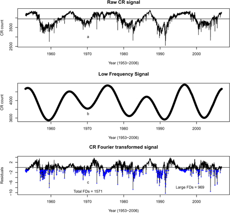
Figure 1. (a) Raw CR daily data; (b) slow-moving signal part of panel (a); (c) high-frequency signal part of panel (a). Blue stars indicate FD dates and magnitudes.
Download figure:
Standard image High-resolution image6. Results and Discussions
6.1. Algorithm to Select FDs
The blue stars in Figure 1(c) represent the dates as well as the FD magnitudes for the whole period (54 yr) that Climax Observatory has data. While it might be easier to manually detect FDs in CR data spanning a period of a few years, FD manual identification might be intractable given the large volume of CR data as presented in Figure 1(a). In order to amplify the clustered stars for easy comparison with the results of other investigators, we split Figure 1(c) into three, presented in Figures 2–4.
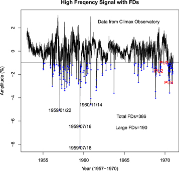
Figure 2. Same as Figure 1(c), but for 1957–1970.
Download figure:
Standard image High-resolution image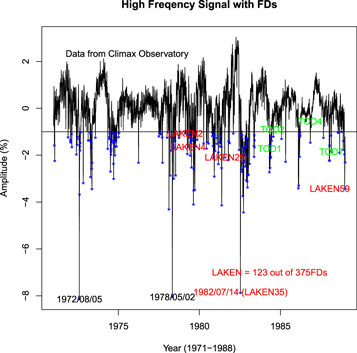
Figure 3. Same as Figure 1(c), but for 1971–1988.
Download figure:
Standard image High-resolution image6.1.1. Result Validation/Strong FDs
1. Comparison with IZMIRAN catalog: Our program detected a total of 1571 FDs for the period 1957–2006 using daily CR data, while Belov’s group, which produces the IZMIRAN FD catalog (http://spaceweather.IZMIRAN.ru/eng/dbs.html), calculated a total of 6060 FDs within the same period. A baseline of CR(%) ≤ 0.5 is used for the selection of the 1571 FDs, whereas CR(%) ≤ 1 is used for the 969 large FDs selected within the period. The IZMIRAN FDs are based on hourly data and the dates defined by FD onset, whereas the FD dates indicated in Figure 1(c) are defined by the largest depression in CR flux.
When we investigated hourly data, our program detected a total of 2139 FD events with CR(%) ≤ −3.5 baseline. The increased baseline is in line with the submission of Lockwood (1971) that the ratio of the magnitude of the decrease for a few hours could be about 2:1 when compared with the daily average at any cutoff rigidity; our program uses larger baselines for hourly data than when daily averages are analyzed. When we vary the baseline following Okike & Umahi (2019b), baselines of CR(%) ≤ −3 and CR (%) ≤ −2.5 detected 3905 and 6797 FDs, respectively.
Although the group uses a more accurate event selection approach and CR data from the worldwide NMs (Belov et al. 2005), involving CR physical characteristics such as CR density and anisotropy, Okike & Umahi (2019b) observed that their method and FD data are not widely used by researchers analyzing solar–terrestrial connections (see Section 3 for various techniques common among FD-related studies). The notable large FD event of 2005 January 19 frequently used in many superposition investigations (e.g., Svensmark et al. 2016), for example, was recorded on 2005 January 18 in their list.
2. Strong FDs: The magnitude of FDs, as well as what determines it, has been a subject of interest among CR researchers (see Belov et al. 2001). Traditionally, the magnitude of an event usually expressed as a percentage is an indicator of the size or strength of the event. This quantity depends on a number of variables (e.g., the type of CR monitor, vertical cutoff rigidity, and the detector’s atmospheric depth) and should have unique values for specific locations on Earth. However, a survey of literature shows that for a certain place on Earth, different publications might calculate different values for the same FD event using the same NM data. The magnitude of the largest FD event of 1991 June 13 was calculated as 30% and 7% by two different authors using the same CR data (see Paper II for details).
In a bid to further the investigation on FD magnitude/strength and its implication on atmospheric ionization, some researchers (see Usoskin et al. 2011; Svensmark et al. 2016) attempt to rank FDs and GLEs. Svensmark et al. (2009b) presented FDs ranked according to their impact on the low-altitude atmosphere. The same approach is adopted in Svensmark et al. (2012, 2016). Although ranking of FDs requires assimilation and analyses of all the NM data (a task we will leave for future work) as demonstrated by the IZMIRAN group, it might be interesting to compare the results of Svensmark et al. (2016) and a few other published FDs with our result.
Figures 2–4 are presented for the purpose of such comparisons. The symbols PU1, PU2, ..., LAKEN1, LAKEN2, ..., TOD1, TOD2, ..., CA1, CA2, ..., A1, A2, SV1, SV2, ..., and S1, S2, ..., indicated in Figures 2–4, respectively, stand for FDs taken from the lists of Pudovkin & Veretenenko (1995), Laken et al. (2011), Todd & Kniveton (2001), Calogovic et al. (2010), Ahluwalia et al. (2009), and Svensmark et al. (2012, 2016). Except for PUs in Figure 2 where orders 1, 2, and 3 represent serial number of FDs in the list, the rest denote the magnitude/strength of the events in the respective articles. We note that comparison of FDs requires that the same NM data as those of the publications referred be used. However, Oh et al. (2008) and Paper II showed that strong FDs are global phenomena observed simultaneously at all points on Earth. Such large events are generally selected by investigators searching for solar–terrestrial linkage. Before taking up some case studies where the same CR data are used for comparisons, the strong FD events from the papers referred above are compared with the results obtained using Climax data. Three events PU2–PU4, corresponding to the events of 1969 March 24, 1969 November 9, and 1970 June 18, are shown in their Table 1. The first event in their list (PU1, 1969 March 17) might be a small and nonsimultaneous event, as it was not observed at the Climax station. Pudovkin & Veretenenko (1995) assigned 4.8%, 4.5%, and 2.9% to PU2–PU4, respectively, while the corresponding magnitudes calculated for the events by our program are 1.7%, 0.99%, and 2.7%. Though the difference in sizes of FDs might be attributed to the differences in the FD selection method and/or the differences in cutoff rigidity between the two CR stations (Apatity and Climax), it can be inferred that these three events are strong and hence simultaneous at the two NMs. The number of FDs ≤0.99% between 1969 and 1986 is 519. Except for another selection criterion (exclusion of FDs occurring within the time of solar proton events) imposed by Pudovkin & Veretenenko (1995), the implication of this result is that they analyzed about 13% of the strong FDs that could be investigated within the same period using Climax data. The relative strengths of FDs for the period 1957–1970, as well as the total FDs and the number of strong FDs, are shown in Figure 2. In decreasing order of strength, the four largest FDs happened at 1959 July 18, 1959 July 16, 1959 January 22, and 1960 November 14.
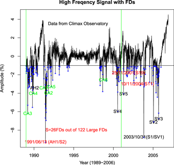
Figure 4. Same as Figure 1(c), but for 1989–2006.
Download figure:
Standard image High-resolution imageLaken et al. (2011) used a comparatively larger number of strong FDs (123). Some of the events are indicated in Figure 3 for illustrative purposes. Judging by the magnitude (−1.07%) of the least event (LAKEN2) in the diagram, the number of events within their period (1978–2006) of investigation is 375. The event of 1982 July 14 is the largest in their least. This also confirmed in Figure 3. Two other large events (1972 August 5 and 1978 May 2) are also conspicuous in the diagram. We note that they did not identify their FD onset date from any particular NM data. Their events dates were rather selected from various sources (e.g., published articles, online website).
Some of the events identified by Todd & Kniveton (2001) are marked in Figure 3. Although they claimed to use large FDs, Figure 3 shows that some of the events they used might be quite small. TOD4, for example, is the event of 1986 November 3. They assigned a magnitude of 4.1% to the event, whereas our program calculated the magnitude of the same FD as 0.55%. TOD2 is also a small event (appearing above the horizontal line in the diagram).
A number of strong FDs reported in the other four papers are indicated in Figure 4. While the magnitudes of AH and CA can be interpreted in light of Figures 1 and 2, the events represented by S and SV are selected by Svensmark et al. (2012, 2016) using a system of FD ranking. Some of these events are displayed here to test the agreement between their method of FD ranking and our approach to calculation of FD magnitudes. SV1–SV5 suggest a good agreement between their ranking method and our event catalog. The same applies to the events represented by S. Except for the event of 1991 June 13, which is strongest in Figure 4 but ranked second to that of 2003 October 31 by Svensmark et al. (2016), the order of strength of S11 and S19 is in line with their ranking. The magnitude of the event on 2001 November 25 (S19) is 1.82%, whereas Svensmark et al. (2016) assign it a magnitude of 39%. The number of FDs ≥ 1.82% between 1987 and 2006 is 122, implying that they investigated about 21% of the strong events that happened within the period.
6.2. Case Studies
6.2.1. Pudovkin & Veretenenko (1995)
Although the illustration in the preceding section might have reasonably highlighted the existing gap in the FD key event data selection criteria, timing, and ranking when conducting a Chree analysis, one may argue that some of the glaring differences in the number of FDs selected by the literature referred above and the number selected by our programs could rather be attributed to the type of NM data used. The argument is sound since the characteristics of CR detectors vary widely, coupled with the nonuniform distribution of GCRs over Earth, as well as varying cutoff rigidity (Papers II and III). Pudovkin & Veretenenko (1995), for example, analyzed CR data from the Apatity CR station, whereas Climax data are used in the result presented in Figure 2. Figure 5(a) shows data from the Apatity CR station, while Figure 5(b) shows one of the harmonics of interest. The dates/magnitudes of the three conspicuous events ranked according to their strength from the strongest to the weakest are (1978 May 2)/FD1 (134%), (1982 July 14)/FD2 (132%), and (1972 August 5)/FD3 (130%). It can be observed that these three events are also reflected in Figure 5(b), confirming the sinusoidal fidelity of the present technique. Inspection of their FD list in their appendix shows that these three main events are not included. The increasing order of the strength of the event they selected is denoted with the symbols PU1, PU2, PU3, ..., PU65, with PU65 standing for the weakest event included in the appendix referred.
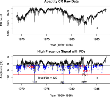
Figure 5. High-frequency signal (Apatity), with stars representing FDs.
Download figure:
Standard image High-resolution imageBeyond the three largest events, PU1 is the fourth-largest FD as measured by the red horizontal line. There are, however, many other events with similar magnitudes to PU1 that were not identified by their method. PU2 is much smaller than many other FDs that are not selected. The order of their FD magnitude also does not agree with ours, as it is evident that PU15 is much stronger than PU3. While our code tracked most of their events, a number of their events (e.g., 1973 July 26, 1973 January 9, 1973 September 22, 1973 October 31, 1976 March 30) are not reflected in Figure 5(b). A close inspection of their list reveals that these are among the smallest events they identified. As hinted at earlier, attempts to select low-magnitude FDs manually would be biased by CR diurnal anisotropy if not first isolated as illustrated by Paper III. Out of the 422 large FDs selected by our program for the years 1969–1986, Pudovkin & Veretenenko (1995) identified 65 (about 15%) events. However, they noted that Forbush events superposed in the first 3 days by solar proton events are purposefully excluded in their list. But McCracken (2007) indicated that SEPs occur rarely, so as to justify the exclusion of 85% of the FDs within the same period. Asvestari et al. (2017) had a list of the 16 GLEs recorded by the NM for the 18 yr period. This translates to 0.89 yr−1 and 4% of the large FDs within the period. For the years 1958–2005, they estimated the annual frequency of occurrence of such events as 0.06 yr−1, though Todd & Kniveton (2001) indicated that there are years when it might occur once or even as high as 8 yr−1 in some cases.
Figure 5 (Apatity) indicates that a total of 422 large FDs are detected between 1969 and 1986, whereas 519 strong events are reported when Climax data were analyzed for the same period (Figure 1(a)). In addition to the difference in the number of years used for the two figures, the differences might be attributed to cutoff rigidity between the two stations. In order to illustrate the implication of choice of normalization period on the number of FDs selected within a given time, we included more years in Apatity data. When data between 1961 and 2016 were used, a total of 555 FDs were picked for the same period 1969–1986. The mean CR count for the longer period 1961–2016 (7431.741) is larger than that of 1969–1986 (7431.031), and since our program normalizes CR to the mean value of the period used, a greater number of FDs are selected between 1969 and 1986 when a longer data time series is used. This could also explain the fewer number of events detected by researchers using a few-days running mean as a reference point (see Okike & Umahi 2019b, for details of other factors that determine the number of FDs selected with given CR data).
6.2.2. Laken et al. (2011)
The solar–terrestrial analysis of Laken et al. is both unique and controversial. The number of FDs (123; see their Figure 1) used in the study is much larger than those of previous studies. This should, in principle, solve the problems of small sample size and low signal-to-noise ratio that were earlier neglected. In spite of their tremendous efforts to increase FD sample size, they could not confirm the CR–cloud link. Rather, anomalous cloud changes over the Antarctic plateau, believed to be induced by GCRs, were blamed on solar irradiance. In light of the present work, their methodological approach recommends itself for a reassessment.
Their events were selected from different sources, including literature and websites, for the period 1978–2006. Selecting up to 123 FD key times manually is an onerous task, considering the high variability and hidden periodicities in the CR flux. Although FD key dates have previously been accepted without validation, Okike & Umahi (2019b) recently noticed the need for correct and careful selection and timing of Forbush events. One of the ways of validating key event dates selected for a Chree analysis is demonstrated by Harrison & Ambaum (2010). Following the same method, we present some events in the list of Laken et al. (2011) in Figure 6. The green line with filled circles is the mean. While big FDs can be manually selected without much bias, attempts to select small FDs could be frustrated by the presence of CR anisotropy. A comparison of Figures 6 and 1 of Harrison & Ambaum (2010) would suggest that most of the events in Figure 6 are not FDs. Laken et al. (2011) presented an interesting result of the average of all 123 FDs in their Figure 2(a). Again, a comparison of their Figure 2(a) with some of the individual cases in Figure 6 reveals a bias problem in their technique. If a reasonable number of events in their list are not FDs as is reflected in Figure 6, how does the composite mean in their Figure 2(a) exhibit the sudden depression, maximal depression, and slow recovery characteristics of FDs? We have a similar case in Figure 6. Instead of maximal reduction on the epoch day, some of the events show increases, with some recording maximum depression several days after the key date. These notwithstanding, the mean apparently looks like an FD, though the distinctive features are missing. This is attributable to leveraging, one of the unsolved problems in the Chree method (Okike & Umahi 2019b) of investigation, as we will shortly demonstrate.
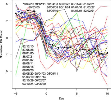
Figure 6. Validating FD key dates in the list of Laken et al. (2011).
Download figure:
Standard image High-resolution imageFigure 7 is presented to show the influence of a single large anomaly on the results of a Chree analysis. It is easy to see that four of the events are not only real but also the strongest FDs in their list, while four events, marked with dashed lines, are probably not FDs, as some of them have their minimum 10 days after the epoch day. Since the SEA method is vulnerable to leveraging that can result from the influence of one or more large anomalies, the mean signal in Figure 7 is weighted toward the large FD values. Okike & Umahi (2019b) suggested that the problem of leveraging can be solved by increasing the sample size or by including the normalization step in superposition analysis, while Laken et al. (2012) concluded that some normalization procedures may result in false positives in an SEA as illustrated in Figures 6 and 7.
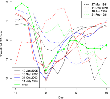
Figure 7. Illustration of leveraging problem in composition analysis.
Download figure:
Standard image High-resolution imageThough their sample size was significantly increased compared to other reports that used as few as six FDs, 123 FDs, selected for their investigation within a 29 yr period, might look very small. The result presented in Figure 1(b) covers the same duration. The number of large Forbush events selected by our program for the years 1978–2006 is 522, implying that only 23% of the strong FDs that occurred within the time were considered in their analysis. We observe, however, that these numbers will vary between CR stations.
6.2.3. Kristjansson et al. (2008)
This work is a little different from those considered earlier. They selected 22 FDs from the Climax station for the years 2000–2005 and went ahead to validate their results using FDs selected from two other stations, Oulu and Moscow NMs. Events observed simultaneously by the three stations should be strong and global (Oh et al. 2008, Paper II). But selecting FDs visually from three stations is subject to bias, among other limitations. Due to nonuniform distribution of GCRs over Earth, the number of FDs seen by one station may differ significantly from those of other stations. This is because CR intensity variability manifests both longitudinal and latitudinal dependence (Tezari et al. 2016; Okike & Umahi 2019b). FD detection, especially small FDs, requires averaging over a number of stations (Barouch & Burlaga 1975), rather than a filtering method. Assimilating data from a number of CR stations requires empirical orthogonal function analysis to extract the leading principal components (see Paper II for details of the methodology). Figure 8(a) represents the PC1 signal resulting from three CR stations (Climax, Oulu, and Moscow). The correlation coefficient between PC1 loadings and PC1 scores is ≈99 for each of the stations. The high correlation coefficients suggest that PC1 accounts for all the intensity variations in the three stations. The proportion of variance due to PC1 is ≈98%, while PC2 and PC3 account for the remaining 2%.
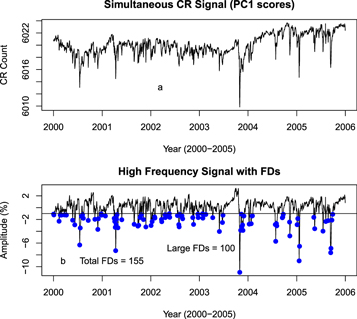
Figure 8. (a) Simultaneous CR signal (PC1 scores) for 2000–2005. (b) High frequency of PC1 with FDs.
Download figure:
Standard image High-resolution imageFigure 8(b) is the high-frequency signal containing the high-magnitude FDs. The number of large events detected using a baseline of CR(%) ≤ −1 is 100. Although this numerical averaging over a number of stations is more involved (Barouch & Burlaga 1975, Paper II) than filtering over a single station, it is a unique tool for isolating strong/global FDs than the usual FD magnitude, which varies across Earth. All the FDs as reflected in Figure 8 are strong and simultaneous at the three stations, while the local variations that are station dependent, such as weak or nonsimultaneous FDs, are averaged out (Haurwitz & Brier 1981; Okike & Umahi 2019b). In light of the presented PCA analysis, simultaneity of FD event is a stronger indicator of the strength of Forbush events than the percentage decreases, which vary among authors and between places on Earth. Detailed explanation of the usefulness of this approach, especially with regard to weak and strong Forbush event discrimination in a Chree analysis, is left for future work. We, however, note in brief that Kristjansson et al. (2008) admitted that only 6 out of the 22 FDs selected for their analysis were strong, whereas Figure 8 shows that a larger number of big FDs are observed between 2000 and 2005. Indeed, the period 2000–2005 falls within the time of high solar activity as can be inferred from Figure 8(b). The 22 FDs investigated by Kristjansson et al. (2008) imply using only 22%/15% of the large/total FDs in comparison with the number selected by our algorithms. The authors agreed that their failure to see any clear FD-low cloud connection could be due to the small FD sample employed in their analysis. A larger number of key event times is thus required to confirm their result.
6.3. Summary and Conclusions
A review of Schuurmans & Oort (1969) and Pittocks (1978) indicates that very many scientists, especially the meteorologists, have been highly critical of the empirical results on solar–terrestrial relationships. Statistical significance tests of epoch results, data selection/quality, data smoothing, and autocorrelation issues are some of the initial sources of doubt on solar–terrestrial analysis. Schuurmans & Oort (1969) responded early to the questions regarding suitability of statistical tests. Haurwitz & Brier (1981) and Forbush et al. (1982a) adopted a different approach to demonstrate the nonapplicability of the traditional t- F-, or p-values in the significant test of epoch results. Several years after its introduction, there seems to be a renewed interest (see Laken & Calogovic 2013; Scott et al. 2014; Paper III) in the statistical method of Schuurmans & Oort (1969), which accounts for the presence of autocorrelation in geophysical data. The detailed illustration of Laken & Calogovic (2013) not only redirected researchers to the correct method of statistical significant test but also tends to lay the age-long problems of incorrect test of significance attendant on solar–terrestrial connection to rest.
However, data selection and smoothing/filtering are yet to be fully considered. This is partly because many solar–terrestrial investigators presume that data selection, for instance, is a preliminary stage that does not require much attention. Another reason, as observed by Shea & Smart (2000), could be due to the fact that some researchers investigating solar–terrestrial links, for example, are not familiar with solar physics and CR topics. Nevertheless, the highly critical work of Pittocks (1978) confirms that adequate attention should be given to event selection. The publication has a long list of authors that dubiously selected data to suit their preconceived results.
In light of these criticisms, the present work attempts to call the attention of investigators conducting SEA studies with the FDs and employing regression analysis to test various solar–terrestrial connections to the need for a detailed and careful method of FD event selection. Ramirez et al. (2013) found that FD is the most spectacular variability in the GCR flux and, as such, accurate detection of Forbus events in a large volume of CR data requires a sophisticated method as opposed to the simple (manual) technique documented in numerous studies (Harrison & Ambaum 2010; Laken et al. 2011). Such careful and accurate methods (e.g., ring station method, global survey method) were first developed by the IZMIRAN group (Kudela et al. 2000; Belov et al. 2001, 2005; Belov 2008), and their FDs have been used in several solar–terrestrial studies (see, e.g., Belov et al. 2001; Belov 2008). While they identified 5900 FDs between 1957 and 2006, for example, Harrison & Ambaum (2010) selected 137 FDs even in a longer period (1952–2006) using the manual method of plotting and calculating the amplitude of each event. A comparison of the large number of FDs identified and used by the IZMIRAN group with the small number of FDs selected by other researchers reveals the pitfalls associated with manual FD event selection. The presented harmonic transformation and the accompanying R program tend to lend credence to the abundance of large FDs as demonstrated by the IZMIRAN global survey method (Belov et al. 2001, 2005). While their method uses FD onset time, our program is based on the time of maximal depression. The large event of 2003 October 31 is, for instance, recorded from 2003 October 28 to 30, with the largest magnitude (29.7%) on 2003 October 29, at the IZMIRAN website. Again, a survey of literature shows that the time of maximal CR reduction, rather than the onset time, is more frequently used in composition analysis (Laken et al. 2011; Svensmark et al. 2012), implying that FDs selected by the present algorithm might attract the attention of solar–terrestrial physicists conducting FD-related Chree analysis.
A note of caution is, however, in place here. FD is such a complex phenomenon that no single algorithm or software can completely account for the physics and knowledge behind it. Although substantial efforts are being usually made by the principal investigator that prepares CR data, Shea & Smart (2000) found that CR data are not always completely without errors. It is thus speculated that some of the events picked by our program could be outliers or other erroneous data arising from data handling. In light of this, the present analysis can serve as a stepping stone to accurate FD identification. In particular, events selected by our program could further be validated with solar wind and interplanetary data corresponding to the calculated event time. Additionally, while our program calculates FD event time and magnitude with great precision, it is incapable of describing the nature of the onset, main phase, or recovery phase of a Forbush event. Thus, an investigator interested in separating different types of FDs can use the key time detected by our program and then plot the data so as to visualize whether a particular event has sudden or slow onset, fast or slow recovery phase, and so on.
The current analysis reconfirms the indication of Okike & Umahi (2019b) that there are several factors that could influence the number and size of FDs identified for a given CR data. One such factor, commonly considered by CR scientists, are pre-defined baselines. Using a baseline of ≥3 (Laken et al. 2011) or ≥5 (Kristjansson et al. 2008), researchers hope to select large or strongest FDs and thus assign event sizes. Kristjansson et al. (2008), for instance, calculated 22% reduction for the event of 2003 October 31. However, the automated method uses a smaller baseline of order 0.5 (for smaller FDs) or 1 (strong events). Figure 1(c) also shows that our program assigns a much smaller percentage reduction to FDs, though the differences in the CRA data temporal resolutions per day, hour, minute, or second also play a significant role in the assignment of FD sizes (Lockwood 1971). The event of 2003 October 31 is 8.8% (Figure 4). While the magnitude of the largest event of 1991 June 13 was calculated as −30% and −7%, respectively, by Gurnett & Kurth (1995) and Ahluwalia et al. (2009), Figure 4 suggests that the magnitude is about 9%. Thus, baselines and FD magnitudes are relative quantities that might assume different values for different researchers/algorithms even for the same FD event. Uniqueness can only be assigned globally to date or time of maximum reduction (onset time may not be the same/simultaneous even for strong events) of FDs, provided that they are simultaneous and strong events. This is also why several investigators use date of maximal depression for SEA studies. The situation is different for weak FDs as is also illustrated by the figures in Paper II.
The result presented in Figure 8 is a preliminary test of FD ranking by our algorithm. Three CR stations are employed here. If all the CR NM data are included in the PCA analysis as attempted by Paper II or the global survey method of Belov’s group, a complete FD ranking catalog might be created. The catalog could account for all the strong and simultaneous Forbush events that have occurred since continuous monitoring of CR flux began. Such a list of large FDs might be useful for investigating the age-long controversial solar–terrestrial relationships.
The road maps defined by the referee of the present manuscript have further convinced us that the level of criticism determines the quality of any scholarly work. While we had several competing but uncoordinated ideas at the beginning of the submission, a few iterations between us and the reviewer streamlined the work, and we became much more focused. We are thus honestly indebted to the interested and committed anonymous reviewer. We did not have to purchase the data used in the present analysis, as they were freely downloaded from http://cr0.izmiran.ru/common/links.htm. The groups maintaining the website are gratefully acknowledged.