Abstract
Zirconium oxide (ZrO) is an important astrophysical molecule that defines the S-star classification class for cool giant stars. Accurate, empirical rovibronic energy levels, with associated labels and uncertainties, are reported for nine low-lying electronic states of the diatomic  molecule. These 8088 empirical energy levels are determined using the Measured Active Rotational-Vibrational Energy Levels algorithm with 23,317 input assigned transition frequencies, 22,549 of which were validated during this study. A temperature-dependent partition function is presented alongside updated spectroscopic constants for the nine low-lying electronic states.
Original content from this work may be used under the terms of the Creative Commons Attribution 3.0 licence. Any further distribution of this work must maintain attribution to the author(s) and the title of the work, journal citation and DOI.
1. Introduction
ZrO is a transition metal diatomic oxide that, like similar species, possesses strong absorption lines and a complex electronic structure. Strong ZrO absorption lines are the identifying characteristic of the rare S-type stars (Merrill 1922; Keenan 1954; Wyckoff & Clegg 1978; Ake 1979; Keenan & Boeshaar 1980; Little-Marenin & Little 1988; Van Eck & Jorissen 2000). Traditionally thought to be caused by carbon/oxygen ratios near unity (Ake 1979; Smith & Lambert 1986), the recent investigation by Van Eck et al. (2017) confirms the earlier claim by Piccirillo (1980) that the ZrO lines are caused by the overabundance of slow neutron-capture process (s-process) elements like Zr. Weak ZrO bands are characteristic of SC stars (Keenan & Boeshaar 1980; Zijlstra et al. 2004). Faint ZrO bands have also been identified in sunspots (Richardson 1931; Sriramachandran & Shanmugavel 2012) and M-stars (Bobrovnikoff 1934).
The ZrO absorption bands were first observed in spectra taken by Merrill (1922), with King (1924) providing laboratory confirmation of the molecular origin of the bands. Keenan (1954) provided the first classification of S-type stars. Early studies of ZrO bands in stars include an analysis of R Geminorum by Phillips (1955).
The presence of ZrO (and molecules formed by other s-process elements) in S-stars is due to the nucleosynthesis s-process occurring within these stars (Joyce et al. 1998) or in a companion star before being accreted to their surface (Van Eck & Jorissen 2000). The s-process only occurs at relatively low neutron densities and intermediate temperature conditions. There are two types of S-stars depending on whether the s-process elements are formed within the star itself or transferred from a binary partner star. Short-lived cooler intrinsic S-stars are formed in around 10% of asymptotic giant branch stars (AGB) when s-process elements convect to the surface due to dredge-up during the short thermal pulse-AGB phase (Smith & Lambert 1985; Van Eck & Jorissen 2000). Longer-lived hotter extrinsic stars are formed due to binary system mass transfer (Lambert et al. 1995; Van Eck & Jorissen 2000), and are evolutionarily understood as the descendants of barium stars (Van Eck & Jorissen 2000). They can be distinguished by the presence of Tc in intrinsic S-stars (Van Eck & Jorissen 1999, 2000; Van Eck et al. 2000).
Littleton & Davis (1985) are regularly cited as providing 330,000 lines of a ZrO line list; however, these data are not available as part of the original publication. It is likely this cited line list consists of model Hamiltonian fits to the main bands along with band intensities, Franck–Condon and Hönl–London factors. This has been superseded by the line list created using similar methods by Plez et al. (2003), which is unpublished but freely available online. There is thus, to our knowledge, no available line list created using variational nuclear-motion methods from fitted potential energy, ab initio dipole moment, and fitted spin–orbit coupling curves, as can be constructed using current techniques by, e.g., the ExoMol group (Tennyson & Yurchenko 2017). Such studies are greatly aided by the availability of accurate empirical energy levels such as the data set developed in this paper.
Due to its astrophysical importance, ZrO has been the subject of a large number of experimental studies. One of the aims of this paper is to review and compile the spectroscopic data from these previous studies to produce a single recommended list of experimentally derived empirical energy levels and validated transition frequencies. As part of this process, we extracted all previous experimental data into a consistent set of assigned transition frequencies with uncertainties. Future experimental results can be added to this Master List to obtain an updated list of empirical energy levels using the Measured Active RoVibrational Energy Levels (Marvel) program (referenced and described below). We anticipate that these energy levels will be used to refine new spectroscopic models for  and produce updated extensive hot molecular line lists for use in atmospheric models.
2. Method
2.1. Marvel
The Marvel approach (Császár et al. 2007; Furtenbacher et al. 2007; Furtenbacher & Császár 2012a) is an algorithm that enables a set of assigned experimental transition frequencies to be converted into empirical energy levels with associated uncertainties propagated from the input transition data to the output energy levels. This conversion relies on the construction of experimental spectroscopic networks (SNs; Császár & Furtenbacher 2011; Furtenbacher & Császár 2012b; Furtenbacher et al. 2014; Árendás et al. 2016) which contains all interconnected transitions. For a detailed description of the approach, algorithm, and program, we refer readers to Furtenbacher & Császár (2012a).
The Marvel approach has been used to compile empirical energy levels for the very important and electronically similar species48Ti16O (McKemmish et al. 2017). Other Marvel studies on astronomically important molecules include those for  (Furtenbacher et al. 2016), acetylene (Chubb et al. 2018a), ammonia (Al Derzi et al. 2015; Furtenbacher et al. 2018), SO2 (Tóbiás et al. 2018), H2S (Chubb et al. 2018b), and isotopologues of
  (Furtenbacher et al. 2013a, 2013b). These are in addition to energies for the isotopologues of water (Tennyson et al. 2009, 2010, 2013, 2014b) for which the MARVEL procedure was originally developed (Tennyson et al. 2014a).
This paper utilized the Marvel algorithm through a specially designed web interface, available at http://kkrk.chem.elte.hu/marvelonline (Furtenbacher & Császár 2018), making it highly accessible across computer systems without installation of a specialized code. Numerous updates to the online interface were also made during this project and related projects in order to optimize the speed, ease, and quality of data processing; for example, options were made available to automatically update uncertainties within thresholds when processing initial data to find a self-consistent SN.
2.2. Electronic Structure and Spectroscopy of ZrO
ZrO and TiO share similar features in their electronic structure, as Zr is directly below Ti on the periodic table. Specifically, both have the same qualitative ordering of many low-lying electronic states (in terms of symmetry and spin), with slight differences in Te so that, e.g., unlike in TiO, the ground electronic state of ZrO is a spin singlet,  . Those states with well-characterized experimental electronic states below 25,000 cm−1 are shown in Figure 1, which also gives the observed bands linking these states. Note that we did not find any rotationally resolved spectral data involving the
  ,
,  ,
,  , or
, or  states.
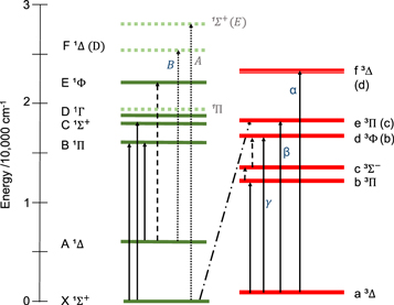
Figure 1. Electronic states of  , with approximate Te and labels taken from Langhoff & Bauschlicher (1990); where different, labels from Huber & Herzberg (1979) are given in brackets. The solid horizontal lines are those electronic states whose existence and assignment is reasonably secure with reliable theoretical predictions, while the dashed horizontal lines indicate states that some authors have proposed for ZrO but that are not supported by theory or rotationally resolved experiment. This diagram also shows the main band systems of ZrO, with solid lines showing the bands for which rotationally resolved allowed transitions have been analyzed, the alternating dotted–dashed line representing an experimentally observed intercombination band while long dashed lines represent allowed transitions that have not been measured in rotationally resolved spectra and the short dashed lines represent transitions that have previously, probably erroneously, been assigned as ZrO bands.
Download figure:
Standard image High-resolution imageThe singlet  ground state has allowed excitations to the
  and
and  states. Significant absorption also occurs from thermal population of the
  states to the higher singlet states
  ,
,  ,
,  , and
, and  . In the high temperature gaseous environments where
  is present astrophysically, transitions from the
  state to the
  and
and  states may also be relevant.
2.3. Quantum Numbers and Selection Rules
The most obvious information to include in the label of a rovibronic state of ZrO is the electronic state, state, the total angular momentum, J, and the vibrational quantum number, v. We find these to be relatively unambiguous to define.
For the triplet states, we also need to provide information about the electronic spin state; in this case, we choose to include this as part of the label for the electronic state. The parity of energy levels usually only influences the energy in a measurable manner for Π states; we absorb the e and f parity labels (Brown et al. 1975) into the electronic state label to reduce the overall number of labels.
2.4. Literature Review
In the first half of the twentieth century, there was considerable interest in studying the visible and ultraviolet spectrum of  , with many bandheads measured by Lowater (1932), Herbig (1949), and Afaf (1949, 1950a, 1950b). These studies include many involving transitions to electronic states that have yet to be investigated using rotationally resolved spectra.
More recently, there was an extensive experimental effort over the 1970s to early 1980s by several groups to obtain rotationally resolved assigned experimental spectra for various important  bands; these studies as well as more recent rotationally resolved studies are summarized in Table 1.
Table 1.
Data Sources and Their Characteristics for 
| Tag | References | Band | Range (cm−1) | J Range | Trans. (A/V) | Uncertainties (cm−1) | |||
|---|---|---|---|---|---|---|---|---|---|
| Min | Av | Max | |||||||
| 54LaUhBa | Lagerqvist et al. (1954) |
 2– 2– 1 1 |
0–0 | 15282–15442 | 11–89 | 159/159 | 0.1 | 0.1 | 0.28 |
 3– 3– 2 2 |
0–0 | 15612–15755 | 11–93 | 149/149 | 0.1 | 0.1 | 0.32 | ||
 4– 4– 3 3 |
0–0 | 15898–16048 | 11–95 | 165/165 | 0.1 | 0.11 | 0.34 | ||
 1– 1– 1 1 |
0–0 | 21351–21542 | 20–76 | 105/105 | 0.1 | 0.1 | 0.31 | ||
 2– 2– 2 2 |
0–0 | 21351–21555 | 20–80 | 111/111 | 0.1 | 0.1 | 0.1 | ||
 3– 3– 3 3 |
0–0 | 21457–21640 | 20–81 | 106/106 | 0.1 | 0.1 | 0.1 | ||
| 54Uhler | Uhler (1954b) |
 0e– 0e– 1 1 |
0–0 | 17884–18002 | 15–60 | 106/106 | 0.1 | 0.1 | 0.14 |
 0f– 0f– 1 1 |
0–0 | 17889–18006 | 27–59 | 96/91 | 0.1 | 0.1 | 0.3 | ||
 1e– 1e– 2 2 |
0–0 | 17619–17757 | 20–74 | 103/91 | 0.1 | 0.12 | 0.31 | ||
 1f– 1f– 2 2 |
0–0 | 17653–17758 | 19–59 | 99/63 | 0.1 | 0.19 | 0.62 | ||
 2– 2– 3 3 |
0–0 | 17326–17483 | 13–85 | 143/139 | 0.1 | 0.15 | 0.43 | ||
| 57Akerlind | Akerlind (1957) |
 – –
|
0–0 | 18994–19280 | 17–102 | 156/156 | 0.1 | 0.1 | 0.11 |
 – –
|
1–0 | 19843–20106 | 35–94 | 110/110 | 0.1 | 0.1 | 0.15 | ||
| 73BaTa | Balfour & Tatum (1973) |
 e– e–
|
0–0 | 15136–15391 | 18–107 | 149/145 | 0.01 | 0.031 | 0.16 |
 f– f–
|
0–0 | 15185–15382 | 8–96 | 85/83 | 0.01 | 0.024 | 0.13 | ||
| 73Lindgren | Lindgren (1973) |
 1e– 1e– 1 1 |
0–0 | 17995–18050 | 30–61 | 53/53 | 0.07 | 0.086 | 0.19 |
 1f– 1f– 1 1 |
0–0 | 17991–18048 | 30–60 | 51/50 | 0.07 | 0.09 | 0.23 | ||
 2– 2– 2 2 |
0–0 | 17761–17820 | 47–65 | 36/29 | 0.07 | 0.12 | 0.35 | ||
| 76PhDa.CX | Phillips & Davis (1976a) |
 – –
|
0–0 | 16732–17060 | 2–121 | 232/203 | 0.02 | 0.044 | 0.19 |
| 76PhDa.BX | Phillips & Davis (1976b) |
 e– e–
|
0–0 | 15102–15391 | 5–132 | 201/188 | 0.02 | 0.039 | 0.14 |
 e– e–
|
0–1 | 14292–14423 | 1–102 | 144/135 | 0.02 | 0.046 | 0.18 | ||
 e– e–
|
0–2 | 13244–13431 | 17–116 | 101/100 | 0.02 | 0.042 | 0.1 | ||
 e– e–
|
1–0 | 16023–16244 | 1–107 | 149/148 | 0.02 | 0.046 | 0.16 | ||
 e– e–
|
1–2 | 14038–14313 | 4–116 | 177/175 | 0.02 | 0.045 | 0.31 | ||
 e– e–
|
1–3 | 13246–13359 | 1–102 | 135/134 | 0.02 | 0.042 | 0.15 | ||
 e– e–
|
2–0 | 16817–17091 | 4–117 | 159/142 | 0.02 | 0.056 | 0.2 | ||
 e– e–
|
2–1 | 15936–16122 | 1–104 | 146/136 | 0.02 | 0.046 | 0.27 | ||
 e– e–
|
2–3 | 14046–14205 | 1–106 | 136/135 | 0.02 | 0.048 | 0.17 | ||
 e– e–
|
2–4 | 13122–13257 | 2–108 | 150/147 | 0.02 | 0.034 | 0.14 | ||
 e– e–
|
3–1 | 16690–16963 | 1–90 | 114/111 | 0.02 | 0.038 | 0.14 | ||
 e– e–
|
3–5 | 13051–13157 | 1–100 | 135/132 | 0.02 | 0.036 | 0.24 | ||
 e– e–
|
3–6 | 11990–12223 | 1–136 | 188/185 | 0.02 | 0.036 | 0.15 | ||
 e– e–
|
4–2 | 16547–16836 | 2–116 | 139/139 | 0.02 | 0.04 | 0.3 | ||
 e– e–
|
4–5 | 13746–13991 | 1–104 | 102/100 | 0.02 | 0.043 | 0.3 | ||
 e– e–
|
4–6 | 12824–13057 | 2–108 | 132/132 | 0.02 | 0.042 | 0.22 | ||
 e– e–
|
5–3 | 16659–16710 | 2–61 | 46/46 | 0.02 | 0.029 | 0.064 | ||
 e– e–
|
5–7 | 12822–12959 | 2–108 | 130/130 | 0.02 | 0.026 | 0.13 | ||
 f– f–
|
0–0 | 15108–15383 | 1–113 | 114/109 | 0.02 | 0.036 | 0.17 | ||
 f– f–
|
0–1 | 14289–14414 | 2–80 | 77/73 | 0.02 | 0.047 | 0.44 | ||
 f– f–
|
0–2 | 13250–13431 | 34–107 | 70/70 | 0.02 | 0.034 | 0.14 | ||
 f– f–
|
1–0 | 16021–16237 | 1–96 | 93/93 | 0.02 | 0.037 | 0.1 | ||
 f– f–
|
1–3 | 13248–13349 | 3–76 | 72/72 | 0.02 | 0.036 | 0.16 | ||
 f– f–
|
2–0 | 16759–17084 | 2–113 | 96/94 | 0.02 | 0.046 | 0.2 | ||
 f– f–
|
2–1 | 15938–16115 | 3–87 | 81/76 | 0.02 | 0.04 | 0.19 | ||
 f– f–
|
2–3 | 14039–14195 | 9–90 | 72/72 | 0.02 | 0.04 | 0.15 | ||
 f– f–
|
2–4 | 13122–13248 | 1–85 | 80/77 | 0.02 | 0.033 | 0.097 | ||
 f– f–
|
3–1 | 16703–16957 | 1–100 | 90/87 | 0.02 | 0.04 | 0.19 | ||
 f– f–
|
3–5 | 13050–13148 | 2–75 | 69/68 | 0.02 | 0.035 | 0.2 | ||
 f– f–
|
3–6 | 11986–12213 | 3–121 | 99/97 | 0.02 | 0.033 | 0.11 | ||
 f– f–
|
4–2 | 16555–16830 | 1–104 | 81/79 | 0.02 | 0.037 | 0.19 | ||
 f– f–
|
4–5 | 13748–13983 | 1–110 | 74/73 | 0.02 | 0.033 | 0.19 | ||
 f– f–
|
4–6 | 12834–13047 | 8–111 | 96/96 | 0.02 | 0.035 | 0.19 | ||
 f– f–
|
5–3 | 16661–16704 | 3–41 | 30/30 | 0.02 | 0.025 | 0.06 | ||
 f– f–
|
5–7 | 12822–12950 | 1–86 | 77/77 | 0.02 | 0.022 | 0.06 | ||
| 79GaDe | Gallaher & Devore (1979) |
 – –
|
1–0 | 952–986 | 1–20 | 40/33 | 0.02 | 0.075 | 0.42 |
| 79PhDa | Phillips & Davis (1979a) |
 2– 2– 1 1 |
0–0 | 15132–15442 | 2–150 | 372/371 | 0.02 | 0.037 | 0.14 |
 2– 2– 1 1 |
0–1 | 14172–14515 | 2–150 | 351/350 | 0.02 | 0.042 | 0.13 | ||
 2– 2– 1 1 |
1–0 | 15862–16289 | 2–151 | 393/393 | 0.02 | 0.04 | 0.14 | ||
 2– 2– 1 1 |
1–1 | 15089–15361 | 2–150 | 327/318 | 0.02 | 0.046 | 0.2 | ||
 2– 2– 1 1 |
1–2 | 14093–14440 | 2–151 | 358/357 | 0.02 | 0.041 | 0.16 | ||
 2– 2– 1 1 |
2–1 | 15814–16191 | 3–151 | 356/355 | 0.02 | 0.047 | 0.17 | ||
 2– 2– 1 1 |
2–2 | 14928–15277 | 1–149 | 327/314 | 0.02 | 0.046 | 0.2 | ||
 2– 2– 1 1 |
2–3 | 14015–14364 | 2–151 | 363/362 | 0.02 | 0.045 | 0.17 | ||
 2– 2– 1 1 |
3–2 | 15679–16113 | 2–151 | 411/407 | 0.02 | 0.049 | 0.2 | ||
 2– 2– 1 1 |
3–3 | 14929–15194 | 2–137 | 332/329 | 0.02 | 0.039 | 0.12 | ||
 2– 2– 1 1 |
3–4 | 13944–14289 | 3–151 | 371/370 | 0.02 | 0.038 | 0.17 | ||
 2– 2– 1 1 |
3–5 | 13214–13384 | 2–101 | 206/206 | 0.02 | 0.051 | 0.14 | ||
 2– 2– 1 1 |
4–3 | 15802–16024 | 2–101 | 261/261 | 0.02 | 0.041 | 0.13 | ||
 2– 2– 1 1 |
4–5 | 13877–14214 | 2–151 | 348/348 | 0.02 | 0.039 | 0.18 | ||
 2– 2– 1 1 |
5–6 | 13947–14136 | 2–101 | 209/209 | 0.02 | 0.023 | 0.13 | ||
 3– 3– 2 2 |
0–0 | 15417–15754 | 2–144 | 375/361 | 0.02 | 0.033 | 0.2 | ||
 3– 3– 2 2 |
0–1 | 14499–14675 | 83–150 | 83/77 | 0.02 | 0.052 | 0.18 | ||
 3– 3– 2 2 |
1–0 | 16163–16602 | 2–150 | 397/395 | 0.02 | 0.036 | 0.53 | ||
 3– 3– 2 2 |
1–1 | 15423–15665 | 1–133 | 307/291 | 0.02 | 0.037 | 0.17 | ||
 3– 3– 2 2 |
1–2 | 14490–14749 | 2–151 | 363/358 | 0.02 | 0.037 | 0.2 | ||
 3– 3– 2 2 |
2–1 | 16065–16514 | 2–151 | 375/361 | 0.02 | 0.037 | 0.29 | ||
 3– 3– 2 2 |
2–2 | 15198–15591 | 1–147 | 374/353 | 0.02 | 0.049 | 0.2 | ||
 3– 3– 2 2 |
2–3 | 14309–14673 | 2–151 | 365/336 | 0.02 | 0.041 | 0.17 | ||
 3– 3– 2 2 |
3–2 | 15972–16422 | 2–151 | 387/353 | 0.02 | 0.047 | 0.2 | ||
 3– 3– 2 2 |
3–3 | 15102–15508 | 2–151 | 358/333 | 0.02 | 0.053 | 0.24 | ||
 3– 3– 2 2 |
3–4 | 14230–14594 | 3–150 | 308/303 | 0.02 | 0.031 | 0.19 | ||
 3– 3– 2 2 |
3–5 | 13516–13696 | 2–101 | 178/177 | 0.02 | 0.043 | 0.15 | ||
 3– 3– 2 2 |
4–3 | 16103–16335 | 2–101 | 244/244 | 0.02 | 0.037 | 0.13 | ||
 3– 3– 2 2 |
4–5 | 14150–14518 | 3–151 | 336/336 | 0.02 | 0.038 | 0.2 | ||
 3– 3– 2 2 |
5–6 | 14250–14445 | 2–101 | 222/222 | 0.02 | 0.024 | 0.081 | ||
 4– 4– 3 3 |
0–0 | 15704–16040 | 3–151 | 360/330 | 0.02 | 0.053 | 0.23 | ||
 4– 4– 3 3 |
0–1 | 14833–15117 | 3–151 | 370/350 | 0.02 | 0.04 | 0.19 | ||
 4– 4– 3 3 |
1–0 | 16488–16898 | 3–147 | 363/348 | 0.02 | 0.045 | 0.24 | ||
 4– 4– 3 3 |
1–1 | 15666–15967 | 3–150 | 336/321 | 0.02 | 0.053 | 0.2 | ||
 4– 4– 3 3 |
1–2 | 14686–15042 | 4–151 | 395/382 | 0.02 | 0.042 | 0.17 | ||
 4– 4– 3 3 |
2–1 | 16358–16809 | 3–151 | 403/397 | 0.02 | 0.044 | 0.2 | ||
 4– 4– 3 3 |
2–2 | 15604–15885 | 3–147 | 311/298 | 0.02 | 0.059 | 0.2 | ||
 4– 4– 3 3 |
2–3 | 14667–14970 | 3–136 | 372/365 | 0.02 | 0.038 | 0.18 | ||
 4– 4– 3 3 |
3–2 | 16270–16724 | 3–151 | 393/386 | 0.02 | 0.045 | 0.2 | ||
 4– 4– 3 3 |
3–3 | 15566–15796 | 3–108 | 239/237 | 0.02 | 0.049 | 0.17 | ||
 4– 4– 3 3 |
3–4 | 14685–14897 | 3–105 | 262/262 | 0.02 | 0.034 | 0.18 | ||
 4– 4– 3 3 |
3–5 | 13813–13991 | 3–101 | 187/186 | 0.02 | 0.045 | 0.15 | ||
 4– 4– 3 3 |
4–3 | 16410–16636 | 3–101 | 251/250 | 0.02 | 0.045 | 0.16 | ||
 4– 4– 3 3 |
4–5 | 14469–14824 | 3–151 | 385/385 | 0.02 | 0.031 | 0.16 | ||
 4– 4– 3 3 |
5–6 | 14558–14752 | 3–101 | 224/224 | 0.02 | 0.023 | 0.11 | ||
| 80HaDa | Hammer & Davis (1980) |
 1e– 1e–
|
0–0 | 19047–19121 | 29–41 | 24/23 | 0.01 | 0.025 | 0.085 |
 1e– 1e–
|
0–1 | 18094–18152 | 32–39 | 8/6 | 0.01 | 0.032 | 0.071 | ||
 1e– 1e– 2 2 |
0–0 | 17693–17735 | 30–41 | 22/21 | 0.01 | 0.024 | 0.097 | ||
 1f– 1f–
|
0–0 | 19085–19095 | 29–37 | 9/9 | 0.01 | 0.022 | 0.042 | ||
 1f– 1f–
|
0–1 | 18120–18128 | 29–35 | 7/6 | 0.01 | 0.012 | 0.015 | ||
 1f– 1f– 2 2 |
0–0 | 17695–17736 | 26–41 | 28/26 | 0.01 | 0.022 | 0.081 | ||
| 81HaDa | Hammer & Davis (1981) |
 e– e–
|
0–0 | 9102–9507 | 2–147 | 394/354 | 0.01 | 0.017 | 0.14 |
 e– e–
|
1–0 | 10057–10359 | 3–109 | 176/176 | 0.01 | 0.024 | 0.13 | ||
 e– e–
|
2–1 | 10022–10271 | 3–115 | 151/149 | 0.01 | 0.023 | 0.17 | ||
 f– f–
|
0–0 | 9152–9507 | 2–149 | 373/336 | 0.01 | 0.016 | 0.09 | ||
 f– f–
|
1–0 | 10110–10359 | 3–118 | 179/178 | 0.01 | 0.021 | 0.12 | ||
 f– f–
|
2–1 | 10033–10271 | 3–115 | 159/155 | 0.01 | 0.022 | 0.13 | ||
| 81HaDaZo | Hammer et al. (1981) |
 e– e–
|
1–0 | 10324–10359 | 14–22 | 21/21 | 0.01 | 0.011 | 0.02 |
 e– e–
|
1–1 | 13915–13948 | 15–21 | 11/11 | 0.01 | 0.01 | 0.01 | ||
| 88SiMiHuHa | Simard et al. (1988b) |
 – –
|
0–0 | 17011–17060 | 0–30 | 59/57 | 0.006 | 0.025 | 0.1 |
| 90SuLoFrMa | Suenram et al. (1990) |
 – –
|
0–0 | 0–1 | 0–1 | 1/1 | 3 × 10⁻⁷ | 3 × 10⁻⁷ | 3 × 10⁻⁷ |
| 94Jonsson | Jonsson (1994) |
 0e– 0e– 1 1 |
0–0 | 10535–10714 | 7–107 | 180/180 | 0.006 | 0.012 | 0.069 |
 0f– 0f– 1 1 |
0–0 | 10579–10702 | 14–92 | 113/113 | 0.006 | 0.0078 | 0.026 | ||
 1e– 1e– 2 2 |
0–0 | 10611–10728 | 11–100 | 137/137 | 0.006 | 0.0088 | 0.045 | ||
 1f– 1f– 2 2 |
0–0 | 10625–10731 | 20–90 | 104/104 | 0.006 | 0.0097 | 0.067 | ||
 2e– 2e– 3 3 |
0–0 | 10614–10750 | 11–111 | 171/171 | 0.006 | 0.0075 | 0.049 | ||
 2f– 2f– 3 3 |
0–0 | 10614–10750 | 11–111 | 168/168 | 0.006 | 0.0079 | 0.049 | ||
| 95KaMcHe | Kaledin et al. (1995) |
 1e– 1e– 1 1 |
0–0 | 17993–18050 | 2–63 | 67/66 | 0.007 | 0.013 | 0.057 |
 1f– 1f– 1 1 |
0–0 | 17984–18048 | 2–67 | 79/79 | 0.007 | 0.016 | 0.084 | ||
 2– 2– 2 2 |
0–0 | 17748–17820 | 2–64 | 95/92 | 0.007 | 0.021 | 0.31 | ||
| 99BeGe | Beaton & Gerry (1999) |
 – –
|
0–0 | 1–1 | 0–1 | 1/1 | 1 × 10⁻⁷ | 1 × 10⁻⁷ | 1 × 10⁻⁷ |
 – –
|
1–1 | 0–1 | 0–1 | 1/1 | 1 × 10⁻⁷ | 1 × 10⁻⁷ | 1 × 10⁻⁷ | ||
 – –
|
2–2 | 0–1 | 0–1 | 1/1 | 1 × 10⁻⁷ | 1 × 10⁻⁷ | 1 × 10⁻⁷ | ||
 – –
|
3–3 | 0–1 | 0–1 | 1/1 | 1 × 10⁻⁷ | 1 × 10⁻⁷ | 1 × 10⁻⁷ | ||
Note. A/V means available/validated.
Two further studies in the 1980s, Hammer et al. (1981) and Stepanov et al. (1988), investigated higher vibrational levels of some of the most important electronic states but without rotational resolution.
Beyond the position of the lines, many experimental studies have focused on the intensity of transitions (e.g., Herbig 1949; Murthy & Prahllad 1980; Littleton & Davis 1985; Littleton et al. 1993), radiative lifetimes (e.g., Hammer 1978; Hammer & Davis 1979; Simard et al. 1988b), and permanent dipole moments (e.g., Suenram et al. 1990; Pettersson et al. 2000).
The partition function and dissociation constants for zirconium oxide have been considered by various authors, including Shankar & Littleton (1983).
There are a number of other studies of ZrO spectra that we have not used in this study for various reasons. These data sources are collated in Table 2 with brief comments.
Table 2. Experimental ZrO Papers Not Used in the Rotationally Resolved Marvel or Bandhead Analysis
| References | Comment |
|---|---|
| Lowater (1935) | Good analysis of vibronic bands (including triplet splitting), but the rotational analysis of the  – – is incorrect. is incorrect. |
| Tanaka & Horie (1941) | Incorrect rotational analysis of the  – – bands and more recent data are available bands and more recent data are available |
| Kiess (1948) | Data not available online. |
| Herbig (1949) | Unassigned. |
| Uhler (1954a) | Rotational analysis with band constants, but assigned line positions are given in the associated papers (Lagerqvist et al. 1954; Uhler 1954b). |
| Uhler & Åkerlind (1955) | Rotational analysis with band constants for singlet A system, but assigned line positions are given in the associated paper (Uhler & Akerlind 1956). |
| Åkerlind (1956) | Band constants from analysis of a system assigned as the singlet B system at 8192 Å, but this is not consistent with Akerlind (1957). |
| Åkerlind (1957) | Rotationally resolved data from a system assigned as the singlet B system, but with frequencies around 19,000 cm−1, not 12,000 cm−1 as indicated by the 8192 Å labeling. Due to this confusion, and some later papers (Phillips & Davis 1979b; Balfour & Lindgren 1980) that provide good evidence that the 8192 Å band (around 12,000 cm−1) is a ZrO+ band, these data are not included in our compilation. |
| Tatum & Balfour (1973) | Data very poorly reproduced digitally, and higher resolution spectra for the  – – bands studied are available. bands studied are available. |
| Weltner & McLeod (1965) | Ground state determination in Ne matrix. |
| Schoonveld & Sundaram (1974) | Complete and systematic analysis of available data for triplet systems, but provides no assigned rotationally resolved data. |
| Bijc et al. (1974) | Determination of Singlet–Triplet separation, but no assigned rotational data. |
| Lauchlan et al. (1976) | ZrO in Ne inert matrix at 4 K. |
| Phillips et al. (1979) | The rotational analysis here was shown to be incorrect by the subsequent reanalysis by Jonsson (1994); see the text. |
| Gallaher & Devore (1979) | Rotationally unresolved infrared study; used for comparison against bandheads but not as part of the Marvel data set. |
| Murty (1980b) | Contains molecular constants for  and and  , but provides no assigned rotationally resolved data. , but provides no assigned rotationally resolved data. |
| Hammer et al. (1981) | Identification of bands in astronomical versus laboratory spectra, no rotational analysis. |
| Afaf (1987) | Reanalysis of data and recommended molecular constants; also proposes a singlet C band from  to a singlet at 7870 cm−1 above; this was later discounted (e.g., Afaf 1995). to a singlet at 7870 cm−1 above; this was later discounted (e.g., Afaf 1995). |
| Davis & Hammer (1988) | Consolidation of data and proposed electronic structure. |
| Simard et al. (1988a) | High-resolution study of the  – – 0–0 band; assigned line positions were not published with the original data and could not be located. 0–0 band; assigned line positions were not published with the original data and could not be located. |
| Afaf (1995) | Discusses the δ(3Π– ) and ϕ(3Δ– ) and ϕ(3Δ– ) bands, but provides no assigned rotationally resolved data. ) bands, but provides no assigned rotationally resolved data. |
| Balfour & Chowdhury (2010) | Low-resolution data with bandhead information on the  – – state. state. |
Download table as: ASCIITypeset image
The data in Tatum & Balfour (1973) was of very poor readability, which meant the accuracy of digitization even manually could not be guaranteed. As there are substantial more modern data available for the same transitions, we did not use these data.
A key omission to our Marvel collation is the Phillips et al. (1979) paper. The subsequent study by Jonsson (1994) performed a complete reanalysis of the ZrO spectra in the region around 10,750 cm−1, that assigned all bands, whereas the Phillips et al. (1979) analysis omitted many bands. A key feature of the Jonsson (1994) analysis was a large Λ-doubling splitting between the  0e and the
  0f state. This is attributed to spin–orbit coupling with the nearby
  state whose Te was only predicted semi-quantitatively with computational techniques in the 1990s.
Unfortunately, the data of Simard et al. (1988a) could not be located; however, the spectra and analysis by Kaledin et al. (1995) covers the same spectral transitions.
Finally, we want to briefly discuss Balfour & Chowdhury (2010) in more detail, particularly their claim to observe the a1Π– system near 19,480 cm−1. We strongly question this assignment because there is no predicted 1Π state in this energy range from either ab initio calculations or analogy to the TiO electronic states. Based on vibrational frequencies, the spectrum Balfour & Chowdhury (2010) observed does not appear to come from overtones of a
  –
– band. The only experimental reference to a 1Π state in this energy range is from Simard et al. (1988a) who explain perturbation in the
  triplet splittings using a 1Π state originally predicted theoretically by Green (1969). The energies of electronic states in this energy range for transition metal diatomics are notoriously challenging to predict accurately even with today’s methods (Tennyson et al. 2016) and thus this early theoretical investigation cannot be trusted even qualitatively for higher electronic states, especially since more recent theoretical papers (Langhoff & Bauschlicher 1990) make no such predictions for a 1Π state in this energy range.
Attempts to assign the clearly visible bands seen by Balfour & Chowdhury (2010) to a  transition were unconvincing. Given the low resolution of these data and its inconsistencies with current knowledge of the electronic structure of ZrO from both a theoretical and experimental perspective, we suggest these unassigned peaks are due to ZrO+. The method used by Balfour & Chowdhury (2010) does involve the creation of ions, and there is precedence for the ionization occurring. Phillips & Davis (1979b) conducted a study on bands in what was understood to be the ZrO spectrum with heads at 7811 and 8192 Å that had previously been observed by Afaf (1950a) and analyzed by Uhler & Åkerlind (1955) and Uhler & Akerlind (1956) as belonging to a new system. They found that these bands belonged to a 2Π–2Σ system of ZrO+. While further work has been done on ZrO+, none of these studies have examined the same wavelengths as Balfour & Chowdhury (2010), and thus no definitive assignment can be made at this stage.
We do not extensively review the literature of quantum computations on ZrO, but notable calculations include those of Langhoff & Bauschlicher (1988, 1990) and Shanmugavel & Sriramachandran (2011).
2.5. Rotationally Resolved Data Sources
Our analysis started by digitizing available assigned rovibronic transitions data, then converting them to Marvel format. The full list of compiled data converted to Marvel format is given in the supplementary information; an extract is given in Table 3. The full list of data sources used in the rotationally resolved Marvel analysis are summarized in Table 1; we provide information on the vibronic bands measured, the wavenumber range and J range, as well as the number of transitions measured. In total, we use 12 data sources, involving 9 electronic states with 23,317 transitions and 72 total unique spin-vibronic bands (ignoring Λ splitting).
Table 3.
Extract from the 90Zr-16O.marvel.inp Input File for 
| 1 | 2 | 3 | 4 | 5 | 6 | 7 | 8 | 9 |
|---|---|---|---|---|---|---|---|---|

|

|
State′ | v′ | J′ | State″ | v″ | J″ | ID |
| 17059.5189 | 0.006000 | C1Sigma+ | 0 | 18 | X1Sigma+ | 0 | 17 | 88SiMiHuHa.46 |
| 17059.9101 | 0.006000 | C1Sigma+ | 0 | 21 | X1Sigma+ | 0 | 20 | 88SiMiHuHa.49 |
| 17059.9295 | 0.006000 | C1Sigma+ | 0 | 25 | X1Sigma+ | 0 | 24 | 88SiMiHuHa.53 |
| 17059.9792 | 0.006000 | C1Sigma+ | 0 | 24 | X1Sigma+ | 0 | 23 | 88SiMiHuHa.52 |
| 10710.4902 | 0.006622 | b3Pi_2e | 0 | 46 | a3Delta_3 | 0 | 46 | 94Jonsson.540 |
| 10710.4902 | 0.006622 | b3Pi_2f | 0 | 46 | a3Delta_3 | 0 | 46 | 94Jonsson.730 |
| 10617.7781 | 0.006660 | b3Pi_2e | 0 | 79 | a3Delta_3 | 0 | 80 | 94Jonsson.690 |
| Column | Notation | |||||||
| 1 |

|
Transition frequency (in cm−1) | ||||||
| 2 |

|
Estimated uncertainty in transition wavenumber (in cm−1) | ||||||
| 3 | State′ | Electronic state of upper energy level; also includes parity for Π states and Ω for triplet states | ||||||
| 4 | v′ | Vibrational quantum number of upper level | ||||||
| 5 | J′ | Total angular momentum quantum number of upper level | ||||||
| 6 | State″ | Electronic state of lower energy level; also includes parity for Π states and Ω for triplet states | ||||||
| 7 | v″ | Vibrational quantum number of lower level | ||||||
| 8 | J″ | Total angular momentum quantum number of lower level | ||||||
| 9 | ID | Unique ID for transition, with reference key for source (see Table 1) and counting number | ||||||
Download table as: ASCIITypeset image
Comments related to Table 1, particularly regarding the initial uncertainty chosen for the data, are as follows:
 An uncertainty of 0.1 cm−1 was chosen, enabling a high number of validated transitions within these data sets and those by one of the same authors in the same year.
- Uncertainty as for 54LaUhBa, though this data set could be compared against later data more directly and thus had a bigger influence on setting the maximum uncertainty used.
- Uncertainty as for 54LaUhBa; these data were the only source of state information, so uncertainty reflects only requirements for self-consistency within this data set.
- The data table has poor readability and it is likely that minor errors in digitization may exist, though major errors were corrected by hand using the systematic nature of the transition frequencies. We adopted 0.01 cm−1 as the minimum uncertainty for the data (with higher values adopted as necessary up to 0.16 cm−1), as this yielded a reasonable number of self-consistent results.
- No uncertainty is stated in the paper; however, 0.07 cm−1 gave reasonable self-consistent calculations for most bands. Note that these are satellite bands and hence had lower intensities and higher positional uncertainties than for the main bands.
- The original paper did not use the label for the upper state; this has been named in subsequent discussions of and adopted here. There are no uncertainties given; however, we found that at least 0.02 cm−1 was required to enable a significant number of these data to self-validate. Some data were substantially more inaccurate than this; we have removed all data that required uncertainties of more than 0.2 cm−1 to be consistent with the rest of the data.
- The data were of low resolution for an infrared spectra and at high temperature; thus a relatively high uncertainty of 0.02 cm−1 minimum up to 0.42 cm−1 was used. Seven lines did not validate.
- Data obtained from Kurucz and given uncertainties of 0.02 cm−1, as for other Phillips and Davis data of this era. The 3–2(0–1) band appears to be largely incorrectly assigned; we have used only those transitions that agree well with assignments from other bands.
- 0.01 cm−1 was stated as the measurement accuracy for at least some bands; this was adopted for the whole data set by multiple papers by the same authors in a similar time period. Note that this is a factor of two more accurate than earlier data from Davis and coworkers.
- The stated uncertainty was 200 MHz, with reproducibility to 50 MHz; we therefore adopted 0.006 cm−1 as an initial uncertainty for our data.
- The stated uncertainty was 1 kHz (3 × 10⁻⁸ cm−1); however, consistency with 99BeGe required an uncertainty estimate of 3 × 10⁻⁷ cm−1.
- The stated uncertainty was 0.016 cm−1; however, we found a smaller uncertainty of 0.006 cm−1, as an initial estimate was warranted due to the consistency of the data both internally and with other results.
- The stated uncertainty was 0.03 cm−1; however, we found a smaller uncertainty of 0.007 cm−1, as an initial estimate was warranted due to the consistency of the data both internally and with other results.
- The stated uncertainty was 1 kHz (10−8 cm−1); however, consistency with 90SuLoFrMa required uncertainty of 10−7 cm−1, so this was adopted for all values.








During the Marvel process, many of our initial estimated uncertainties were updated to establish a self-consistent network, while some transitions were removed from consideration (designated through a minus sign at the start of the Marvel input line for that transition). To assess the data, Table 1 provides data on the minimum, average, and maximum uncertainty of each transition; in most cases, we were able to keep the minimum and average uncertainty to within a factor of two. We validated 22,549 of our 23,317 input transitions, i.e., showed that these validated transitions were consistent with other measurements. The  Marvel input file can readily be updated in the future with new spectroscopic information to enable an updated set of Marvel energies to be created.
3. Results and Discussion
3.1. Spectroscopic Networks
Figure 2 represents the data from Table 1 showing the experimentally measured transitions connecting different vibronic states. From this diagram, it is clear that there are three bands connecting the singlet and triplet manifold, and some satellite transitions for the triplet sub-manifolds, allowing most energy levels to be connected.
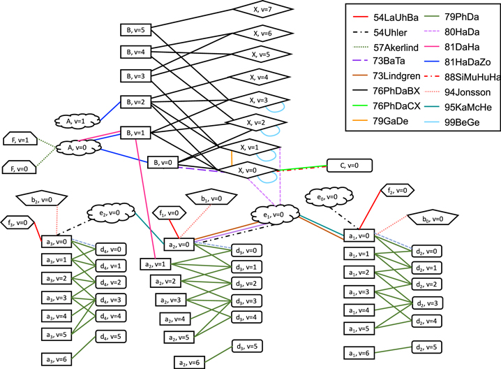
Figure 2. Depiction of connectivity of experimentally observed  bands.
Download figure:
Standard image High-resolution imageThere are three minor free-floating networks connecting the  (ν = 6) and
  (ν = 5) levels. These could be connected through observing additional vibrational transitions, but this is not essential for producing a good model of the
  electronic states.
3.2. Energy Levels
Table 4 shows an extract of the final empirical energy levels produced by Marvel for  in this work. This list of energy levels includes an estimate for the uncertainty in the provided energy of the quantum state, as well as identifying the number of transitions used to determine the energy level; on average, 5.3 transitions were used to find each energy level.
Table 4.
Extract from the 90Zr-16O.main.energies Output File for 
| State | v | J |

|
Unc. | No. |
|---|---|---|---|---|---|
| X1Sigma+ | 5 | 92 | 8286.730593 | 0.016290 | 3 |
| a3Delta_1 | 4 | 93 | 8289.132156 | 0.013142 | 3 |
| a3Delta_2 | 4 | 89 | 8295.024932 | 0.018098 | 3 |
| X1Sigma+ | 6 | 79 | 8296.993918 | 0.009580 | 6 |
| a3Delta_1 | 1 | 124 | 8312.622601 | 0.022336 | 7 |
| A1Delta | 0 | 76 | 8313.129649 | 0.004368 | 11 |
| a3Delta_2 | 5 | 76 | 8320.754165 | 0.013995 | 5 |
| a3Delta_2 | 3 | 101 | 8322.052377 | 0.013804 | 6 |
| a3Delta_2 | 1 | 121 | 8322.707720 | 0.012197 | 7 |
| X1Sigma+ | 4 | 104 | 8327.541550 | 0.020000 | 1 |
| A1Delta | 1 | 60 | 8336.081220 | 0.008485 | 2 |
| a3Delta_2 | 0 | 130 | 8336.647124 | 0.013307 | 6 |
Note. Energies and their uncertainties are given in cm−1. No indicates the number of transitions that contributed to the stated energy and uncertainty.
Download table as: ASCIITypeset image
Table 5 summarizes the 8088 empirical energy levels found in the main SN from the Marvel analysis for  . We see the minimum, average, and maximum uncertatinty provided for the empirical energies from the Marvel analysis. The minimum is usually very small, often less than 0.01 cm−1, while the maximum can exceed 0.1 cm−1; this is probably for higher J states. There is generally coverage to high rotational number J if the spin-vibronic level is known.
Table 5.
Summary of the 8088 Empirical Energy Levels for  Determined by Our Marvel analysis
| v | J Range | Uncertainties (cm−1) | |||
|---|---|---|---|---|---|
| Min | Av | Max | |||

|
0 | 0–131 | 1 × 10⁻⁷ | 0.0096 | 0.055 |
| 1 | 2–107 | 0.006 | 0.016 | 0.08 | |
| 2 | 2–115 | 0.0079 | 0.016 | 0.11 | |
| 3 | 2–105 | 0.008 | 0.014 | 0.052 | |
| 4 | 2–106 | 0.012 | 0.02 | 0.068 | |
| 5 | 2–107 | 0.0089 | 0.015 | 0.051 | |
| 6 | 2–107 | 0.0082 | 0.014 | 0.067 | |
| 7 | 3–66 | 0.012 | 0.016 | 0.042 | |

|
0 | 2–133 | 0.0031 | 0.0058 | 0.12 |
| 1 | 3–115 | 0.0045 | 0.012 | 0.14 | |
 e e |
0 | 1–133 | 0.0043 | 0.0075 | 0.065 |
| 1 | 1–116 | 0.0038 | 0.011 | 0.057 | |
| 2 | 1–117 | 0.0048 | 0.011 | 0.053 | |
| 3 | 1–108 | 0.0084 | 0.015 | 0.062 | |
| 4 | 1–116 | 0.0097 | 0.02 | 0.21 | |
| 5 | 2–67 | 0.01 | 0.018 | 0.045 | |
 f f |
0 | 1–133 | 0.0046 | 0.0089 | 0.15 |
| 1 | 1–118 | 0.0053 | 0.012 | 0.052 | |
| 2 | 2–115 | 0.0055 | 0.013 | 0.076 | |
| 3 | 2–106 | 0.012 | 0.02 | 0.08 | |
| 4 | 2–107 | 0.012 | 0.023 | 0.14 | |
| 5 | 3–66 | 0.014 | 0.019 | 0.042 | |

|
0 | 0–121 | 0.0041 | 0.02 | 0.21 |

|
0 | 17–102 | 0.057 | 0.063 | 0.14 |
| 1 | 35–93 | 0.057 | 0.064 | 0.1 | |
 1 1 |
0 | 2–150 | 0.0026 | 0.0072 | 0.063 |
| 1 | 2–150 | 0.007 | 0.014 | 0.12 | |
| 2 | 1–150 | 0.0074 | 0.013 | 0.084 | |
| 3 | 2–150 | 0.0072 | 0.013 | 0.059 | |
| 4 | 3–150 | 0.012 | 0.021 | 0.12 | |
| 5 | 2–106 | 0.0089 | 0.017 | 0.06 | |
 2 2 |
0 | 2–149 | 0.0023 | 0.0086 | 0.057 |
| 1 | 1–148 | 0.0052 | 0.014 | 0.08 | |
| 2 | 1–150 | 0.0072 | 0.017 | 0.2 | |
| 3 | 2–147 | 0.0075 | 0.018 | 0.17 | |
| 4 | 3–150 | 0.012 | 0.021 | 0.15 | |
| 5 | 2–136 | 0.0089 | 0.016 | 0.054 | |
 3 3 |
0 | 3–144 | 0.0024 | 0.013 | 0.2 |
| 1 | 3–144 | 0.0069 | 0.015 | 0.15 | |
| 2 | 3–145 | 0.0071 | 0.012 | 0.04 | |
| 3 | 3–135 | 0.0077 | 0.012 | 0.062 | |
| 4 | 3–105 | 0.012 | 0.017 | 0.043 | |
| 5 | 3–130 | 0.0082 | 0.014 | 0.055 | |
 0e 0e |
0 | 7–106 | 0.0035 | 0.0065 | 0.023 |
 0f 0f |
0 | 14–91 | 0.0042 | 0.0064 | 0.037 |
 1e 1e |
0 | 11–100 | 0.0035 | 0.0056 | 0.013 |
 1f 1f |
0 | 20–90 | 0.0036 | 0.0058 | 0.012 |
 2e 2e |
0 | 12–111 | 0.0035 | 0.0051 | 0.015 |
 2f 2f |
0 | 12–111 | 0.0035 | 0.0053 | 0.031 |
 2 2 |
0 | 2–150 | 0.0081 | 0.014 | 0.14 |
| 1 | 2–151 | 0.0071 | 0.013 | 0.22 | |
| 2 | 2–151 | 0.0075 | 0.013 | 0.056 | |
| 3 | 3–151 | 0.0069 | 0.011 | 0.035 | |
| 4 | 3–106 | 0.0086 | 0.014 | 0.041 | |
 3 3 |
0 | 3–148 | 0.01 | 0.018 | 0.12 |
| 1 | 2–151 | 0.0067 | 0.011 | 0.046 | |
| 2 | 2–147 | 0.0071 | 0.015 | 0.13 | |
| 3 | 2–150 | 0.0063 | 0.012 | 0.09 | |
| 4 | 3–136 | 0.0088 | 0.014 | 0.029 | |
 4 4 |
0 | 4–144 | 0.0081 | 0.016 | 0.11 |
| 1 | 4–145 | 0.0072 | 0.013 | 0.053 | |
| 2 | 4–145 | 0.0072 | 0.014 | 0.16 | |
| 3 | 4–145 | 0.0068 | 0.013 | 0.12 | |
| 4 | 4–131 | 0.0082 | 0.012 | 0.037 | |
 0e 0e |
0 | 15–59 | 0.058 | 0.07 | 0.1 |
 0f 0f |
0 | 27–59 | 0.058 | 0.064 | 0.15 |
 1e 1e |
0 | 3–73 | 0.0043 | 0.02 | 0.1 |
 1f 1f |
0 | 3–67 | 0.0044 | 0.016 | 0.13 |
 2 2 |
0 | 2–85 | 0.0043 | 0.034 | 0.1 |
 1 1 |
0 | 20–76 | 0.071 | 0.074 | 0.1 |
 2 2 |
0 | 20–79 | 0.071 | 0.075 | 0.1 |
 3 3 |
0 | 21–81 | 0.071 | 0.077 | 0.1 |
Our Marvel analysis shows that there is good rotationally resolved empirical understanding of a reasonable number of vibrational states of the  ,
,  ,
,  , and
, and  electronic states (sufficient for a good potential energy curve to be fitted). However, there is much less vibrational information (only one or two levels) for the
  ,
,  ,
,  ,
,  ,
,  , and
, and  states. This will cause significant problems when fitting potential energy curves for a full spectroscopic model and eventual line list for
  and its isotopologues, particularly for the
  ,
,  ,
,  , and
, and  states in which only one vibrational level is known. Note that line lists of all isotopologues can be easily produced using variational nuclear-motion techniques using data from only a single isotopologue with reasonably high accuracy; however, ab initio predictions of vibrational constants especially for higher lying electronic states of transition-metal-containing diatomics still have errors of up to 50 cm−1 (Tennyson et al. 2016).
Figure 3 shows the empirical energy levels for the main SN from Marvel against J for each spin-vibronic band. These are clearly quadratic and smooth, indicating there are no major problems with the Marvel network established for  .
.
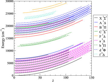
Figure 3.
 energy levels from the Marvel analysis.
Download figure:
Standard image High-resolution image3.3. Comparison with Plez et al. (2003)
Figure 4 shows the difference between the singlet Marvel energy levels for  and those from the Plez et al. (2003)
  line list. For the
  ,
,  , and
, and  states, the differences average around 0.05–0.15 cm−1, with somewhat higher deviations, up to 1 cm−1, for large J, especially in the
  state. The scatter here is probably largely a reflection of inaccuracies in the MARVEL energy levels, though perturbations not considered in the Plez line list might also contribute. The
  state, however, shows much more significant deviations; the v = 0 state is off by about 2 cm−1 up to J = 100, with much more significant deviations for larger J. The v = 1 state also shows substantial differences of up to 4 cm−1 that changes significantly with J.
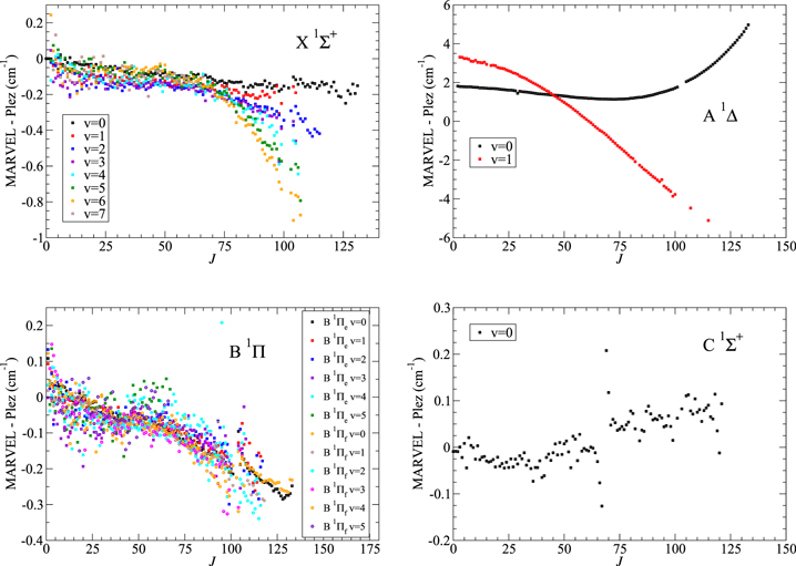
Figure 4. Difference between Marvel and Plez et al. (2003) energy levels for the singlet states.
Download figure:
Standard image High-resolution imageFigures 5–7 show the difference between the triplet Marvel energy levels for  and those from the Plez et al. (2003)
  line list. These deviations are much more significant than for the singlet states.
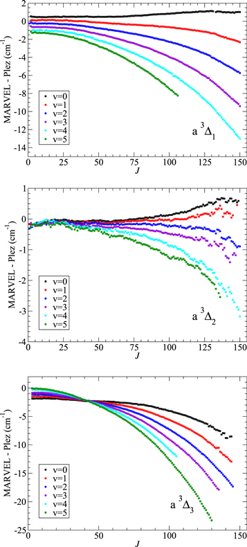
Figure 5. Difference between Marvel and Plez et al. (2003) energy levels for the  state.
Download figure:
Standard image High-resolution image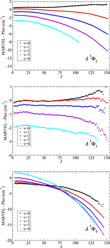
Figure 6. Difference between Marvel and Plez et al. (2003) energy levels for the  states.
Download figure:
Standard image High-resolution image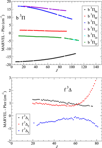
Figure 7. Difference between Marvel and Plez et al. (2003) energy levels for the  and
and  states.
Download figure:
Standard image High-resolution imageClear systematic errors can be seen throughout the  and
and  bands—since these are a major cause of opacity of
  in stellar conditions, improvements to these energy levels are highly desirable. Note, however, that since the errors in the
  n and
n and  n+1 parallel each other, the errors in transition frequencies in the Plez line list will be much smaller than the errors in energies that are plotted here.
The  state shows significant and systematic deviations in the Plez database compared to the Marvel data of up to 15 cm−1 for many vibronic levels. Our adoption of the Jonsson (1994) assignments in preference to the Phillips et al. (1979) assignments contributes to much larger Λ doubling in the Marvel data than was adopted in the Plez data. There are also clear systematic differences in the energies of the
  1 levels of more than 15 cm−1 in many regions. Smaller differences of up to 5 cm−1 were found in the
  2 levels that parallel the errors in the
  3 and
3 and  4 energies, indicating that the errors associated with the transition frequencies in this band in the Plez line list will be much smaller.
The  data show that Plez’s triplet splitting is in error by about 1 cm−1, with some larger errors at high J.
3.4. Band Constants
Band constants were obtained by a quadratic fit of the energies of the lines against rotational quantum number J for each band.
Table 6 shows the rotational band constants, Tv, Bv, and Dv for each singlet vibronic bands. The centrifugal term, Dv, is reasonably constant within a given electronic state, while the rotational constant, Bv, decreases as expected as the bond length increases in higher vibrational states.
Table 6. Spectroscopic Band Constants, in cm−1, for the Singlet Vibronic Bands, Assuming No Perturbations
| State | v | Tv | Bv | 107 Dv |
|---|---|---|---|---|

|
0 | −0.028 | 0.4226 | 3.18 |
| 1 | 969.509 | 0.42065 | 3.19 | |
| 2 | 1932.154 | 0.41868 | 3.18 | |
| 3 | 2887.873 | 0.41674 | 3.22 | |
| 4 | 3836.760 | 0.41475 | 3.22 | |
| 5 | 4778.739 | 0.41275 | 3.21 | |
| 6 | 5713.739 | 0.41077 | 3.23 | |

|
0 | 5887.160 | 0.41646 | 3.26 |
| 1 | 6823.105 | 0.41457 | 3.26 | |

|
0 | 15383.385 | 0.40151 | 3.51 |
| 1 | 16236.949 | 0.39959 | 3.50 | |
| 2 | 17084.607 | 0.39765 | 3.51 | |
| 3 | 17926.299 | 0.39570 | 3.51 | |
| 4 | 18762.010 | 0.39375 | 3.52 | |
| 5 | 19591.668 | 0.39175 | 3.40 | |

|
0 | 17050.378 | 0.40480 | 3.44 |

|
0 | 25159.631 | 0.39736 | 3.57 |
| 1 | 25994.872 | 0.39540 | 3.66 |
Download table as: ASCIITypeset image
Table 7 shows the fitted rotational band constants for each spin-vibronic band in the triplet manifold for  from this Marvel analysis.
Table 7. Spectroscopic Constants, in cm−1, for the Triplet Spin-vibronic Bands, Assuming No Perturbations
| Σ = −1 | Σ = 0 | Σ = 1 | ||||||||
|---|---|---|---|---|---|---|---|---|---|---|
| v | Tv | Bv | Dv(107) | Tv | Bv | Dv(107) | Tv | Bv | Dv(107) Δ(SO) | |
 1 1 |
 2 2 |
 3 3 |
||||||||
| 0 | 1080.363 | 0.41333 | 3.18 | 1367.750 | 0.41476 | 3.26 | 1703.505 | 0.41565 | 3.43 | |
| 1 | 2011.656 | 0.41144 | 3.19 | 2299.369 | 0.41285 | 3.26 | 2635.505 | 0.41374 | 3.44 | |
| 2 | 2936.474 | 0.40955 | 3.20 | 3224.476 | 0.41096 | 3.29 | 3561.029 | 0.41181 | 3.45 | |
| 3 | 3854.766 | 0.40765 | 3.21 | 4143.140 | 0.40903 | 3.28 | 4480.011 | 0.40989 | 3.45 | |
| 4 | 4766.602 | 0.40574 | 3.22 | 5055.317 | 0.40712 | 3.31 | 5392.650 | 0.40791 | 3.43 | |
| 5 | 5672.050 | 0.40378 | 3.19 | 5960.981 | 0.40516 | 3.28 | 6298.588 | 0.40602 | 3.48 | |
 0 0 |
 1 1 |
 2 2 |
||||||||
| 0 | e | 11765.173 | 0.40801 | 3.36 | 12069.846 | 0.40862 | 3.42 | 12427.697 | 0.40934 | 3.62 |
| f | 11783.845 | 0.40754 | 3.29 | 12069.859 | 0.40915 | 3.45 | 12427.705 | 0.40933 | 3.60 | |
 2 2 |
 3 3 |
 4 4 |
||||||||
| 0 | 16507.187 | 0.40312 | 3.57 | 17109.068 | 0.40368 | 3.60 | 17737.310 | 0.40430 | 3.77 | |
| 1 | 17357.358 | 0.40103 | 3.58 | 17958.303 | 0.40160 | 3.62 | 18588.627 | 0.40222 | 3.77 | |
| 2 | 18200.953 | 0.39894 | 3.59 | 18801.000 | 0.39949 | 3.63 | 19433.859 | 0.40015 | 3.78 | |
| 3 | 19038.014 | 0.39683 | 3.60 | 19637.131 | 0.39738 | 3.65 | 20273.306 | 0.39807 | 3.77 | |
| 4 | 19868.503 | 0.39469 | 3.58 | 20466.627 | 0.39524 | 3.62 | 21106.945 | 0.39602 | 3.77 | |
 0 0 |
 1 1 |
 2 2 |
||||||||
| 0 | e | 19074.117 | 0.39551 | 0.85 | 19113.069 | 0.40387 | 5.73 | 19169.508 | 0.40619 | 5.02 |
| f | 19078.935 | 0.39449 | 0.04 | 19112.826 | 0.40266 | 4.79 | ||||
 1 1 |
 2 2 |
 3 3 |
||||||||
| 0 | 22616.840 | 0.38945 | 3.43 | 22916.797 | 0.39207 | 0.67 | 23335.153 | 0.39572 | 3.01 | |
Download table as: ASCIITypeset image
A compilation of band constants is given by Kaledin et al. (1995); we find significant differences of 2 cm−1 in the T0 for  2,
2,  3, and
  3. We prefer our value, however, as the
  —
— transitions form part of our input data, whereas it is unclear how the Kaledin et al. (1995) was compiled. Otherwise, the T0 values agree within 0.1 cm−1.
3.5. Bandheads
Tables 8–12 show bandheads predicted by the Marvel energy levels, compared with available, low-resolution bandhead observations (note that the high-resolution bandhead observations are included in the Marvel input data set). For the singlet states, there is actually only a small number of data points in the  –
– band that allow for direct comparison of Marvel predictions against low-resolution bandhead studies. There are no assigned low-resolution data readily available for the
  –
– band, and the low-resolution bandhead data for
  –
– does not overlap with our Marvel predictions. For the triplets, there is good low-resolution bandhead data for the
  –
– ,
,  –
– , and
, and  –
– bands against which the Marvel results can be compared; in these cases, there is good agreement for all bands, generally better than 0.5 cm−1 (though up to 1.5 cm−1).
Table 8.
R-branch Bandheads in cm−1 From the  State for
  ; J Gives the Approximate J Value Corresponding to the Rotational Transitions at the Bandhead
| v′–v″ | J | MARVEL | Low-res obs. | |
|---|---|---|---|---|
 – –
|
0–0 | 18 | 15391.40 | ⋯ |
| 0–1 | 20 | 14422.64 | ⋯ | |
| 0–2 | 22 | 13460.94 | ⋯ | |
| 0–3a | 25 | 12506.31 | ⋯ | |
| 0–4a | 29 | 11559.08 | ⋯ | |
| 0–5a | 34 | 10619.12 | ⋯ | |
| 0–6a | 41 | 9687.00 | ⋯ | |
| 0–7a | 53 | 8763.33 | ⋯ | |
| 1–0 | 18 | 16244.28 | ⋯ | |
| 1–1a | 18 | 15275.39 | ⋯ | |
| 1–2 | 21 | 14313.52 | ⋯ | |
| 1–3 | 22 | 13358.69 | ⋯ | |
| 1–4a | 24 | 12410.99 | ⋯ | |
| 1–5a | 30 | 11470.63 | ⋯ | |
| 1–6a | 36 | 10537.59 | ⋯ | |
| 1–7a | 43 | 9612.56 | ⋯ | |
| 2–0 | 15 | 17091.34 | ⋯ | |
| 2–1 | 17 | 16122.32 | ⋯ | |
| 2–2a | 18 | 15160.33 | ⋯ | |
| 2–3 | 21 | 14205.29 | ⋯ | |
| 2–4 | 22 | 13257.41 | ⋯ | |
| 2–5a | 26 | 12316.62 | ⋯ | |
| 2–6a | 30 | 11383.20 | ⋯ | |
| 2–7a | 25 | 10457.20 | ⋯ | |
| 3–0a | 15 | 17932.50 | ⋯ | |
| 3–1 | 14 | 16963.46 | ⋯ | |
| 3–2a | 17 | 16001.36 | ⋯ | |
| 3–3a | 17 | 15046.20 | ⋯ | |
| 3–4a | 21 | 14098.05 | ⋯ | |
| 3–5 | 22 | 13157.07 | ⋯ | |
| 3–6 | 27 | 12223.20 | ⋯ | |
| 3–7a | 31 | 11296.67 | ⋯ | |
| 4–0a | 14 | 18767.79 | ⋯ | |
| 4–1a | 14 | 17798.67 | ⋯ | |
| 4–2 | 16 | 16836.45 | ⋯ | |
| 4–3a | 17 | 15881.27 | ⋯ | |
| 4–4a | 17 | 14933.00 | ⋯ | |
| 4–5 | 20 | 13991.83 | ⋯ | |
| 4–6 | 21 | 13057.77 | ⋯ | |
| 4–7a | 26 | 12130.78 | ⋯ | |
| 5–0a | 11 | 19597.03 | ⋯ | |
| 5–1a | 13 | 18627.83 | ⋯ | |
| 5–2a | 13 | 17665.63 | ⋯ | |
| 5–3 | 14 | 16710.22 | ⋯ | |
| 5–4a | 17 | 15761.90 | ⋯ | |
| 5–5a | 20 | 14820.57 | ⋯ | |
| 5–6a | 20 | 13886.36 | ⋯ | |
| 5–7 | 21 | 12959.14 | ⋯ | |
 – –
|
0–0 | 22 | 17059.99 | ⋯ |
| 0–1a | 25 | 16091.58 | ⋯ | |
| 0–2a | 28 | 15130.40 | ⋯ | |
| 0–3a | 33 | 14176.55 | ⋯ | |
| 0–4a | 41 | 13230.35 | ⋯ | |
| 0–5a | 49 | 12292.37 | ⋯ | |
| 0–6a | 82 | 11365.35 | ⋯ | |
| 1–0 | ⋯ | ⋯ | 17933b | |
| 2–0 | ⋯ | ⋯ | 18799b | |
| 3–0 | ⋯ | ⋯ | 19664b |
Notes.
aBands unobserved in rotationally resolved spectra that have been predicted by Marvel. bBalfour & Chowdhury (2010; converted from wavelength assuming vacuum).Download table as: ASCIITypeset image
Table 9.
Other Singlet R-branch Bandheads in cm−1 for  ; J Gives the Approximate J Value Corresponding to the Rotational Transitions at the Bandhead
| v′–v″ | J | MARVEL | Low-res obs. | |
|---|---|---|---|---|
 – –
|
0–0 | 17 | 25166.23 | ⋯ |
| 0–1 | 18 | 24197.07 | ⋯ | |
| 0–2 | 17 | 23235.27 | ⋯ | |
| 0–3 | 22 | 22280.33 | ⋯ | |
| 0–4 | 22 | 21332.47 | ⋯ | |
| 0–5 | 25 | 20391.58 | ⋯ | |
| 0–6 | 30 | 19458.10 | ⋯ | |
| 0–7 | 35 | 18531.99 | ⋯ | |
 – –
|
2–0 | 101 | 1975.73 | ⋯ |
| 3–0 | 68 | 2917.35 | ⋯ | |
| 3–1 | 99 | 1961.43 | ⋯ | |
| 4–0 | 51 | 3858.92 | ⋯ | |
| 4–1 | 65 | 2896.33 | ⋯ | |
| 4–2 | 99 | 1948.15 | ⋯ | |
| 5–0 | 42 | 4796.37 | ⋯ | |
| 5–1 | 51 | 3831.03 | ⋯ | |
| 5–2 | 67 | 2875.26 | ⋯ | |
| 5–3 | 98 | 1932.88 | ⋯ | |
| 6–0 | 33 | 5728.41 | ⋯ | |
| 6–1 | 41 | 4761.69 | ⋯ | |
| 6–2 | 49 | 3803.14 | ⋯ | |
| 6–3 | 67 | 2854.22 | ⋯ | |
| 6–4 | 98 | 1918.42 | ⋯ | |
| 7–0 | 28 | 6654.41 | ⋯ | |
| 7–1 | 33 | 5686.80 | ⋯ | |
| 7–2 | 40 | 4726.86 | ⋯ | |
| 7–3 | 50 | 3775.20 | ⋯ | |
 – –
|
0–0 | 26 | 9507.28 | 9507.45a |
| 0–1 | 30 | 8572.87 | ⋯ | |
| 1–0 | 23 | 10359.55 | 10359.62a | |
| 1–1b | 25 | 9424.77 | 9424.93a | |
| 2–0 | 21 | 11206.15 | ⋯ | |
| 2–1 | 22 | 10271.14 | 10271.26a | |
| 3–0b | 17 | 12047.00 | ⋯ | |
| 3–1 | 21 | 11111.79 | ⋯ | |
| 4–0b | 17 | 12882.08 | ⋯ | |
| 4–1b | 17 | 11946.74 | ⋯ | |
| 5–0b | 15 | 13711.04 | ⋯ | |
| 5–1b | 17 | 12775.64 | ⋯ | |
 – –
|
0–0b | 33 | 11177.59 | ⋯ |
| 0–1b | 41 | 10244.31 | ⋯ | |
 – –
|
0–0 | 22 | 19281.19 | ⋯ |
| 0–1 | 22 | 18346.21 | ⋯ |
Notes.
aBalfour & Chowdhury (2010; converted from wavelength assuming vacuum). bBands unobserved in rotationally resolved spectra that have been predicted by Marvel.Download table as: ASCIITypeset image
Table 10.
Other Singlet R-branch Bandheads in cm−1 for  ; J Gives the Approximate J Value Corresponding to the Rotational Transitions at the Bandhead
| v′–v″ | J | MARVEL | |
|---|---|---|---|
 – –
|
0–0 | 91 | 9814.07 |
| 1–0 | 61 | 10637.34 | |
| 1–1 | 90 | 9794.47 | |
 – –
|
2–0 | 53 | 56.81 |
| 3–0 | 41 | 893.65 | |
| 4–0 | 34 | 1726.14 | |
| 5–0 | 28 | 2553.57 | |
 – –
|
0–0 | 50 | 8130.59 |
| 1–0 | 40 | 8961.46 |
Download table as: ASCIITypeset image
Table 11.
Triplet  –
– and
and  –
– R-branch Bandheads in cm−1 for
  ; J Gives the Approximate J Value Corresponding to the Rotational Transitions at the Bandhead
| v′–v″ | J | MARVEL | Low-res obs. | |
|---|---|---|---|---|
 1– 1–
|
0–0 | ⋯ | ⋯ | 19124a |
| 1–0 | ⋯ | ⋯ | 19963a | |
| 2–0 | ⋯ | ⋯ | 20784a | |
 0e– 0e– 1 1 |
0–0 | 72 | 10715.52 | 10715.26b |
| 0–1c | 101 | 9798.16 | ⋯ | |
| 1–1 | ⋯ | ⋯ | 10634.15b | |
 0f– 0f– 1 1 |
0–0 | 67 | 10731.97 | 10731.92a |
 1e– 1e– 2 2 |
0–0 | 63 | 10729.02 | 10728.98a |
| 0–1c | 89 | 9808.11 | ⋯ | |
 1f– 1f– 2 2 |
0–0 | 67 | 10731.44 | 10731.29a |
| 1–1 | ⋯ | ⋯ | 10649.82b | |
 2– 2– 3 3 |
0–0 | 62 | 10750.52 | ⋯ |
| 0–1 | 81 | 9828.65 | ⋯ | |
 1e– 1e– 2 2 |
0–0 | 34 | 17760.35 | ⋯ |
| 0–1c | 40 | 16831.39 | 16833.0d | |
| 0–2c | 49 | 15909.87 | 15909.2d | |
| 0–3c | 58 | 14996.56 | 14994.3d | |
 1f– 1f– 2 2 |
0–0 | 32 | 17758.67 | ⋯ |
| 0–1c | 38 | 16829.39 | 16833.0d | |
| 0–2c | 44 | 15907.41 | 15909.2d | |
| 0–3c | 55 | 14993.55 | 14994.5d | |
 1– 1– 2 2 |
1–1 | ⋯ | ⋯ | 17669.2d |
| 1–2 | ⋯ | ⋯ | 16747.2d | |
| 1–3 | ⋯ | ⋯ | 15556.1d | |
| 1–4 | ⋯ | ⋯ | 14923.9d | |
Notes.
aMeasured (Davis & Hammer 1981) reassigned here. bBalfour & Chowdhury (2010; converted from wavelength assuming vacuum). cBands unobserved in rotationally resolved spectra that have been predicted by Marvel. dStepanov et al. (1988).Download table as: ASCIITypeset image
Table 12.
d3Φ–a3Δ R-branch Bandheads in cm−1 for  from the Main Spectroscopic Networks; J Gives the Location of the Bandhead in Our Data
| v′–v″ | J | MARVEL | Low-res obs. | J | MARVEL | Low-res obs. | J | MARVEL | Low-res obs. |
|---|---|---|---|---|---|---|---|---|---|
 2– 2– 1 1 |
 3– 3– 2 2 |
 4– 4– 3 3 |
|||||||
| 0–0 | 39 | 15443 | 15443.0a | 34 | 15756.3 | 15756.3a | 36 | 16048.46 | 16048.6a |
| 0–1 | 48 | 14515.12 | 43 | 14827.63 | 42 | 15119.3 | 15119.2a | ||
| 0–2b | 57 | 13595.58 | 52 | 13906.89 | 51 | 14198.01 | |||
| 0–3b | 78 | 12686.13 | 67 | 12995.36 | 68 | 13285.67 | |||
| 0–4b | 108 | 11790.97 | 96 | 12096.25 | 90 | 12385.29 | |||
| 1–0 | 32 | 16290.36 | 16290.4a | 30 | 16603.14 | 16603.4a | 30 | 16897.5 | 16897.4a |
| 1–1 | 37 | 15361.4 | 15361.4a | 34 | 15673.57 | 15673.5a | 35 | 15967.47 | 15967.9a |
| 1–2 | 44 | 14439.86 | 40 | 14751.22 | 40 | 15044.66 | 15044.0a | ||
| 1–3b | 57 | 12526.53 | 51 | 13836.77 | 51 | 14129.7 | |||
| 1–4b | 76 | 12623.07 | 68 | 12931.37 | 67 | 13223.55 | |||
| 1–5b | 104 | 11733.3 | 94 | 12047.9 | 87 | 12329 | |||
| 2–0b | 27 | 17132.02 | 17132.9a | 26 | 17444.03 | 17444.7a | 25 | 17741.09 | |
| 2–1 | 16202.5a | 28 | 16513.89 | 16514.0a | 29 | 16810.47 | 16810.6a | ||
| 2–2 | 36 | 15279.76 | 15279.8a | 34 | 15590.72 | 15590.8a | 33 | 15886.85 | 15886.9a |
| 2–3b | 45 | 14364.58 | 40 | 14674.79 | 39 | 14970.55 | 14970.7a | ||
| 2–4b | 54 | 13457.5 | 51 | 13766.6 | 51 | 14061.86 | |||
| 2–5b | 74 | 12560.01 | 64 | 12867.46 | 64 | 13161.97 | |||
| 3–0b | 23 | 17967.59 | 22 | 18278.87 | 23 | 18579.17 | |||
| 3–1b | 26 | 17037.47 | 17036.2a | 24 | 17348.38 | 17347.7a | 25 | 17648.31 | 17646.7a |
| 3–2 | 29 | 16114.24 | 16114.2a | 27 | 16424.59 | 16424.7a | 29 | 16724.12 | 16724.3a |
| 3–3 | 35 | 15198.07 | 15298.4a | 34 | 15507.83 | 15508.2a | 33 | 15807.01 | 15807.6a |
| 3–4 | 41 | 14289.18 | 39 | 14597.25 | 40 | 14897.02 | 14897.2a | ||
| 3–5 | 54 | 13388.34 | 47 | 13696.37 | 51 | 13994.73 | |||
| 4–0b | 21 | 18796.88 | 19 | 19107.25 | 19 | 19411.79 | |||
| 4–1b | 24 | 17866.54 | 21 | 18176.52 | 22 | 18480.69 | |||
| 4–2b | 25 | 16942.87 | 16942.5a | 24 | 17252.48 | 17253.3a | 24 | 17556.27 | 17555.6a |
| 4–3 | 29 | 16026.05 | 16025.0a | 28 | 16335.14 | 16335.6a | 27 | 16638.61 | 16638.6a |
| 4–4b | 36 | 15116.29 | 15115.2a | 34 | 15424.86 | 15425.2a | 31 | 15727.82 | 15728.3a |
| 4–5 | 43 | 14213.74 | 39 | 14521.64 | 39 | 14824.26 | |||
| 5–3b | 16847.4a | 17463.2a | |||||||
| 5–4b | 15936.9a | 16554.2a | |||||||
| 5–5b | 15034.8a | 15342.6a | 15648.8a | ||||||
Notes.
aStepanov et al. (1988). bBands unobserved in rotationally resolved spectra that have been predicted by Marvel.Download table as: ASCIITypeset image
The Marvel results provide predictions for 48 vibronic bands previously unmeasured in low or high-resolution spectra. In contrast, there are at least 68 additional low-resolution bandheads whose positions cannot be predicted by our Marvel data due to lack of information on, usually, the excited state. The most significant missed opportunity for rotational resolved data is in the 48 nonsatellite, i.e., ΔΣ = 0,  –
– bandheads for v = 0 to v = 6 observed in low-resolution by Stepanov et al. (1988); note that these data are not reported in this paper. Much lower resolution bandheads are identified by Balfour & Chowdhury (2010) for the
  –
– band involving excited vibrational levels of the
  state; this too warrants further investigation to allow characterization of the
  state.
There have also been some bandheads discussed in previous  spectroscopic studies that our data unfortunately cannot help assign. Specifically, we do not find any recommended assignment of the double bandhead at 12,082.65 cm−1 (R head) and 12,069.9 cm−1 (Q head) observed by Davis & Hammer (1981).
3.6. Equilibrium Constants: Updated Recommendations
Table 13 shows equilibrium term energy, vibrational, and rotational constants for the  ,
,  ,
,  ,
,  ,
,  1,
1,  2,
2,  3,
3,  2,
2,  3, and
  4 electronic states based entirely on Marvel energy levels. These equilibrium constants are obtained by fitting to the relevant band constants, with obvious outliers removed for averaging of Dv's to obtain D. Note that we have chosen to provide constants for the various subcomponents of the triplet levels individually rather than use additional constants to unify their treatment.
Table 13. Equilibrium Vibrational Constants, in cm−1, Based Solely on Marvel Energy Levels
| State | Te | ωe | ωeχe | Be | α(103) | D(107) |
|---|---|---|---|---|---|---|

|
0 | 976.44 | 3.45 | 0.42361 | 1.97 | 3.19 |

|
5906.58 | 935.95 | ⋯ | 0.41741 | 1.89 | 3.26 |

|
15441.70 | 859.59 | 2.99 | 0.40246 | 1.90 | 3.50 |

|
25229.40 | 835.24 | ⋯ | 0.39834 | 1.96 | 3.60 |
 1 1 |
1099.70 | 937.74 | 3.23 | 0.41430 | 1.91 | 3.19 |
 2 2 |
1386.90 | 938.09 | 3.24 | 0.41573 | 1.92 | 3.26 |
 3 3 |
1722.45 | 938.51 | 3.25 | 0.41663 | 1.93 | 3.43 |
 2 2 |
16567.04 | 856.72 | 3.27 | 0.40419 | 2.11 | 3.57 |
 3 3 |
17169.35 | 855.84 | 3.29 | 0.40475 | 2.11 | 3.61 |
 4 4 |
17796.92 | 857.09 | 2.94 | 0.40533 | 2.07 | 3.77 |
Download table as: ASCIITypeset image
Based on a comprehensive collation and critical analysis of all available information (to our knowledge) of spectroscopic constants, we can go beyond this Marvel analysis to provide recommendations for all equilibrium constants for the electronic states of  ; these are shown in Tables 14 and 15. Some of these constants come solely from the Marvel analysis in this paper, but some use other sources of data, particularly for vibrational anharmonicities where lower resolution bandhead data can provide additional information. Note that because we do not consider higher order corrections to D or α within these constants, we use D and α rather than De and αe.
Table 14.
Recommended Updated Equilibrium Constants in cm−1 for Triplet States of  , with Bond Lengths in Å
| State | Te | ωe | ωexe | Be | α(10−3) | D(10−7) | re |
|---|---|---|---|---|---|---|---|

|
0.0 | 976.44(2) | 3.44(2) | 0.4236(1) | 1.97(2) | 3.2(1) | 1.712(2) |

|
5906.6(2) | 942.3(2) | 3.1(1) | 0.4174(1) | 1.89(1) | 3.3(1) | 1.725(2) |

|
15441.7(2) | 859.6(2) | 3.0(1) | 0.4025(1) | 1.90(1) | 3.5(2) | 1.756(2) |

|
17101(1) | 876(1) | 3.0(2) | 0.4056(1) | 1.65(1) | 3.4(1) | 1.750(3) |

|
25227(1) | 841(1) | 2.9(2) | 0.3983(3) | 2.0(1) | 3.6(2) | 1.765(2) |
Note. The value in the parenthesis is the uncertainty in the last figure. Justifications for each electronic state are provided in the text.
Download table as: ASCIITypeset image
Table 15.
Recommended Updated Equilibrium Constants in cm−1 for Singlet States of  , with Bond Lengths in Å
| State |

|

|

|
ωe | ωexe | Be | αe(10−3) | D(10−7) | re |
|---|---|---|---|---|---|---|---|---|---|

|
1099.7(7) | 1386.9(5) | 1722.4(9) | 938.1(4) | 3.24(1) | 0.415(1) | 1.93(4) | 3.3(1) | 1.729(2) |

|
11807(1), 11826(1) | 12112(1) | 12469(4) | 890(1) | 3.2(3) | [0.409](1) | ⋯ | 3.5(3) | 1.741(2) |

|
16567(1) | 17169(1) | 17796(1) | 855(1) | 3.0(2) | 0.404(1) | 2.10(3) | 3.6(1) | 1.751(2) |

|
19138(1), 19142(1) | 19177(1) | 19233(1) | 846(1) | 3.1(2) | [0.401](1) | ⋯ | 5(2) | 1.756(2) |

|
22692(1) | 22993(1) | 23411(1) | 821(1) | 3.3(2) | [0.392](2) | ⋯ | 3.1(6) | 1.776(2) |
Note. Square brackets indicate the data is only from v = 0. The value in the parenthesis is the uncertainty in the last figure. Justifications for each electronic state are provided in the text.
Download table as: ASCIITypeset image
Note that these constants will provide less accurate information on particular energy levels than the raw Marvel energy levels, but have the advantage of being a smaller, more easily parsed set of numbers. Thus, we have chosen to average across different parity and spin states in most cases, though we retain the term values (Te) for individual spin components of the triplet states.
The justification for each of the constants in Tables 14 and 15 are as follows:
- 1.
- 2. Rotational constants are from Marvel analysis, while the equilibrium vibrational constants are taken from Hammer & Davis (1981; only values available). Consistency with Marvel Tv's has been checked. Note that Hammer & Davis (1981) have rotational band constants and equilibrium vibrational constants involving v > 1, but do not provide transition data involving this level; thus it is excluded from the Marvel compilation.
- 3.
- 4. Vibrational constants are taken from Murty (1980a), which is based on mostly Phillips & Davis (1976a) data. Be and αe were also from Murty (1980a) with uncertainties chosen to ensure consistency with other available data, including Marvel's B0 values. The centrifugal distortion term D is by necessity a v = 0 constant rather than an equilibrium value and thus is taken from Marvel with uncertainties determined by comparison to Simard et al. (1988b) and Phillips & Davis (1976a). Recommended equilibrium term energy Te is based on T0 from Marvel data and the adopted vibrational constants.
- 5. Based on values for other states, ωexe = 2.9(2) seems reasonable; we use this value and other Marvel Te data to obtain equilibrium term energy and vibrational constants. Rotational constants are taken from Marvel values.
- 6. Marvel data are used, averaged over the various spin states for vibrational and rotational equilibrium constants. Uncertainties are estimated largely based on the difference between constants of the three different spin components.
- 7. Rotational resolution and thus Marvel data are only available for the v = 0 levels; thus rotational v = 0 band constants are provided rather than rotational equilibrium constants, while vibrational constants are taken from Jonsson (1994). Uncertainties in rotational band constants were estimated by comparing values from the different spin components. Uncertainties in vibrational constants were taken as 1 cm−1 based on typical differences between vibrational constants for the three spin components for ZrO triplet states.
- 8. Constants are taken from Marvel data, with uncertainties estimated based on the difference between the constants from the three different spin components.
- 9. There are no rotationally resolved v > 0 data, so we recommend vibrational equilibrium constants from Stepanov et al. (1988) based on bandhead data. Rotational data are band constants from Marvel v = 0 levels. The equilibrium term energies, Te, are calculated from the adopted equilibrium constants and Marvel T0 values. Note that there is significant enough Λ-doubling in the 0 levels to justify a separate report of different Te values, whereas this effect is negligible at the likely accuracy of these constants for the 1 and 2 levels.
- 10. The Huber & Herzberg (1979; HH) data has been retained for the vibrational equilibrium constants since there have been no subsequent experiments involving this state and no rotationally resolved spectral data for levels above v = 0 that could be utilized in the Marvel analysis. For the rotational constants, Marvel data has been used, with uncertainties determined by the difference between the Marvel and HH values (these are quite close) and the spread of values among different spin components. Note that the fitted D0 constants for the 2 band seem to be the result of perturbations; thus it has been largely ignored in the averaging. The equilibrium term energies, Te, are based on Marvel T0 and HH vibrational constants.


The spectroscopic constants given in Tables 14 and 15 can be considered to provide a much needed update to the  entry in the still very commonly used Huber & Herzberg (1979; HH) compilation of diatomic constants. Note that the HH data was collated up to 1975 August, i.e., before a substantial number of the experiments, particularly the infrared spectra of Gallaher & Devore (1979) and many spectra recorded by Davis and coauthors during the 1970s and 1980s. There have been significant relabeling of the electronic states over the years; we adopt the convention shown in Figure 1, with some other labels, including the HH labels, shown in brackets. Our comments here use the updated notation.
A key difference between HH and our recommendations is in the harmonic vibrational frequency of the  ground state: 969.7 cm−1 (HH) versus 976.38 cm−1 (Marvel and our recommended value). This difference arises because the HH value is taken from a neon matrix spectrum (rather than a gas phase spectrum), which is known to cause shifts in vibrational frequencies.
All triplet states and the  state harmonic vibrational frequencies from HH were obtained from bandhead data; we update the
  ,
,  , and
, and  values with rotationally resolved data. For all states except the
  ,
,  , and
, and  states, the harmonic vibrational constants from Huber & Herzberg (1979) are within 2–4 cm−1 of our results. Our
  and
and  vibrational constants are based on low-resolution results from Balfour & Chowdhury (2010) and would need to be further verified; however, they should be more reliable than those of HH.
HH does not contain any information on the observed  or
or  states or the theoretically predicted
  ,
,  , and
, and  states. HH did not have access to the triplet-singlet separation, instead leaving an “x” off-set between the singlet and triplet manifolds. This was measured by Hammer & Davis (1980) as 1100 cm−1. The Te for the
  ,
,  ,
,  , and
, and  states are within 2 cm−1 (Marvel versus HH). HH does not have absolute or relative Te for the
  state.
Therefore, the key updates to HH from our results are:
- 1.updated vibrational constants for the state;
- 2.inclusion of the, state;
- 3.absolute Te of the state; and
- 4.absolute Te for triplet states.


These updates are important to note given the widespread use of the HH constants for a wide variety of applications from benchmarking quantum chemistry (Langhoff & Bauschlicher 1990) to calculating partition functions and equilibrium constants for astrophysical atmosphere models (Sauval & Tatum 1984; Barklem & Collet 2016).
We note that we are not the first, of course, to update some of the HH constants (e.g., see Afaf 1987; Davis & Hammer 1988; Langhoff & Bauschlicher 1990); this update is, however, comprehensive and based on a complete self-consistent data set containing all available assigned rovibronic spectra of ZrO.
3.7. Partition Function
Table 16 shows the partition function for  at a range of temperatures. These are predicted in two ways: using just Marvel energy levels and using Marvel energy levels and the contributions from rovibronic states not in the Marvel collation up to v = 15 and J = 300 for the
  ,
,  ,
,  ,
,  ,
,  ,
,  ,
,  , and
, and  states. We also compare against results from Shankar & Littleton (1983), Sauval & Tatum (1984), and Barklem & Collet (2016). From these results, it is obviously essential at high temperatures to incorporate the effect of energy levels not considered in the Marvel collation of energy levels (i.e., extrapolate beyond available experimental data). When this is done, the four results are all consistent within 2.6% at 5000 K. The key differences between the methodology for these four results are (1) explicit summation of energy levels as done in this paper versus high temperature summation expression used by previous authors, (2) the number of electronic states considered, and (3) minor changes in the spectroscopic constants used. We have checked the convergence of the explicit sum of our partition function in terms of the values of v and J and the number of electronic states included and found it to be consistent within four significant figures, the accuracy of our input constants, at 5000 K. Therefore, we recommend using our Marvel + constants partition function values, as tabulated at 1 K intervals in the supporting information.
Table 16.
Partition Function for  as a Function of Temperature (T) Estimated Based on the New Marvel Data and Reasonable Extrapolations
| T/K | 0 | 1 | 10 | 100 | 300 | 500 | 800 | 1000 | 1500 | 2000 | 3000 | 5000 |
|---|---|---|---|---|---|---|---|---|---|---|---|---|
| MARVEL only | 1. | 2.02446 | 16.8071 | 164.881 | 506.325 | 1006.32 | 2508.94 | 4185.61 | 11082.6 | 21884.9 | 53261.5 | 136797. |
| MARVEL + constants | 1. | 2.02446 | 16.8071 | 164.881 | 506.398 | 1006.87 | 2510.93 | 4190.11 | 11157.3 | 22472.4 | 59845.3 | 209393. |
| Shankar & Littleton (1983) | ⋯ | ⋯ | ⋯ | ⋯ | ⋯ | ⋯ | ⋯ | 4184.00 | 11140.0 | 22450.0 | 59790.0 | 211700. |
| Sauval & Tatum (1984) | ⋯ | ⋯ | ⋯ | ⋯ | ⋯ | ⋯ | ⋯ | 4167.99 | 11333.9 | 22729.5 | 60236.7 | 208621. |
| Barklem & Collet (2016) | 1 | 2.02843 | 16.8283 | 165.280 | 507.801 | 1010.06 | ⋯ | 4209.23 | 11234.5 | 22679.4 | 60617.8 | 214087. |
Download table as: ASCIITypeset image
3.8. Recommended Experiments
It would be desirable to obtain rovibronically resolved spectra involving the higher vibrational states for the  ,
,  , and
, and  states (for which only v = 0 is measured) and the
  and
and  states (for which only v = 0 and v = 1 are measured). This is critical for a high quality spectroscopic study of the molecule; currently, line lists would need to rely on lower quality nonrotationally resolved data to understand the vibrational structure. We can use the theoretical investigation of
  by Langhoff & Bauschlicher (1990) to guide our predictions for the ease of detecting these new transitions. The
  state is only reasonably accessible via relaxation or stimulated emission from the
  state or through high temperature initial population; several vibrational levels of
  can be populated through observed, high intensity, transitions, however. The
  state is directly accessibly from the ground
  state; the spectral region for the
  –
– 1–0 transition is estimated at around 18,000 cm−1 and should have reasonable Franck–Condon intensity. Other vibronic bands of
  –
– will probably be fairly weak due to near diagonal Franck–Condon factors, lower populations of vibrationally excited
  and low
  –
– dipole moments. However, these bands should be detectable with few spectrally close bands interfering in absorption.
A high-resolution infrared spectrum would be desirable; the only study of Gallaher & Devore (1979) has very poor resolution (0.1 cm−1).
4. Conclusions
We collate all suitable available assigned  experimental high-resolution spectroscopy data. We use 23,317 assigned transitions to produce 8088 energy levels in a single SNs spanning 9 electronic states and 72 total spin-vibronic bands.
The supplementary information supplied in this paper contains four files: 90Zr-16O.marvel.inp, which contains the final input data of spectroscopic transitions in Marvel format, 90Zr-16O.marvel.out, which contains the final output energies from multiple SNs, 90Zr-16O.energies, which contains the sorted energies in the main SN, and 90Zr-16O.pf, which contains the recommended partition function at 1 K intervals. Tables 3 and 4 mention that they are extracts from larger tables. Those larger tables are in the suppmat tar.gz archive. There are no additional, individual MRTs for Tables 3 and 4.
Much of the data for  is quite outdated (for example, the
  state has not been investigated in more than 60 years) and would benefit from remeasurements with modern high quality techniques; it is likely that some additional spin-vibronic bands can be identified. However, the most pressing experimental needs for
  are high-resolution studies of:
- 1.the infrared spectra;
- 2.transitions that access higher vibrational levels of the, , and state; and
- 3.the– transitions described by Balfour & Chowdhury (2010); this would enable another confirmation of the triplet-singlet energy separation.


These future advances would enable significant improvements to the current understanding of the rovibronic energy-level structure of  . New experimental data can readily be added to the existing Marvel database for
  to produce updated empirical energy levels. These studies would substantially improve the quality of line lists for
  .
.
Finally, we note that a major part of this work was performed by 16 and 17 year old pupils from the Highams Park School in London, as part of a project known as ORBYTs (Original Research By Young Twinkle Students). Three other Marvel studies were undertaken in 2016 as part of the ORBYTS project, on48Ti16O (McKemmish et al. 2017) and the parent isotopologues of methane and acetylene (Chubb et al. 2018a). Another study on H2S (Chubb et al. 2018b) was performed concurrently with this study in the 2016–17 academic year. Sousa-Silva et al. (2018) discuss our experiences of working with school students to perform high-level research.
We would like to thank Jon Barker, Fawad Sheikh, and Highams Park School for support and helpful discussions.
We thank Bob Kurucz for providing data very quickly.
This project has been supported by funding from the European Union Horizon 2020 research and innovation programme under the Marie Sklodowska-Curie grant agreement No 701962, and by UK Science and Technology Research Council(STFC) No. ST/M001334/1.
The work performed in Hungary was supported by the NKFIH (grant No. K119658). The collaboration between the London and Budapest teams received support from COST action CM1405, MOLIM: Molecules in Motion.