Abstract
At cosmic dawn, the 21 cm signal from intergalactic hydrogen was driven by Ly-α photons from some of the earliest stars, producing a spatial pattern that reflected the distribution of galaxies at that time. Due to the large foreground, it is thought that at around redshift 20 it is only observationally feasible to detect 21 cm fluctuations statistically, yielding a limited indirect probe of early galaxies. Here, we show that 21 cm images at cosmic dawn should actually be dominated by large (tens of comoving megaparsecs) high-contrast bubbles surrounding individual galaxies. We demonstrate this using a substantially upgraded seminumerical simulation code that realistically captures the formation and 21 cm effects of the small galaxies expected during this era. Small number statistics associated with the rarity of early galaxies, combined with the multiple scattering of photons in the blue wing of the Ly-α line, create the large bubbles, and also enhance the 21 cm power spectrum by a factor of 2–7 and add to it a feature that measures the typical brightness of galaxies. These various signatures of discrete early galaxies are potentially detectable with planned experiments, such as the Square Kilometer Array and the Hydrogen Epoch of Reionization Array, even if the early stars prove to be formed in dark matter halos with masses as low as 108 M⊙, 10,000 times smaller than the Milky Way halo.
Original content from this work may be used under the terms of the Creative Commons Attribution 4.0 licence. Any further distribution of this work must maintain attribution to the author(s) and the title of the work, journal citation and DOI.
1. Introduction
The beginning of cosmic dawn is the most exciting target of 21 cm observations, since it is the earliest period with a strong signal that is feasible to probe with upcoming 21 cm experiments (Madau et al. 1997). During this period, high-redshift galaxies drove the 21 cm signal, as the nonionizing UV photons emitted from stars were redshifted by cosmic expansion to the nearest Lyman-band frequency. Many photons reached the Ly-α frequency (directly or by cascade), near which the photons were absorbed and reemitted hundreds of thousands of times by intergalactic atomic hydrogen, before being redshifted out of the line (Barkana 2016; Mesinger 2019). During this absorption and reemission, through the subtle Wouthuysen–Field effect (Wouthuysen 1952; Field 1958) these photons drove the spin temperature (defined as the effective temperature describing the occupation ratio of hyperfine levels in the ground state of hydrogen) very close to the kinetic temperature of the gas. This is in contrast with the earlier approximate equality between the spin temperature and the cosmic microwave background (CMB) temperature, an equality that was broken as a result of the formation of the first stars. This so-called Ly-α coupling transition is expected to be observable as a prominent 21 cm absorption feature, since the kinetic temperature was much lower than the CMB temperature at these redshifts. The two essential ingredients in simulating the fluctuations of the 21 cm signal during the coupling transition are the clustering properties of galaxies, which were the sources of the Ly-α photons, and the distribution around these sources of the photons that were absorbed and thus produced the coupling effect. X-ray heating and other astrophysical effects were likely insignificant at this early time (see below).
Accurate predictions of the 21 cm signal at high redshift require us to follow the evolution of large volumes (>100 Mpc on a side), for several reasons: the radiation (including Ly-α) that drove the 21 cm signal reached out to these distances from each source; upcoming observations will be limited by resolution and other constraints to imaging scales from ∼10 Mpc to a few hundred; and, most importantly, the first galaxies represented rare peaks in the cosmic density field, leading to surprisingly large fluctuations in their number density on large scales (Barkana & Loeb 2004), which drove observable 21 cm fluctuations during the Ly-α coupling era (Barkana & Loeb 2005). Full numerical simulations that capture these large scales have difficulty resolving the small halos expected to dominate star formation at cosmic dawn. Instead, most simulations focus on the later era of cosmic reionization (Ocvirk et al. 2016) or on achieving sufficient resolution within smaller simulated volumes (Ahn et al. 2015; Xu et al. 2016). At the other extreme, fully analytical approaches have often been used to introduce novel ideas, including Ly-α fluctuations (Barkana & Loeb 2005), but such calculations require crude approximations (usually including the assumption of small linear fluctuations in many quantities), and so are too inaccurate. Thus, the most realistic predictions of the 21 cm signal from cosmic dawn have come from various intermediate methods termed seminumerical simulations (Mesinger et al. 2011; Visbal et al. 2012; Kaurov et al. 2018; Muñoz 2019), which combine analytical models normalized to the results of full simulations on small scales with a detailed numerical integration of the relevant radiation fields on large scales.
Poisson fluctuations (shot-noise) are expected to be prominent at sufficiently high redshifts, when the number density of star-forming halos was low. The role of Poisson fluctuations in 21 cm observations at cosmic dawn was first investigated with analytical calculations (Barkana & Loeb 2005), which were necessarily approximate but clearly separated out the Poisson effect and showed that it can dominate the 21 cm fluctuations if massive halos dominate cosmic star formation. Seminumerical simulations often generate galaxy distributions based on models (Press & Schechter 1974; Sheth & Tormen 1999; Barkana & Loeb 2004) for the mean number of dark matter halos per volume, but various approaches have been created to seed halos with methods that do account for Poisson fluctuations; this includes some publications that use the seminumerical codes 21cmFast and SimFast21 (Mesinger et al. 2011; Santos et al. 2011; Zahn et al. 2011). Subgrid methods have been used to approximately insert low-mass halos into full radiative-transfer simulations of cosmic dawn (Ross et al. 2017, 2019; Nasirudin et al. 2020). Full simulations with very high resolution have been used to explore the effect of various source types on cosmic heating at z ∼ 12 (Eide et al. 2018).
Only a few studies have specifically demonstrated the importance of Poisson fluctuations in 21 cm results. Santos et al. (2011) looked at extracting the Poisson effect through the anisotropic power spectrum, as in Barkana & Loeb (2005), for a case dominated by atomic cooling halos, in which the Poisson signatures we highlight here are weak. Ross et al. (2019) looked at 21 cm effects (mainly non-Gaussianity) in a different physical case of rare sources, namely high-redshift quasars. N-body simulations were used to look at rare halos at cosmic down with a minimum resolved halo of 4 × 10⁹ M⊙ in a volume that is 430 Mpc on a side (Ghara et al. 2017). Approximate simulation-based methods (Kaurov et al. 2018) were used to explore Poisson fluctuations by generating halos of mass down to 2 × 10⁹ M⊙ in a volume 910 Mpc on a side. These works all assumed optically thin Ly-α evolution (with no scattering, except at the center of the Ly-α line). In listing these various numbers of minimum resolved halos, we have adopted the common assumption of 20 simulation particles being needed in order to resolve a halo, although numerical resolution studies (Springel & Hernquist 2003) suggest that > 100 particles are necessary in order to determine even the overall mass of an individual halo to within a factor of 2.
We have modified an existing seminumerical simulation (Visbal et al. 2012; Fialkov et al. 2014b; Cohen et al. 2016) to fully incorporate the shot-noise contribution to the clustering of galaxies, for all halo masses, including those expected to dominate star formation at cosmic dawn. To do this, we individually generated all star-forming halos from a Poisson model centered on the expected mean distribution of halo masses. It is important to keep an open mind and consider a wide range of possible galactic halo masses, as we do below, since, on the one hand, low-mass halos are most abundant at early times, but, on the other hand, efficient star formation may occur only in massive halos, as suggested by both extrapolations of low-redshift observations (Mirocha & Furlanetto 2018) and the results of numerical simulations that achieve high resolution in small volumes (Xu et al. 2016).
The second ingredient necessary for realistic predictions of the 21 cm signal from the Ly-α coupling era is the radiative transfer of the photons. The path that Ly-α photons travel through intergalactic hydrogen, from emission through cosmological redshift and until absorption near the Ly-α line center, is commonly approximated by a straight line. In reality, photons emitted in the range of frequencies between Ly-α and Ly-β usually scatter from the blue wing of the Ly-α line, long before reaching the line center. Such multiple scattering results in photons traveling shorter effective distances from their sources before absorption, compared to the no-scattering approximation. While the Ly-α photons can travel up to hundreds of Mpc, multiple scattering creates an overconcentrated halo of Ly-α photons at a characteristic comoving distance (from where the line center is reached) of Loeb & Rybicki (1999),
at redshift z. Analytical and numerical calculations (Chuzhoy & Zheng 2007; Semelin et al. 2007; Vonlanthen et al. 2011; Higgins & Meiksin 2012) have suggested that this should boost 21 cm fluctuations, with Naoz & Barkana (2008) first predicting the enhancement in the 21 cm power spectrum. While they make more realistic predictions, large-scale simulations (Baek et al. 2009; Vonlanthen et al. 2011; Semelin et al. 2017) that incorporate radiative transfer of Ly-α are severely limited, only resolving halos above a mass of 3 × 10¹⁰ M⊙. In order to consider halo masses in the range expected to host galaxies at cosmic dawn, we have added this effect to our seminumerical simulations, using a Monte Carlo calculation of the effective distance distribution of Ly-α photons as a function of the emission and absorption redshifts.
Future and ongoing experiments aimed at measuring the fluctuations of the 21 cm signal across the sky include the Large-Aperture Experiment to Detect the Dark Ages (Bernardi et al. 2016; Garsden et al. 2021), the Low Frequency Array (LOFAR; Patil et al. 2017), the Murchison Wide-field Array (Bowman et al. 2013), the GMRT-EoR experiment (Paciga et al. 2011), the Owens Valley Radio Observatory Long Wavelength Array (Eastwood et al. 2019), the Hydrogen Epoch of Reionization Array (HERA; DeBoer et al. 2017), and the New Extension in Nançay Upgrading LOFAR (NenuFAR; Zarka et al. 2012). Some of these experiments have already produced the first upper limits on the 21 cm power spectrum (e.g., Mertens et al. 2020; Trott et al. 2020; Garsden et al. 2021; The HERA Collaboration et al. 2022). Specifically, HERA, NenuFAR, and the Square Kilometre Array (SKA; Koopmans et al. 2015, which is currently under construction) are some of the most promising experiments aiming to detect the 21 cm signal from cosmic dawn. There are several major challenges in making such a measurement, including strong foregrounds, instrument systemics, and the effect of the ionosphere. While many details of the effects of foreground and systemics are still not fully known, recent works modeling these issues (Datta et al. 2010; Dillon et al. 2014; Pober et al. 2014; Pober 2015; de Gasperin et al. 2018) allow us to assess the detectability of the astrophysical effects discussed in this work.
This paper is organized as follows. In Section 2, we present our seminumerical 21 cm simulation and discuss the modifications introduced in this work. In Section 3, we show the results of the upgraded simulation, focusing on cosmic dawn. We summarize in Section 4.
2. Methods
Accurate predictions of the 21 cm signal at high redshift require us to follow the evolution of large volumes. The required volumes begin from a minimum of 100 Mpc on a side, but a more advisable number is a few hundred Mpc. In this work, we have extended an independent 21 cm seminumerical simulation code that we previously developed (Visbal et al. 2012; Fialkov et al. 2014b; Cohen et al. 2017). The approach used in our code was originally inspired by 21cmFast (Mesinger et al. 2011). Our code simulates the evolution of the 21 cm signal in a three-dimensional volume composed of 128 voxels on a side, each with a size of 3 comoving Mpc. The simulation produces a realization of the 21 cm signal from cosmic dawn, arising from the coupling transition due to Ly-α photons from the first stars (z ∼ 20–30), through the heating of the intergalactic medium (IGM) by the first X-ray sources, until cosmic reionization (z ∼ 6–10). In this work, we have focused on the high-redshift coupling transition, the earliest era of galaxy formation that is feasible to detect with upcoming observations.
Our simulation includes heating of the IGM by X-ray photons, and reionization by UV photons. X-rays are modeled by either a power-law spectral energy distribution (SED), where the slope and minimum frequency are left as free parameters, or with a more realistic X-ray binary SED from Fragos et al. (2013). We include a free parameter fX representing the X-ray production efficiency. See Fialkov et al. (2014b) for additional details regarding the modeling of X-rays in our simulation. The implementation of reionization is based on the excursion set formalism (Furlanetto et al. 2004). In our code, ζ is the ionizing efficiency, and a region is assumed to be ionized if the collapsed fraction exceeds ζ−1. Here, there is a one-to-one correspondence between ζ and the CMB optical depth, τ, for given values of the other parameters.
2.1. Simulating the High-redshift Galaxy Population
The first step in the simulation is obtaining a sample of dark matter halos in the simulation volume. We start by creating a random realization of the large-scale linear density field, given its statistical properties (specifically, the power spectrum of the initial Gaussian random density field) as measured by the Planck satellite (Planck Collaboration et al. 2020). Note that fluctuations on the scale of the voxel size (3 comoving Mpc) are still rather linear at the high redshifts considered. Given the large-scale linear density field, we obtain the population of the collapsed dark matter halos inside each voxel, using a modified Press–Schechter model (Press & Schechter 1974; Sheth & Tormen 1999; Barkana & Loeb 2004) that was fitted to match the results of full cosmological simulations.
A major modification to this procedure, compared to our previous work, is adding Poisson fluctuations to the number of halos predicted by the modified Press–Schechter model. In each time step of the simulation, we calculate the predicted number of new halos formed in the time step, in different mass bins, and draw the created halos from a Poisson distribution with the predicted number acting as the mean. Adding Poisson fluctuations to the number of halos created in each time step allows us to create a complete realization of the time evolution of the 21 cm signal. While this simplified calculation of the halo population neglects correlations between different mass bins, it is sufficient for the era we focus on here, where almost every pixel in the box has either a single galactic halo or none.
Given a dark matter halo of mass M, the baryon fraction contained in the halo is assumed to be the cosmic mean, except for a reduction due the streaming velocity (Tseliakhovich et al. 2011; Fialkov et al. 2012). A halo forms stars if M > Mmin, where Mmin is the minimum mass for star formation, determined by gas cooling and/or feedback. In this paper, this minimum mass for star formation is parameterized by the circular velocity (a more direct measure of the depth of the potential well, and also the virial temperature), defined as the velocity of a circular orbit at the halo virial radius. For a halo of mass M,
where Δc is the ratio between the collapsed density and the critical density at the time of collapse, which equals 18π2 for spherical collapse.
The stellar mass M⋆ in each star-forming halo is the gas mass times the star formation efficiency f⋆. The luminosity of the galaxy is assumed to be proportional to the star formation rate (SFR). We apply two commonly used approaches to obtain the SFR from M⋆ (Mesinger et al. 2011; Park et al. 2019):

corresponding to a bursting mode in newly accreted gas, and

corresponding to a quiescent mode in previously accreted gas. Here, H(z)−1 is the Hubble time and t⋆ is an additional parameter that we set to 0.2, so that t⋆ H(z)−1 corresponds approximately to the characteristic dynamical time of a halo (at its virial density). We have performed tests using each of the two star formation modes separately, and found that while these two SFR prescriptions result in somewhat different time evolutions of the SFR, there is no significant difference to the coupled bubbles picture. Since, in reality, both modes are likely to contribute, in our examples here we have assumed that the total SFR is given by the sum of the two modes with equal contribution, in which case the bursting mode dominates at the redshifts considered here.
Equation (3) cannot be applied as is to a case of the formation of a discrete galaxy. Instead, we use

where  and
and  are the stellar masses calculated in a given pixel using our original modified Press–Schechter model and our new Poisson fluctuation procedure, respectively.
  and
and  are the changes in these masses over a time step of the simulation. We use dt, corresponding to dz = 0.0001, and
  is the change in the stellar mass calculated from the modified Press–Schechter model over this time step. We have tested that the results of the SFR calculation are stable with respect to the time steps.
In the examples shown in this work, we have assumed f* = 0.1 as our standard value, and used f* = 0.3 to illustrate a case with higher f*. The increased abundance of star-forming halos in models with very low Vc allows such models to reach 21 cm milestones at reasonable redshifts with lower f*, so we illustrated these models with f* = 0.03 for Vc = 16.5 km s−1 and f* = 0.007 for Vc = 4.2 km s−1. For Vc , we have used characteristic values for molecular hydrogen cooling (4.2 km s−1), atomic cooling (16.5 km s−1), 10 times the halo mass of atomic cooling (35.5 km s−1), 100 times the atomic cooling mass (76.5 km s−1), and additional intermediate values (25 and 50 km s−1). For the excess radio model (Fialkov & Barkana 2019), we set f* = 0.1 and the radio background assumed a Galactic-like synchrotron spectrum that has an amplitude three times the CMB brightness temperature at 78 MHz.
2.2. Ly-α Photon Distance Distribution
Given the populations of galaxies obtained as described above, we calculated the spatial distribution of the Ly-α photons that they produce. As explained in the introduction, Ly-α photons were the driver of the early 21 cm signal at cosmic dawn. These Ly-α photons originated as continuum photons emitted at frequencies between Ly-α and the Lyman limit. The emitted photons produced Ly-α photons by two different mechanisms: (i) photons emitted at frequencies between Ly-α and Ly-β were redshifted directly to the Ly-α frequency by cosmic expansion; and (ii) photons emitted at higher frequencies were absorbed in higher Lyman-series frequencies and created atomic cascades; ∼30% of cascades originating from Ly-γ and above produced Ly-α photons, while no Ly-α photons were produced by cascades originating from Ly-β (Hirata 2006; Pritchard & Furlanetto 2006). In this work, the distribution of emitted photons is calculated assuming Population II stars, while Population III stars would lower the Ly-α output by about a factor of 2 (Bromm et al. 2001; Barkana & Loeb 2005; while substantially increasing the ionizing photon output, which is unimportant at the redshifts that we consider here); such a change is nearly degenerate with a change in f* (only nearly because of the effect of the stellar spectrum, which, however, is small due to the narrow relevant frequency range).
In previous seminumerical simulations, the intensity of the Ly-α photons was calculated with the assumption that photons travel in a straight line between emission and absorption at the line center. This assumption made it easy to find the Ly-α intensity at a point, by integrating over previous redshifts, where at each redshift the sources contribute only at a single distance from the final arrival point. Thus, the contribution of the sources at redshift zemission to the distribution of Ly-α photons at a lower redshift zabsorption was found by convolving the distribution of the sources at zemission with a spherical shell window function, with a radius corresponding to the distance that the photons travel between zemission and zabsorption.
Instead, photons actually scatter elastically off hydrogen atoms in the blue wing of the Ly-α line before reaching the line center, and thus reach zabsorption in a distribution of distances from their source, for any given zemission. The straight-line distance is the upper limit of this more realistic distribution that is found when multiple scattering is accounted for. This effect is important for photons emitted between Ly-α and Ly-β, but not for Ly-α photons injected from the higher Lyman lines, since the effective distance corresponding to the wing of the line is very small for those transitions (Naoz & Barkana 2008). In this work, we include multiple scattering by first calculating the effective distance distribution for photons emitted between Ly-α and Ly-β, using a Monte Carlo code inspired by previous work (Loeb & Rybicki 1999; Naoz & Barkana 2008). Our calculation includes the effect of the Hubble flow on the distances that the photons travel. We then construct a window function that gives a good fit to this distance distribution, and use it instead of the previously used simple spherical shell window function. We run the Monte Carlo code and construct the window function separately for each combination of emission and absorption redshifts. Two examples are shown in Figure 1.
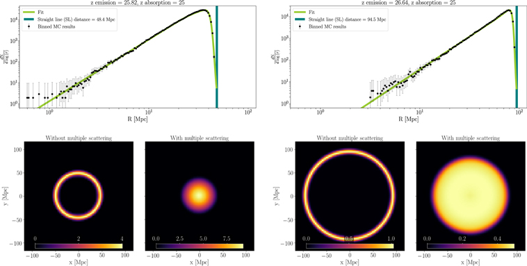
Figure 1. Calculation of the multiple scattering of Ly-α photons. Top panels: example distributions of the distance from the source at which photons are absorbed at the Ly-α frequency, given an emitted and absorbed redshift, generated using a photon-scattering Monte Carlo code. The black dots show the number of photons per bin of log distance, as obtained by the Monte Carlo code, for a total of 250,000 photons per panel. The light green line shows our fit to the distance distribution, while the dark green vertical line shows the straight-line distance that all these photons would have traveled without the effect of multiple scattering. Bottom panels: the corresponding window functions that are used in our seminumerical simulation of the 21 cm signal. The window function represents the distribution of photons per volume emitted from a point source at the center (normalized for display purposes to a volume integral of 106). Multiple scattering substantially changes the window functions from the previously used spherical shell window functions, which are shown for comparison. All panels show photons emitted and absorbed at specific redshifts: for all panels, zabsorption = 25, with zemission = 25.82 for the panels on the left and zemission = 26.64 on the right. Fully incorporating these window functions into our code and exploring a wide range of possible astrophysical parameters allows us to go well past previous investigations of the effect of Ly-α scattering (Chuzhoy & Zheng 2007; Semelin et al. 2007; Naoz & Barkana 2008; Vonlanthen et al. 2011; Higgins & Meiksin 2012).
Download figure:
Standard image High-resolution imageFigure 2 further shows a representative example of the distribution of Ly-α photons around a galaxy at z = 20. Compared with Figure 1, here we integrate over the emission redshift. We assume a radiation intensity as a function of redshift that follows the mean SFR taken from an example simulation. We see that multiple scattering results in a steeper radial profile.
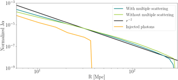
Figure 2. Representative example for the distribution of Ly-α photons around a galaxy at z = 20. The blue and green lines show continuum photons (i.e., photons emitted between the Ly-α and Ly-β frequencies, with and without the effect of multiple scattering). The orange line shows injected photons (coming from higher frequencies), for which the effect of multiple scattering is negligible. We also show an r−2 profile with the black line, for reference. Note that the y-axis covers many orders of magnitude, so even differences that appear small here can make a big difference.
Download figure:
Standard image High-resolution imageWe note that only in our group have the seminumerical simulations since early on (Fialkov et al. 2014a) included a rough approximation of the effect of multiple scattering on the 21 cm power spectrum, based on an analytical study (Naoz & Barkana 2008); while this did boost the power spectrum, we have now found that it underestimated the boost by a typical factor of 1.5 and did not capture the correct dependence on wavenumber or on the astrophysical parameters. We also note that while X-ray heating and UV ionizing radiation do not play a significant role in the 21 cm signal at the early times that we have focused on, these effects are included in our seminumerical simulations. We discuss the effect of introducing Poisson fluctuations into our simulation on the lower-redshift heating and reionization transitions in Reis et al. (2022). Ly-α photons themselves can contribute to the heating of the IGM, but this effect is small during cosmic dawn, as shown previously (Furlanetto & Pritchard 2006) and as we have also verified with our simulation (Reis et al. 2021; but note that Ly-α heating can become important at later redshifts, when the Ly-α intensity field is significantly larger than required to produce the Wouthuysen–Field effect).
3. Results
In this work, we present the combined effect of Poisson fluctuations and the multiple scattering of Ly-α photons on the 21 cm signal, over a wide range of astrophysical parameters that have never been probed this realistically before. Including these effects in our simulation, we obtain a cosmic-dawn 21 cm signal that is substantially different from previous predictions without these effects (Figure 3; see Figure 7 in Appendix A for another example, which shows that the effect remains striking even with halos of significantly lower mass). We clarify that by “previous work” we henceforth refer to models run with the same parameters as our full case, but including neither Poisson fluctuations nor multiple scattering (above we cited previous publications relating to these effects and laid out in detail their limitations).
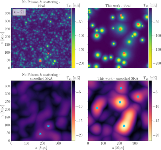
Figure 3. Simulated images of the cosmic-dawn 21 cm signal. Since early galaxies in this model are rare, we find it useful to show a kind of projected image, defined as showing the minimum value of the signal in the direction perpendicular to the image (obtained from a simulation box that is 384 comoving Mpc on a side; each image is made of square pixels of side 3 Mpc). All panels correspond to the same simulated volume, which illustrates a model with a star formation efficiency f⋆ = 0.1 and a minimum circular velocity Vc = 50 km s−1, corresponding to a minimum star-forming halo mass of Mmin ∼ 8 × 10⁸ M⊙ at the redshift shown, z = 21 (Figure 7 shows similarly striking effects for Vc = 25 km s−1). Left panels: the results from previous work, that is, without the effects of Poisson fluctuations and multiple scattering, shown on the scale set by the right-hand panels, for easy comparison. Right panels: the results from this work. Top panels: ideal images (i.e., showing the direct simulation outputs). Bottom panels: projections of the same simulated volumes as in the top panels, but as mock SKA images (see the text); such a smoothed projection can similarly be obtained from real images. In this work, the signal is composed of large “coupled bubbles” around individual galaxies. The large sizes and depths of the bubbles help them retain sufficient contrast in the mock SKA projected image to enable their detection. The locations of the > 3σ peaks as found in the smoothed SKA box are marked in both the ideal and SKA boxes, for easy comparison. The peaks correspond to individual coupled bubbles in the ideal image, while in the SKA box there is a minor contribution smoothed in from nearby smaller bubbles. Note that some additional peaks with lower significance can be seen in the SKA box, corresponding to smaller coupled bubbles in the ideal image. Also note that the SKA boxes are shown with respect to the cosmic mean brightness temperature, but the plotted values are negative, due to our choice of showing projected minimum values.
Download figure:
Standard image High-resolution imageIn the results corresponding to previous work, all simulation voxels produced a nonzero contribution to the Ly-α intensity field, but with Poisson fluctuations taken into account, at these high redshifts only a small fraction of voxels contain star-forming halos (initially only one per voxel). The stellar Ly-α photons produce coupling between the spin temperature and the kinetic gas temperature, and produce a 21 cm absorption halo around each star-forming halo. If we increase the Ly-α intensity (which corresponds to increasing the galaxy brightness), the 21 cm signal approaches saturation as the spin temperature approaches the kinetic temperature of the gas. Once this limit is reached near a halo, further increasing the Ly-α intensity cannot make the nearby absorption even deeper, but it does increase the size of the coupled bubble around the halo, which makes the bubble easier to observe. Meanwhile, the disappearance of halos from many pixels (where the previous fractional numbers of halos became zero after the implementation of Poisson fluctuations) clears out the regions between the bubbles, further increasing their relative contrast.
In order to study the observational consequences of a cosmic-dawn signal dominated by individual coupled bubbles, as described above, we used the SKA (Koopmans et al. 2015) as an example target instrument, and created mock SKA images that account for the expected angular resolution, thermal noise, and foreground effects, all as a function of redshift. There are two common approaches to dealing with the bright foreground expected in 21 cm images. Foreground removal involves modeling the foreground in order to subtract it accurately from the images (often with the help of additional observations obtained at higher resolution than needed for the cosmological 21 cm signal itself), while foreground avoidance involves removing regions in k-space that are expected to be contaminated by the foreground. Recent work (Datta et al. 2010; Dillon et al. 2014; Pober et al. 2014; Pober 2015) has shown that the foreground is expected to contaminate a wedge-like region in the k∣∣ versus k⊥ plane (where we separate the wavevector to components parallel and perpendicular to the line of sight), with more foreground-free k∣∣ modes available at lower k⊥ values. Since the SKA is designed to produce high-resolution deep-sky images, we assume that foreground subtraction will allow the remaining wedge of foreground avoidance to be relatively small. We refer to this reduced foreground avoidance, assumed to result from combining it with reasonably accurate foreground subtraction, as mild foreground avoidance. To the SKA images we then add a first analysis step of three-dimensional spherical smoothing, which we find to be helpful for reducing the noise (Banet et al. 2021) and bringing out the Ly-α bubbles.
A cosmic-dawn signal dominated by coupled bubbles is predicted to feature prominently in the 21 cm power spectrum (Figure 4), producing a distinct power-spectrum shape that is strongly correlated with the typical size of the bubbles (and thus the typical brightness of early galaxies). Coupled bubbles of size Rbubble suppress fluctuations on scales smaller than the typical bubble size, and thus result in a break in the power spectrum at kbreak ∼ 2π/Rbubble. Meanwhile, on large scales, the power spectrum is boosted compared to previous predictions by a factor that is between 2 and 7, depending on the astrophysical parameters. Thus, the signature of discrete galaxies is also a promising goal for radio arrays targeting the 21 cm power spectrum at cosmic dawn, such as HERA (Kohn et al. 2019) and NenuFAR (Zarka et al. 2012).
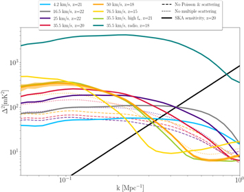
Figure 4. The 21 cm power spectrum at cosmic dawn. We show the power spectrum at the Ly-α peak (defined as the redshift at cosmic dawn where the power spectrum at k = 0.1 Mpc−1 peaks), for various cases with or without the effects of Poisson fluctuations and the multiple scattering of Ly-α photons (the solid lines and dashed lines, respectively). Unlike the gradual decline with k as previously expected (the dashed lines, shown in three cases: Vc = 25, 35.5, and 50 km s−1), we find a strong enhancement of the fluctuations on large scales (small k) and a clear break in the power spectrum. The break location corresponds to the typical size of the coupled bubbles, which in turn correlates strongly with the typical brightness of individual galaxies. If the power spectrum can be measured with a noise level that approaches the expected thermal noise of the SKA (the black line at z = 20), then the break may be detectable even if star formation occurred in halos as small as Vc ∼ 25 km s−1 (corresponding to Mmin = 1.1 × 10⁸ M⊙ at z = 20). We also show examples of including Poisson fluctuations, but not the multiple scattering of Ly-α photons (the dotted lines, corresponding to the same models as the dashed lines); both effects play a substantial role in the results shown in this work, with multiple scattering having a larger relative role in models with the lowest Mmin. For example, for the intermediate case of Vc = 35.5 km s−1 (which corresponds to 10 times the minimum mass for atomic cooling, or a minimum halo mass of Mmin ∼ 3 × 10⁸ M⊙ at z = 20), the power spectrum at k = 0.1 is enhanced by a factor of 3.8 compared to previous work, while Poisson fluctuations alone would produce an enhancement by a factor of 2.2. We also show one excess radio model motivated by the EDGES measurement (see the text). For all cases shown, the power spectrum was averaged over 18 different runs of the simulation, with different initial conditions and (for relevant cases) Poisson realizations. For the Vc = 50 km s−1 model, we also show the run-to-run variance with the shaded region. The SKA field-of-view variance is expected to be smaller, since the field of view (plus bandwidth) is larger than our simulation box.
Download figure:
Standard image High-resolution imageWhile it will be intriguing to detect individual coupled bubbles in 21 cm images (as illustrated in Figure 3), it is important to also construct an effective statistic, to be applied to 21 cm images of cosmic dawn, that aggregates together the individual bubbles and takes advantage of this feature in order to distinguish among models. We propose the total peak profile statistical probe, which measures a combination of the abundance, spatial extent, and brightness temperature depth of the coupled 21 cm bubbles. We first detect both minima and maxima in the smoothed SKA box (see Appendix A); an example of such detected peaks is shown in Figure 3 (only the peak minima are shown in the figure, for comparison with the image that shows the projected minimum values of the signal). We restrict ourselves to strong peaks, defined as having a value higher (in absolute value) than 3σ, where σ is the standard deviation of the SKA box voxel values. We calculate the radial profile around each peak that passes this threshold, and sum the profiles. The summing is done with the signed (that is, not absolute) value, in order to explicitly capture the asymmetry between the maxima and minima. Indeed, any symmetric field (about its mean) would give a total result approaching zero; thus, this statistic is inherently non-Gaussian, and naturally brings out the effect of individual galaxies over thermal noise and over any Gaussian component of the 21 cm fluctuations. Also, we sum (rather than average) these peak profiles, in order to maintain the sensitivity to the number density of the peaks. In order to avoid a direct dependence on the size of the observed volume, we normalize the result by scaling it to a volume of 1 Gpc3 (which corresponds almost exactly to the volume of an SKA field of view at z = 20 with a depth of 10 MHz, or to 18 of our simulation volumes). The resulting total peak profile per volume,  , is expected to be negative during the coupling era of cosmic dawn, and measuring it as such would imply stronger minima than maxima, thus confirming the detection of coupled bubbles of 21 cm absorption above the noise level. Figure 5 shows
  as calculated from the SKA boxes for a variety of possible parameters of early galaxies. The expected scatter in
  due to cosmic variance and noise, for an SKA field of view, is fairly small and is shown in Appendix B (Figure 6).
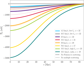
Figure 5. The total peak profile at cosmic dawn. We show the total radial profile around peaks,  , calculated from our simulated SKA data as a sum over all peaks, which is then normalized per Gpc3. Negative
  corresponds to the detection of coupled bubbles in 21 cm absorption on top of the SKA noise and foreground. A noise-dominated image (or any Gaussian signal) would instead give a result near zero. We show
  for the same astrophysical cases as in Figure 4. For each case, the redshift with the highest value of
  at r = 0 is shown. We obtain significant values of
  for a wide variety of astrophysical cases. The most prominent
  is seen for cases with higher star formation efficiencies and minimum masses for star formation. Such models produce larger and rarer (and thus higher-contrast) coupled bubbles. In results corresponding to previous work,
  is weaker (in absolute value) by a factor of 2–4, with Poisson fluctuations playing the dominant role in producing the large
  obtained in this work. With Poisson fluctuations included, the prominent peaks have such a high Ly-α intensity that their surroundings are already strongly coupled, even without accounting for multiple scattering, so that the additional effect of multiple scattering on their 21 cm profile is small; however, multiple scattering consistently has a strong effect on less prominent, more typical fluctuations, as measured by the 21 cm power spectrum (Figure 4; see also Figure 7). For each case shown, we averaged the results obtained from 18 different runs of the simulation, with independent realizations of the initial conditions, Poisson fluctuations, and SKA noise. For further discussion, see Appendix A.
Download figure:
Standard image High-resolution image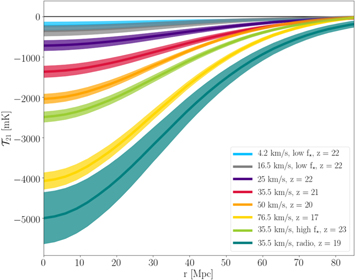
Figure 6. The scatter in the total peak profile. This plot is the same as Figure 5, but it also shows the scatter (only for this work, with all the new physical effects included). The scatter originates from both cosmic variance (which in turn originates from both the density field realization and the Poisson realization of the dark matter halos) and SKA noise. For each case shown, we calculated the standard deviation of the radial profile using our 18 simulation boxes, and then scaled the result to correspond to the scatter in an SKA field of view. This is shown for each case, with a colored region centered around the mean value.
Download figure:
Standard image High-resolution imageSince 21 cm coupling requires a quite low Ly-α intensity (Madau et al. 1997), it is expected to occur early enough that the observational probes considered here should be nearly unaffected (Cohen et al. 2018) by other astrophysical radiation, such as Ly-α heating, X-ray heating, or UV ionizing radiation; indeed, we have focused on signatures that occur early on, well before Ly-α coupling approaches saturation. This means that observations at this early time depend only on the mass distribution and star formation efficiency of halos. Higher masses of star-forming halos and higher star formation efficiencies increase the sizes of individual Ly-α bubbles, making it easier to detect them, as well as the corresponding power-spectrum break (which is moved to lower k). Now, higher halo masses also delay star formation and push the Ly-α peak to a lower redshift (where observations are easier), while high efficiencies go the other way. Overall, the masses and star formation efficiencies of star-forming halos can be deduced separately, given the multiple measures available, namely the amplitude and shape of the power spectrum and of the total peak profile, plus the redshifts at which these statistics peak (or, more generally, their redshift evolution).
In both Figures 4 and 5, we have included a case motivated by the recent, intriguing, but not yet independently verified EDGES measurement of the sky-averaged 21 cm signal from cosmic dawn (Bowman et al. 2018). The EDGES measurement implies a larger than expected ratio between the background radiation and gas temperatures at cosmic dawn. This can be explained either with a lower than expected kinetic gas temperature, due to a baryon–dark matter interaction (Barkana 2018; Muñoz & Loeb 2018; Liu et al. 2019), or an excess radio background that raises the effective radiation temperature (Bowman et al. 2018; Feng & Holder 2018; Fialkov & Barkana 2019). We include here an example of the latter model (Fialkov & Barkana 2019), with parameters that are consistent with the amplitude of the absorption detected by EDGES. If such an excess radio background exists, it should give the Ly-α bubbles a much higher contrast (>1000 mK), making them even more prominent in the SKA boxes, and more easily detectable through the total peak profile  , as well as the break in the 21 cm power spectrum (which is boosted tremendously in this case). We note that here we have assumed a uniform radio background (Fialkov & Barkana 2019), but if the excess radio radiation were to be emitted by the same galaxies that emitted the Ly-α radiation and created the bubbles, then the radio intensity should be higher near the galaxies, thus creating an even stronger contrast for the coupled bubbles (Reis et al. 2020).
4. Summary
In this work, we have presented the results of an upgraded simulation of the 21 cm signal from cosmic dawn, and discussed the implications for planned experiments, such as SKA or HERA. We introduced two new effects into our simulation: Poisson fluctuations in the number of galaxies and the multiple scattering of Ly-α photons. Compared to the results neglecting these effects, we found a 21 cm signal with enhanced contrast, showing the signatures of individual galaxies. In particular, the 21 cm power spectrum is enhanced by a factor of 2–7 on large scales, with a significantly different shape. Simulating SKA images, we found that it should be possible to detect individual galaxies at cosmic dawn, depending on the astrophysical scenario and advancements in data analysis techniques. We also discussed the total peak profile—an effective statistic that could be applied to future observations to distinguish between models.
For simplicity, we have assumed in this work a constant value of the star formation efficiency f⋆ for all star-forming halos. While this approach is common, in reality we expect significant scatter in the f⋆ value among galaxies, due to different merger and accretion histories, and as found in simulations (Xu et al. 2016). We have tested the effect of a galaxy-to-galaxy variance in the star formation efficiency, and found that a significant variance can strongly enhance the coupled bubble signature in the cosmic-dawn signal. Even for a lower average star formation efficiency than we have assumed, a variance in this parameter should still result in a few galaxies bright enough to produce large coupled bubbles that can be detected by the SKA. This highlights again the fact that the Ly-α bubble cosmic-dawn signal predicted here is produced by individual galaxies and affected by small number statistics at the tail of the brightness distribution. This is in contrast to previous work predicting a signal dominated by large-scale structure and determined by the average properties of the galaxy population. Our results are a boon to the planned 21 cm observations of cosmic dawn, as they predict favorable observational targets in the form of an enhanced 21 cm power spectrum and a strongly non-Gaussian 21 cm signal, even if most star-forming halos prove to be small, as is generally expected. Finally, we note that the novel effects investigated here also affect the global 21 cm signal (due to the nonlinearity of the 21 cm fluctuations), but only marginally, at the few to 10% level at the redshifts investigated here.
We acknowledge the usage of the DiRAC HPC. A.F. was supported by the Royal Society University Research Fellowship. This project was made possible for I.R. and R.B. through the support of the ISF-NSFC joint research program (grant No. 2580/17) and the Israel Science Foundation (grant No. 2359/20). R.B. also acknowledges the support of the Ambrose Monell Foundation and the Institute for Advanced Study.
This research made use of: SciPy (including pandas and NumPy; van der Walt et al. 2011; Virtanen et al. 2020), IPython (Pérez & Granger 2007), matplotlib (Hunter 2007), Astropy (Astropy Collaboration et al. 2013), Numba (Lam et al. 2015), the SIMBAD database (Wenger et al. 2000), and the NASA Astrophysics Data System Bibliographic Services.
Appendix A: SKA Boxes and Peak Detection
In order to simulate mock SKA images, we apply the following procedure to the ideal images that are directly output from our seminumerical simulations. (i) We smooth the ideal images with a two-dimensional Gaussian that corresponds approximately to the effect of SKA resolution. (ii) We add to the image a random realization of the SKA thermal noise, a pure Gaussian noise smoothed with the SKA resolution. The amplitude of the noise depends on the redshift and the SKA resolution. (iii) To account for the effects of the foreground, we adopt mild foreground avoidance.
The SKA is designed to be used at a range of different resolutions, depending on which ranges of baselines are included in the image. Higher resolution is not necessarily better, as it comes with higher noise. Here, we use a radius (corresponding approximately to half the FWHM of the point-spread function) of RSKA = 20 Mpc, since 10 Mpc seems too noisy, while 40 Mpc appears to wipe out too much of the signal (Banet et al. 2021); it may be useful to explore more systematically how the results of this work vary with this additional parameter, the resolution.
The strength of the SKA thermal noise (for a frequency depth corresponding to 3 comoving Mpc, and assuming a 1000 hour integration by the SKA) is approximately given by Koopmans et al. (2015) and Banet et al. (2021):

where the parameters a and b depend on the resolution used. For RSKA = 20 Mpc, which we use here, a = 4 mK and b = 5.1 gives a good fit for z > 16 (mainly of interest in this work), while for lower redshifts, b = 2.7.
As noted in the main text, foreground avoidance is the approach whereby the regions in k-space that are expected to be contaminated by foreground are removed. Assuming that the SKA will enable a first step of reasonably accurate foreground subtraction, our mild foreground avoidance assumes that the remaining wedge-like region will be relatively small. We assume that the remaining wedge that is still contaminated by foreground is given by k∣∣ < C(z)k⊥, where (Dillon et al. 2014; Jensen et al. 2015)
Here, RFoV is the angular radius of the field of view (for which we use the redshift-dependent value expected for the SKA) and DM is the (transverse) comoving distance. The model used here corresponds to an “optimistic model” from previous work (Pober et al. 2014). The real shape of the wedge is still under debate, and depends on advancements in analysis techniques. It is possible that foreground modeling and subtraction techniques will prove to produce better results than the foreground avoidance technique applied in this work.
To remove modes inside the wedge, we Fourier transform the 21 cm image (after two-dimensional smoothing and the addition of thermal noise), remove all modes inside the wedge, and inverse Fourier transform. To obtain the final SKA box that we use in the analysis, we further apply three-dimensional smoothing with a spherical top-hat of radius 20 Mpc (the same as the radius of the SKA angular resolution), as a first step in the analysis (not part of producing a mock SKA image). Since we are interested in spherically averaged peak profiles, it is sensible to add this smoothing in order to even out the differences between the angular directions (which suffer instrumental resolution smoothing) and the line of sight. More importantly, since the Ly-α bubbles are fairly large, we find that this step smooths out the thermal noise more than the signal, and thus brings out the bubbles (Banet et al. 2021).
Given the smoothed mock SKA boxes, we detect all maxima and minima, in order to calculate the total radial peak profile  . We then use a standard local peak detection algorithm implemented in scikit-image.
4
This simple approach for detecting the peaks is applicable here, since the SKA images are smooth (especially after the additional three-dimensional smoothing, which makes things more robust). We validated the results by visual inspection.
. We then use a standard local peak detection algorithm implemented in scikit-image.
4
This simple approach for detecting the peaks is applicable here, since the SKA images are smooth (especially after the additional three-dimensional smoothing, which makes things more robust). We validated the results by visual inspection.
As shown in the main text,  is a useful probe of the 21 cm signal. We note here a few additional points regarding this quantity. Its scatter as expected for an SKA field of view is shown in Figure 6; the scatter is small enough that it should not make it hard to distinguish among models with significantly different values of the minimum circular velocity Vc
of star-forming halos, except for the very lowest values (16.5 km s−1 and below). Also,
is a useful probe of the 21 cm signal. We note here a few additional points regarding this quantity. Its scatter as expected for an SKA field of view is shown in Figure 6; the scatter is small enough that it should not make it hard to distinguish among models with significantly different values of the minimum circular velocity Vc
of star-forming halos, except for the very lowest values (16.5 km s−1 and below). Also,  is a relative quantity, in the sense that it is sensitive to the number of peaks higher than three standard deviations of the signal. The standard deviation is sometimes dominated by thermal noise, but in many cases the (smoothed) original signal and foreground effects play more important roles. For this reason, we have used the standard deviation of the total mock signal, and not just that of the thermal noise, in the definition of
  . Deeper peaks produce a higher standard deviation through the foreground residuals resulting from mild foreground avoidance. In some cases, the positive peaks in the SKA boxes are not due to thermal noise, but due to these artifacts originating from foreground avoidance, with an amplitude that tends to correlate with the strength of the 21 cm signal. All of this reduces the differences among models with different parameters. It is possible that a more elaborate foreground removal algorithm would improve this behavior; to give one example idea, the highest detected peak could be fitted, and then the foreground residuals resulting from it could be removed approximately from the image, before the analysis continues onward, peak by peak. Finally, we note that while we have found that a threshold of three standard deviations works well, this is really an additional parameter of this statistic that can be further studied.
Appendix B: Low-Vc Example
In Figure 7, we show simulated images of cosmic dawn, similar to Figure 3, only for a model with lower-mass galaxies. This example shows that the signatures of individual massive galaxies can possibly be seen even in models with many star-forming low-mass galaxies.
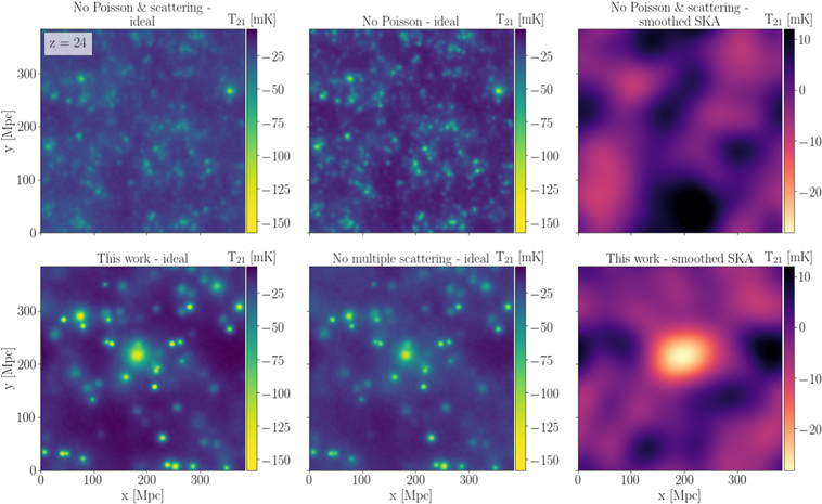
Figure 7. Simulated 21 cm images of cosmic dawn for a model in which small galaxies dominate. This is similar to Figure 3, but for Vc = 25 km s−1 (corresponding to a minimum star-forming halo mass of Mmin ∼ 8 × 10⁷ M⊙ at z = 24) and f⋆ = 0.1. Given the higher galaxy density in this model, here we show a thin (one-voxel) slice, and not a projection, as in Figure 3. For physical understanding, we also show intermediate cases (for the ideal image) that include only multiple scattering (no Poisson) or only Poisson fluctuations (no multiple scattering). Multiple scattering concentrates the Ly-α photons near sources, making the 21 cm peaks brighter (in absolute value) and the low-intensity regions darker. Even in an astrophysical scenario with many low-mass star-forming galaxies, Poisson fluctuations in the numbers of rare high-mass galaxies can still produce a large observable effect. In this example, a coupled bubble produced (mainly) by an individual massive halo (∼9 × 10⁸ M⊙) is seen. The coupled bubble is visible on top of a 21 cm signal otherwise dominated by low-mass galaxies, and is prominently seen in the SKA image (while nothing similar is seen in the version from previous work). For the astrophysical model shown here, a few such Ly-α bubbles are expected within an SKA field of view.
Download figure:
Standard image High-resolution imageFootnotes
- 4
scikit-image.org