Abstract
Detection of the IceCube-170922A neutrino coincident with the flaring blazar TXS 0506+056, the first and only ∼3σ high-energy neutrino source association to date, offers a potential breakthrough in our understanding of high-energy cosmic particles and blazar physics. We present a comprehensive analysis of TXS 0506+056 during its flaring state, using newly collected Swift, NuSTAR, and X-shooter data with Fermi observations and numerical models to constrain the blazar’s particle acceleration processes and multimessenger (electromagnetic (EM) and high-energy neutrino) emissions. Accounting properly for EM cascades in the emission region, we find a physically consistent picture only within a hybrid leptonic scenario, with γ-rays produced by external inverse-Compton processes and high-energy neutrinos via a radiatively subdominant hadronic component. We derive robust constraints on the blazar’s neutrino and cosmic-ray emissions and demonstrate that, because of cascade effects, the 0.1–100 keV emissions of TXS 0506+056 serve as a better probe of its hadronic acceleration and high-energy neutrino production processes than its GeV–TeV emissions. If the IceCube neutrino association holds, physical conditions in the TXS 0506+056 jet must be close to optimal for high-energy neutrino production, and are not favorable for ultrahigh-energy cosmic-ray acceleration. Alternatively, the challenges we identify in generating a significant rate of IceCube neutrino detections from TXS 0506+056 may disfavor single-zone models, in which γ-rays and high-energy neutrinos are produced in a single emission region. In concert with continued operations of the high-energy neutrino observatories, we advocate regular X-ray monitoring of TXS 0506+056 and other blazars in order to test single-zone blazar emission models, clarify the nature and extent of their hadronic acceleration processes, and carry out the most sensitive possible search for additional multimessenger sources.
1. Introduction
High-energy (HE;  ) neutrinos, as cosmic messenger particles, have the potential to reveal the sources of HE cosmic rays and illuminate their underlying particle acceleration processes. Detection of a nearly isotropic flux of HE cosmic neutrinos has been reported by the IceCube Collaboration (Aartsen et al. 2013a, 2013b); the absence of any identified point sources (Aartsen et al. 2016b) places firm limits on possible contributions from persistently bright neutrino sources (Murase & Waxman 2016). In this context, multimessenger studies have provided important clues to the origins of the diffuse neutrino, γ-ray, and cosmic-ray backgrounds (Murase et al. 2013; Fang & Murase 2018), and offer a powerful approach for identifying transient or highly variable neutrino sources, including blazar flares (Dermer et al. 2014; Kadler et al. 2016; Petropoulou et al. 2016; Turley et al. 2016). Anticipating these and related opportunities, the Astrophysical Multimessenger Observatory Network (AMON18
) was founded to link global HE and multimessenger observatories together into a single network and to distribute relevant alerts to the community in real-time (Smith et al. 2013).
) neutrinos, as cosmic messenger particles, have the potential to reveal the sources of HE cosmic rays and illuminate their underlying particle acceleration processes. Detection of a nearly isotropic flux of HE cosmic neutrinos has been reported by the IceCube Collaboration (Aartsen et al. 2013a, 2013b); the absence of any identified point sources (Aartsen et al. 2016b) places firm limits on possible contributions from persistently bright neutrino sources (Murase & Waxman 2016). In this context, multimessenger studies have provided important clues to the origins of the diffuse neutrino, γ-ray, and cosmic-ray backgrounds (Murase et al. 2013; Fang & Murase 2018), and offer a powerful approach for identifying transient or highly variable neutrino sources, including blazar flares (Dermer et al. 2014; Kadler et al. 2016; Petropoulou et al. 2016; Turley et al. 2016). Anticipating these and related opportunities, the Astrophysical Multimessenger Observatory Network (AMON18
) was founded to link global HE and multimessenger observatories together into a single network and to distribute relevant alerts to the community in real-time (Smith et al. 2013).
Blazars—active galactic nuclei oriented with a relativistic jet pointing toward Earth—dominate the extragalactic γ-ray sky (Ackermann et al. 2015, 2016). Yet, despite a wealth of electromagnetic (EM) data, blazar radiation mechanism(s) remain unclear, with leptonic and (lepto)hadronic scenarios providing viable explanations (e.g., Boettcher et al. 2013). Since blazars and other jetted active galactic nuclei are proposed ultrahigh-energy cosmic-ray (UHECR;  ) accelerators (e.g., Murase et al. 2012), the question of hadronic acceleration in these sources has important broader implications, and information from HE neutrinos will likely be crucial to resolving these issues (Murase 2017).
The AMON_ICECUBE_EHE alert 50579430 (hereafter, IceCube-170922A) was identified by IceCube and publicly distributed via AMON and the Gamma-ray Coordinates Network (GCN) within  of its interaction in the Antarctic ice cap at 20:54:30.43 UT on 2017 September 22 (GCN/AMON NOTICE IceCube-170922A 2017). As with previous likely cosmic events, its location was soon targeted by multiple observatories covering a broad energy range. The Swift-XRT (Keivani et al. 2017) and Fermi Large Area Telescope (LAT; Tanaka et al. 2017) reported an association with a blazar, TXS 0506+056, which showed strong activity in LAT data beginning in 2017 April and significant X-ray variability during Swift monitoring observations. Broadband EM observations of this event, the significance of the blazar flare, and the high-energy neutrino coincidence are discussed in Aartsen et al. (2018a).
The present work is organized as follows. In Section 2, we present a comprehensive analysis of Fermi (γ-ray), NuSTAR (hard X-ray), Swift (X-ray, ultraviolet, optical), and X-shooter (ultraviolet, optical, near-infrared) observations of TXS 0506+056, using these data to construct the source spectral energy distribution (SED) over near-infrared to γ-ray energies for two epochs: a 30 day period centered around the time of the neutrino trigger (Ep. 1) and a 30 day period starting 15 days after the neutrino trigger (Ep. 2). In Section 3, we model the SED of TXS 0506+056 in the flaring phase (Ep. 1) by performing detailed radiative transfer calculations, focusing on leptonic and hadronic single-zone emission scenarios. We discuss the implications of our modeling results in Section 4, and conclude in Section 5.
Throughout the manuscript, we use the notation  as a shorthand for the quantity
  (with Q in cgs units) unless stated otherwise. We note that given its redshift z = 0.3365 (Paiano et al. 2018) and a consensus cosmology, the luminosity distance of TXS 0506+056 is
  Mpc.
Mpc.
2. Observations and Analysis
In this section, we review the IceCube detection of the IceCube-170922A neutrino and present observations and data analysis for EM follow-up observations from the Fermi (γ-ray), NuSTAR (hard X-ray), Swift (X-ray, ultraviolet, optical), and X-shooter (ultraviolet, optical, near-infrared) facilities. We note that while very high-energy ( GeV) γ-ray observations by multiple facilities have been reported (de Naurois & H.E.S.S. Collaboration 2017; Mukherjee 2017), including a first detection at these energies by MAGIC (Mirzoyan 2017), details are not yet publicly available. These constraints are not included in our analysis. Given our results, consistency of our models with Fermi data out to
  , and current uncertainties in the necessary extragalactic background light corrections for the source at these energies, we do not expect that inclusion of these constraints would alter our conclusions.
2.1. IceCube Data
IceCube-170922A was an EHE neutrino event (GCN/AMON NOTICE 2016) identified and distributed by the IceCube Observatory via AMON and GCN within  of its detection at 20:54:30 UT on 2017 September 22 (GCN/AMON NOTICE IceCube-170922A 2017). A refined localization was reported four hours later (Kopper & Blaufuss 2017): R.A. =
  degree, decl. =
  degree (J2000; 90% containment ellipse). The maximum likelihood neutrino position is R.A. 05°09m08
784, decl. +05°45′13
32 (J2000); see Figure 1 for an illustration of the initial and final localizations.
Figure 1. Swift-XRT follow-up of IceCube-170922A. X-ray exposure map resulting from the adopted 19-point tiling pattern centered on the initial IceCube neutrino localization is shown in grayscale, and the positions of all detected X-ray sources with red points. The red dashed circle shows the initial 90%-containment region. The red solid ellipse shows the updated 90%-containment region (Kopper & Blaufuss 2017). Grayscale levels indicate achieved exposure at each sky position, as shown by the color bar. White streaks are due to dead regions on the XRT detector caused by a micrometeroid impact (Abbey et al. 2006).
Download figure:
Standard image High-resolution imageEHE neutrino event reports include the neutrino arrival time, direction (R.A. and decl.), angular error (r50 for 50% containment; r90 for 90% containment), revision number, an estimate of the deposited charge, an estimate of the neutrino energy, the parameter signalness, and an estimate of the probability that the event was due to an astrophysical—rather than atmospheric—neutrino (Aartsen et al. 2017a). Real-time identification, localization, and reporting of IceCube HE neutrinos is enabled by software that has been in place at the South Pole since 2016 April (Aartsen et al. 2017a).
2.2. Swift-XRT Data
IceCube-170922A triggered the Neil Gehrels Swift Observatory in automated fashion via AMON cyberinfrastructure, resulting in rapid-response mosaic-type follow-up observations, covering a roughly circular region of sky centered on the prompt localization in a 19-point tiling that began 3.25 hr after the neutrino detection. This initial epoch of Swift observations spanned 22.5 hr and accumulated ≈800 s exposure per pointing. The mosaic tiling yielded coverage of a region with radius ≈08 centered on R.A. 05h09m08
784, decl. +05°45′13
32 (J2000), amounting to a sky area of 2.1 deg2. XRT data were analyzed automatically, as data were received at the University of Leicester, via the reduction routines of Evans et al. (2009, 2014). Nine X-ray sources were detected in the covered region down to a typical achieved depth of
 erg cm−2 s−1(0.3–10.0 keV). Figure 1 shows the exposure map for the 19-point tiling pattern, along with the nine detected X-ray sources. All detected sources were identified as counterparts to known and cataloged stars, X-ray sources, or radio sources (Keivani et al. 2017); fluxes of these X-ray sources were consistent with previously measured values.
Notably, Source 2 from these observations (marked as X2 on Figure 1), located 46 from the center of the neutrino localization, was identified by us as the likely X-ray counterpart to QSO J0509+0541, also known as TXS 0506+056. This was the first report to connect TXS 0506+056 to IceCube-170922A (Keivani et al. 2017).
Following the Fermi report that TXS 0506+056 was in a rare GeV-flaring state (Tanaka et al. 2017), we commenced a Swift monitoring campaign on September 27 (Evans et al. 2017). Swift monitored TXS 0506+056 for 36 epochs by November 30 with 53.7 ks total exposure time (Table 1).
Table 1. Swift-XRT Monitoring of TXS 0506+056
| Epoch | Exposure [ks] | Photon Index |

|

|
|---|---|---|---|---|
| (1) | (2) | (3) | (4) | (5) |
| 58019.4700 ± 0.4630 | 0.8 |

|
65.8 ± 10.1 |

|
| 58023.8535 ± 0.0660 | 4.9 | 2.43 ± 0.12 | 121.0 ± 5.3 |

|
| 58026.2273 ± 0.0391 | 2.0 | 2.30 ± 0.33 | 66.2 ± 7.8 |

|
| 58028.6419 ± 0.0114 | 2.0 | 2.73 ± 0.20 | 117.0 ± 8.2 |

|
| 58029.6745 ± 0.1036 | 1.1 |

|
182.0 ± 14.1 |

|
| 58030.7369 ± 0.0385 | 1.2 |

|
186.0 ± 16.1 |

|
| 58031.7944 ± 0.1025 | 2.3 | 2.64 ± 0.13 | 255.0 ± 11.7 |

|
| 58032.8985 ± 0.3428 | 2.1 |

|
90.1 ± 7.1 |

|
| 58034.4478 ± 0.0337 | 1.9 | 2.53 ± 0.21 | 108.0 ± 8.1 |

|
| 58040.9452 ± 0.0010 | 0.2 |

|

|

|
| 58042.7684 ± 0.1686 | 2.2 | 2.00 ± 0.27 | 61.9 ± 5.8 |

|
| 58044.1300 ± 0.0696 | 1.8 | 2.10 ± 0.31 | 52.6 ± 6.0 |

|
| 58047.2130 ± 0.6360 | 2.3 | 2.11 ± 0.28 | 49.6 ± 5.1 |

|
| 58050.7286 ± 0.0446 | 2.9 |

|
46.6 ± 4.4 |

|
| 58053.3162 ± 0.0335 | 1.0 |

|
54.4 ± 8.2 |

|
| 58059.6620 ± 0.0729 | 3.3 | 2.22 ± 0.21 | 60.2 ± 4.7 |

|
| 58065.6390 ± 0.3371 | 3.1 | 2.30 ± 0.20 | 83.4 ± 6.2 |

|
| 58068.3642 ± 0.0742 | 3.0 | 2.38 ± 0.24 | 55.7 ± 4.9 |

|
| 58069.5359 ± 0.5032 | 1.8 | 2.23 ± 0.24 | 83.3 ± 7.5 |

|
| 58071.1551 ± 0.1299 | 2.9 | 2.15 ± 0.19 | 81.1 ± 5.9 |

|
| 58072.0949 ± 0.0039 | 0.7 |

|
48.5 ± 9.1 |

|
| 58073.0911 ± 0.0042 | 0.7 |

|
55.0 ± 9.7 |

|
| 58074.2484 ± 0.0962 | 3.0 |

|
54.4 ± 4.8 |

|
| 58075.0831 ± 0.0046 | 0.8 | 2.51 ± 0.45 | 63.1 ± 9.6 |

|
| 58075.6655 ± 0.0057 | 1.0 | 1.94 ± 0.41 | 60.6 ± 9.4 |

|
| 58076.0793 ± 0.0049 | 0.8 |

|
56.1 ± 9.0 |

|
| 58077.0756 ± 0.0054 | 0.9 |

|
61.4 ± 8.9 |

|
| 58078.0717 ± 0.0056 | 1.0 |

|
40.5 ± 7.1 |

|
| 58079.0675 ± 0.0057 | 1.0 |

|
49.3 ± 8.6 |

|
| 58080.1320 ± 0.0057 | 1.0 |

|
47.4 ± 9.4 |

|
| 58081.1279 ± 0.0057 | 1.0 |

|
45.8 ± 9.7 |

|
| 58082.0551 ± 0.0057 | 1.0 |

|

|

|
| 58083.1195 ± 0.0057 | 1.0 | 2.45 ± 0.56 | 44.4 ± 8.0 |

|
| 58084.0499 ± 0.0058 | 1.0 |

|
39.0 ± 6.9 |

|
| 58086.1089 ± 0.0059 | 1.0 |

|
45.4 ± 9.8 |

|
| 58087.1560 ± 0.0053 | 0.9 |

|
66.9 ± 9.2 |

|
Note.  and
and  indicate count rate and energy flux, in units of 10−3 ct s−1and 10−12 erg cm−2 s−1, respectively. Uncertainties are quoted at 90% confidence.
Download table as: ASCIITypeset image
To characterize the X-ray flux and spectral variability of TXS 0506+056, we performed a power-law fit to each individual Swift-XRT observation (Table 1), as well as to the summed spectrum from all listed epochs, using XSPEC (Arnaud 1996). The observation on October 14 is excluded from the spectral analysis due to low exposure time. The summed spectrum is adequately fit with a single power-law spectral model having the Galactic column density  cm−2, resulting in a photon index
  and mean flux of
  erg cm−2 s−1 (0.3–10.0 keV).
We note that this source has been observed on multiple previous occasions with Swift-XRT, with results published in the 1SXPS catalog (Evans et al. 2014). In past observations, TXS 0506+056 exhibited a typical flux of  erg cm−2 s−1, with one observation at
  erg cm−2 s−1(0.3–10.0 keV). The source was thus in an active X-ray flaring state by comparison to historical X-ray measurements (Figure 2, upper left). Photon indices and X-ray flux measurements for each epoch are provided in Table 1, and the variations in photon index are shown in Figure 2 (upper right). The Swift-XRT light curve is shown in Figure 2 (upper left).

Figure 2. (Left top) Swift-XRT light curve. Each bin corresponds to one observation in the 0.3–10 keV energy range. The horizontal bands show the XRT historical data (four observations) of TXS 0506+056: the mean historical quiescent flux from combining three data points, and one showing the rate from the outburst observation. (Left bottom) Swift-UVOT light curve for all 36 observations performed on TXS 0506+056. The dashed line shows the IceCube-170922A arrival time. (Right top) Swift-XRT photon index variation during the XRT monitoring campaign of TXS 0506+056. The solid horizontal line shows the photon index of the stacked X-ray spectrum over the 2 epochs, while the dashed lines represent the uncertainties. (Right bottom) Swift-UVOT photon index variations obtained from a power-law fit to the energy flux spectrum ( vs.
vs.  ). In all plots, Ep. 1 and Ep. 2 are, respectively, defined as [−15 days, +15 days] and [+15 days, +45 days] time windows with respect to the IceCube-170922A arrival time.
Download figure:
Standard image High-resolution image2.3. NuSTAR Data
To further characterize the HE emissions of the source, we requested two observations with the NuSTAR hard X-ray (3.0–100 keV) mission (Harrison et al. 2013).
On 2017 September 29 (02:23–17:48 UTC) NuSTAR carried out a Target of Opportunity observation of TXS 0506+056 (Fox et al. 2017). The full science observation was retrieved from the NuSTAR public archive (ObsID 90301618002). Data were processed within the HEAsoft (Arnaud 1996) software environment using the nupipeline tool with the setting SAAMODE=strict. This yielded exposures of 23.9 ks (24.5 ks) and count rates of 21.3 ct ks−1(20.8 ct ks−1) in the A (B) units, respectively. Level 3 data products for the source were then extracted using the nuproducts tool. Within XSPEC, spectral data from both units were fit to a single power-law model with  cm−2, resulting in a photon index of
  and a flux of
  erg cm−2 s−1 (3.0–79.0 keV).
On 2017 October 19 (10:26 to 21:21 UTC) NuSTAR performed a second Target of Opportunity observation of TXS 0506+056 (ObsID 90301618004). Executing the same reduction as for the first observation yielded exposures of 19.7 ks (19.7 ks) and count rates of 20.2 ct ks−1(19.6 ct ks−1) in the A (B) units at this second epoch. Performing the same spectral fit as for the first observation, we obtain a photon index  and flux of
  erg cm−2 s−1 (3.0–79.0 keV), consistent with results of the first observation from 20 days earlier.
2.4. Joint Swift-XRT and NuSTAR Analysis
In order to obtain the energy spectrum for a wider X-ray band (0.2–100 keV), we simultaneously fit data from individual XRT observations and NuSTAR for two main epochs: [−15 days, +15 days] (Ep. 1) and [+15 days, +45 days] (Ep. 2) relative to the neutrino detection. The two epochs include eight and seven XRT observations, respectively, and one NuSTAR observation each. Since the source spectrum over the NuSTAR bandpass does not change from Ep. 1 to Ep. 2, we fit all individual XRT observations together with both NuSTAR observations with a sum of two power laws model, including Galactic absorption frozen at  cm−2, and quote the soft component best-fit parameters when reporting XRT results. A Markov Chain Monte Carlo algorithm is then employed for each fit to provide the 90% confidence levels. We generate 1000 realizations of the spectra from each XRT observation and add all Ep. 1 and Ep. 2 realizations together in order to find the 90% confidence intervals on the flux density versus energy. This joint analysis results in best-fit photon indices (
 ) of
) of  and
and  . The results are displayed in Figure 3 and used for subsequent SED modeling (see Section 3).

Figure 3. Observations and spectral energy distribution (SED) for TXS 0506+056 in its high-flux state. Left panel: timeline of observations by Fermi, Swift, NuSTAR, and X-shooter. Observations are divided into two 30 day epochs each for analysis and discussion purposes; the vertical dashed line shows the IceCube-170922A detection time. Right panel: multiwavelength SED for TXS 0506+056; data with the 90%-confidence bands on source emission are shown separately for the two epochs for each facility. The SEDs for Ep. 1 and Ep. 2 are broadly similar, with the source fading somewhat at optical through X-ray energies, and the ultraviolet/optical spectrum softening.
Download figure:
Standard image High-resolution image2.5. Swift UltraViolet and Optical Telescope (UVOT) Data
The Swift-UVOT (Roming et al. 2005) also participated in the rapid-response follow-up observations of the IceCube-170922A and the subsequent monitoring of the flaring blazar TXS 0506+056 as described in Section 2.2. The u filter was used during all 19 pointings used to tile the region around IceCube-170922A. TXS 0506+056 was readily detected during this initial survey. All six UVOT lenticular filters (v, b, u, uvw1, uvm2, uvw2) were used during the subsequent observations monitoring TXS 0506+056.
UVOT data were analyzed using the standard tool uvotsource of HEAsoft (v6.22.1) and the latest updates to the UVOT CALDB files. uvotsource does aperture photometry (Breeveld et al. 2010, 2011) using user-specified source and background regions. Because TXS 0506+056 is a bright source, a 5″ aperture was used for the source region. A nearby source-free region was used as the background region instead of the usual concentric ring centered on the target to avoid contamination from a read-out streak. The read-out streak is produced by photons from a very bright source near the edge of the UVOT image that arrive during the brief time in which the image frame is transferred for read out of the detector’s CCD (Page et al. 2013). The position of the read-out streak changes from observation to observation as the orientation on the sky of the UVOT image changes. Consequently, a different nearby background region was used for the observations centered near MJD 58065 (Swift sequence 00083368018). Data from observations near MJD 58028.6 (sequence 00083368003) and MJD 58031.8 (sequence 00083368006) are not used because the source region is within the read-out streak.
Table 2 reports the times, exposures, and magnitudes for all the observations. The source varies over a range of at least 0.5 mag in all six filters.
Table 2. Swift-UVOT Monitoring of TXS 0506+056
| Epocha (MJD) | Exposure (s) | Filter | Magnitudeb |
|---|---|---|---|
| (1) | (2) | (3) | (4) |
| 58019.4699 ± 0.4632 | 780 | u | 14.31 ± 0.03 |
| 58023.8555 ± 0.0641 | 809 | uvw2 | 14.58 ± 0.03 |
| 58023.8257 ± 0.0306 | 157 | v | 14.62 ± 0.04 |
| 58023.8364 ± 0.0403 | 2930 | uvm2 | 14.50 ± 0.03 |
| 58023.8515 ± 0.0639 | 472 | uvw1 | 14.36 ± 0.04 |
| 58023.8529 ± 0.0635 | 236 | u | 14.27 ± 0.04 |
| 58023.8539 ± 0.0635 | 236 | b | 15.08 ± 0.03 |
| 58026.2274 ± 0.0391 | 1954 | uvm2 | 14.81 ± 0.04 |
Notes.
aMJD at the middle of the observation. bErrors at 1σ uncertainty.Only a portion of this table is shown here to demonstrate its form and content. A machine-readable version of the full table is available.
Download table as: DataTypeset image
2.6. Swift-UVOT Analysis
Due to the UVOT’s blue response, extending as far as  Å, it is necessary to apply an appropriate extinction correction in order to interpret UVOT observations appropriately and derive physical constraints on the SED of TXS 0506+056. The line-of-sight extinction to TXS 0506+056, as provided by the NASA/IPAC Infrared Science Archive19
is AV = 0.286 mag according to all-sky dust maps (Schlegel et al. 1998; Schlafly & Finkbeiner 2011). Although this estimate nominally has little uncertainty (
Å, it is necessary to apply an appropriate extinction correction in order to interpret UVOT observations appropriately and derive physical constraints on the SED of TXS 0506+056. The line-of-sight extinction to TXS 0506+056, as provided by the NASA/IPAC Infrared Science Archive19
is AV = 0.286 mag according to all-sky dust maps (Schlegel et al. 1998; Schlafly & Finkbeiner 2011). Although this estimate nominally has little uncertainty ( mag), we note that (1) this quoted value has been corrected from the original published value by 14% (Schlafly & Finkbeiner 2011); and (2) a subsequent recalibration with a similar approach, using PanSTARRS-1 rather than Sloan Digital Sky Survey data (Green et al. 2015), leads to a different extinction estimate, AV = 0.254 mag. We therefore take a conservative approach and adopt a line-of-sight extinction of
 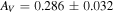 mag, with Gaussian form, as our prior for UVOT SED analysis. To calculate extinction as a function of wavelength, we use the Fitzpatrick (1999) extinction law with RV = 3.1.
On 1 occasion during Ep. 1, on 3 occasions during Ep. 2, and on 20 subsequent occasions before November 30, UVOT observations were carried out using all six UV/optical filters in rapid sequence. We use these observations to characterize the UV/optical SED and UVOT spectral index (Figure 2, lower right). Additional single-filter observations are then used (in tandem with the six-filter epochs) to estimate source variability (Figure 2, lower left).
To fit the SED for each six-filter UVOT observation, we perform a χ2 minimization of the predicted versus observed count rates in each filter using a model with three parameters: source flux density Fν at  Hz, UVOT spectral index β, and extinction AV. Extinction values away from our adopted value of AV = 0.286 mag are penalized according to our Gaussian extinction uncertainty. The source spectrum is integrated across each filter bandpass using the filter transmission function20
and Fitzpatrick (1999) extinction curve. A fit is considered successful if the total χ2 across the six filters gives a p-value
Hz, UVOT spectral index β, and extinction AV. Extinction values away from our adopted value of AV = 0.286 mag are penalized according to our Gaussian extinction uncertainty. The source spectrum is integrated across each filter bandpass using the filter transmission function20
and Fitzpatrick (1999) extinction curve. A fit is considered successful if the total χ2 across the six filters gives a p-value  . Only one of the six-filter observations (at δt = 64.5 days after IceCube-170922A) violates this constraint, and thus receives treatment as a broken power law across the UVOT filters (forcing a single power-law fit gives a spectral index β = 1.66 ± 0.06 at this epoch, where we quote uncertainties from
  analysis even though the fit is acknowledged not to be satisfactory). We note that curvature of the source spectrum (in particular, steepening/softening toward the UV) is also observed in the X-shooter data (Section 2.7). Acceptable fits yield a best-fit value for the UVOT spectral index and uncertainty via
  analysis. These values and uncertainties are reported in Table 3 and plotted in Figure 2 (lower right).
Table 3. Swift-UVOT Photon Indices for TXS 0506+056
| Epoch | Photon Index |
|---|---|
| 58023.7632 |

|
| 58050.6452 |

|
| 58053.2192 |

|
| 58059.5782 |

|
| 58065.5562 |

|
| 58068.2802 |

|
| 58069.9502 |

|
| 58070.9472 |

|
| 58072.0112 |

|
| 58073.0082 |

|
| 58074.1632 |

|
| 58074.9992 |

|
| 58075.5822 |

|
| 58075.9962 |

|
| 58076.9922 |

|
| 58077.9882 |

|
| 58078.9842 |

|
| 58080.0482 |

|
| 58081.0442 |

|
| 58081.9712 |

|
| 58083.9662 |

|
| 58086.0252 |

|
| 58083.0362 (UV) |

|
| 58083.0362 (Vis) |

|
| 58087.0722 |

|
Note. UVOT photon indices from power-law SED fitting for epochs with data in all six filters. Data for the next-to-last epoch are fitted with a power law to the three UV and three visible filters separately; a forced single power-law fit to this epoch yields a photon index of 2.66, see the text for details.
Download table as: ASCIITypeset image
We determine UVOT SED bands, the range of fluxes allowed at 90% confidence for each photon energy, by drawing 1000 samples according to the χ2 probability function, and generating a power-law spectrum across the UVOT bandpass for each. The allowed range at each energy in the SED is defined as the minimum-width range encompassing 90% of these spectra. For Ep. 2, we draw 1000 samples from each of the three six-filter epochs and combine these before finding the 90%-confidence range; results for this epoch thus account for source flux variability. For Ep. 1, we use only the single six-filter observation to characterize the SED; we estimate accounting for flux variability over Ep. 1 would expand this band by 12%; however, we do not make this correction in our analysis.
We determine UVOT fluxes for single-epoch observations using the β measurement from the temporally proximate six-filter observation, adjusting the flux density at 1015 Hz to achieve agreement with the observed count rate in the relevant filter. Quoted uncertainties for these flux estimates combine the Poisson count rate uncertainty with the uncertainty in flux for the adopted SED model, in quadrature. Flux values and uncertainties are reported in Table 4 and plotted in Figure 2 (lower left).
Table 4. Swift-UVOT Extinction-corrected Fluxes at ν = 1015 Hz
| Epoch |

|
|---|---|
| 58019.4709 | 22.50 ± 3.29 |
| 58023.8470 | 34.80 ± 3.13 |
| 58026.2284 | 12.80 ± 3.13 |
| 58029.6756 | 15.80 ± 3.13 |
| 58030.7380 | 15.00 ± 3.29 |
| 58032.5593 | 19.30 ± 3.29 |
| 58033.1319 | 11.00 ± 3.13 |
| 58034.4489 | 13.80 ± 3.29 |
| 58040.9463 | 16.00 ± 1.97 |
| 58042.7696 | 15.70 ± 1.97 |
| 58044.1311 | 19.60 ± 1.97 |
| 58046.5814 | 10.90 ± 1.97 |
| 58047.8132 | 13.70 ± 1.97 |
| 58050.7285 | 19.80 ± 1.81 |
| 58053.3030 | 22.40 ± 2.14 |
| 58059.6613 | 26.70 ± 2.47 |
| 58065.6395 | 24.70 ± 2.30 |
| 58068.3633 | 18.60 ± 1.81 |
| 58070.0338 | 19.40 ± 1.81 |
| 58071.0301 | 21.30 ± 2.14 |
| 58072.0950 | 22.70 ± 2.30 |
| 58073.0911 | 22.30 ± 2.14 |
| 58074.2466 | 24.70 ± 2.30 |
| 58075.0830 | 25.60 ± 2.47 |
| 58075.6651 | 23.70 ± 2.30 |
| 58076.0792 | 23.20 ± 2.14 |
| 58077.0751 | 23.80 ± 2.30 |
| 58078.0713 | 26.10 ± 2.47 |
| 58079.0670 | 24.70 ± 2.47 |
| 58080.1316 | 25.10 ± 2.47 |
| 58081.1274 | 24.60 ± 2.30 |
| 58082.0546 | 24.30 ± 2.30 |
| 58083.1191 | 21.40 ± 2.14 |
| 58084.0496 | 27.30 ± 2.63 |
| 58086.1085 | 30.10 ± 2.96 |
| 58087.1557 | 21.70 ± 2.80 |
Note.  is the
  flux at ν = 1015 Hz in units of 10−12 erg cm−2 s−1, derived by SED fitting for six-filter epochs, and adjusted to ν = 1015 Hz using the nearest best-fit SED index for single-filter epochs.
Download table as: ASCIITypeset image
2.7. X-shooter Data
Medium-resolution spectroscopy of TXS 0506+056 was obtained with the X-shooter spectrograph (Vernet et al. 2011) mounted on the Very Large Telescope UT2 at ESO Paranal Observatory on 2017 October 1. The three arms of X-shooter (UV: UVB, optical: VIS and near-infrared: NIR) were used with slit widths of 10, 0
9, and 0
9, respectively. These data provide simultaneous 300–2480 nm spectral coverage with average spectral resolutions
 of 4290, 7410, and 5410, respectively, in each arm. Observing conditions were good, with a clear sky, seeing of ∼0
8, and an airmass ranging from 1.2 to 1.3. Individual exposure times are 72, 139, and 54 s for the UBV, VIS, and NIR arms, respectively, and sum to total integration times of 1152, 2224, and 864 s. Standard ABBA nodding observing mode was used to allow for an effective background subtraction.
Data were reduced using the ESO X-shooter pipeline (Goldoni et al. 2006; Modigliani et al. 2010) (v.2.9.3) in the Reflex environment (Freudling et al. 2013), producing a background-subtracted, wavelength-calibrated spectrum. The extracted 1D spectrum was flux calibrated with the X-shooter pipeline using a response function produced by observing the HST white dwarf standard GD71 (R.A. 05h52m2786, decl. +15°53′13
8, J2000) just after the observation of TXS 0506+056. To correct results for slit losses, the final spectrum was rescaled to match the broadband B, V, and R magnitudes obtained on 2017 October 29 using the 1 m Kapteyn Telescope at La Palma (Keel & Santander 2017). Overall, the flux calibration is expected to be accurate to 10% in the UVB arm and 15% in both the VIS and NIR arms based on the seeing conditions at the observing time. The telluric absorption lines were removed by using the Molecfit software through a fit of synthetic transmission spectra calculated by a radiative transfer code (Kausch et al. 2015; Smette et al. 2015). Finally, we corrected the spectra for Galactic extinction using the extinction law of Fitzpatrick (1999) with a total extinction at the V filter band AV = 0.286 mag and a selective-to-total extinction ratio equal to the Galactic average value RV = 3.1. For the 90%-confidence band plotted in Figure 3, we allowed the extinction to vary by δAV = ± 0.054 mag, according to our adopted uncertainty (Section 2.6).
Two Galactic interstellar absorption features are observed in the reduced spectrum: Ca K and H absorption lines (at 3933.7 Å and 3968. Å respectively), and the Na ID doublet at 5892.5 Å. No other emission or absorption line is observed. Overall, the spectrum is consistent with the spectrum of a nonthermally dominated blazar and confirms the source to exhibit a bluer spectrum than that published by Halpern et al. (2003), as previously mentioned by Steele (2017).
Both the X-shooter and Swift-UVOT data clearly show that the synchrotron peak is below  Hz. This indicates that TXS 0506+056 is an intermediate synchrotron peaked (ISP) or low synchrotron peaked blazar.
The nondetection of Lyα absorption in the X-shooter spectrum provides a rough upper limit on the redshift of TXS 0506+056,  , which is compatible with the redshift measurement (z = 0.3365 ± 0.0010) of Paiano et al. (2018).
2.8. Fermi Data
The Fermi-LAT is a pair conversion telescope sensitive to γ rays in the 20 MeV to >300 GeV (Atwood et al. 2009). In this section, we analyze photons detected by the LAT during our defined Ep. 1 (±15 days from the neutrino detection) and Ep. 2 (15 to 45 days after the neutrino detection). Analysis was performed using version v10r0p5 of the Fermi Science Tools.21
Photons with energies between 100 MeV and 300 GeV that were detected within a radius of 15° from the location of TXS 0506+056 were selected for the analysis, while photons with a zenith angle  were discarded to reduce contamination from the Earth’s albedo.
The contribution from isotropic and Galactic diffuse backgrounds was modeled using the parameterization provided in the files iso_P8R2_SOURCE_V6_v06.txt and gll_iem_v06.fits, respectively. Sources in the 3FGL catalog within a radius of 15° from the source position were included in the model, with spectral parameters fixed to their catalog values, while spectral parameters for sources within 3° were allowed to vary freely during the fit. The TXS 0506+056 spectral fit was performed with a binned likelihood method using the P8R2_SOURCE_V6 instrument response function. A power-law fit to the spectrum gives a photon index of  , consistent with the 3FGL value of 2.04 ± 0.03, and a flux normalization of
  cm−2 s−1 MeV−1 at an energy of 1.44 GeV, about a factor of four higher than the 3FGL value of
  in the same units. The spectral fit was repeated in seven independent energy bins with equal logarithmic spacing in the 100 MeV–300 GeV range to be incorporated in the modeling of the SED. Best-fit flux values and 90% uncertainties, shown in Figure 3 and subsequent figures, are reported for spectral bins with a test statistic (TS) value larger than 9, which corresponds to an excess of ∼3σ. Flux upper limits at the 95% confidence level are quoted otherwise.
3. Multimessenger Modeling
Traditionally, blazar SEDs are interpreted in two different ways. In the leptonic scenario, the γ-ray component is interpreted as synchrotron self-Compton (SSC) emission or external inverse-Compton (EIC) emission (e.g., Maraschi et al. 1992; Dermer & Schlickeiser 1993; Sikora et al. 1994). In the SSC model, the seed photons for Compton scattering are produced internally in the blazar jet; in particular, these are the synchrotron photons produced by nonthermal electron–positron pairs accelerated in the jet. In the EIC model, the seeds for Compton scattering are provided by external radiation fields, such as scattered accretion disk radiation, broadline/dust emission, and soft radiation from the sheath region of a structured jet.
It is natural that protons and nuclei are also accelerated in the jet, leading to the so-called leptohadronic scenario22
where the γ-ray emission is explained by processes related to relativistic protons: proton-induced EM cascades (Mannheim 1993; Mücke et al. 2003), proton synchrotron emission (Aharonian 2000; Mücke et al. 2003), or intergalactic magnetic cascades induced by UHECRs (Essey et al. 2011; Murase et al. 2012). In the presence of relativistic protons, theory has predicted that PeV–EeV neutrinos can be produced via the photomeson production process between cosmic-ray protons and target photons provided by the intra-jet and/or external radiation fields (see Murase 2017 for a recent review on AGN neutrinos and references therein). For example, a neutrino with  –1 PeV implies a parent proton with energy
  ≈ 2.0–20 PeV, for which photomeson production mainly occurs with target photons with UV or greater energies.
HE neutrinos generated by photohadronic interactions must be accompanied by EM emission of secondary electron–positron pairs and pionic γ rays. EM cascades redistribute energy from high energies (e.g., PeV) to lower energies (e.g., keV–MeV) and exhibit  . These cascade effects are included in our detailed numerical calculations, as presented in the following sections.
3.1. Model Description
We assume that protons and electrons are coaccelerated by some mechanism, whose details lie outside the immediate scope of this work and are subsequently injected isotropically in a spherical region containing a tangled magnetic field. The particle interactions with the magnetic field and with secondary particles leads to the development of a system with five stable particle populations in steady state: protons, which lose energy by synchrotron radiation, Bethe–Heitler pair production, and photomeson production processes; electrons and positrons, which lose energy by synchrotron radiation and IC scattering; photons, which gain and lose energy in a variety of ways; neutrons, which can escape almost unimpeded from the source region, with a certain probability of photohadronic interactions; and neutrinos, which escape without any attenuation. The interplay of the processes governing the evolution of the energy distributions of those five populations is formulated with a set of time-dependent kinetic equations. Through them, energy is conserved in a self-consistent manner, since all the energy gained by a particle type has to come from an equal amount of energy lost by another particle type.
To simultaneously solve the coupled kinetic equations for all particle types, we use the time-dependent code described in Dimitrakoudis et al. (2012). Photomeson production processes are modeled using the results of the Monte Carlo event generator SOPHIA (Mücke et al. 2000), while the Bethe–Heitler pair production is similarly modeled with the Monte Carlo results of Protheroe & Johnson (1996) and Mastichiadis et al. (2005). The only particles that are not modeled with kinetic equations are muons, pions, and kaons (Dimitrakoudis et al. 2014; Petropoulou et al. 2014); their energy losses can be safely ignored for the parameter values relevant to this study (see also Murase et al. 2014 for numerical calculations where the kinetic equations for these particles are explicitly solved).
The parameters that describe the source (i.e., Doppler factor δ, comoving magnetic field strength B′, and comoving blob size R′) as well as those of accelerated (i.e., primary) particle distributions can often be constrained by multiwavelength data (Takahashi et al. 1996; Mastichiadis & Kirk 1997; Romanova & Lovelace 1997; Kirk et al. 1998; Li & Kusunose 2000); a complete list of model parameters is provided in Table 5.
Table 5. Physical Parameters (Description, Symbol, and Units) Used in Blazar Leptonic and Hadronic Modeling
| Parameter | Symbol | Unit [in cgs] |
|---|---|---|
| Doppler factor | δ | n/a |
| Magnetic field strength | B′ | G |
| Blob radius | R′ | cm |
| Electron injection luminosity |

|
erg s−1 |
| Minimum electron Lorentz factor |

|
n/a |
| Maximum electron Lorentz factor |

|
n/a |
| Break electron Lorentz factor |

|
n/a |
| Power-law electron index below the break |

|
n/a |
| Power-law electron index above the break |

|
n/a |
| Proton injection luminosity |

|
erg s−1 |
| Minimum proton Lorentz factor |

|
n/a |
| Maximum proton Lorentz factor |

|
n/a |
| Power-law proton index | sp | n/a |
| Energy density of external radiation |

|
erg cm−3 |
| Effective temperature of blackbody external radiation |

|
K |
| Photon index of power-law external radiation | α | n/a |
| Minimum photon energy of power-law external radiation |

|
keV |
| Maximum photon energy of power-law external radiation |

|
keV |
Note. Primed quantities are measured in the jet comoving frame. Parameters describing the relativistic particle distributions refer to their properties at injection.
Download table as: ASCIITypeset image
We search for models that adequately describe the multiwavelength data (i.e., the model curve passes through most of the instrument-specific SED bands in Figure 3). We begin the parameter space search using values that we obtain analytically from expressions that relate observables to model parameters, as described in Murase et al. (2012) and Petropoulou et al. (2015). As we do not perform a statistical fit to the whole multiwavelength data in the strict sense (i.e., by maximizing a likelihood function), no uncertainty ranges for the model parameters can be formally computed. However, thanks to the detailed quasi-simultaneous X-ray data obtained in this work, we can place limits on the HE neutrino flux without depending on details of the model uncertainties (see subsequent sections). Quantitative upper limits on the proton and neutrino luminosities are placed by the requirement that the EM cascade does not overproduce emission in the X-ray regime (0.1–100 keV), where the source SED exhibits a prominent dip.
The resulting upper limits are quite robust, as they depend on the energy flux ratio of the EM and neutrino components—determined by well-known particle interactions—as well as the properties of EM cascades, which reliably yield a flat, broadband component by redistributing energy from high to low energies.
3.2. Leptonic Models (LMs)
In the leptonic scenario, the blazar’s SED (optical to γ-rays) is explained by synchrotron and IC processes of accelerated (primary) electrons (Maraschi et al. 1992; Dermer & Schlickeiser 1993; Sikora et al. 1994). The radiation produced by relativistic protons in the source, which are necessary for the production of HE neutrinos, may not be directly observed due to the two-photon annihilation process and subsequent EM cascades inside the source. We coin these hybrid scenarios “LMs,” which stand for LMs, in reference to the leptonic origin of the γ rays. Significant intra-source γ-ray attenuation at sufficiently high energies and the associated EM cascade is unavoidable in single-zone models, because target photons responsible for photohadronic interactions hinder HE γ rays from leaving the source. This implies that a source with efficient HE neutrino production can be γ-ray dark and may even be regarded as a hidden cosmic-ray accelerator (Murase et al. 2016).
The photomeson production process also leads to the production of γ-ray photons from neutral pion decay. Moreover, the decay of charged pions leads to the production of secondary electrons and positrons, which also emit HE photons via synchrotron and IC processes. The HE photons can be attenuated by low-energy photons in the source, while enhancing the number of secondary electron–positron pairs. The total absorbed photon luminosity will eventually be redistributed at lower photon energies through the development of an EM cascade (Mannheim et al. 1991; Mannheim 1993).
The IC emission of primary electrons explains the HE peak of the SED, and the emission from the EM cascade should be subdominant. We can therefore set an upper limit on the power of the cosmic-ray proton component by requiring that any proton-induced emission does not fill in the dip (in hard X-rays for ISPs, as here) between the two peaks of the SED. In turn, this translates into an upper limit on the blazar’s neutrino flux.
We first derive the maximum neutrino flux expected in the leptonic scenario by assuming that the proton distribution is a power law with a proton index of sp = 2, extending from  to
to  . From the X-ray and γ-ray light curves, we infer a variability timescale of
  . Our choice of
  cm is broadly consistent with the size inferred from the variability, namely
  cm. We also consider an arbitrary external photon field with a blackbody-like energy distribution that can be described by only two free parameters: its characteristic temperature
  and energy density
  , as measured in the comoving frame of the source. We also neglect any angular dependencies of the external radiation field, which is assumed to be isotropic in the rest frame of the supermassive black hole. Such an additional photon field has also been shown to be necessary in the leptonic SED modeling of other ISP blazars (Boettcher et al. 2013). Furthermore, inclusion of external photon fields has been shown to significantly enhance the efficiency of HE neutrino production (Atoyan & Dermer 2001; Dermer et al. 2014; Murase et al. 2014).
The respective photon spectrum and the maximum predicted neutrino flux for this parameter set (LMBB2b model) are presented in Figure 4 (solid curves) and the parameter values are summarized in Tables 6 and 7. We find that the X-ray flux in the NuSTAR energy band is dominated by the SSC emission of the accelerated electrons, whereas the γ-ray emission is explained by the IC scattering of the fiducial external photon field by the same electron population. The steepening of the γ-ray spectrum at  is due to the Klein–Nishina cross section. Intriguingly, because of the steep Swift-XRT spectrum and the low synchrotron peak-frequency revealed by our X-shooter data, the HE peak of the SED cannot be explained by the SSC emission alone. In addition, any attempt to describe the emission from a more compact region (
 cm) fails because of the emergence of the SSC component, which has a different photon index than the observed one in the NuSTAR band. This also demonstrates the importance of the detailed X-ray data provided by this work.
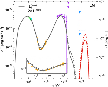
Figure 4. Leptonic model (LMBB2b) for the TXS 0506+056 flare (Ep. 1). Two SED cases (gray lines) are plotted against the observations (colored points, showing allowed ranges at 90% confidence), one with a hadronic component set to the maximum allowed proton luminosity  erg s−1 (solid gray), and the other set to twice this maximal value (dashed gray line). Corresponding all-flavor neutrino fluxes for the maximal (solid red) and “twice maximal” (dashed line) cases are also shown. Photon attenuation at
  eV due to interactions with the extragalactic background light is not included here. All-flavor neutrino-flux upper limits of producing an event similar to the IceCube-170922A are shown in blue (from Figure 4 of Aartsen et al. 2018a) for 0.5 (solid blue line) and 7.5 years (dashed blue line).
Download figure:
Standard image High-resolution imageTable 6. Parameter Values Common to All Leptonic Models (LMs) for TXS 0506+056
| B′ [G] | 0.4 |
| R′ [in cm] | 1017 |
| δ | 24.2 |
 [in erg s−1] [in erg s−1] |

|

|
1.9 |

|
3.6 |

|
1 |

|

|

|

|
Note. The isotropic-equivalent electron luminosity is  . Parameter definitions are provided in Table 5.
Download table as: ASCIITypeset image
As noted in the previous section, HE photons produced via photohadronic interactions are attenuated in the source and induce an EM cascade whose emission should emerge in the Swift-XRT and NuSTAR bands. As a result, the neutrino and proton luminosities are strongly constrained by the X-ray data. The photon spectrum obtained with  already violates the observed X-ray data points. In Figure 4, the upper limit on the all-flavor neutrino flux at the neutrino peak energy is
  .
.
In what follows, we show that our neutrino-flux limits are fairly insensitive to the exact parameter values that may affect the photomeson production optical depth.
Proton maximum energy—Motivated by the hypothesis that blazars are UHECR accelerators, i.e., at energies above  eV (Murase et al. 2012), we explore the effect of the proton maximum energy on the neutrino-flux upper limits. We thus explore cases with
  , and
, and  —see Table 7. Our results on the neutrino fluxes are presented in Figure 5.
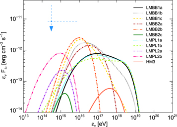
Figure 5. Upper limits on the all-flavor neutrino ( ) fluxes predicted for our modeling of the SED in the leptonic (LMx) and hadronic (HMx) models. The dashed blue line shows the value of producing an event similar to the IceCube-170922A in 7.5 years (Aartsen et al. 2018a) of data.
Download figure:
Standard image High-resolution imageTable 7. Model-specific Parameter Values for Leptonic Models (LMs) for TXS 0506+056 Discussed in the Text
| LMBB1a | LMBB1b | LMBB1c | LMBB2a | LMBB2b | LMBB2c | LMPL1a | LMPL1b | LMPL2a | LMPL2b | |
|---|---|---|---|---|---|---|---|---|---|---|
 [1044 erg s−1] [1044 erg s−1] |
0.54 | 0.27 | 0.34 | 1 | 5.4 | 10 | 0.54 | 0.54 | 10 | 10 |
| sp | 2 | 2.5 | 3 | 2 | 2 | 2 | 2 | 2 | 2 | 2 |

|
1 | 3 × 10⁶ | 3 × 10⁶ | 1 | 1 | 1 | 1 | 1 | 1 | 1 |
 [108] [108] |
30 | 30 | 30 | 1.6 | 0.16 | 0.016 | 30 | 30 | 0.016 | 0.016 |
 [erg cm−3] [erg cm−3] |
0.033 | 0.033 | 0.067 | 0.04 | 0.08 | |||||
 [K] [K] |

|
n/a | ||||||||
| α | n/a | 3 | 2 | 3 | 2 | |||||
 [keV] [keV] |
n/a | 0.05 | ||||||||
 [keV] [keV] |
n/a | 5 | ||||||||
Note. See Table 5 for parameter definitions and Table 6 for parameter values common to all LMs. In LMBB models, the external photon field is blackbody-like with comoving temperature  , while in LMPL models, it is a power law between comoving energies
  and
and  , with photon index α. In all cases,
  is the comoving energy density of the external photon field. Note that the isotropic-equivalent cosmic-ray proton luminosity is
  .
.
Download table as: ASCIITypeset image
Neutrino spectra in the LMBB1x models are more extended in energy compared to the default case (LMBB2b). They peak around 10 PeV (100 PeV) for  (
( ) for LMBB2b (LMBB2a), respectively. The number density of target photons decreases fast with increasing energy, while the photomeson production efficiency increases with energy (Murase 2017). However, the upper limits imposed on the proton luminosity and the peak neutrino flux are comparable in the LMBB2a and LMBB2b models. This is because the peak neutrino flux is bounded by the X-ray data points through EM cascades, even though the photomeson production optical depths are quite different. As such, even lower maximum proton energies, e.g.,
  , should not lead to higher upper limits on the neutrino flux. The reason is that protons with
  will produce electron–positron pairs (via the Bethe–Heitler process) on the synchrotron photons from the peak of the spectrum. Meanwhile, the photomeson interactions of the same protons on the X-ray photons (
 Hz) are less efficient (Dimitrakoudis et al. 2012). The proton luminosity cannot be arbitrarily large in this regime because the synchrotron emission from the Bethe–Heitler pairs will overshoot the X-ray data.
Proton spectral index—The slope of the power-law proton distribution is hardly constrained from the SED fitting. Here, we investigate its effects on the neutrino spectrum by considering two additional cases with  and sp = 3. For particle distributions with soft spectra (i.e.,
  ), the total energy in protons is determined by the low-energy cutoff (
 ) of the distribution. These low-energy protons, however, are of no interest for HE neutrino production. In an attempt to minimize the energy budget, while retaining the HE neutrino fluxes for
  , one has to assume
  —see Table 7. The large
  can also be justified if the proton distribution has a broken power law and the lower-energy segment has sp < 2 below the break (i.e.,
  ). Our results on the neutrino flux are presented in Figure 5 and compared to those obtained for sp = 2. The neutrino spectra become more sharply peaked as the proton distribution becomes softer, while the constraints on the 0.1–10 PeV neutrino flux approach those of our fiducial model (LMBB2b).
External radiation spectrum—Importantly, our results on the neutrino-flux upper limit are insensitive to details of the unknown photon spectrum of external radiation fields. In addition to the external blackbody spectrum, we also consider a power-law spectrum. Such a broadband spectrum might be produced, for example, by electrons accelerated with a hard spectrum in the sheath region of a structured jet, with the associated synchrotron photons—with a low synchrotron peak—serving as seeds for the EIC emission in the γ-ray range (Tavecchio et al. 2014; Tavecchio & Ghisellini 2015). From Figure 5, we see that the results for LMPL1x models with  do not differ much from those for LMBB1x models. This is because the relativistic protons at ultrahigh energies mainly interact with target photons around the synchrotron peak. On the other hand, LMPL2x models with
  give more optimistic neutrino fluxes than LMBB2c, because the photomeson interaction rate is enhanced compared to the photopair production rate (Petropoulou & Mastichiadis 2015). However, the neutrino-flux upper limits are still saturated at
  erg cm−2 s−1, similar to that for LMBB2b. We thus conclude that the neutrino-flux upper limit is
  erg cm−2 s−1 whether the unknown target spectrum of the external radiation is described by a broadband power law or a narrower blackbody. In this work, we use the blackbody spectrum as a fiducial case, which is conservative in the sense that it introduces fewer free parameters.
In summary, in the LMs (Figure 4), the γ rays are explained by the EIC emission, while there is a small contribution of the SSC component to the hard X-ray band. We note that the SSC component alone cannot explain the γ-ray component of the SED, mainly because of (i) the separation of the low- and high-energy humps of the SED, (ii) the steep Swift-XRT spectrum with the low synchrotron peak inferred by the X-shooter data, and (iii) the flat broad Fermi-LAT spectrum. Accelerated protons, generating HE neutrinos by photohadronic processes, are also present in this scenario, but with an associated EM component that is subdominant in γ rays. The maximal all-flavor neutrino flux over  is
is  erg cm−2 s−1, implying a Poisson probability to detect one event with IceCube over the six-month duration of the TXS 0506+056 γ-ray flare of at most ∼1% under our assumed conditions, which are subject to model and observational constraints but otherwise optimal for HE neutrino production. See Table 9 and Section 3.4 below for estimates of the expectation number of HE muon neutrinos for different model cases. The maximum proton isotropic-equivalent luminosity consistent with the SED is
  erg s−1. Cases with proton luminosities exceeding
  lead to higher neutrino fluxes, but they are bounded by the observed X-ray data due to EM cascade effects—as shown in the inset plot, the “twice maximal” case already violates these constraints. We studied different parameters to investigate the parameter dependence, and considered both blackbody-like and power-law spectra for the external target radiation field. As a result, we find that the LM can provide at most a few percent expectation of an associated HE neutrino detection by IceCube.
3.3. Hadronic Models (HMs)
In hadronic scenarios, while the low-energy peak in the blazar’s SED is explained by synchrotron radiation from relativistic primary electrons, the HE peak is explained by EM cascades induced by pions and muons as decay products of the photomeson production (Mannheim 1993; Mücke et al. 2003), or synchrotron radiation from relativistic protons in the ultrahigh-energy range (Aharonian 2000; Mücke et al. 2003). We coin this scenario “HM,” which stands for Hadronic Model, in reference to the hadronic origin of the γ-rays. The synchrotron and IC emission of secondary pairs may provide an important contribution to the bolometric radiation of the source. In contrast to the leptonic scenario (Section 3.2), the parameters describing the proton distribution can be directly constrained from the NuSTAR and Fermi-LAT data. For the TXS 0506+056 flare, in the hadronic scenario, the SED can be fully explained without invoking external radiation fields.
There are different combinations of parameters that can successfully explain the SED in the HM scenario (Böttcher et al. 2013; Cerruti et al. 2015). As a starting point, we search for combinations of δ and B′ that lead to rough energy equipartition between the magnetic field and protons, since the primary electron energy density is negligible in this scenario. With analytical calculations, we derive rough estimates of the parameter values for equipartition:  ,
,  G,
G,  cm, and
  GeV (Petropoulou & Dermer 2016).
The parameter values obtained by numerically modeling the SED (see Figure 6) are summarized in Table 8 and are similar to the estimates provided above. The jet power computed for this parameter set (HM1) is close to the minimum value expected in the hadronic scenarios. More specifically, the absolute power of a two-sided jet inferred for these parameters is  erg s−1, with
  erg cm−3, where
  ,
,  ,
,  are comoving energy densities of relativistic protons, electrons, and magnetic fields, respectively. As demonstrated in Figure 6, the emission from the EM cascade forms a “bridge” between the low-energy and high-energy peaks of the SED for
  (gray dotted line). Despite minimizing the power of the jet, the adopted set of parameters for HM1 cannot explain the SED due to the associated significant EM cascade component.
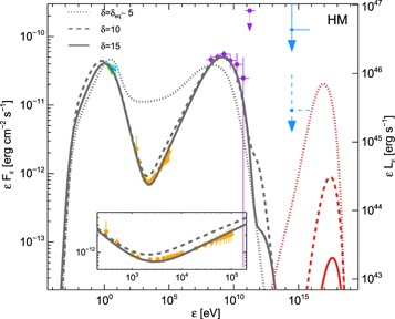
Figure 6. Hadronic model (HM3) for the SED of TXS 0506+056 flare (Ep. 1), as computed for different values of the Doppler factor (gray curves), together with resulting all-flavor neutrino fluxes (red curves) and electromagnetic observations (colored points, showing allowed ranges at 90% confidence). Photon attenuation at  eV due to interactions with the extragalactic background light is not included here. All-flavor neutrino-flux upper limits of producing an event similar to the IceCube-170922A are shown in blue (from Figure 4 of Aartsen et al. 2018a) for 0.5 (solid blue line) and 7.5 years (dashed blue line).
Download figure:
Standard image High-resolution imageTable 8. Parameter Values for Hadronic Models (HMs) for TXS 0506+056 Discussed in the Text and Presented in Figure 6
| HM1 | HM2 | HM3 | |
|---|---|---|---|
| B′ [G] | 85 | ||
| R′ [in 1016cm] | 2 | 3 | 4.5 |
| δ | 5.2 | 10 | 15 |
 [in 1043 erg s−1] 9.3 [in 1043 erg s−1] 9.3 |
0.6 | 0.06 | |

|
1.8 | ||

|
4.2 | 3.6 | 3.6 |
 [in 102] [in 102] |
6.3 | 1 | 1 |
 [in 102] [in 102] |
7.9 | 6.3 | 5 |

|
104 | ||
 [in 1046 erg s−1] [in 1046 erg s−1] |
2.7 | 0.1 | 0.01 |
| sp | 2.1 | ||

|
1 | ||

|
2 × 10⁹ | ||
Note. Parameter definitions are provided in Table 5.
Download table as: ASCIITypeset image
The EM cascade emission can be suppressed if the source becomes less opaque to the intra-source  absorption for HE photons. This can be achieved for larger values of the Doppler factor since
  (see also Murase et al. 2016; Petropoulou et al. 2017, for analytical expressions). The photon and neutrino spectra for δ = 10 and 15 are also shown in Figure 6, while the respective parameter sets (HM2 and HM3) are listed in Table 8. The SED is compatible with
  (gray solid line). However, the photomeson production optical depth becomes lower as the two-photon annihilation optical depth decreases. In fact, the sub-PeV neutrino production efficiency is related to the opaqueness for γ rays in the Fermi-LAT band (Murase et al. 2016). Furthermore, this model unavoidably leads to a higher jet power, i.e.,
  erg s−1 and
  (Petropoulou et al. 2017). Moreover, as the Doppler factor increases, the peak of the neutrino energy spectrum is pushed to the EeV energy range (Dimitrakoudis et al. 2014), while the neutrino flux in the 100 TeV–10 PeV range decreases due to the low efficiency of photomeson interactions.
HM3 demonstrates that the SED of the TXS 0506+056 flare can nicely be explained by the proton synchrotron model, but with the consequence that the HE neutrino production inside the source is very inefficient because of the X-ray constraints on EM cascade emission. The acceleration of UHECRs with  EeV is promising in this model, but cannot be reconciled with an IceCube-170922A association, since the predicted neutrino flux is too low in the 0.1–10 PeV energy range.
In summary, we find that no reconciliation of the EM and neutrino observations is possible in hadronic models (HMs; Figure 6). The proton-induced cascade model that predicts  ∼
∼  unavoidably overshoots the observed X-ray flux, giving
 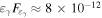 erg cm−2 s−1, which is strongly excluded. Alternatively, the proton synchrotron model can explain the TXS 0506+056 γ-ray emission, but gives a maximal neutrino flux
 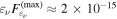 erg cm−2 s−1, which implies a very low probability for IceCube neutrino detection,
  . If the Doppler factor is sufficiently large, the proton-induced cascade emission is suppressed and can avoid overproduction of X-rays (see the main and inset plots over 0.3–100 keV), but at the price of a reduced neutrino flux; hence, only the low neutrino-flux case (red solid curve) is viable. Such low neutrino-flux cases, leading to negligible HE muon neutrino detection probabilities, cannot accommodate production of IceCube-170922A.
3.4. Implications of IceCube-170922A
Relativistic protons of energy  can interact with photons in the source and produce neutrinos with energy
  .23
The targets for photohadronic interactions can be synchrotron and IC photons emitted by primary and secondary electrons as well as external photons to the source, if present. For a typical synchrotron spectrum around the SED peak, the rectilinear approximation around the Δ resonance is usually valid (Murase & Nagataki 2006; Murase et al. 2014), and the characteristic proton Lorentz factor interacting with photons of the frequency
.23
The targets for photohadronic interactions can be synchrotron and IC photons emitted by primary and secondary electrons as well as external photons to the source, if present. For a typical synchrotron spectrum around the SED peak, the rectilinear approximation around the Δ resonance is usually valid (Murase & Nagataki 2006; Murase et al. 2014), and the characteristic proton Lorentz factor interacting with photons of the frequency  is given by (Murase 2017)

where  is the resonance energy. The respective neutrino energy, in the observer’s frame, is then given by
  . This is also an estimate of the peak energy of the HE neutrino spectrum:

Neutrinos with lower energies than  can still be produced by interactions of lower-energy protons with higher-energy photons. However, the neutrino flux at such lower energies is expected to be lower than the flux at
  due to the decreasing number density of target photons, unless the proton distribution is a super-soft power law (i.e.,
  ). Similar estimates can be derived in the presence of external radiation fields, as demonstrated in Murase et al. (2014). Note that the main target photons for the photomeson production process in the LMBB2 and LMPL2 models are photons with energies above the synchrotron peak, since even protons with
  do not satisfy the photomeson production threshold for the peak synchrotron photons—see Equation (1).
As described above, EM cascade emission induced by cosmic-ray protons readily fills the dip between the two peaks of the SED (keV to MeV energies). Thanks to the optical depth correspondence between photomeson production and two-photon annihilation, efficient production of HE neutrinos can only be achieved for conditions that lead to a stronger EM cascade emission inside the source. In particular, the proton-induced cascade model, where the Fermi-LAT γ-ray data is primarily explained by the proton-induced cascade emission itself, is strongly ruled out. Although this model naturally predicts 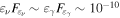 erg cm−2 s−1, which is consistent with the observation of IceCube-170922A (Aartsen et al. 2018a), the EM cascade component typically has a broadband energy spectrum that extends through the X-ray range. Thus, this model does not provide a proper description of the broadband SED. On the other hand, the proton synchrotron model can explain the blazar’s SED, but the 0.1–10 PeV neutrino flux is predicted to be very low,
  erg cm−2 s−1.
Figure 5 presents the upper limits on the all-flavor neutrino fluxes obtained in the leptonic and hadronic models for a wide set of parameters. For the maximum neutrino flux displayed in the figure,  , the corresponding muon neutrino fluence is estimated to be:

where  is the flare duration and the flavor ratio is assumed to be
 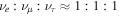 . Then, using the effective area for EHE real-time alerts,
  in the PeV range (Aartsen et al. 2017a), the expected number of muon neutrinos is estimated to be:

where the width of the neutrino spectrum is assumed to be  . We numerically confirm this analytical estimate for the different models presented in Figure 5.
Table 9 summarizes our results on the upper limits obtained for the integrated all-flavor neutrino fluxes by modeling the flaring SED of TXS 0506+056. Assuming a flare duration of ΔT = 0.5 year, we also evaluate the expected number of muon neutrinos by using the effective area for EHE real time alerts (Aartsen et al. 2017a), taking into account a correction due to the Earth attenuation toward the direction to TXS 0506+056. The exact effective area may be slightly different for IceCube-170922A (Aartsen et al. 2018a), but the results do not change within a factor of two. In the LMBB2b model or LMPL2b model, which give the most optimistic neutrino fluxes among our parameter sets, for example, the probability for IceCube to observe one event that physically originates from the TXS 0506+056 flare is evaluated to be  % based on Poisson statistics. This value is already achieved for the near-optimal case, but we allow a factor of two uncertainty for several possible reasons. First, the duration of the HE neutrino flare may be a bit longer (although the confidence of association would be reduced for longer durations). Second, the EHE effective area for IceCube-170922A may be slightly different. Then, taking into account these variations as well as model uncertainties, we may regard the case for the proton luminosity of
  as the most conservative limit, which gives
  %.
%.
Table 9.
The Upper Limit on the All-flavor Neutrino Flux  for the Different Models that Satisfactorily Explain the Flaring SED of TXS 0506+056—for Details, See Sections 3.2 and 3.3
 [erg cm−2 s−1] [erg cm−2 s−1] |

|
||
|---|---|---|---|
| 100 TeV–1 PeV | 100 TeV–10 PeV | ≤10 PeV | |
| LMBB1a | 1.6 × 10⁻¹⁴ | 4.5 × 10⁻¹³ | 1 × 10⁻³ |
| LMBB1b | 5.2 × 10⁻¹⁴ | 1.7 × 10⁻¹² | 4 × 10⁻³ |
| LMBB1c | 9.1 × 10⁻¹⁴ | 2.7 × 10⁻¹² | 6 × 10⁻³ |
| LMBB2a | 4.5 × 10⁻¹⁴ | 1.1 × 10⁻¹² | 3 × 10⁻³ |
| LMBB2b | 1.8 × 10⁻¹³ | 3.6 × 10⁻¹² | 8 × 10⁻³ |
| LMBB2c | 2.5 × 10⁻¹⁴ | 7.3 × 10⁻¹⁴ | 2 × 10⁻⁴ |
| LMPL1a | 3.1 × 10⁻¹⁴ | 5.2 × 10⁻¹³ | 1 × 10⁻³ |
| LMPL1b | 9 × 10⁻¹⁴ | 6.3 × 10⁻¹³ | 1 × 10⁻³ |
| LMPL2a | 2.5 × 10⁻¹³ | 5.2 × 10⁻¹³ | 5 × 10⁻³ |
| LMPL2b | 1.2 × 10⁻¹² | 2 × 10⁻¹² | 1 × 10⁻² |
| HM3 | 1.6 × 10⁻¹⁶ | 2 × 10⁻¹⁵ | 4 × 10⁻⁶ |
Note. The reported values correspond to the neutrino fluxes integrated over 0.1–1 PeV and 0.1–10 PeV ranges. The last column shows the expected number of muon neutrinos below 10 PeV for a flare duration ΔT = 0.5 year.
Download table as: ASCIITypeset image
4. Discussion
The contribution of blazar jets to the diffuse neutrino flux has been calculated based on both leptonic and hadronic scenarios for the observed γ-rays, under the common assumption of a constant neutrino flux (Murase et al. 2014; Tavecchio et al. 2014; Padovani et al. 2015; Tavecchio & Ghisellini 2015; Rodrigues et al. 2018). Most of the most optimistic scenarios for the diffuse neutrino emission from blazars (for a review, see Murase 2017) can now be constrained by IceCube (e.g., Aartsen et al. 2016a, 2016b, 2017b). In addition, all of the model-independent analyses (stacking, multiplet, and auto-correlation analyses) have disfavored the blazar population as the dominant (∼100%) origin of IceCube’s neutrinos, implying that their contribution is less than ∼3%–30% of the diffuse neutrino intensity in the 0.1–1 PeV range (Aartsen et al. 2015, 2017b, 2017c; Murase & Waxman 2016). Importantly, even if the blazar contribution to the diffuse neutrino flux is subdominant, the flaring blazar-associated neutrinos are detectable with the current detector since the atmospheric backgrounds can be reduced by temporal and spatial coincidence. Although blazars do not exhibit the extreme variability of nonrepeating transients like gamma-ray bursts and supernovae, they are highly variable on different timescales and across the EM spectrum (Kataoka et al. 2001; Abdo et al. 2010; González-Martín & Vaughan 2012; Sobolewska et al. 2014), and have long been one of the most promising possibilities for HE neutrino production (Atoyan & Dermer 2001; Dermer et al. 2012, 2014; Halzen & Kheirandish 2016; Kadler et al. 2016; Petropoulou et al. 2016; Turley et al. 2016; Gao et al. 2017).
We presented the time-averaged data for Ep. 1 and Ep. 2 and used the former for multimessenger modeling of the source SED. Although we have argued that this is a reasonable approach, it has some limitations. In particular, we cannot exclude the possibility that physical conditions of the source change drastically on a short timescales. Although there is currently no evidence of such rapid variability, this could affect the results of our time-average SED modeling. Nevertheless, the EM cascade effects are inevitable and the resulting X-ray component must appear. We thus expect that our conclusions are robust, since the upper limits on neutrino fluence are basically set by the observed X-ray fluence.
We modeled the SED for Ep. 1 with a 30 day window. The X-ray flux varies by a factor of 6 within 60 days, but the time-average SED for Ep. 2 does not differ much from that for Ep. 1. This indicates that the physical conditions are approximately similar during Ep. 1 and Ep. 2, which justifies the setup of our calculations. The flare duration that is relevant for estimates of the signal neutrino fluence is at least  days and the γ-ray data suggest that a duration of
  is possible.
As noted above, it is the neutrino fluence (i.e., the product of the duration of neutrino emission and the neutrino flux) that matters in the calculation of the expected number of events. It is therefore likely that the expected number of events from a nonflaring blazar integrated over the IceCube lifetime is larger than the one expected from a flare. In our optimal case, if the SED shape and X-ray flux in the steady state remain similar to those in the flaring state, the expectation value of the number of muons that can be found in the eight-year point-source analysis on upgoing muons is ∼1 event. Thus, time-averaged X-ray fluxes had to be higher in the past to obtain ∼13 neutrino events (Aartsen et al. 2018b). To properly address this question, one would need to have a good description of the nonflaring SED of the source, especially in the X-ray range. We plan to compare the flaring emission with the nonflaring emission of TXS 0506+056 in a dedicated future work (M. Petropoulou et al. 2018 in preparation).
Although our results on the neutrino-flux upper limit in the LMs are insensitive to details of the external photon field, we briefly discuss possible origins of the external photons. The typical photon energy of the external radiation field in the black hole rest frame is  eV and its energy density is
  erg cm−3 (see Table 7). The putative external photon field is compatible with scattered disk emission or soft emission from the sheath region of the blazar jet (Dermer et al. 2014; Tavecchio & Ghisellini 2015). Any additional external component should not exceed the observed fluxes in the optical, UV, and X-ray data. Thus, its luminosity should be
  erg s−1, depending on the spectral shape.
In the scattered disk emission case, if there is a scattering region with the Thomson optical depth  at radius R, the energy density of the scattered emission can be
  erg cm−3. Alternatively, dissipation in the sheath region of the jet may lead to electron acceleration and associated synchrotron emission with a peak energy of
  eV and luminosity of
  , where
  is the Lorentz factor of the sheath region.
Third, external photons can be provided by the possible broadline region, and the energy density of the broadline region can be written as  erg cm−3, where
  is the covering fraction (Ghisellini & Tavecchio 2008). However, there are two drawbacks. The lack of broadline signatures in the optical spectrum of TXS 0506+056 and other BL Lac objects suggests that such line emissions are weak.
Also, such emissions will only be important when the blob is located in the broadline region. If we follow the treatment in Murase et al. (2014), the observed γ-ray luminosity indicates that the broadline region is located at  cm, so that the typical emission radius would be larger than the radius of the possible broadline region.
Even though blazars like TXS 0506+056 could make a significant contribution to the diffuse neutrino flux, it is premature to extrapolate our findings from the modeling of the TXS 0506+056 flare to other blazars. A more dedicated study is left for future work, after a representative set of flares have been modeled individually (see also Padovani et al. 2015). So far, the only other flare that was modeled with the same numerical code is the 13-day (2010) flare of the high-frequency peaked blazar Mrk 421 (Petropoulou et al. 2016). In that case, the available EM data could be explained with a higher neutrino-to-γ-ray luminosity ratio than we find here. If we were to take the neutrino-to-γ-ray luminosity ratio for the TXS 0506+056 flare as representative of flaring blazars, their contribution to the diffuse neutrino flux would be smaller than previous estimates.
Finally, as we emphasized, our theoretical interpretation is based on the single-zone model. In this assumption, the broadband EM and HE neutrino emissions are produced in the same localized region in the blazar jet. Efficient HE neutrino production requires large optical depths for photomeson production. This, in turn, implies that the emitting region is optically thick for HE γ-rays (Murase et al. 2016). This is especially the case for blazars that have soft photon spectra, in which the EM energy of the attenuated very HE photons will reappear at lower energies through an EM cascade. The tight constraints stemming from the large optical depth of a localized region could be alleviated, if the photon and neutrino emissions originate from different regions in the jet, as in multizone models (Dermer et al. 2012, 2014; Murase et al. 2014). Although a detailed discussion must be deferred to future work (Murase et al. 2018), the constraints from the EM cascade are unavoidable even for such multizone models, so that further ad hoc adjustments of the source parameters seem necessary.
5. Conclusions
We have used the best available multiwavelength data to construct the broadband SED of TXS 0506+056, over 10 orders of magnitude in photon energy from ≈1 eV to >10 GeV, proximate to its likely (∼3σ; Aartsen et al. 2018a) emission of the high-energy neutrino IceCube-170922A. Working with this SED and the likely neutrino association, we have explored multimessenger models for TXS 0506+056 to evaluate whether this neutrino association is physically reasonable, and if so, under what conditions of the blazar jet and jet environment.
We find that a leptonic scenario with a radiatively subdominant hadronic component provides the only physically consistent single-zone picture for this source’s multimessenger (EM and neutrino) emissions. If IceCube-170922A is associated with this flaring blazar, then physical conditions were close to optimal for neutrino production during its flare. We find a maximal all-flavor neutrino flux over  of
of  erg cm−2 s−1. The inferred ratio of proton to electron luminosities is large,
  –500, with smaller values prohibited because increased optical depth to
  would suppress the observed γ-rays.
Under these conditions, we find a probability of  to 2% for IceCube to detect an HE muon neutrino in real time at some point during the blazar’s six-month flare.
Since the blazar’s >GeV emissions are dominated by leptonic processes, and since EM cascades efficiently redistribute hadronic EM emissions across the spectrum, we find that the SED exhibits its greatest sensitivity to hadronic acceleration processes across its 0.1–100 keV “dip.” Flux variations over this energy range are more likely to reflect the source’s high-energy neutrino emissions than its GeV–TeV flux state. We thus find that, going forward, regular X-ray monitoring of TXS 0506+056 and related blazars, in conjunction with continued monitoring by high-energy neutrino observatories, will provide a critical test of single-zone blazar models. Moreover, careful selection of temporal acceptance windows via X-ray observations, as in Turley et al. (2016), will likely yield the most sensitive search for further multimessenger sources.
Finally, we find that under the observed flaring conditions, assuming the IceCube-170922A association holds, TXS 0506+056 was not a significant UHECR accelerator. This is because a proton spectrum extending to  ≳ 3 EeV would yield a neutrino spectrum peaking above 100 PeV (Murase et al. 2014); with the neutrino peak flux bounded by X-ray observations via cascade effects, this would strongly suppress the 0.1–10 PeV neutrino flux (Figure 5).
It is possible that multizone models, which more readily decouple blazar EM and neutrino emissions, may ultimately be required to explain multimessenger observations of TXS 0506+056 and other blazars. Independent of whether this particular source association holds, our results demonstrate that the detection of even one or two coincident neutrinos can grant us deep insight into a source, and should energize future searches for further multimessenger sources.
We note that the neutrino upper flux data points in Figures 4–6 have been added after the completion of the modeling using data points from Aartsen et al. (2018a).
The authors thank the referee for valuable comments that helped to improve the manuscript. The authors thank the IceCube Collaboration for publicly distributing HE neutrinos in real-time, the Swift and NuSTAR teams for their rapid responses to our target of opportunity requests, and the Fermi collaboration for their publicly available data and analysis software. The authors acknowledge helpful discussions with L. Hagen, J. Charlton, and M. Eracleous. A.K., D.B.F., J.J.D., and C.F.T. acknowledge support from the National Science Foundation under grant PHY-1412633; A.K. acknowledges support from the National Aeronautics and Space Administration Swift Guest Investigator Program under grant NNX17AI95G. The work of K.M. is supported by NSF Grant No. PHY-1620777 and the Alfred P. Sloan Foundation. A.K. and K.M. gratefully acknowledge support from the Institute for Gravitation and the Cosmos at the Pennsylvania State University. J.K. and A.T. acknowledge support from NASA contract NAS5-00136. P.A.E. and J.P.O. acknowledge support from the UK Space Agency. M.P. acknowledges support from the L. Jr. Spitzer Postdoctoral Fellowship. S.C. thanks the Centre National d’Etudes Spatiales (CNES) for support and funding. Based on observations collected at the European Organization for Astronomical Research in the Southern Hemisphere under ESO program 099.D-0640(A).
Correspondence regarding this work should be sent to Kohta Murase () or Maria Petropoulou () for theoretical interpretations, and Azadeh Keivani () or Derek Fox () for observations.
Software: XSPEC (Arnaud 1996), HEAsoft (v6.22.1), X-shooter pipeline (v.2.9.3; Goldoni et al. 2006; Modigliani et al. 2010), Reflex (Freudling et al. 2013), Molecfit (Kausch et al. 2015; Smette et al. 2015), Fermi Science Tools (https://fermi.gsfc.nasa.gov/ssc/data/analysis/software/), SOPHIA (Mücke et al. 2000).
Footnotes
- 18
AMON website: https://www.amon.psu.edu/.
- 19
NASA/IPAC Infrared Science Archive: https://irsa.ipac.caltech.edu/.
- 20
UVOT Calibrations Database (CALDB): https://heasarc.gsfc.nasa.gov/docs/heasarc/caldb/data/swift/uvota/index.html.
- 21
Fermi Science Tools can be downloaded from https://fermi.gsfc.nasa.gov/ssc/data/analysis/software/.
- 22
We will refer to this scenario simply as hadronic for simplicity.
- 23
Hadronuclear reactions such as proton–proton collisions in blazar jets are expected to be too inefficient compared to the photomeson production process, for typical values of the jets’ plasma density (Atoyan & Dermer 2003; Murase et al. 2014). Also, even ad hoc high-density environments are similarly (∼order of magnitude) constrained by the cascade bound.