Abstract
We present the discovery that ASASSN-14ko is a periodically flaring active galactic nucleus at the center of the galaxy ESO 253-G003. At the time of its discovery by the All-Sky Automated Survey for Supernovae (ASAS-SN), it was classified as a supernova close to the nucleus. The subsequent 6 yr of V- and g-band ASAS-SN observations revealed that ASASSN-14ko has nuclear flares occurring at regular intervals. The 17 observed outbursts show evidence of a decreasing period over time, with a mean period of P0 = 114.2 ± 0.4 days and a period derivative of  . The most recent outburst in 2020 May, which took place as predicted, exhibited spectroscopic changes during the rise and had a UV bright, blackbody spectral energy distribution similar to tidal disruption events (TDEs). The X-ray flux decreased by a factor of 4 at the beginning of the outburst and then returned to its quiescent flux after ∼8 days. The Transiting Exoplanet Survey Satellite observed an outburst during Sectors 4–6, revealing a rise time of 5.60 ± 0.05 days in the optical and a decline that is best fit with an exponential model. We discuss several possible scenarios to explain ASASSN-14ko’s periodic outbursts, but currently favor a repeated partial TDE. The next outbursts should peak in the optical on UT 2020 September 7.4±1.1 and UT 2020 December 26.5±1.4.
1. Introduction
There are numerous physical processes that lead to variability in the nuclei of galaxies. Every massive galaxy likely houses a supermassive black hole (SMBH; Kormendy & Richstone 1995; Kormendy & Ho 2013), and the past several decades have been spent unraveling their accretion and variability processes (for reviews, see, e.g., Ulrich et al. 1997; Ho 2008; Heckman & Best 2014; Yuan & Narayan 2014; Padovani et al. 2017; Hickox & Alexander 2018; Komossa 2018; Blandford et al. 2019). Without the ability to spatially resolve the immediate vicinity of the SMBH, other methods must be used to probe accretion physics.
Variable accretion in active galactic nuclei (AGNs) is the primary driver of nuclear variability. Most quasars appear to vary in brightness stochastically with statistical properties that can be modeled relatively well by a damped random walk (DRW; e.g., Kelly et al. 2008; Kozłowski et al. 2010; MacLeod et al. 2010; Zu et al. 2013). Signatures that deviate from DRW behavior, namely, periodic or semi-periodic features, have been suggested as possible indicators for a binary system at the galaxy’s core (e.g., Komossa 2006).
This has led to searches for periodic signals in AGN light curves to identify SMBH binaries. For example, Graham et al. (2015a) used the Catalina Real-time Transient Survey (CRTS) to search for sub-parsec SMBH binaries. They reported 111 candidates that showed evidence of periodicity associated with a Keplerian orbit. Another study by Charisi et al. (2016) used the Palomar Transient Factory to identify 33 candidates with evidence for periodic variability. Liu et al. (2015, 2016, 2019) searched for periodicity in Pan-STARRS1’s Medium Deep Survey, ultimately finding one candidate, PSO J185. Other candidates with quasi-periodic/periodic variability include NGC 4151 with an estimated period of ∼16 yr (e.g., Oknyanskij 1978; Pacholczyk et al. 1983; Guo et al. 2006; Oknyanskij & Lyuty 2007; Bon et al. 2012), and PG 1302-102 with an estimated period of 1884 days (Graham et al. 2015b) or 1899 days (Kovačević et al. 2019). Simulations have shown that periodic variability is expected in the light curves of SMBH binaries at sub-parsec separations due to a variety of processes, including modulated mass accretion onto the binary (e.g., D’Orazio et al. 2013; Farris et al. 2014; Gold et al. 2014) or relativistic Doppler boosting of the minidisks formed as a result of the binary interaction (D’Orazio et al. 2015).
Aside from low-level variability, AGNs can also show outbursts or flares in which the brightness of the AGNs increases dramatically for a short period of time before returning to a level of relative quiescence. The best example of quasi-periodic optical flares is the 12 yr outburst cycle of OJ 287. These were first reported by Sillanpaa et al. (1988), who suggested that outbursts are due to perturbations of the primary black hole’s accretion disk during pericenter passages of the secondary black hole on a 12 yr orbital cycle. Relativistic effects like precession probably alter the orbital geometry so that the events are not strictly periodic (see, Valtonen et al. 2006; Laine et al. 2020). The most recent flare detected from OJ 287 brightened in the X-ray, UV, and optical, and occurred between 2020 April and June, which was consistent with the predictions of the binary black hole model (Komossa et al. 2020). Another candidate is IC 3599, which has competing theories for the cause of its X-ray/optical flares. Grupe et al. (2015) proposed accretion disk instabilities as the cause of the recurring ∼9.5 yr flares, while Campana et al. (2015) argued for partial tidal disruption events (TDEs).
TDEs also lead to variable SMBH activity. In a TDE, a star is torn apart when it passes within the tidal radius of the SMBH at the center of its host galaxy, as the tidal shear forces overwhelm the self-gravity of the star. The disrupted stellar material subsequently produces a luminous transient flare of electromagnetic radiation that we observe as a TDE. Total disruptions from parabolic orbits (Hills 1975; Rees 1988; Evans & Kochanek 1989; Phinney 1989) lead to half of the disrupted star’s mass being ejected, while the other half is gravitationally bound and asymptotically returns to pericenter at a fallback rate proportional to t−5/3.
In the case of a partial TDE, the star survives the encounter with the SMBH and only a fraction of the stellar material is tidally stripped, leaving the stellar core intact. Guillochon & Ramirez-Ruiz (2013) found that the fallback rate for partial TDEs at late times becomes steeper than t−5/3 because there is less debris with orbital binding energies close to zero if the stellar core survives the encounter. Coughlin & Nixon (2019) found a fallback rate proportional to t−9/4, which is effectively independent of the mass of the core that survives the passage close to the black hole. This fallback rate is supported by the hydrodynamical simulations of Miles et al. (2020). Hydrodynamical simulations also indicate that partial disruptions can repeat, causing episodic mass transfer from the star to the SMBH at every pericenter passage, resulting in a series of low-level flares that repeat on the orbital timescale (MacLeod et al. 2013). Partial disruptions are most easily achieved for giant stars (e.g., Guillochon & Ramirez-Ruiz 2013; MacLeod et al. 2013), which might also be created as stellar merger products (e.g., Antonini et al. 2011; MacLeod et al. 2012). In addition, circular extreme mass ratio inspirals (EMRIs) can result in repeated mass transfers that power quasi-periodic sequences of SMBH accretion-powered flares (Metzger & Stone 2017).
Most theoretical predictions for TDEs predate any observations of the phenomenon. The first observational claims of TDEs were soft X-ray outbursts from otherwise quiescent galaxies (e.g., Bade et al. 1996; Grupe et al. 1999; Komossa & Greiner 1999; Greiner et al. 2000; Gezari et al. 2003; Komossa 2015). Since then, TDE flares have been discovered at a range of wavelengths, including the hard X-ray (e.g., Bloom et al. 2011; Burrows et al. 2011; Cenko et al. 2012a; Pasham et al. 2015), soft X-ray (e.g., Komossa & Bade 1999; Donley et al. 2002; Maksym et al. 2010; Saxton et al. 2012), ultraviolet (e.g., Stern et al. 2004; Gezari et al. 2006, 2008, 2009), and optical (e.g., van Velzen et al. 2011; Cenko et al. 2012b; Gezari et al. 2012; Arcavi et al. 2014; Holoien et al. 2014b, 2016a, 2016b, 2018, 2019b, 2019a, 2020; Vinkó et al. 2015; van Velzen et al. 2021; Hinkle et al. 2021). Due to the intrinsic multiwavelength properties of both TDEs and AGNs, one problem is to identify characteristics that clearly distinguish between the two objects, notably using X-rays (Auchettl et al. 2018). This is becoming more important with the discoveries of more ambiguous transients such as ASASSN-18el (Trakhtenbrot et al. 2019; Ricci et al. 2020) and ASASSN-18jd (Neustadt et al. 2020).
Here we report the discovery and long-term observation of a series of periodic outbursts from ASASSN-14ko, which is associated with the AGN ESO 253-G003 (z = 0.042489, Aguero et al. 1996). ESO 253-G003 was spectroscopically classified as a Type 2 Seyfert by Lauberts (1982). In Section 2, we discuss the discovery of ASASSN-14ko and the photometric and spectroscopic data used in this analysis. In Section 3, we discuss the host properties, and in Section 4, we discuss the light curve and the periodic nature of the outbursts. The spectroscopic results are presented in Section 5, and we discuss several theoretical interpretations of these periodic flares in Section 6. Throughout this paper, we assume a flat Ωm
= 0.3 universe, corresponding to a luminosity distance of ≈188 Mpc and a projected scale of  . We also assume a Galactic extinction of AV = 0.118 mag (Schlafly & Finkbeiner 2011).
2. Discovery and Observations
On 2014 November at 14.28 UT, the All-Sky Automated Survey for SuperNovae (ASAS-SN; Shappee et al. 2014; Kochanek et al. 2017) triggered on a nuclear transient associated with ESO 253-G003 at V ∼ 17.0 mag and reported it as ASASSN-14ko (Holoien et al. 2014a, 2017). We will refer to this object as ASASSN-14ko throughout this paper. As reported in Holoien et al. (2014a), a follow-up spectrum on 2014 November 16 using the Boller and Chivens (B&C; Osip et al. 2004) spectrograph on the du Pont 2.5 m Telescope at Las Campanas Observatory revealed a strong blue continuum and the emission lines were consistent with a Type 2 Seyfert. At the time, the event was considered to be a Type IIn supernova (SN) with a blue continuum projected very close to the nucleus of a Type 2 Seyfert, but strong AGN activity was not ruled out as a possibility (Holoien et al. 2014a).
UltraViolet/Optical Telescope (UVOT) and X-Ray Telescope (XRT) observations by the Neil Gehrels Swift Observatory (Swift hereafter, Gehrels et al. 2004) were taken on UT 2014 November 16, 19, 21, 23, and 27 (PI: T. W.-S. Holoien, ToO ID: 33529). These observations showed that the central region of the galaxy had significantly brightened in the UV but were consistent with archival magnitudes in the optical. These Swift data also revealed X-ray emission, with fluxes of (2.85 ± 0.8) × 10−13 and (3.1 ± 0.7) × 10−13 erg cm−2 s−1 on 2014 November 16 and 19, respectively. The X-ray spectrum was consistent with highly absorbed AGNs with a column density of ∼1023 cm−2 and a luminosity of LX ∼ 3 × 1042 erg s−1 (Holoien et al. 2014a).
As part of ongoing work to examine the long-term behavior of AGNs observed by ASAS-SN, a full light curve of ESO 253-G003 was extracted in 2020 February. The complete V- and g-band light curve through 2020 September is shown in Figure 1. Visual examination of the light curve revealed 16 roughly equal amplitude flares evenly spaced out over 6 yr, as shown in Figure 2. The 17 outburst in Figure 2 was then predicted and observed. The original ASASSN-14ko trigger corresponds to the second outburst in the series. This initiated the further analysis and photometric and spectroscopic follow-up of ASASSN-14ko, which we report here. All photometric data used in this analysis are presented in Table 1.
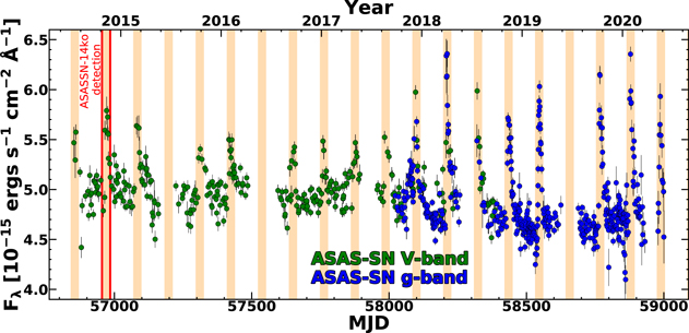
Figure 1. The complete ASAS-SN V-band (green) and g-band (blue) data for ESO 253-G003. Seventeen complete flares were detected between 2014 and 2020. The expected flare peaks predicted by the model described in Section 4.1 are shown by the shaded regions with widths of 30 days.
Download figure:
Standard image High-resolution image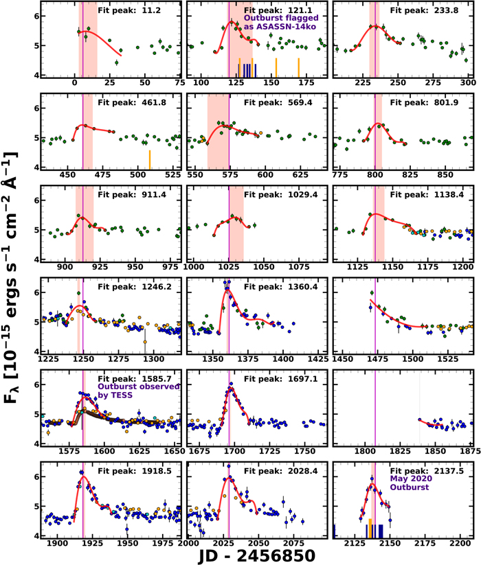
Figure 2. Light curves of ASASSN-14ko spanning 2014–2020 and demonstrating its periodic flaring behavior. The ASAS-SN V-band and g-band data are shown in green and blue, respectively. The three Transiting Exoplanet Survey Satellite (TESS) sector observations are included in light red. Asteroid Terrestrial impact Last Alert System (ATLAS) o-band data are shown in orange and ATLAS c-band data are shown in cyan. Swift epochs are denoted by dark blue marks, and spectral epochs are shown by orange marks at the bottom of each panel. The fifth-order polynomial fits for each outburst are shown in red along with red-shaded regions corresponding to estimates for each peak time and its uncertainty. The magenta vertical lines show the predicted peaks for the model with a period derivative described in Section 4.1.
Download figure:
Standard image High-resolution imageTable 1. Photometry of ASASSN-14ko Used in This Analysis
| JD | Band | Fλ (10−15 erg s−1 cm−2 Å−1) | Fλ Error (10−15 erg s−1 cm−2 Å−1) |
|---|---|---|---|
| 2458957.425 | X-ray | 0.18 | 0.03 |
| 2458957.428 | W2 | 6.76 | 0.25 |
| 2458957.431 | M2 | 4.68 | 0.17 |
| 2458957.425 | W1 | 4.16 | 0.15 |
| 2458957.427 | U | 3.61 | 0.13 |
| 2458952.424 | B | 4.28 | 0.08 |
| 2458022.900 | g | 4.94 | 0.11 |
| 2456790.495 | V | 4.94 | 0.13 |
| 2457453.755 | c | 0.14 | 0.02 |
| 2458008.130 | o | 0.21 | 0.01 |
| 2458411.544 | ITESS | 0.02 | 0.01 |
| 2458958.385 | r | 4.02 | 0.04 |
Note. Only the first observation in each band is shown here to demonstrate its form and content. The X-ray data are on a scale of 10−12 erg s−1 cm−2.
Only a portion of this table is shown here to demonstrate its form and content. A machine-readable version of the full table is available.
Download table as: DataTypeset image
2.1. ASAS-SN Photometry
ASAS-SN is a network of 20 robotic telescopes hosted by the Las Cumbres Observatory Global Telescope (LCOGT: Brown et al. 2013) at five sites around the globe. Each telescope consists of four 14 cm aperture Nikon telephoto lenses with 8.0″ pixels and a 4.5° × 4.5° field of view. ASAS-SN’s primary objective is to discover supernovae (SNe) by surveying the entire visible sky every night. The ASAS-SN data shown in Figure 2 includes both V-band and g-band observations. In 2018, the first two ASAS-SN mounts transitioned from the V band to g band to match the three ASAS-SN telescopes deployed in 2017–2018.
The data were reduced using a fully automated pipeline based on the ISIS image subtraction package (Alard & Lupton 1998; Alard 2000). Each photometric epoch (usually) combines three dithered 90 s image exposures with a 4.47° × 4.47° field of view that is subtracted from a reference image. We then used the Image Reduction and Analysis Facility (IRAF) package apphot (Tody 1986, 1993) to perform aperture photometry with a 2 pixel, or approximately 16.0″, radius aperture on each subtracted image, generating a differential light curve. The photometry was calibrated using the American Association of Variable Star Observers (AAVSO) Photometric All-Sky Survey (Henden et al. 2015). All low-quality ASAS-SN images of ESO 253-G003 were inspected by eye, and images with clouds or other systematic problems were removed.
2.2. Swift UVOT Photometry
Following the original discovery, we requested Swift UVOT (Roming et al. 2005) ToO observations (ToO ID: 33529). Then, after we discovered its periodic nature, we again requested Swift data (ToO IDs: 13836, 13979, 14005) to monitor ASASSN-14ko during quiescence and then during the outburst predicted for UT 2020 May 18.5 (see below). Data were obtained in six filters (Poole et al. 2008): V (5468 Å), B (4392 Å), U (3465 Å), UVW1 (2600 Å), UVM2 (2246 Å), and UVW2 (1928 Å). We used the HEAsoft (HEASARC 2014) software task uvotsource to extract the source counts using a 16.0″ radius aperture and used a sky region of ∼40,0″ radius to estimate and subtract the sky background. This aperture size was chosen to match the ASAS-SN photometry. All fluxes were aperture corrected and converted into magnitudes and fluxes using the most recent UVOT calibration (Poole et al. 2008; Breeveld et al. 2010). The UVOT transient, host, and calibration star magnitudes were corrected for Galactic extinction. In order to measure only the transient flux in each epoch, the quiescent host fluxes were subtracted in the same aperture. The host magnitudes are given in Table 2. We converted the Swift UVOT B and V magnitudes to Johnson B and V magnitudes using the standard color corrections. 25
Table 2. Host Magnitudes of ESO 253-G003 Measured Using a 16.0″ Aperture
| Filter | Magnitude | Uncertainty |
|---|---|---|
| UVW2 | 16.56 | 0.02 |
| UVM2 | 16.58 | 0.02 |
| UVW1 | 16.43 | 0.02 |
| U | 15.95 | 0.02 |
| B | 15.26 | 0.01 |
| g | 15.00 | 0.01 |
| V | 14.77 | 0.01 |
| r | 14.46 | 0.01 |
| R | 14.48 | 0.01 |
| i | 14.23 | 0.01 |
| J | 13.45 | 0.04 |
| H | 12.65 | 0.05 |
| Ks | 11.76 | 0.04 |
| W1 | 12.78 | 0.02 |
| W2 | 12.24 | 0.02 |
| W3 | 10.40 | 0.02 |
| W4 | 9.11 | 0.02 |
Note. The UVW2-, UVM2-, UVW1- and U-band magnitudes were determined from Swift data taken in 2020 April during pre-outburst quiescence. Johnson–Cousins BVR and SDSS gri magnitudes were determined from LCOGT, Swift B and V, and amateur astronomer data also taken in 2020 April. The magnitudes were combined by averaging the data weighted by the inverse squares of the uncertainties. All magnitudes are in the AB system.
Download table as: ASCIITypeset image
There are three additional observations of this galaxy in the Swift data archive under the identification SWIFT J0525.3-600 (Obs ID: 37354, PI: C.B. Markwardt). These observations were obtained to investigate the Swift Burst Alert Telescope (BAT) source reported by Baumgartner et al. (2013) in their 70 month catalog and identified with the nearby blazar PKS 0524-460. However, Lansbury et al. (2017) concluded that ESO 253-G003 was in fact the BAT source rather than PKS 0524-460. The three Swift epochs are consistent with the quiescent magnitudes we measure from the later data and there were too few observations to usefully add to the constraints on the times of the outbursts.
2.3. ATLAS Photometry
The ATLAS survey (Tonry et al. 2018) consists of two 0.5 m f/2 Wright Schmidt telescopes on Haleakalā and at the Mauna Loa Observatory. Designed primarily for detecting hazardous asteroids, the telescopes obtain four 30 s exposures of 200–250 fields per night. This corresponds to roughly a quarter of the visible sky. ATLAS uses two broadband filters, the “cyan” (c) filter covering 420–650 nm and the “orange” (o) filter covering 560–820 nm (Tonry et al. 2018).
The ATLAS pipeline performs flat-field corrections for each image as well as astrometric and photometric calibrations. Reference images of the host galaxy were created by stacking multiple images taken under ideal conditions and this reference was then subtracted from each ATLAS epoch to isolate the flux from the transient. We performed forced photometry on the subtracted ATLAS images of ASASSN-14ko as described in Tonry et al. (2018). ATLAS images taken on the same night were stacked. The resulting ATLAS o- and c-band photometry and 3σ limits are included also in Figure 2.
2.4. TESS Photometry
ASASSN-14ko was observed by the TESS (Ricker et al. 2014) during Sectors 4–6, which occurred between 2018 October 18 and 2019 January 7. Similar to the process applied to the ASAS-SN data, we used the ISIS package (Alard & Lupton 1998; Alard 2000) to perform image subtraction on the 30 minute cadence TESS full-frame images (FFIs) to obtain high fidelity light curves of this galaxy. This process is fully described in Vallely et al. (2019).
We construct independent reference images for each sector as opposed to utilizing a single reference image over all sectors to avoid introducing problems created by the field rotations between sectors. The reference images were built using the first 100 good-quality FFIs for each sector. FFIs were considered poor-quality if the sky background levels or point-spread function (PSF) widths were above average for the sector. FFIs were also excluded from our analysis if they had data quality flags, or were taken when the spacecraft’s pointing was compromised due to instrument anomalies, or when scattered light affected the images.
The measured fluxes were converted into TESS-band magnitudes using an instrumental zero-point of 20.44 electrons per second from the TESS Instrument Handbook (Vanderspek et al. 2018). TESS observes in a single broadband filter, spanning roughly 6000–10000 Å with an effective wavelength of ∼7500 Å, and TESS magnitudes are calibrated to the Vega system (Sullivan et al. 2015). The TESS light curve is also shown in Figure 2.
2.5. LCOGT Photometry
We obtained photometric observations from the LCOGT (Brown et al. 2013). The B-, V-,  -,
-,  -, and
  -band observations were taken using the 1 m telescope at Siding Spring Observatory in New South Wales, Australia. The LCOGT photometric observations began on 2020 April 13 in quiescence and continued through the midpoint of the 2020 May outburst when telescope horizon observing limits prevented further observations. Aperture magnitudes were obtained using a 16.0″ radius aperture using the IRAF apphot package using an annulus to estimate and subtract background counts. We used stars with the AAVSO Photometric All-Sky Survey (APASS) DR 10 magnitudes to calibrate the data. Similar to the process for the UVOT observations, the aperture magnitudes were corrected for Galactic extinction. The host galaxy flux was measured using the 2020 April quiescent data and subtracted to isolate the flux from the transient.
2.6. Amateur Astronomer Photometry
Amateur astronomers at four different observatories observed ASASSN-14ko starting shortly after it was discovered to be periodically flaring. Data were taken at the Moondyne Observatory, east of Perth, Australia, using a 0.4 m telescope with AOX adaptive optics between 2020 April 28 and June 8 and on a daily cadence between 2020 May 10 and 28. BC -, V-, GS -, RS -, and IC -band images were obtained with guided 120 s exposures. The data were reduced and calibrated with standard procedures, and then stacked with three and five image sets aligned using background stars. Data were also collected using a 41 cm telescope at Savannah Skies Observatory from Queensland, Australia. The bias and dark subtracted data were taken in the B, V, RC , and IC bands using 180 s exposures. ASASSN-14ko was observed from Bronberg Observatory in South Africa using 14- and 12-inch telescopes in the R band with 15 s exposures. The images were calibrated and then sets of eight images were stacked per night. Finally, ASASSN-14ko was observed from Dogsheaven Observatory in Brazil using the B, V, RC , and IC filters. The images were observed with 120 s exposures using a 14-inch telescope and calibrated.
All these images were then astrometrically calibrated and aperture magnitudes were measured using the IRAF apphot package and a 16.0″ aperture following the same procedures described for the Swift UVOT and LCOGT data.
2.7. Spectroscopic Observations
The first available observation of ESO 253-G003 was obtained by Kewley et al. (2001) on 1996 February 19. At that time, ESO 253-G003 was classified as a Seyfert 2 galaxy. When ASASSN-14ko was first discovered, we took a follow-up spectrum using the B&C spectrograph on the du Pont 2.5 m Telescope at Las Campanas Observatory on 2014 November 16. Other spectra were taken by the Public ESO Spectroscopic Survey of Transient Objects (PESSTO; Smartt 2015) as part of transient follow-up using the ESO-NTT/EFOSC2-NTT on 2014 November 25, 2014 December 12, 2014 December 28, 2015 January 26, and 27. These spectra are available at the Weizmann Interactive Supernova Data Repository (WISeRep;Yaron & Gal-Yam 2012) and in the ESO archive. 26 Both spectra taken in 2014 November showed noticeably broadened Balmer emission lines compared to the archival spectrum from 1996.
We also obtained seven spectra with the LCOGT Folded Low Order whYte-pupil Double-dispersed Spectrograph (FLOYDS; Sand 2014) at the robotic 2 m Faulkes Telescope South located at Siding Spring Observatory (Brown et al. 2013). These observations were taken on 2020 April 12, 15, 24, 25, 27, 2020 May 16, and 2020 May 17 in order to observe any changes in spectral features prior to and during the most recent outburst. All spectra were reduced following standard reduction procedures using IRAF. All observations were taken with an exposure time of 600 s and span 4300–10000 Å.
We used the analysis tool mapspec 27 (Monte Carlo Markov chain (MCMC) Algorithm for Parameters of Spectra; Fausnaugh et al. 2016) to calibrate the long-slit spectra onto the same absolute flux scale using the [O III]λ 5007 flux to scale the spectra. We assume that the [O III] narrow-line flux is constant because it originates in an extended region too large to vary on these short time scales. mapspec uses MCMC methods to adjust the flux, wavelength shift, and resolution of each individual spectrum to match that of the reference spectrum. The reference spectrum was defined by an average of the spectra sample.
2.8. X-Ray Data
In addition to the Swift UVOT observations, we also obtained simultaneous Swift XRT (Burrows et al. 2005) photon-counting observations of ASASSN-14ko. All observations were reprocessed from level one XRT data using the Swift xrtpipeline version 0.13.2, producing cleaned event files and exposure maps. Standard filter and screening criteria 28 were used, as well as the most up to date calibration files.
To extract background-subtracted count rates, we used a source region with a radius of 50″ centered on the optical position of ASASSN-14ko. To define the background, we used a 150.0″ radius source-free region centered at (α,δ) = (05h25m18.08ˢ,  ). All count rates are aperture corrected.
To improve the signal to noise, we merged the most recent Swift XRT observations (ObsIDs: 14005, 13979, 13836) using the HEASoft tool xselect. From this merged observation, we extracted spectra using the task xrtproducts version 0.4.2 and the same extraction regions. Ancillary response files were obtained by merging the individual exposure maps using XIMAGE version 4.5.1 and the task xrtmkarf. We used the ready-made response matrix files that are available with the Swift calibration files. This merged Swift spectrum was grouped to have a minimum of 10 counts per energy bin using the FTOOLS command grppha.
On 2015 August 19, ESO 253-G003 was observed using the metal-oxide-semiconductor (MOS) and pn-charge (PN) detectors on board X-ray Multi-Mirror Mission (XMM)-Newton (ObsID: 0762920501, PI: M. J. Koss) as part of a program to study heavily obscured AGNs. Both of the detectors were operated in full-frame mode using a thin filter. We reduced the data using the XMM-Newton science system version 15.0.02 and the most up to date calibration files. Periods of high background/proton flares that could affect the quality of the data were identified by generating a count rate histogram of events between 10 and 12 keV. The observations were only marginally affected by background flares, leading to effective exposures of 25.6 and 24.0 ks for the MOS and PN detectors, respectively. For our analysis, we used standard event screening and flags for both the MOS and PN detectors. 29 All files were corrected for vignetting using EVIGWEIGHT. Spectra were extracted from both detectors using the SAS task EVSELECT and the cleaned event files. We used the same source region used to analyze the Swift observations, and the spectra were grouped using grppha to have a minimum of 20 counts per energy bin.
ESO 253-G003 was also observed using the Nuclear Spectroscopic Telescope Array (NuSTAR) on 2015 August 21 (ObsID: 60101014002, PI: M. J. Koss) as part of the same program to observe heavily obscured AGNs. We reduced the data using the NuSTAR Data Analysis Software (NuSTARDAS) Version 1.8.0 and NuSTAR CALDB Version 20170817. We performed the standard pipeline data processing with nupipeline, with the saamode=STRICT to identify the South Atlantic Anomaly passages. Using the nuproducts FTOOL, we extracted source spectra from a 100″-radius region and produced ancillary response files and redistribution matrix files for both the A and B modules. We extracted background spectra from annular regions centered on the source, and we followed the procedure outlined by Wik et al. (2014) to estimate the backgrounds and subtract them from the source spectra using the nuskybgd routines. 30
To analyze the merged Swift, XMM-Newton, and NuSTAR spectra we used the X-ray spectral fitting package (XSPEC) version 12.10.1f and χ2 statistics. Finally, to further constrain the X-ray emission, we also analyzed the available XMM-Newton slew observations of the region. XMM-Newton slew observations take advantage of the fast read out of the PN detector and its ability to observe the sky without reduction of image quality as XMM-Newton maneuvers between pointed observations. Slew observation can detect X-ray emission down to a 0.2–10.0 keV flux limit of ∼10−12 erg cm−2 s−1 (Saxton et al. 2008). We found nine slew observations overlapping the source and analyzed them using the SAS tool eslewchain. 31 To extract count rates, we use the same source and background regions used for the pointed XMM-Newton observation. Due to the low exposure times of each observation no spectra could be extracted.
3. Host Properties and SMBH Mass
We fit the quiescent host photometry given in Table 2 using AGNfitter (Calistro Rivera et al. 2016). In addition to our photometry from Section 2, we also include the J, H, and Ks
fluxes from the Two Micron All Sky Survey (2MASS) All-Sky Point Source Catalog (Skrutskie et al. 2006), the W1–W4 fluxes from the AllWISE Source Catalog (Wright et al. 2010), and the 12, 25, 60, and 100 μm fluxes from the IRAS Faint Source Catalog (Moshir et al. 1990). AGNfitter uses MCMC methods to model the combined contribution of the AGNs accretion disk, dusty torus, stellar population, and cold dust. Based on our fit, ESO 253-G003 has a stellar mass of  M⊙, a stellar population age of 0.59 ± 0.10 Gyr, and a star formation rate of SFR = 24.4 ± 0.3 M⊙ yr−1.
We used several approaches to estimate the SMBH mass. First, we used the 2014 November 25 PESSTO spectrum to estimate a broad-line region radius (RBLR) using the scaling relation of Kaspi et al. (2005). We then fit the broad component of Hβ with a Gaussian to estimate the characteristic velocity of the BLR. Assuming a Keplerian orbit and using a geometry factor of 4.3 (Bentz & Katz 2015), this yields an SMBH mass of  M⊙. Second, we applied the scaling relation between bulge near-infrared (NIR) luminosity and SMBH mass of Marconi & Hunt (2003). Assuming the AGNs contribute 33% of the total flux in the NIR (the median value in Burtscher et al. 2015), we used archival 2MASS photometry to estimate an SMBH mass of
  M⊙,
M⊙,  M⊙, and
  M⊙ for the J, H, and Ks
bands, respectively. Finally, we used the host stellar mass from our spectral energy distribution (SED) fits to estimate a bulge mass following Mendel et al. (2014). Then, from the MB
–MBH relation of McConnell & Ma (2013), we estimated a black hole mass of
M⊙ for the J, H, and Ks
bands, respectively. Finally, we used the host stellar mass from our spectral energy distribution (SED) fits to estimate a bulge mass following Mendel et al. (2014). Then, from the MB
–MBH relation of McConnell & Ma (2013), we estimated a black hole mass of  M⊙. A weighted average of these measurements with an uncertainty that incorporates the range of the estimates yields
  M⊙. We assume this value throughout this manuscript. The corresponding Eddington luminosity for a black hole of this mass is
  erg s−1.
4. Light-curve Analysis
4.1. Periodic Outbursts in the Light Curve
We individually fit each outburst with a fifth-order polynomial to determine the timings of the peaks as shown in red in Figure 2. We then measured the errors on the peak times by bootstrap resampling the light curves. These errors are shown by the red-shaded regions in Figure 2. The times and fluxes for each peak in the V- and g-band ASAS-SN light curve are given in Table 3.
Table 3. Observed Time of the Peak Measured from the Light Curves; Calculated Time of Each Peak When Using the Best-fit Constant Period; the Observed Minus Calculated (O − C) Time for Each Peak When Using a Constant Period; and Maximum Light of Each Outburst Observed by ASAS-SN in the V and g bands
| Observed Peaks (JD) | Calculated Peaks  (JD) (JD) | O − C (days) | Flux at Peak (mJy) | Predicted Peaks  (JD) (JD) |
|---|---|---|---|---|
2456861.2
| 2456878.0 | −16.8
| 4.24
| 2456855.9 |
2456971.1
| 2456989.2 | −18.1
| 4.53
| 2456969.9 |
2457083.8
| 2457100.5 | −16.6
| 4.26
| 2457083.8 |
2457311.8
| 2457322.9 | −11.1
| 4.00
| 2457310.9 |
2457419.4
| 2457434.1 | −14.7
| 4.07
| 2457424.2 |
2457651.9
| 2457656.6 | −4.7
| 4.14
| 2457650.1 |
2457761.4
| 2457767.8 | −6.4
| 4.07
| 2457762.8 |
2457879.4
| 2457879.0 | +0.4
| 4.06
| 2457875.3 |
2457988.4
| 2457990.3 | −1.9
| 4.19
| 2457987.6 |
2458096.2
| 2458101.5 | −5.3
| 4.33
| 2458099.7 |
2458210.4
| 2458212.7 | −2.3
| 4.40
| 2458211.6 |
2458435.7
| 2458435.2 | +0.5
| 4.08
| 2458434.8 |
2458547.1
| 2458546.4 | +0.7
| 4.24
| 2458546.1 |
2458768.5
| 2458768.9 | −0.3
| 4.33
| 2458768.2 |
2458878.4
| 2458880.1 | −1.7
| 4.39
| 2458878.9 |
2458987.5
| 2458991.3 | −3.8
| 4.17
| 2458989.5 |
| ⋯ | ⋯ | ⋯ | ⋯ | 2459099.9
|
| ⋯ | ⋯ | ⋯ | ⋯ | 2459210.0
|
Note. Shown in blue are the predicted observed times of the next two outburst peaks in the optical, based on our standard model with a period derivative.
Download table as: ASCIITypeset image
Figure 2 visually demonstrates that the outburst peaks recur at consistent intervals. Initially, we analyzed the full V- and g-band ASAS-SN light curve using the box least squares (BLS) periodogram (Kovács et al. 2002) and the Lomb–Scargle periodogram (Lomb 1976; Scargle 1982) methods to obtain a period of 111.22 ± 2.5 days and 111.63 days, respectively, as shown in Figure 3. We used the half width at half- maximum as an estimate for the BLS period uncertainty (Mighell & Plavchan 2013). Although there are some alias periods, both periodograms show the same single strong spectral peak. The period estimate obtained from this periodogram analysis was then used to predict and plan for the 2020 May 18.5 outburst.
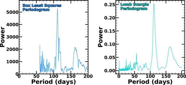
Figure 3. BLS (left) and Lomb–Scargle periodograms (right) for the full V- and g-band ASAS-SN light curve. The peak corresponding to maximum power of the BLS periodogram occurs at 111.22 ± 2.5 days, and the peak of the Lomb–Scargle periodogram occurs at 111.63 days.
Download figure:
Standard image High-resolution imageUsing a mean period leads to significant residuals between the observed and calculated peak times, as shown in the O − C diagram of Figure 4. We used the expression t0 = 28.00 + 111.23n, where n is the number of cycles, to determine the calculated times of each peak assuming a constant period. Comparing the observed times to these calculated times in JD-2456850 results in the O
−
C values shown as points in Figure 4. Such a quadratic trend is indicative of a period derivative, so the O
−
C residuals motivated the need to fit the peak arrivals with an expression including a period derivative. The period is defining the rate of change of the phase, d
ϕ/dt = 2π/P. Rearranging, integrating, and expressing in terms of n results in the expression  , where
  . Working to the third order of the expansion and inverting the polynomial, the time of the nth transient peak is

where t0 is a reference time, P0 is the “mean” period,  is the period derivative, and n is the peak number starting from the first peak set as n = 0. This expression differs from Equation (1) in Burderi et al. (2010) because the calculation was carried out to the third order instead of stopping with the quadratic (n2) term. The n2 term is not presently important for the O
−
C residuals. We use MCMC estimates for the 1σ parameter uncertainties. When fitting without a
is the period derivative, and n is the peak number starting from the first peak set as n = 0. This expression differs from Equation (1) in Burderi et al. (2010) because the calculation was carried out to the third order instead of stopping with the quadratic (n2) term. The n2 term is not presently important for the O
−
C residuals. We use MCMC estimates for the 1σ parameter uncertainties. When fitting without a  initially, we found the best-fit parameter P0 = 111.20 ± 0.06 days but the fit returns a reduced χ2 of 9.75 for 14 degrees of freedom (dof). The fit noticeably improved when including a
  with t0 = 3.4
 days, P0 = 114.6 ± 0.3 days,
  = −0.0021 ± 0.0002, and a reduced χ2 of 2.07. This fit is shown in Figure 4 as the solid line. If we expand the time of peak uncertainties in quadrature by 0.63 days to have a χ2 per degree of freedom of unity, we find best-fit parameters t0 = 5.9 ± 2.7 days, P0 = 114.2 ± 0.4 days, and
  = −0.0017 ± 0.0003. This fit is shown by Figure 4 as the dashed line and we use it as our standard model. For this model, the next two outbursts are predicted to peak in the optical on MJD 59099.9 ± 1.1 and MJD 59210.0 ± 1.4, which correspond to 2020 September 7.4 ± 1.1 and 2020 December 26.5 ± 1.4.
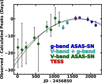
Figure 4. The O
−
C residuals comparing the observed peak time for each outburst with the estimated peak if we assume a constant period. The parabolas show the predictions from the models, including a  either with the assumed (solid) or rescaled (dashed) uncertainties for the times of peak.
Download figure:
Standard image High-resolution imageThe V- and g-band ASAS-SN light curves for ASASSN-14ko stacked using the phasing of this model are shown in Figure 5 along with the TESS light curve. Including the  significantly reduces the scatter between the stacked light curves. We also binned these stacked light curves. As is apparent in the right panel of Figure 5, the peak times are closely aligned across these three filters and the light-curve morphologies are similar between peaks and these filters. The outbursts are characterized by a fast rise to the peak followed by a shallower decline.
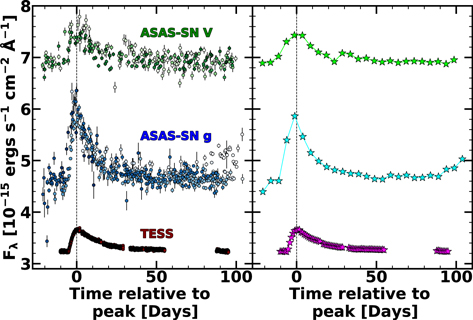
Figure 5. The stacked ASAS-SN V-band (green), ASAS-SN g-band (blue), and TESS (maroon) light curves as a function of phase. The light curves are offset for clarity and the data of each phase are given a different shade of color. The right panel shows the phase-stacked light curves binned at 5 day intervals for ASAS-SN and binned at 1 day intervals for TESS. The outburst peaks align across these filters and the shapes are similar.
Download figure:
Standard image High-resolution imageThe Catalina Real-Time Transient Survey (CRTS; Drake et al. 2009) data contain observations spanning 9 yr prior to the start of the ASAS-SN V-band light curve. However, the quality of the CRTS data made it difficult to identify prior outburst peaks relative to the quiescent baseline. The CRTS photometry includes flux from the entire host galaxy since it uses source extraction (Bertin & Arnouts 1996) rather than image subtraction. Since the host galaxy is bright and spatially large, it is difficult to recognize prior outbursts. We also found that data from the ASAS (Pojmanski 1997) were not useful for identifying earlier outbursts and we could find no other earlier data.
4.2. TESS Light-curve Analysis
The TESS light curve of ASASSN-14ko’s 2018 November outburst provides a unique view of the morphology of the outburst. Because TESS observed ASASSN-14ko over three consecutive sectors, the light curve captures the pre-outburst quiescence, the full rise to peak, and the full decline back to quiescence. Motivated by Holoien et al. (2019b) and Fausnaugh et al. (2021), we first characterized the early-time rise of ASASSN-14ko with a power-law model of


consisting of residual background z, the time of rise t1, a flux scale h, and the power-law index α. We used the package SciPY. OPTIMIZE. CURVE _FIT's (Virtanen et al. 2020) trust region reflective method to obtain a best-fit model with parameters z = − 0.02 ± 0.001 erg s−1 cm−2 Å−1, h = 0.1 ± 0.01 erg s−1 cm−2 Å−1, t1 = 2458429.7 ± 0.05 JD, and α = 1.01 ± 0.07. This fit is shown as the red curve in Figure 6. For this fit we inflated the error bars in quadrature by 0.011 erg s−1 cm−2 Å−1 in order to make the reduced χ2 of the fit unity for 160 dof. The high photometric precision of TESS shows that the early-time rise was smooth, and that the time to peak in the TESS filter was 5.60 ± 0.05 days from t1 when measuring the peak from the data binned at 8 hr intervals.
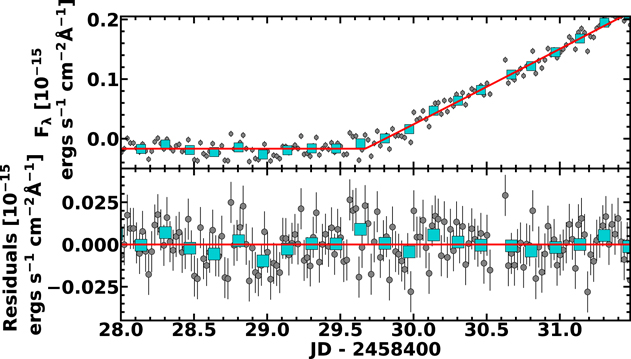
Figure 6. Rising phase of the TESS image subtraction light curve. The best-fit power-law model for the rise until JD-2458431.5 is shown in red. The bottom panel shows the flux residuals. The TESS data binned by 4 hr are shown by turquoise squares.
Download figure:
Standard image High-resolution imageThree TDEs have estimates of α, all of which are steeper. The first TDE detected by TESS was ASASSN-19bt, which had a power-law index of α = 2.10 ± 0.12 (Holoien et al. 2019b). ASASSN-19dj had α = 1.9 ± 0.4 using the ASAS-SN light curve (Hinkle et al. 2021). Values of α ∼ 2 are similar to the fireball model used for the early-time evolution of SNe (Riess et al. 1999; Nugent et al. 2011). The third example, AT2019qiz, had a still steeper power-law index rise of α = 2.8 ± 0.3 (Nicholl et al. 2020).
The photometric precision of the TESS light curve also reveals that the decline was also remarkably smooth, as shown in Figure 7. Since the rate of the decline in partial TDEs is predicted to be steeper than the canonical t−5/3 model, we followed the method in Holoien et al. (2019b) and fit the TESS light curve starting from 5 days after the peak as

with t0 being the time of disruption, constrained to be before the start of the rise, t1, determined above. We again inflated the error bars in quadrature by 0.014 erg s−1 cm−2 Å−1 in order to make the reduced χ2 unity for 2611 dof. The best-fit power law has the parameters t0 = 2458429.69 ± 0.48 JD, which corresponds to the start of the rise, z = − 0.02 ± 0.001 erg s−1 cm−2 Å−1, h = −8.77 ± 1.19 erg s−1 cm−2 Å−1, and α = −1.33 ± 0.03. As seen in Figure 7, this smooth power law describes the decline well. The exponent, far from being steeper than the canonical α = −5/3 = −1.66, is actually shallower.
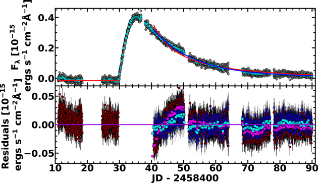
Figure 7. Declining phase models of the TESS light curve starting 5 days past the peak. The best-fit power-law decline is shown in red and the best-fit exponential decline is shown in blue. The TESS data binned in 8 hr intervals are shown by turquoise squares. The bottom panel shows the residuals of the fits color coded by model. Magenta and cyan squares show the residuals of the power-law decline and exponential decline compared to the binned TESS data, respectively.
Download figure:
Standard image High-resolution imageWe also fit the decline as an exponential decay of the form

which returns the best-fit parameters a = 0.31 ± 0.001 erg s−1 cm−2 Å−1, τ = 12.85 ± 0.11 days, and c = 0.01 ± 0.001 days. We set tpeak to the peak of the TESS light curve since its value is degenerate with the other parameters. This model has a reduced χ2 value of 0.65 for the same uncertainties. The exponential decline is, therefore, a better representation of the decline than the power-law decay model. Since starting the fit 5 days after the peak is somewhat arbitrary, Table 4 gives the results for fits starting 5, 10, 15, and 20 days after the peak all for the same error model. The fit parameters are relatively stable and the exponential model is always the better fit.
Table 4. Best-fit Parameters for the Power-law and Exponential Decline Models of the TESS Light Curve Starting the Fits for Different Numbers of Days After Peak
| Power-law Decline | ||||
|---|---|---|---|---|
| Fit Start Time from Peak (days) | t0 (JD–2458400) | h (erg s−1 cm−2 Å−1) | α | χ2 per dof |
| 5 | 29.69 ± 0.48 | −8.77 ± 1.19 | −1.33 ± 0.03 | 1.08 |
| 10 | 29.70 ± 1.11 | −10.00 ± 2.51 | −1.35 ± 0.06 | 0.91 |
| 15 | 29.70 ± 3.03 | −10.00 ± 5.76 | −1.38 ± 0.13 | 0.72 |
| 20 | 29.70 ± 6.23 | −10.00 ± 10.90 | −1.40 ± 0.24 | 0.70 |
| Exponential Decline | ||||
| Fit Start Time from Peak (days) | a (erg s−1 cm−2 Å−1) | τ (days) | c (days) | χ2 per dof |
| 5 | 0.31 ± 0.001 | 12.85 ± 0.11 | 0.01 ± 0.001 | 0.65 |
| 10 | 0.22 ± 0.001 | 11.06 ± 0.14 | 0.02 ± 0.001 | 0.60 |
| 15 | 0.13 ± 0.001 | 12.11 ± 0.33 | 0.01 ± 0.001 | 0.56 |
| 20 | 0.09 ± 0.001 | 10.83 ± 0.44 | 0.02 ± 0.001 | 0.55 |
Note. z for the power-law decline was −0.02 ± 0.001 erg s−1 cm−2 Å−1 for 5 and 10 days past and −0.01 ± 0.001 erg s−1 cm−2 Å−1 for 15 and 20 days post-peak.
Download table as: ASCIITypeset image
4.3. 2020 May Outburst
The 2020 May outburst was the first to be predicted in advance, and it occurred as expected. We initially predicted the outburst to peak on MJD 58990.2 ± 1.9 based on our preliminary period estimate using the periodogram. The ASAS-SN g-band light curve actually peaked on MJD  , as shown in the last panel of Figure 2, consistent with the prediction.
We requested Swift observations to monitor the outburst along with the LCOGT and amateur ground-based data. The non-host-subtracted light curves along with the X-ray hardness ratios are shown in Figure 8. Unfortunately, the ground-based observations were severely impacted by COVID-19 closures and the impending Sun constraint. The ASAS-SN light curve in the month leading up to the 2020 May outburst had a gap due to these closures. Observations were collected by the amateur astronomers, but large gaps exist in those light curve due to weather closures. The combined data set was processed as uniformly as possible, but the scatter prevents unambiguous interpretations of the multiband light curve.
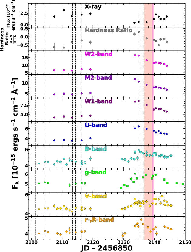
Figure 8. Non-host-subtracted photometry of the 2020 May outburst. ASAS-SN g-band photometry is represented as squares, Swift data as circles, LCOGT data as pentagons, and data from amateur observatories as diamonds. B-band, g-band, and V-band data taken from different telescopes on the same day were averaged. Swift B- and V-band data were converted to Johnson B and V magnitudes before being converted to flux to enable direct comparison with the ground-based data. Error bars are plotted but are frequently smaller than the size of the points. The red-shaded region denotes the time of the ASAS-SN g-band peak on JD- and the magenta vertical solid line shows the predicted peak for our model with a period derivative, as was also shown in Figure 2. The vertical dashed lines indicate the observation times of the LCOGT spectra shown in Figure 14.
Download figure:
Standard image High-resolution imageThe most interesting feature of Figure 8 is that we can clearly see a wavelength dependence on the flux peak. While the rise was fully observed for the B band and longer wavelengths, the UV- and U-band data clearly peaked at still earlier times and the optical bands lagged the UV bands by several days. This is also apparent in the blackbody fits to the host-subtracted Swift data shown in Figure 9 and Table 5. The peak blackbody luminosity and temperature occurred approximately 4 days prior to the ASAS-SN g-band peak. However, the blackbody radius remained roughly consistent over time.
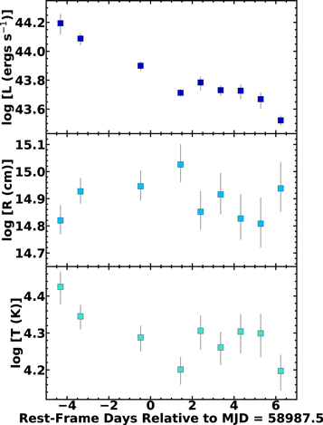
Figure 9. Evolution of the UV/optical blackbody luminosity (top panel), radius (middle panel), and temperature (bottom panel) during the 2020 May outburst based on the host-subtracted Swift data and shown in Table 5. The time is relative to the g-band peak on MJD 58987.5. The luminosity and temperature peak occurred several days prior to the g-band peak.
Download figure:
Standard image High-resolution imageTable 5. Blackbody Luminosity, Radius, and Temperature During the 2020 May Outburst Derived from the Host-subtracted Swift Data
| MJD | log [L (erg s−1)] | log [R (cm)] | log[T (K)] |
|---|---|---|---|
| 58969.0 | 43.1 
| 15.49 
| 3.81 
|
| 58983.0 | 44.19 
| 14.82 
| 4.42 
|
| 58984.0 | 44.09 
| 14.93 
| 4.34 
|
| 58987.0 | 43.90 
| 14.95 
| 4.29 
|
| 58989.0 | 43.71 
| 15.03 
| 4.20 
|
| 58990.0 | 43.78 
| 14.85 
| 4.31 
|
| 58991.0 | 43.73 
| 14.92 
| 4.26 
|
| 58992.0 | 43.73 
| 14.83 
| 4.30 
|
| 58993.0 | 43.67 
| 14.81 
| 4.30 
|
| 58994.0 | 43.52 
| 14.94 
| 4.20 
|
Download table as: ASCIITypeset image
The Swift XRT X-ray light curve did not follow the same trend. At peak optical flux, the X-ray flux had dropped by a factor of ∼4 and the spectrum became harder. The hardening of the emission could mean that the effective radius for the X-ray emission is shrinking, that a harder power-law flux component is increasing, or there is additional obscuration that is attenuating the soft X-ray photons. However, during the outburst peak, the hardness ratio decreased, making it difficult to reconcile the X-ray evolution with the UV/optical.
The UV/optical and X-ray SEDs at two epochs during the 2020 May outburst are shown in Figure 10. The two epochs correspond to 4 days before and 7 days after the ASAS-SN g-band peak, which approximately corresponds to the UV peak and post-maximum UV quiescence. The peak luminosity is roughly 1% of the Eddington luminosity derived in Section 3.
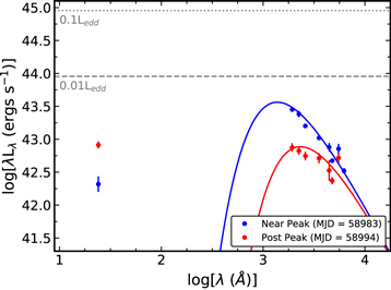
Figure 10. Host-subtracted SED at two epochs during the 2020 May outburst. The first epoch on MJD 58983 (blue) is 4 days prior to the g-band peak on MJD 58987.5. The second epoch on MJD 58994 (red) is 7 days after the g-band peak. For the UV/optical, the data are shown as points, while the lines represent the best-fit blackbody components. The X-ray luminosities are shown at the center of the 0.3–10 keV band over which the luminosity is determined. The gray-dashed and gray-dotted lines are 1% and 10%, respectively, of the Eddington luminosity for an SMBH of mass 7.2 × 10⁷ M⊙.
Download figure:
Standard image High-resolution image4.4. Comparison to TDEs
We first compared each of ASASSN-14ko’s outbursts to the peak luminosity-decline rate relation for previously studied TDEs (Hinkle et al. 2020). This relation describes a correlation between the peak luminosity and its decline luminosity over 40 days. First, we bolometrically corrected the ASAS-SN V and g bands, and TESS photometry using a temperature of 28,800 K, which is the median temperature of the most recent outburst based on the Swift data. Then, following the procedure of Hinkle et al. (2020), we calculated a peak luminosity and the decline rate over 40 days for each outburst. In Figure 11, we compare the peak luminosity and decline rate of these outbursts to known TDEs. Even though the power-law slope of the decline is shallower than t−5/3 (Section 4.2), the actual decline rate is steeper than all TDEs of similar luminosity.
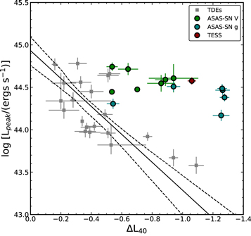
Figure 11. Peak luminosity-decline rate for ASASSN-14ko’s outbursts were compared to 21 previously studied TDEs. Individual ASAS-SN V (green circles), ASAS-SN g (teal circles), and TESS (red circle) epochs are shown along with the TDEs analyzed by Hinkle et al. (2020) represented as gray squares. The black solid line is the best-fit line for the TDEs and the black-dashed lines are the allowed range of uncertainty from the best-fit line.
Download figure:
Standard image High-resolution imageWe directly compare the TESS light curves of ASASSN-14ko and ASASSN-19bt (Holoien et al. 2019b) in Figure 12 in order to compare ASASSN-14ko’s flare timescale and morphology to another TDE with well-sampled early-time light curves. ASASSN-14ko clearly evolves much more rapidly than ASASSN-19bt, with both a more rapid rise and a more rapid decline. However, the overall morphologies of the declining light curves are very similar if we compress the time relative to peak of ASASSN-19bt by 30% in order to align the light-curve declines as shown in the right panel of Figure 12.
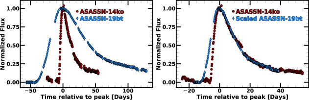
Figure 12. The TESS light curves of ASASSN-14ko (red circles) binned in 4 hr intervals and ASASSN-19bt (blue diamonds) binned in 16 hr intervals. The left panel shows the light curves as observed, and the right panel shows the ASASSN-19bt light curve compressed in time by 30% to align the light-curve declines.
Download figure:
Standard image High-resolution image5. Analysis of Spectra
5.1. Evolution of the Optical Spectra
We used optical spectra observed at different points in time and shown in Figure 13 to first classify ASASSN-14ko using standard Baldwin, Phillips, & Telervich (BPT) diagnostics (Baldwin et al. 1981; Veilleux & Osterbrock 1987; Kauffmann et al. 2003; Kewley et al. 2001, 2006). The 1996 spectrum and a weighted average of the 2014–2015 spectra both have line ratios consistent with AGNs. The measured ratios are given in Table 6.
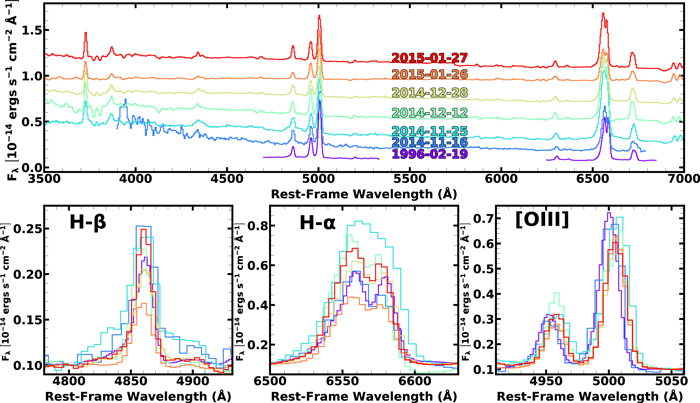
Figure 13. Spectra of ESO 253-G003 showing the change in the Balmer emission-line profiles. The earliest epoch from 1996 February 19 (Kewley et al. 2001) is shown in violet. Subsequent spectra were taken after the discovery of ASASSN-14ko, including the spectrum reported in Holoien et al. (2014a) and five epochs from PESSTO. The spectra have been scaled using mapspec to put all of them onto a common flux scale. The spectra shown at top have been shifted for clarity. The bottom panels have been scaled to a common continuum.
Download figure:
Standard image High-resolution imageTable 6. Diagnostic Emission-line Ratios log10([O III]/Hβ), log10([N II]/Hα), log10([S II]/Hα), and log10([O I]/Hα) Used to Distinguish AGNs from H II Regions and Classify AGNs as Either Seyferts or Low-ionization Nuclear Emission-line Regions (LINERs; Baldwin et al. 1981; Veilleux & Osterbrock 1987; Kewley et al. 2001, 2006; Kauffmann et al. 2003)
| Ratio Diagnostic | 1996 | 2014–2015 |
|---|---|---|
| log10([O III]/Hβ) | 0.73 ± 0.04 | 0.81 ± 0.12 |
| log10([N II]/Hα) | −0.25 ± 0.03 | −0.59 ± 0.23 |
| log10([S II]/Hα) | −0.57 ± 0.03 | −0.61 ± 0.07 |
| log10([O I]/Hα) | −1.10 ± 0.03 | −1.18 ± 0.08 |
Note. The 2014–2015 ratios were measured from a weighted average of the 2014–2015 spectra.
Download table as: ASCIITypeset image
Next, we examined the evolution of the Hβ and Hα emission-line profiles. The spectra from 2014–2015 were taken after ASASSN-14ko’s optical peak, as indicated by the orange tick marks in Figure 2. Directly comparing these spectra should be done with caution because the data were taken with different instruments and long-slit setups. However, these spectra may show that the emission-line profile shapes changed during the 2014 November outburst.
We obtained five spectra with the LCOGT FLOYDS spectrograph during quiescence in 2020 April and two spectra during the optical rise of the 2020 May outburst. We compared them to determine any change in the emission-line profiles as shown in Figure 14. Due to observatory airmass constraints and ASASSN-14ko’s low position near the horizon from the Siding Spring Observatory at that time, observations were not possible past 2020 May 17. These two observations occurred 1 and 2 days before the optical peak, respectively, which coincided with the start of the decline in the UV, as shown by the vertical-dashed lines in Figure 8 and the orange tick marks in Figure 2. A noticeable feature of the spectra during outburst is a blue wing around Hβ near 4830 Å that is not present in the spectra taken during quiescence. This feature is similar to the broadened wings present in the 2014 November 16 and 2014 November 25 spectra, which were taken during an outburst optical decline. This gives further evidence that the Balmer lines change during the outburst.
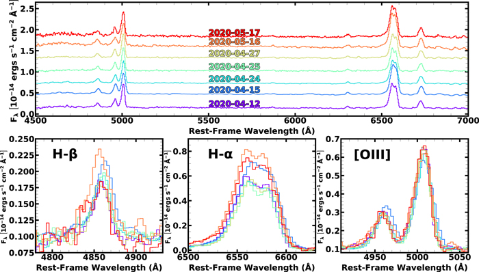
Figure 14. Spectra of ESO 253-G003 observed with the FLOYDS spectrograph at LCOGT during quiescence in 2020 April and during the 2020 May outburst. The first five spectra were obtained during quiescence and the last two spectra were obtained during the optical rise of the 2020 May outburst. The spectra have been scaled using mapspec to put all of them onto a common flux scale. The spectra shown at top have been shifted for clarity. The bottom panels have been scaled to a common continuum.
Download figure:
Standard image High-resolution imageThe similarities between the spectroscopic evolution of the two outbursts separated by nearly 6 yr indicates that the spectroscopic change during the flare may be a consistent component of these events. However, ESO 253-G003 has very complex spectroscopic structures in IFU observations (Tucker et al. 2020), which makes it difficult to interpret long-slit observations with different orientations and resolutions. The photometric and spectroscopic evolution could be closely tied, and a higher temporal resolution of upcoming outbursts may reveal further connections between the rise and decline of the photometric light curves with morphological changes in the Balmer lines.
5.2. X-Ray Analysis
We compared the two X-ray spectral epochs to characterize the X-ray emission evolution and they are shown in Figure 15. We modeled the 2015 XMM-Newton+NuSTAR spectra as a combination of a soft blackbody plus a power law. The blackbody model had a temperature of 0.15 ± 0.01 keV and the power-law model had a Γ = 0.87 ± 0.04. There is a strong 6.4 keV Fe line present that we include in the model as a Gaussian. The Swift XRT spectrum was extracted from the merged data taken from ∼30 days prior to and ∼9 days after the 2020 May flare, which corresponds to the times during both quiescence and outburst. This spectrum was best fit by a power law with  and the fit was not improved by adding an additional blackbody with a best-fit temperature of 0.13 ± 0.03 keV. The Swift spectrum had combined all the 2020 May observations because the signal-to-noise ratio of the spectrum would otherwise have been too low to assess its characteristics. With only ∼650 counts, poor statistics likely prevent any detection of the Fe line. The fit parameters are summarized in Table 7.
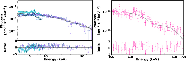
Figure 15. XMM-Newton+NuSTAR spectra (left) from MJD = 57253.6 during a period of quiescence compared to the recent Swift spectra (right). The recent Swift observations do not show the Fe line around 6.4 keV, but this is likely due to the low signal-to-noise ratio.
Download figure:
Standard image High-resolution imageTable 7. Best-fit Parameters for the Swift and XMM-Newton+NuSTAR X-Ray Spectra
| Instrument | kT (keV) | Blackbody Normalization (K) | Photon Index Γ | χ2 per dof |
|---|---|---|---|---|
| Swift | 0.13 ± 0.03 |

|

| 1.07 |
| XMM+NuSTAR | 0.15 ± 0.01 |

| 0.87 ± 0.04 | 1.64 |
Note. Both models used a redshift of 0.0425 and a neutral hydrogen column density NH of 3.5 × 1020 cm−2 frozen to the Galactic column density (HI4PI Collaboration et al. 2016). The XMM-Newton+NuSTAR spectrum included a Gaussian line energy of 6.39 ± 0.03 keV to capture the 6.4 keV Fe line. The Swift fit had 56 dof and the XMM-Newton+NuSTAR fit had 470 dof
Download table as: ASCIITypeset image
The XMM-Newton spectrum was taken during a period when the optical flare was quiescent, however, the flux derived from the XMM-Newton spectrum is similar to what we observed with Swift. The similarities between the Swift spectrum and the XMM-Newton spectrum may indicate that even during times around the UV peak, the average properties of the X-ray emission during 2020 May may not have changed significantly from the properties of the deep XMM-Newton observation. Future observations with a better signal to-noise ratio will be essential to disentangle potential evolution of X-ray emission between the quiescence and outburst. There are nine epochs of XMM-Newton slew observations of this galaxy observed between 2007 and 2019. However, given the sparse sampling and low signal-to-noise ratio, there is no obvious pattern after phase folding these data.
6. Discussion
Here, we discuss several scenarios for ASASSN-14ko’s periodic outbursts and some of their problems. We consider the possibilities that ASASSN-14ko is a sub-parsec SMBH binary system, an SMBH and perturbing massive star binary system, and finally, a repeating partial TDE. We do not consider stellar origins for the outbursts. A Galactic source is ruled out because the changes in the Balmer line strengths and profiles during outburst occur at the redshift of the host Seyfert Type 2 galaxy ESO 253-G003. At the redshift of the host, the peak luminosities are similar to those of luminous SNe and so are too high for non-explosive stellar transients. The many quasiperiodic repetitions of similar luminosity rule out explosive possibilities. This appears to leave only phenomena associated with a central SMBH as possible explanations. In addition, models describing EMRIs indicate that they produce flares with a typical recurrence time on the order of 105 yr with the shortest on the order of a decade (Metzger & Stone 2017). Since ASASSN-14ko’s period is ∼30 times shorter, we do not consider the EMRIs model further for ASASSN-14ko.
6.1. ASASSN-14ko as an SMBH Binary System
As discussed in the introduction, apparently periodic emission from AGNs is frequently interpreted as evidence for an SMBH binary. However, there are three main inconsistencies with this scenario for ASASSN-14ko: (1) the period derivative; (2) the short lifetime of such a binary, and (3) the lack of velocity shifts. We will scale the results for black hole masses of  ,
,  and a period of
  days.
days.
6.2.
Due to the emission of gravitational waves, the binary will have a period derivative of

where  is the dependence on the orbital ellipticity e, and a time to merger of

where  (Peters 1964). The first problem is that the observed period derivative is over an order of magnitude larger than the scaling in Equation (6) for black holes in a circular orbit. This can be solved only by substantially increasing the mass of at least one of the black holes, or by making the orbit significantly elliptical. Both of these solutions to the mismatch in period derivatives will exacerbate the next two problems by reducing the binary lifetime and increasing the binary velocities. If the solution is to change the masses, the lines must be formed around the less massive SMBH, which also exacerbates the velocity problem.
The second problem is that finding a binary so close to merging is very improbable. The first way to phrase this is through what it requires for the properties of SMBH binaries in other galaxies. The number density of L* galaxies is roughly n ≃ 0.01h3 Mpc−3 (e.g., Kochanek et al. 2001), so there are roughly Ng
≃ 3 × 10⁵ such galaxies inside the distance to ESO 253-G003. To have one system merging in the next t0 = 1000 yr implies that all of these galaxies must contain binaries that will merge in the next Ng
t0 ≃ 300 million yr. This in turn implies that they must all have orbital periods shorter than ∼ yr, which would seem to make the problem of finding binary SMBH systems rather trivial rather than being as difficult as it appears to be in practice. The second way to phrase the problem is that if there is one SMBH binary with a period <1/3 yr in this volume, there are 38/3 = 19 with periods <1 yr, 350 with periods <3 yr, and 8700 with periods <10 yr.
The third problem for an SMBH binary is the high velocity scale, with

for circular orbits. While our phase sampling is poor, we arguably can set a limit on any Hβ line shifts of <50 Å, which corresponds to a velocity shift limit of <3000 km s−1. If our estimate of  is correct, this problem cannot be solved by reducing the masses or invoking a large mass ratio with the emission lines being formed by material associated with the more massive SMBH. Similarly, raising the ellipticity to solve the
  problem makes this problem worse because of the higher velocities at the pericenter compared to a circular orbit of the same period. The velocity problem can only be solved by making the system nearly face-on or by relying on the poor spectral sampling to hide the velocity shifts.
6.3. ASASSN-14ko as an SMBH with a Perturbing Star
Rather than a binary system with two SMBHs, the periodic outbursts could be driven by a star orbiting a single SMBH. Because stars are far more common than SMBHs and the gravitational wave merger lifetimes are now far longer, the probability argument against an SMBH binary is removed. The long gravitational wave merger time does mean that the observed  must have a different origin such as viscous interactions between the disk and the star, although estimating this effect is nontrivial.
We now assume a star of mass  and radius
  orbiting a black hole of mass
  . There are three length scales of immediate interest, and we show their relative values and their dependence on SMBH mass in Figure 16. The Schwarzschild radius of the black hole is

the tidal (Roche) radius to disrupt the star is

and the orbital semimajor axis is

Finally, for a pericentric radius Rp , the ellipticity of the orbit is

For some star/SMBH scenarios, the true period would be twice the observed period, which would increase the semimajor axis by 0.2 dex.
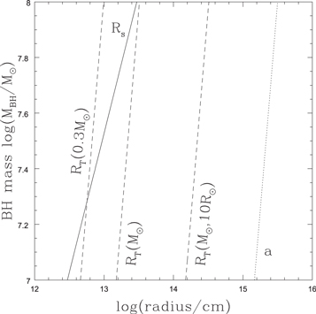
Figure 16. The Schwarzschild radius (Rs , solid), semimajor axis (a, dotted), and several tidal radii (RT , dashed) as a function of SMBH mass MBH. The tidal radii are for a 0.3M⊙ main-sequence star (RT (0.3M⊙)), the Sun (RT (1.0M⊙)), and a star with the mass of the Sun and a radius of 10R⊙ (RT (M⊙, 10R⊙). On these logarithmic scales, the effects of spin on the BH horizon and the tidal limits are modest.
Download figure:
Standard image High-resolution imageFrom Figure 16, it can be seen that there is no problem having a main-sequence star orbiting an SMBH in this mass range without serious tidal effects provided the orbital ellipticity is moderate. Particularly over many orbits, there would be some relativistic effects. For example, the orbital precession per orbit is

for a Schwarzschild black hole. This means that we would expect systematic changes with time independent of the mechanism driving the flares.
If the star is not being tidally disrupted, then the flares must be driven by periodic disturbances of the accretion flows as the star passes through the accretion disk. However, a star simply embedded in the disk would represent a continuous perturbation that is unlikely to drive periodic flares. Flaring would seem to require a stellar orbit at a significant inclination angle relative to the disk. The star would then make two passages through the disk per orbit, so the orbital period would likely be twice the flare period.
Each orbit would produce a pair of flares with the spacing dependent on the orbital eccentricity and the argument of periapsis (ω) relative to the accretion disk. The separation between pairs will increase as the orbit becomes more eccentric. While eccentric orbits with ω near 0 or π can have equally spaced encounters, the star will encounter the disk at different radii/temperatures. Given that the flare spacing, profiles, and amplitudes are all essentially constant between cycles, a perturbing star would seem be required to be on an inclined but nearly circular orbit. Even then, the similarity of the flares seems odd because one would expect encounters with the star moving away from the observer and into the disk to differ from the reverse, except for nearly edge-on viewing angles. In Figure 17, it can be seen that the even and odd flare profiles are very similar in amplitude, shape, and duration, which is difficult to reconcile with this model. Finally, while an inclined, circular orbit of a star orbiting an SMBH might be able to perturb the accretion disk with the right frequency, there is no obvious timescale in disks to then make the flares so short in duration.
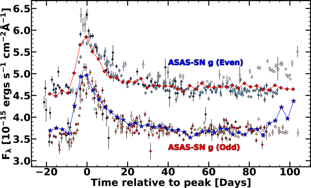
Figure 17. The stacked ASAS-SN g-band light curves separated by even (blue) and odd (red) outbursts as a function of phase. The light curves are offset for clarity and the data of each phase are given a different shade of color. The binned even light curve, shown by star symbols, is superimposed over the odd light curves, and vice versa, with the binned odd light curve shown by diamond symbols.
Download figure:
Standard image High-resolution image6.4. ASASSN-14ko as a Repeated Partial TDE
A third possibility to explain ASASSN-14ko’s periodic outbursts is as a repeating TDE that is partially disrupted after each passage close to the central SMBH. While it requires fine-tuning to have a main-sequence star pass close to its tidal limit but remain outside the SMBH horizon, we can see from Figure 16 that it is relatively easy for an evolved star on an elliptical orbit to do so. As discussed in the Introduction, giants are also the most likely candidates for partial disruptions that could power periodic flares. MacLeod et al. (2012) and Guillochon & Ramirez-Ruiz (2013) found that the star will begin to lose mass once β = RT /Rp < 0.5.
The peak luminosities of the flares, Lp
≃ 5 × 1044 erg s−1 correspond to the peak accretion rates of  yr−1, where
 = 0.1
0.1 is the accretion efficiency. If the peaks last ∼10 days, the accreted mass of
 is certainly low enough to allow repeated outbursts on this scale. Note, however, that these accretion rates are significantly higher than envisioned by MacLeod et al. (2013) and the time scales are much shorter.
Ryu et al. (2020) found that the change in the orbital specific energy of the star in a partial disruption is f ∼ 10−3 of the specific energy scale  of the stripped debris. They found both positive and negative energy changes, so there is no prediction of the sign of the changes. The period derivative measured in Section 4.1 implies a change in the orbital specific energy of
  . This means that we should expect a period derivative of

For f ∼ 10−3, this implies  with relatively little sensitivity to the exact values of the parameters and remarkably close to the measured period derivative. The agreement is perhaps more remarkable because the Ryu et al. (2020) simulations were for a single pericentric passage of a main-sequence star on an initially parabolic orbit, rather different from the orbit required here. However, the orbit of the puffy stellar merger remnant in Figure 13 (top) of Antonini et al. (2011) has a semimajor axis shrinking as Δa/a ∼ 10−3 per orbit, which is the same order of magnitude. The example in the lower panel of this figure shows very little orbital evolution but also shows very little ongoing mass loss. Note that the orbital changes essentially occur with the pericenter fixed because the tidal interactions are only important at the pericenter. Because the structure of the star must be changing with each pericentric passage due to the mass loss, torques, and heating,
  presumably cannot be constant on longer time scales.
The partial TDE hypothesis also seems better able to explain the similarity of the flares since each pericentric passage is almost identical in geometry to the previous and the required mass-loss rates appear to be modest. However, they cannot truly be identical since the orbital geometry must slowly change due to precession (relativistic and tidal) and the mass lost over tens of encounters ceases to be modest. Overall, the repeating, partial TDE interpretation seems most consistent with the available observations.
7. Summary
Although ASASSN-14ko was first thought to be an SN, the subsequent 6 yr of ASAS-SN V- and g-band data show that the flares occur at regular intervals. The 17 flares observed to date are well modeled using a period of P0 = 114.2 ± 0.4 days and period derivative of  . Adopting this model, the next two flares will peak in the optical on UT 2020 September 7.4 ±1.1 and UT 2020 December 26.5 ±1.4. The 2020 September flare peak occurred as predicted (A. V. Payne et al. 2021 in preparation).
In addition to ASAS-SN, ATLAS, and Swift multiwavelength photometric data, TESS observed ASASSN-14ko during its 2018 November outburst. The TESS light curve has a decline rate that is dissimilar to previously studied TDEs and a rapid rise to peak occurring over 5.60 ± 0.05 days. The TESS data also show that the rise and decline were smooth and lack short-timescale variability. The individual outbursts are morphologically very similar over the 6 yr baseline of observations. While a host of problems interfered with studying the 2020 May outburst well, there was clear evidence that the outburst peaks a few days earlier in the UV than in the optical. Spectra taken during and prior to the 2020 May outburst revealed morphological changes around Hβ during the flare, which was similar to what occurred during the 2014 outburst. This suggests that morphological changes in the emission lines are consistently associated with the optical outbursts over time. We examined several possible scenarios to explain the cause of this AGNs’ unusual behavior, including the presence of an SMBH binary, an SMBH plus a perturbing massive star, or a repeating partial TDE. Between these scenarios, we favor a repeating partial TDE. We believe that any stellar transients or explosions whether Galactic or in the host are ruled out. The most important next step is to time and study the flares more closely across the electromagnetic spectrum. The relatively short period and system brightness make this relatively easy. ASASSN-14ko will be observed by TESS again in Sectors 31–33 during the predicted 2020 December outburst. These observations will give further constraints on the nature of these outbursts and presents a unique opportunity to do a detailed reverberation mapping analysis of the system.
Software: FTOOLS (Blackburn 1995), NuSTAR Data Analysis Software (v1.8.0), mapspec (Fausnaugh et al. 2016), HEAsoft (HEASARC 2014), IRAF (Tody 1986, 1993), AGNfitter (Calistro Rivera et al. 2016), astroML (Vanderplas et al. 2012).
We thank the anonymous referee whose comments improved the paper. We also thank Chris Ashall, Patricia T. Boyd, Bradley Peterson, Brian Metzger, Richard Pogge, Nicholas Stone, and Jennifer van Saders for helpful discussions.
We thank the Las Cumbres Observatory and its staff for its continuing support of the ASAS-SN project. ASAS-SN is supported by the Gordon and Betty Moore Foundation through grant GBMF5490 to the Ohio State University, and NSF grants AST-1515927 and AST-1908570. Development of ASAS-SN has been supported by NSF grant AST-0908816, the Mt. Cuba Astronomical Foundation, the Center for Cosmology and AstroParticle Physics at the Ohio State University, the Chinese Academy of Sciences South America Center for Astronomy (CAS- SACA), and the Villum Foundation.
A.V.P. acknowledges support from the NASA Fellowship through grant 80NSSC19K1679. B.J.S., C.S.K., and K.Z.S. are supported by NSF grant AST-1907570. B.J.S. is also supported by NASA grant 80NSSC19K1717 and NSF grants AST-1920392 and AST-1911074. C.S.K. and K.Z.S. are supported by NSF grant AST-181440. K.A.A. is supported by the Danish National Research Foundation (DNRF132). M.A.T. acknowledges support from the DOE CSGF through grant DE-SC0019323. Support for J.L.P. is provided in part by FONDECYT through the grant 1191038 and by the Ministry of Economy, Development, and Tourism’s Millennium Science Initiative through grant IC120009, awarded to The Millennium Institute of Astrophysics, MAS. T.A.T. is supported in part by Scialog Scholar grant 24215 from the Research Corporation. Parts of this research were supported by the Australian Research Council Centre of Excellence for All Sky Astrophysics in 3 Dimensions (ASTRO 3D), through project number CE170100013.
Footnotes
- 25
- 26
- 27
- 28
- 29
- 30
- 31