Abstract
We report on VLT/FORS2 imaging polarimetry observations in the RSpecial band of WISE J011601.41–050504.0 (W0116–0505), a heavily obscured hyperluminous quasar at z = 3.173 classified as a Hot Dust-obscured Galaxy (Hot DOG) based on its mid-IR colors. Recently, Assef et al. identified W0116–0505 as having excess rest-frame optical/UV emission and concluded that this excess emission is most likely scattered light from the heavily obscured AGN. We find that the broadband rest-frame UV flux is strongly linearly polarized (10.8% ± 1.9%, with a polarization angle of 74° ± 9°), confirming this conclusion. We analyze these observations in the context of a simple model based on scattering either by free electrons or by optically thin dust, assuming a classical dust torus with polar openings. Both can replicate the degree of polarization and the luminosity of the scattered component for a range of geometries and column densities, but we argue that optically thin dust in the ISM is the more likely scenario. We also explore the possibility that the scattering medium corresponds to an outflow recently identified for W0116–0505. This is a feasible option if the outflow component is biconical with most of the scattering occurring at the base of the receding outflow. In this scenario, the quasar would still be obscured even if viewed face-on but might appear as a reddened type 1 quasar once the outflow has expanded. We discuss a possible connection between blue-excess Hot DOGs, extremely red quasars, reddened type 1 quasars, and unreddened quasars that depends on a combination of evolution and viewing geometry.
Original content from this work may be used under the terms of the Creative Commons Attribution 4.0 licence. Any further distribution of this work must maintain attribution to the author(s) and the title of the work, journal citation and DOI.
1. Introduction
Hot Dust-obscured Galaxies (Hot DOGs) are a population of hyperluminous obscured quasars (Eisenhardt et al. 2012; Wu et al. 2012) identified by NASA’s Wide-field Infrared Survey Explorer (WISE; Wright et al. 2010). Hot DOGs comprise some of the most luminous galaxies in the universe, most with LBol ≳ 1013 L⊙ and ∼10% with bolometric luminosities exceeding 1014 L⊙, without signs of gravitational lensing (Tsai et al. 2015). A number of studies have identified a hyperluminous, highly obscured active galactic nucleus (AGN) as the primary source of the luminosity in these objects (e.g., Eisenhardt et al. 2012; Assef et al. 2015). This obscured AGN component dominates at mid-IR wavelengths (Assef et al. 2015) but is sometimes luminous enough to dominate the emission at far-IR wavelengths as well (Jones et al. 2014; Díaz-Santos et al. 2016; Diaz-Santos et al. 2021). Hard X-ray spectra have been obtained for several Hot DOGs, leading to the conclusion that the obscuration is close to or above the Compton-thick threshold (Stern et al. 2014; Piconcelli et al. 2015; Assef et al. 2016, 2020; Vito et al. 2018). Recent studies have shown that some Hot DOGs are driving massive outflows of ionized gas (Díaz-Santos et al. 2016; Finnerty et al. 2020; Jun et al. 2020), as well as possibly molecular gas outflows (Fan et al. 2018), suggesting that the obscured, hyperluminous quasar may be in the course of shutting down star formation by removing the host galaxy gas reservoir. Additionally, a number of studies have identified that at least part of the Hot DOG population may be involved in mergers (Fan et al. 2016; Farrah et al. 2017; Assef et al. 2020), with the clearest case being the discovery that the most luminous Hot DOG may be at the center of a multiple merger system with three neighboring galaxies (Díaz-Santos et al. 2018). This could make Hot DOGs consistent with being at the blowout stage of the massive galaxy evolution scheme suggested by, e.g., Hopkins et al. (2008), although Diaz-Santos et al. (2021) recently suggested that the Hot DOG phase may be recurrent throughout the lifetime of a massive galaxy.
Hot DOGs have very distinctive UV through IR spectral energy distributions (SEDs; e.g., see Tsai et al. 2015; Assef et al. 2015). The highly obscured, hyperluminous AGN dominates the IR SEDs of these objects, as well as the bolometric luminosity output, while a moderately star-forming galaxy without significant obscuration typically dominates the UV and optical portions of the SED (see, e.g., Eisenhardt et al. 2012; Jones et al. 2014; Assef et al. 2015). Assef et al. (2016) studied the UV through mid-IR SEDs of a large number of Hot DOGs and identified eight objects that showed considerably bluer SEDs. They dubbed this subsample blue-excess Hot DOGs, or BHDs. They found that the excess blue emission had a power-law shape and was best modeled by the emission from an unobscured or lightly obscured AGN accretion disk with ∼1% of the luminosity of the obscured AGN responsible for the IR emission. Assef et al. (2016) discussed the possible origins of this excess blue emission and presented a detailed study of one BHD, WISE J020446.13–050640.8 (hereafter W0204–0506; z = 2.100). They concluded that the most likely source of the blue-excess emission in W0204–0506 is light from the highly obscured, hyperluminous AGN scattered into our line of sight. In a follow-up study, Assef et al. (2020) presented further observations of this source, as well as a detailed study of two more BHDs, WISE J011601.41–050504.0 (hereafter W0116–0505; z = 3.173) and WISE J022052.12+013711.6 (hereafter W0220+0137; z = 3.122). They also concluded that the most likely source of the excess blue emission in all three sources is scattered light from the obscured AGN, although a contribution from star formation could not be completely ruled out, particularly in the case of W0204–0506.
A possible way to differentiate between the star formation and scattered-light origins of the blue excess is through linear polarization in the UV, since a high degree of polarization would be expected for the latter scenario but not for unobscured star formation. There is a rich history of detecting scattered emission in obscured AGN through their linearly polarized flux, and such observations comprise the basis of the AGN unification model (see, e.g., Antonucci & Miller 1985; Miller et al. 1991; Antonucci 1993). Furthermore, unobscured quasars do not show high polarization. Berriman et al. (1990) measured the polarization properties of 114 type 1 QSOs in the Palomar–Green Quasar Survey (Schmidt & Green 1983) and found an average polarization of 0.5% with a maximum of 2.5%. Luminous obscured quasars and radio galaxies, on the other hand, show significantly larger polarization, up to ∼20% in some cases (see, e.g., Hines et al. 1995; Smith et al. 2000; Vernet et al. 2001; Zakamska et al. 2005; Alexandroff et al. 2018).
In this paper, we present imaging polarimetric observations of W0116–0505, the brightest of the BHDs studied by Assef et al. (2020) at observed-frame optical wavelengths, carried out with the FOcal Reducer/low dispersion Spectrograph 2 (FORS2) instrument at the Very Large Telescope (VLT), finding high linear polarization and confirming that scattered-light emission is the source of the blue excess in this BHD. In Section 2, we describe these observations, as well as other supporting observations presented by previous studies. In Section 3, we discuss our linear polarization measurements. In Section 4, we discuss in more detail the supporting indirect evidence for scattered light in BHDs and the implications of the linear polarization detection on the obscuration geometry and scattering medium. Finally, in Section 5, we summarize our conclusions. All errors are quoted at the 1σ level. Throughout the paper, we assume a flat ΛCDM cosmology with H0 =67.7 km s−1 Mpc−1 and ΩM = 0.307 (Planck Collaboration et al. 2016).
2. Observations
2.1. Photometric and Spectroscopic Data
Assef et al. (2020) identified W0116–0505 as a BHD from its multiwavelength SED, shown in Figure 1. The figure also shows the best-fit model SED obtained using the templates and algorithm of Assef et al. (2010) but modified to consider a second AGN SED component (see Assef et al. 2016, 2020 for details). Briefly, the SED is modeled as a nonnegative linear combination of three empirically determined host galaxy templates (referred to as E, Sbc, and Im, as they correspond to modified versions of the Coleman et al. 1980 templates of the same name) and two AGN components. Each AGN SED component uses the same underlying template but with independent luminosity and obscuration. The latter is quantified by the color excess E(B − V) and assumes RV
= 3.1 and a reddening law equal to that of the Small Magellanic Cloud (SMC) of Gordon & Clayton (1998) at λ < 3300 Å and the Milky Way (MW) of Cardelli et al. (1989) at longer wavelengths (see Assef et al. 2010 for further details). The obscured, more luminous AGN component has intrinsic  and
and  , while the lower-luminosity, unobscured AGN component has intrinsic
  and E(B − V) < 0.02 mag.
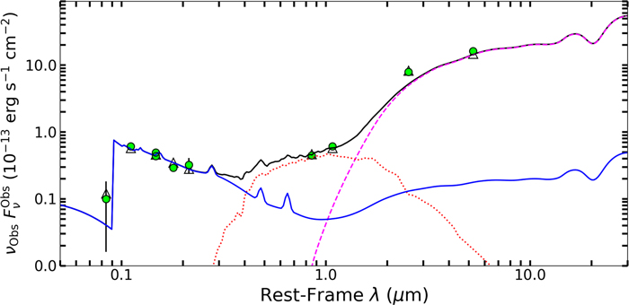
Figure 1. The SED of W0116–0505. The green circles show the observed fluxes in the SDSS  bands, the WISE W1–4 bands, and the SOAR r band presented by Assef et al. (2015). The solid black line shows the best-fit SED model, with the primary obscured AGN SED component shown by the dashed magenta line and the secondary unobscured AGN SED component shown by the solid blue line. The dotted red line shows the host galaxy component. The secondary AGN component most likely corresponds to scattered emission from the primary AGN component (see text for details).
Download figure:
Standard image High-resolution imageObject W0116–0505 was observed spectroscopically by the Sloan Digital Sky Survey (SDSS; Eisenstein et al. 2011). The spectrum, shown in part in Figure 2 (see Figure 2 of Assef et al. 2020, for the full spectrum), displays emission lines typically associated with quasars, supporting the scenario in which the blue-excess emission is due to scattered light from the obscured hyperluminous quasar (see Assef et al. 2020, for details). A closer look into some of the emission lines further reinforces this case. Specifically, by modeling the C iv emission line and the Si iv–O iv] blend with single Gaussian functions and a linear local continuum, as described in Assef et al. (2020), we find that their flux ratio of 2.9 ± 0.8 is consistent with the ratio of 2.8 found in the Vanden Berk et al. (2001) quasar composite. The equivalent width (EW) of the Si iv–O iv] of 32 ± 23 Å is not well constrained but is consistent with the value of 8.13 Å in the quasar composite. For C iv, on the other hand, we find a larger EW of 86 ± 17 Å compared with the 23.78 Å in the quasar composite, well in line with the mean of the distribution of C iv EWs found by Rakshit et al. (2020, see their Figure 13) for the SDSS DR14 quasar sample. We also model the Lyβ–O vi blend with two Gaussian functions, as well as the Lyα–N v with three Gaussian functions (as an extra narrow component seems to be needed for Lyα). We find that the combined flux ratio of Lyα–N v with respect to C iv of 4.38 ± 0.37 is consistent with that of 4.1 found in the Vanden Berk et al. (2001) composite. We find, however, that the Lyβ–O vi blend has a combined flux with respect to C iv of 1.56 ± 0.14, significantly in excess of the ratio of 0.38 found in the quasar composite. This may indicate specific properties of the Inter-Galactic Medium/Circum-Galactic Medium (IGM/CGM) around W0116–0505. A detailed characterization of the emission lines in Hot DOGs is being prepared by P. R. M. Eisenhardt et al. (2022, in preparation) and should help elucidate whether this is a common feature among these objects.
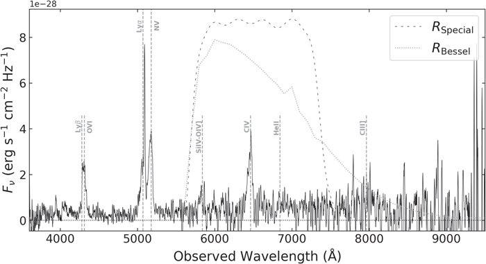
Figure 2. The SDSS spectrum of W0116–0505. The emission lines are marked with vertical gray dashed lines assuming a redshift of 3.173 (see Section 2.1 for details about the redshift). The plot also shows the response function of the FORS RSpecial (black dashed line) and RBessel (gray dotted line) filters.
Download figure:
Standard image High-resolution imageThe SDSS reported the redshift to be 3.1818 ± 0.0006. Wu et al. (2012), using a spectrum obtained at the MMT observatory, reported a slightly lower redshift of 3.173 ±0.001. A close inspection of the data shows that while the peak of the narrow component of the Lyα emission is consistent with the SDSS redshift, the O vi and the broad component of the Lyα emission line are consistent with that of Wu et al. (2012). Recently, Diaz-Santos et al. (2021) used a spectrum covering the CO(4–3) emission line obtained with the Atacama Large Millimeter/submillimeter Array (ALMA) to constrain the systemic redshift of W0116–0505 to 3.1904 ± 0.0002, implying a significant blueshift of the UV emission lines of 615 ± 45 and 1245 ± 73 km s−1, respectively, for the redshift estimates from SDSS and Wu et al. (2012). While a significant blueshift could be indicative of an ongoing merger, Assef et al. (2020) determined that the morphology of the W0116–0505 host galaxy in the Hubble Space Telescope (HST) WFC3 F160W band is consistent with an undisturbed early-type galaxy. This image, along with the HST/WFC3 F555W image presented by Assef et al. (2020), is shown in Figure 3. Note that, as discussed by Assef et al. (2020), the emission is resolved in both HST bands. We find that the source has half-light radii of 011 (0.9 kpc) and 0
23 (1.8 kpc) in the F555W and F160W bands, respectively. For reference, the point-spread functions (PSFs) in those bands, respectively, have FWHMs of 0
067 and 0
148.
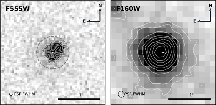
Figure 3. Cutouts (25 × 2
5) centered on W0116–0505 in the HST/WFC3 F555W (left) and F160W (right) bands. The white line in the center shows the orientation of the linear polarization measured in Section 3. The white contours show logarithmically spaced levels in relation to the brightest pixel, starting at 1%. The circles at the bottom left corner of each panel show the size of the PSF FWHM for each band. The gray dashed circle in the left panel is centered on W0116–0505 and has a physical radius of 3 kpc, as discussed in Section 4.4.
Download figure:
Standard image High-resolution image2.2. Imaging Polarimetry
Imaging polarimetric observations of W0116–0505 were obtained with the FORS2 instrument at the VLT using the RSpecial broadband filter (5710–7360 Å; see Figure 2). The observations were divided into four equal observing blocks (OBs), one executed on UT 2020-10-13, two on UT 2020-10-14, and one on UT 2020-10-15. Each OB consisted of 2 × 353 s observations of the target at retarder plate angles of 0°, 225, 45°, and 67
5, which are the recommended angles for linear polarization measurements in the FORS2 User Manual.
14
A zero-polarization standard star, WD 2039–202, and a polarization standard star, BD–12 5133, were observed with the same configuration on the night of UT 2020-10-12. Another zero-polarization standard, WD 0310–688, was observed with the same configuration on the night of UT 2020-09-25. Figure 4 shows an example of the images obtained for W0116–0505 on the first night of observations. Note that FORS2 simultaneously observes the ordinary (o) and extraordinary (e) beams for point sources (see González-Gaitán et al. 2020, as well as the FORS2 User Manual for further details). Because of this, the standard stars observed are not needed for calibration purposes to measure linear polarization but are still useful to check for the presence of systematic offsets. Table 1 summarizes the observations.
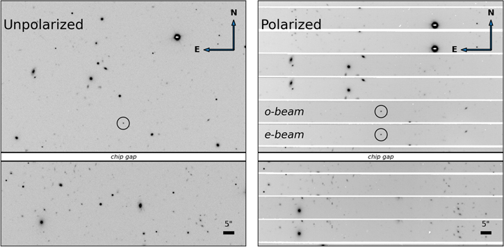
Figure 4. Cutouts (2′ × 2′) of the VLT/FORS2 images of W0116–0505 obtained on MJD 59,135. The left panel shows an image in the RSpecial band without the polarization optics, while the right panel shows a stack of all of the images obtained that night using the polarization optics. Note that a mask is used to separate the e and o beams, which alternate from top to bottom, allowing only 50% of the FoV to be observed at a time. The 3″ radius black circle shows the position of W0116–0505.
Download figure:
Standard image High-resolution imageTable 1. Summary of VLT/FORS2 Imaging Polarimetry Observations
| Target | Program ID | OB | Mean MJD | Airmass | Seeing |
|---|---|---|---|---|---|
| (days) | (arcsec) | ||||
| W0116–0505 | 106.218J.001 | 2886768 | 59,135.18 | 1.064 | 0.57 |
| 2886765 | 59,136.17 | 1.069 | 0.84 | ||
| 2886772 | 59,136.20 | 1.073 | 0.85 | ||
| 2886622 | 59,137.17 | 1.066 | 0.91 | ||
| Polarization Standard | |||||
| BD–12 5133 | 60.A-9203(E) | 200277970 | 59,133.98 | 1.117 | 1.19 |
| Zero-polarization Standards | |||||
| WD 0310–688 | 60.A-9203(E) | 200277988 | 59,117.36 | 1.410 | 1.58 |
| WD 2039–202 | 60.A-9203(E) | 200278006 | 59,134.00 | 1.003 | 0.70 |
Download table as: ASCIITypeset image
All images were bias subtracted using the EsoRex pipeline. 15 We did not apply a flat-field correction, as it is not recommended for linear polarization measurements (Aleksandar Cikota 2021, private communication), although we note that the results presented in the next section are not qualitatively changed if we apply one. We also did not apply a polarization flat-field correction, as none were available for dates close to those of our observations. González-Gaitán et al. (2020) found that the effects of applying this correction are negligible, so this should not affect our results. Finally, we remove cosmic rays in each frame using the algorithm of van Dokkum (2001) through the Astro-SCRAPPY tool (McCully et al. 2018).
3. Analysis
To estimate the linear degree of polarization of W0116–0505, as well as of the standard stars, we follow the procedure outlined in González-Gaitán et al. (2020) and the FORS2 User Manual. We first determine the Stokes Q and U parameters as

where θi
are the retarder plate angles of 0°, 225, 45°, and 67
5, and N = 4 is the total number of angles used. Here F(θi
) is defined as

where fo,i and fe,i are the summed instrumental o- and e-beam fluxes across all observations taken with retarder plate angle θi . Note that Q and U are already normalized by the Stokes parameter I. We use this notation throughout the article. To measure each flux, we perform aperture photometry using the Python package Photutils (Bradley et al. 2019). We use 2″ diameter apertures and estimate the background contribution using an annulus with inner and outer edge radii of 4″ and 7″, respectively. We note that using a smaller (larger) aperture diameter of 1″ (3″) nominally improves (worsens) the signal-to-noise ratio (S/N) of the detection, with only statistically consistent differences in the polarization amplitude and angle. However, since the observations of the final OB have seeing comparable to 1″, we conservatively chose to use the larger 2″ diameter aperture to minimize aperture losses between different plate angles due to seeing variations during those observations that could potentially induce systematic uncertainties in the Q and U parameter estimates. We analyze all OBs with the same aperture size for consistency.
For each source, we then remove the instrumental background polarization at its position within the field of view (FoV) using the corrections for Q and U provided by Equation (12) and Table 4 of González-Gaitán et al. (2020). These corrections are larger for objects toward the edges of the FoV but typically negligible near the center, where W0116–0505 and the standard stars were placed. Note that our conclusions are qualitatively unaffected if we do not apply these corrections.
We calculate the linear degree polarization p as

and the polarization angle χ as

Finally, we correct the angle χ for chromatism of the half-wave plate by subtracting the zero angle estimated for the R band of −119 in the FORS2 User Manual (see Table 4.7). Table 2 shows the linear polarizations and polarization angles measured for W0116–0505 and the standard stars.
Table 2. Linear Polarization Measurements
| Target | OB | P | χ |
|---|---|---|---|
| (%) | (deg) | ||
| W0116–0505 | 2886768 | 11.5 ± 3.5 | 72 ± 26 |
| 2886765 | 11.1 ± 3.7 | 75 ± 34 | |
| 2886772 | 10.2 ± 3.4 | 74 ± 35 | |
| 2886622 | 10.6 ± 4.1 | 77 ± 55 | |
| Combined | 10.8 ± 1.9 | 74 ± 9 | |
| Polarization Standard | |||
| BD–12 5133 | 200277970 | 4.12 ± 0.05 | 146.5 ± 0.3 |
| Zero-polarization Standards | |||
| WD 0310–688 | 200277988 | 0.04 ± 0.05 | ⋯ |
| WD 2039–202 | 200278006 | 0.12 ± 0.09 | ⋯ |
Download table as: ASCIITypeset image
To estimate the uncertainties in p and χ, we first estimate the nominal flux uncertainties for each measurement of fo,i and fe,i . Then, assuming the noise is Gaussian, we produce 1000 simulated values of fo,i and fe,i for each observation of each source and then combine them to form 1000 pairs of Q and U for each source. We then estimate the uncertainties in P and χ as the dispersion observed for the simulated pairs of Q and U.
For the zero-polarization standards, WD 0310–688 and WD 2039–202, we obtain linear polarizations of 0.04% ± 0.05% and 0.12% ± 0.09%. As expected, both are consistent with no polarization. For the polarization standard, BD–12 5133, we find a linear polarization of 4.12% ± 0.05% and a polarization angle of 1465 ± 0
3. These values are consistent at the 2σ level with the linear polarization fraction and angle of 4.02% ± 0.02% and 146
97 ± 0
13 measured by Fossati et al. (2007) using the FORS1 instrument and the RBessel band. The slightly higher polarization is likely due to the differences between the RSpecial filter used in our observations and the RBessel filter used by Fossati et al. (2007). Figure 2 shows the two filter curves.
16
Since RBessel extends somewhat redder than RSpecial and Fossati et al. (2007) measured a polarization that increases mildly toward 4.37% ± 0.05% at the V band, a slightly higher degree of polarization in the RSpecial band might be expected.
Following the procedure described above, we measure for W0116–0505 a polarization of 10.8% ± 1.9% and a polarization angle of 74°± 9° when combining the observations of all four OBs. If we instead analyze the observations separately for each OB, we find consistent values for both the polarization fraction and angle, albeit with larger uncertainties, as shown in Table 2. This shows that the high linear polarization detected for W0116–0505 is not driven by outliers in the observations. As a further check, we follow the procedure above to estimate the linear polarization for all objects in the FoV of W0116–0505 detected with S/N ≥ 5 in the e beam of a single exposure that were not affected by obvious issues such as artifacts and blending with neighboring sources. Figure 5 shows the linear polarizations detected and their uncertainties for all of these sources, and W0116–0505 is the only source that has a detection above 3σ. This confirms that the measurement is not driven by a problem with data reduction or the analysis procedures. Furthermore, it shows that the detected polarization is not caused by interstellar gas and dust. As a further check to constrain the effects of interstellar polarization, we take all 55 stars in the catalog of Heiles (2000) of stellar polarizations that are within 10° of W0116–0505 and combine their polarization signals by adding their Q and U Stokes parameters, assuming the same value of I. As their intrinsic polarization will have random orientations, the only coherent term that should survive the averaging is that caused by the interstellar medium (ISM). This estimate yields pinterstellar = 0.064%, well below the linear polarization fraction detected for W0116–0505. In the next section, we discuss the implication of this high degree of polarization detected for W0116–0505.
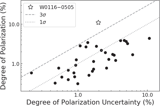
Figure 5. Degree of polarization and its uncertainty for W0116–0505 compared to that of all other targets detected with S/N > 5 e-beam fluxes in single observations without obvious systematic problems. The diagonal gray lines show linear polarizations detected at 1σ (dotted) and 3σ (dashed). Object W0116–0505 is the only source in the field with a linear polarization detection of >3σ.
Download figure:
Standard image High-resolution image4. Discussion
4.1. The Case for Scattered Light in BHDs
As discussed in Section 1, Assef et al. (2016) identified a group of eight BHDs by studying the SEDs of a sample of Hot DOGs. When accounting for selection biases, Assef et al. (2016) found that up to 12% of Hot DOGs could be classified as BHDs, although they suggested that the true fraction is likely lower. Considering the results of their SED modeling, Assef et al. (2016) determined three possible sources of the blue-excess emission of BHDs: (a) a secondary AGN in the system, (b) a luminous unobscured starburst outside the range of the templates of Assef et al. (2010), and (c) scattered light from the highly obscured central engine.
Assef et al. (2016, 2020) conducted detailed studies using HST/WFC3 and Chandra/ACIS observations, as well as ground-based photometry and spectroscopy of three BHDs, W0204–0506, W0220+0137, and W0116–0505 (the subject of the present polarimetry study), in the context of each hypothesis. Based on the lack of soft X-ray emission detected in all three sources and the centrally concentrated undisturbed morphologies of W0220+0137 and W0116–0505, the presence of an additional unobscured AGN in the system (hypothesis (a)) was judged to be highly unlikely. They also determined that an unobscured starburst (hypothesis (b)) was unlikely to be the dominant source of the rest-frame UV/optical emission due to the high star formation rates required but could not rule this out completely (see Assef et al. 2020 for details). For W0204–0506, Assef et al. (2020) pointed out that the disturbed morphology with some significantly extended UV flux implied that star formation could account for a fraction of the observed blue-light excess. Both studies, based on the challenges of the other scenarios, concluded that the most likely source of the excess blue-light emission is scattered emission from the highly obscured central engine (hypothesis (c)).
Further insights can be obtained by analyzing the variability of the UV continuum, as no significant variability would be expected for an unobscured starburst. For W0116–0505, we can compare the r-band fluxes of SDSS and PanSTARRS PS1 to cover a significantly long timescale, particularly since there are almost no color effects between the surveys in this band (Tonry et al. 2012). We find that the PSF-fitting magnitudes are fainter by about 0.14 ± 0.06 mag in the PS1 DR2 mean object catalog as compared to SDSS DR16. The PS1 observations were obtained between 60 and 513 rest-frame days after the SDSS observations. Variability supports hypotheses (a) and (c), in which the rest-frame UV flux is dominated by AGN emission. This amplitude, while small, is somewhat above what would be expected for a luminous AGN in such a timescale (e.g., Vanden Berk et al. 2004; MacLeod et al. 2010), and it could be due to a systematic difference between the PS1 and SDSS photometry of the source. A deeper analysis, beyond the scope of this study, would be needed to address systematic uncertainties.
As discussed in Section 1, polarization can be a powerful tool to confirm that the source of the blue excess is indeed scattered AGN light, as we would not expect significant linear polarization from star formation. The linear polarization of p = 10.8% ± 1.9% found for W0116–0505 in the RSpecial band in Section 3 shows that the UV emission is dominated by scattered emission from the central engine rather than star formation, confirming the conclusions of Assef et al. (2020) for this source. In the following sections, we discuss the effects that differing polarization between the UV continuum and the broad emission lines could have on our broadband polarization measurement, as well as the implications for obscuration geometry and the properties of the scattering medium in W0116–0505.
4.2. Polarized Light of Continuum versus Emission Lines
The broad emission lines could, in principle, show different linear polarization properties from the continuum as they arise from physically distinct structures, namely, the broad-line region and the accretion disk. As discussed in Assef et al. (2020), W0220+0137 is classified as an extremely red quasar (ERQ), and W0116–0505 is classified as ERQ-like (see Hamann et al. 2017; Goulding et al. 2018). Alexandroff et al. (2018) found for three objects, an ERQ, an ERQ-like, and a type 2 quasar, a 90° difference between the polarization angle of the Lyα, N v, and C iv broad emission lines in certain velocity ranges and the continuum emission, with a linear degree of polarization of ∼10% in the continuum and ∼5% in the emission lines. Our broad band encompasses both the UV continuum and the C iv broad emission line, which has an EW of 86 ± 17 Å. Hence, the linear degree of polarization of the continuum alone and/or the C iv line may separately exceed the 10.8% ± 1.9% determined in Section 3. If we assume that both the continuum and the emission line fluxes have the same degree of polarization, pint, but with polarization angles differing by 90°, the measured p relates to pint by

where fc and fl are the fraction of the integrated flux in the RSpecial band coming from the continuum and emission line, respectively. Modeling the continuum as a linear function of the wavelength and emission line as a single Gaussian, as outlined in Assef et al. (2020), we find that 82% of the flux in the RSpecial band is contributed by the continuum, implying pint = 17%. Future spectropolarimetric or imaging polarimetry observations in multiple broad bands could further elucidate this point. We direct the reader to Alexandroff et al. (2018) for a more comprehensive overview of possible geometries that can potentially explain the high degree of polarization and a swing in the polarization angle between the continuum and the broad emission lines.
4.3. The Scattering Medium of W0116–0505
Assef et al. (2020) argued that if the UV was dominated by scattered light, the scattering medium was more likely ionized gas rather than dust, as there was no significant “bluening” of the underlying AGN spectrum according to the AGN template of Assef et al. (2010). However, they could not discard dust as the scattering medium, as there were too few photometric data points to rule out the possibility of ISM dust reddening canceling the bluening of the input spectrum. Furthermore, for some types of dust, no bluening may be observed. For example, Zubko & Laor (2000) showed that for the type of dust proposed by Mathis et al. (1977), no bluening is observed at λ ≲ 2500 Å for scattering angles ≳30°.
In order to analyze the properties of the scattering medium, we consider the degree of polarization detected and the total scattered flux in the context of a simple model, similar to that explored by Miller et al. (1991). Furthermore, we take into consideration the fact that the scattered continuum is unreddened and the UV continuum is resolved in the HST/WFC3 F555W images (see Assef et al. 2020, and discussion below for details). To construct the model, we first assume that the scattering medium is optically thin to the scattered radiation. In other words, we assume that the UV photons reaching us have only experienced a single scattering event along their path. We also assume that the accretion disk is covered by a traditional torus with two polar openings, each of angular half-size ψ, through which UV light can escape and interact with the scattering medium. We study the geometry of the system in spherical coordinates with the polar axis pointing at our line of sight, as shown in Figure 6. In these coordinates, r corresponds to the distance of a scattering particle from the supermassive black hole. Conveniently, the scattering angle of that scattered radiation corresponds to the particle’s polar angle, so we refer to both as θ in this section. The polarization angle of the radiation scattered by that particle, χparticle, is conveniently related to its azimuthal angle ϕ by χparticle =ϕ + π/2. In this model, the centers of the openings in the torus are respectively inclined by polar angles θ = η and ηS + π from the line of sight.
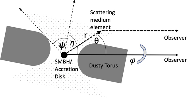
Figure 6. Schematic drawing of the geometry for the optically thin scattering model discussed in Section 4.3.
Download figure:
Standard image High-resolution imageIn general, we can say that the total flux from the AGN accretion disk scattered into our line of sight is given by

where FAD is the flux we would receive if we had an unobscured line of sight to the accretion disk,  is the differential scattering cross section per hydrogen nucleon for scattering angle θ, and nH is the number density of hydrogen atoms. The integral is carried over the volume of all regions of the galaxy illuminated by the AGN through the openings in the torus. We further assume that nH is only a function of r and note that the column density NH is given by

Equation (6) can be rewritten to depend on the fraction of the accretion disk flux scattered into our line of sight, fScatt = FScatt/FAD. However, we do not have a direct measurement of FAD, as we can only probe the brightness of the torus from the IR emission due to the dust obscuration. The relation between the accretion disk luminosity and the torus luminosity is given by the covering factor of the torus, which, for our model of a torus with two polar openings of angular half-size ψ, is given by  . In other words,

Assef et al. (2020) found that the AGN that reproduced the scattered component in the UV and optical had = 0.6% of the luminosity of the obscured AGN that reproduced the mid-IR component when both components were modeled with the same AGN template from Assef et al. (2010; see Figure 1). We assume that the coverage fraction for the Assef et al. (2010) empirical AGN SED template used is half, since Assef et al. (2013) found that, on average, ∼50% of quasars appeared obscured in a sample similar to that used by Assef et al. (2010) to define their template. We also note that Roseboom et al. (2013) found a dust covering fraction of ∼40% for quasars in a slightly higher luminosity range than those used by Assef et al. (2010). Considering this in conjunction with Equation (8), we find that

Using Equations (7) and (9), we can rewrite Equation (6) as

where NH is the hydrogen column density and

We note that while Equation (8) could potentially be used to constrain the maximum size of ψ so as to avoid an accretion disk luminosity that would exceed the most luminous type 1 quasars known (e.g., Schindler et al. 2019), these constraints are weaker than the ones discussed below.
Using the same assumptions and geometry, we also calculate the total degree of polarization and polarization angle by noting that the Stokes parameters Q and U are additive. Furthermore, we orient the zero-point of the azimuthal axis such that the torus openings are found along ϕ = 0, π, which is equivalent to saying that the overall polarization angle of the system will be π/2. In this case, U is always equal to zero, and the degree of polarization is given by p = −Q. We can rewrite the latter expression as

where

and pparticle(θ) is the polarization degree caused by the scattering particle when irradiated by unpolarized light. We note that by dividing Equations (10) and (12), we can write the overall degree of polarization as

4.3.1. Thomson Scattering
First, let us consider the simplest scenario, where the scattering medium is purely composed of ionized hydrogen. In this case, we have simple Thomson scattering due to free electrons, with the density of the free electrons being the same as the density of the hydrogen nucleons. The differential cross section per hydrogen nucleon is then given by

where r0 is the classical electron radius, and the polarization degree per particle is given by

The top left panel of Figure 7 shows the degree of polarization as a function of ψ and η. The minimum inclination angle for the openings is  , as lower inclination angles cannot reproduce the observed degree of polarization of p = 10.8%. At that inclination angle, ψ would have to be close to zero in order to not depolarize the combined emission. As η becomes larger, ψ becomes larger as well in order to depolarize the combined emission and bring it down to the observed value. When the opening is inclined perpendicular to the line of sight (i.e., the torus is edge-on), it reaches its maximum possible size of
  .
.
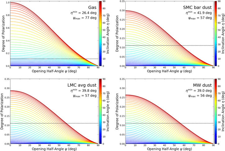
Figure 7. Degree of polarization expected as a function of opening angle ψ and inclination angle η of the dust torus for the model discussed in Section 4.3 for purely ionized gas (top left), the SMC bar dust mixture (top right), the LMC average dust mixture (bottom left), and the MW dust mixture (bottom right) of Draine (2003). The inclination angle η is indicated by the line color and the color bar on the right. The horizontal dashed line shows the measured polarization fraction for W0116–0505.
Download figure:
Standard image High-resolution imageIn addition to analyzing the degree of polarization expected for a given geometry, we can also use Equations (10) and (12) to find for each value of η the values of ψ and NH that simultaneously reproduce the observed degree of polarization and the fraction of the incident flux scattered into our line of sight. Figure 8 shows the required value of NH as a function of ψ and η. For all geometries, we would require column densities of NH > 5 × 1021 cm−2. The much larger values required for low inclination angles and small torus openings potentially conflict with the model assumption of an optically thin medium from the line of sight of the observer. If we consider that multiply scattered photons lose the ensemble polarization properties, then an optically thick medium would require a larger minimum inclination angle in order to reproduce the observed degree of polarization.
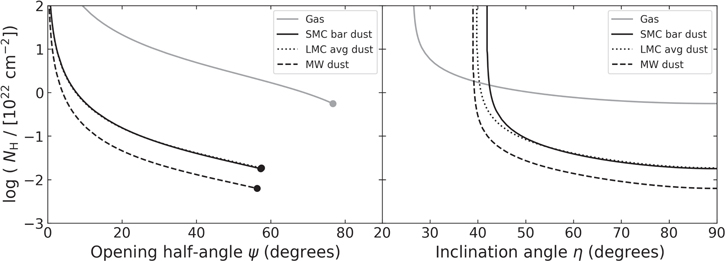
Figure 8. Constraints on the scattering medium NH as a function of the opening angle ψ (left) and inclination angle η (right) of the dust torus for the model discussed in Section 4.3. Note that in the left panel, the lines from the SMC bar and LMC average dust mixtures almost completely overlap.
Download figure:
Standard image High-resolution imageSince dust particles have a much larger scattering cross section than free electrons, their contribution to scattering can easily dominate over that of Thomson scattering off free electrons. Draine (2003) conducted a detailed study of the scattering properties of UV and optical light for different dust-to-gas mixtures and found the dust differential scattering cross section per hydrogen nucleon in the UV for the type of dusty ISM typically found in the SMC, Large Magellanic Cloud (LMC), and MW to be between ∼5 × 10⁻²⁴ and ∼10−21 cm2 H−1 sr−1, depending on the exact dust mixture and scattering angle. In a fully ionized hydrogen medium, the differential scattering cross section per hydrogen nucleon would be of order  . Hence, dust scattering from the former should dominate over free electrons unless the scattering medium is very dust-deficient. We expect dust to be present in significant quantities in the ISM of the host galaxy as, by selection, Hot DOGs have bright dust emission in the mid-IR and are typically well detected in the far-IR (Jones et al. 2014; Wu et al. 2014; Diaz-Santos et al. 2021).
17
Hence, the Thomson scattering scenario would only be plausible if the scattering medium is within the dust sublimation radius of the accretion disk, which we estimate to be 8.7 pc using Equation (1) of Nenkova et al. (2008) and the bolometric luminosity of W0116–0505 measured by Tsai et al. (2015), adjusted for the differences in the cosmological model assumed. In order to have a direct line of sight toward the inner regions of the torus but without a direct line of sight to the accretion disk, we need ψ ∼ η, which is achieved at two different inclination angles of η ≈ 28° and ≈76°, as shown in Figure 9.
. Hence, dust scattering from the former should dominate over free electrons unless the scattering medium is very dust-deficient. We expect dust to be present in significant quantities in the ISM of the host galaxy as, by selection, Hot DOGs have bright dust emission in the mid-IR and are typically well detected in the far-IR (Jones et al. 2014; Wu et al. 2014; Diaz-Santos et al. 2021).
17
Hence, the Thomson scattering scenario would only be plausible if the scattering medium is within the dust sublimation radius of the accretion disk, which we estimate to be 8.7 pc using Equation (1) of Nenkova et al. (2008) and the bolometric luminosity of W0116–0505 measured by Tsai et al. (2015), adjusted for the differences in the cosmological model assumed. In order to have a direct line of sight toward the inner regions of the torus but without a direct line of sight to the accretion disk, we need ψ ∼ η, which is achieved at two different inclination angles of η ≈ 28° and ≈76°, as shown in Figure 9.
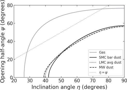
Figure 9. Opening angle ψ as a function of the inclination angle η of the dust torus for the model discussed in Section 4.3. Line styles have the same meaning as in Figure 8.
Download figure:
Standard image High-resolution imageThe extension of the UV emission in the HST/F555W image, which has a half-light radius of 0.9 kpc, as mentioned in Section 2.1, is also hard to reconcile with the idea of the scattering occurring within the sublimation radius, which is 2 orders of magnitude smaller. The UV emission in extended scales would either require substantial scattering by the ISM, which is likely dominated by dust, or a significant star formation component, which was deemed unlikely by Assef et al. (2020). Furthermore, the host galaxy emission is more extended in a direction that is close to perpendicular to the polarization angle, as shown in Figure 3, suggesting that this extended component is along the regions illuminated by AGN and consistent with being scattered light.
Considering all of this, we conclude that it is unlikely that Thomson scattering can be the dominant scattering mechanism in W0116–0505, so substantial dust scattering is very likely. We now look at optically thin dust in the ISM as the possible scattering medium.
4.3.2. Scattering by Optically Thin Dust
We conduct the same analysis done for Thomson scattering but using the differential cross section per hydrogen nucleon and degree of polarization provided by Draine (2003) for an RV = 3.1 MW dust mixture, as well for the dust mixtures for the SMC bar and LMC average of Weingartner & Draine (2001).
18
Specifically, we use those determined for a rest-frame wavelength of 1600 Å, which is close to the rest-frame wavelength that corresponds to the effective wavelength of the RSpecial filter. Figure 7 shows the expected observed polarization for these dust mixtures as a function of η and ψ. The SMC bar dust mixture provides the highest possible linear polarization, but all three are easily capable of reproducing the observed value, with minimum inclination angles of  , 39
, 398, and 39
0 for the SMC, LMC, and MW dust mixtures, respectively. At an inclination of 90°, the opening must again be maximal to allow for enough depolarization to match the observed degree of polarization. The maximum openings are somewhat smaller than for the Thomson scattering case, with
 , 57°, and 56° for the three dust mixtures. Figure 8 shows the required values of NH as a function of ψ and η to reproduce the observations. We find that the values are very similar for the SMC and LMC dust mixtures, both requiring NH > 1.8 × 1020 cm−2, while the MW dust mixture only requires NH > 6 × 1019 cm−2.
The hydrogen column densities expected in the case of optically thin dust mixtures are consistent with the lack of reddening found by Assef et al. (2020) for the scattered light (E(B − V) < 0.02 mag, 1σ limit). Maiolino et al. (2001) studied the dust-to-gas ratio in the circumnuclear regions of nearby AGN and found ratios that were significantly below the Galactic standard value of AV /NH = 4.5 × 10⁻²² mag cm2 (Güver & Özel 2009), or E(B − V)/NH = 1.5 × 10⁻²² mag cm2 assuming RV = 3.1. Maiolino et al. (2001) found a median ratio in nearby AGN of E(B − V)/NH = 1.5 × 10⁻²³ mag cm2, about 10 times lower than the Galactic standard, albeit with a large variance. A reddening of E(B − V) < 0.02 mag would then require NH < 1.3 × 1021 cm−2 for the Maiolino et al. (2001) median value, which is consistent with the results of our simple model for η ≳ 40°–50° and ψ ≳ 10°–25°, depending on the exact dust mixture. For the Galactic standard value, we would instead need NH < 1.3 × 1020 cm−2, which is only achievable for the MW dust mixture for η ≳ 60° and ψ ≳ 40°.
A more complex model could consider multiple additional openings in the torus through which the light from the central engine is escaping into the ISM. In the case of multiple openings in the dust distribution, each will create linearly polarized emission but with different polarization degrees and angles, resulting in dilution of the combined linear polarization. Such a scenario would require a higher inclination of the main openings through which the light is escaping in order to achieve the same overall polarization of 10.8%. A contribution from star formation would also have the effect of diluting the linear polarization signal, although Assef et al. (2020) found it unlikely that there is a significant contribution from star formation to the UV/optical SED of W0116–0505, as mentioned earlier.
4.4. Outflow in W0116–0505 as a Possible Scattering Medium
In the previous section, we analyzed the observed degree of polarization in W0116–0505 in the context of a simple model in which an AGN is surrounded by a torus with bipolar openings through which light can escape and interact with a uniform ISM. We showed that for reasonable dust mixtures, the model is able to reproduce three key aspects of our observations, namely, a degree of polarization of 10.8%, a fraction of the total flux scattered into our line of sight of 0.6%, and a scattered flux consistent with no dust reddening. While the model is quite simple and depends only on three parameters (NH, ψ, and η), the parameters are heavily degenerate, suggesting that a more complicated model is not warranted without further constraints.
While the observations are consistent with a regular ISM being the source of the scattering, this is clearly not a unique scenario. In particular, the more sophisticated model proposed by Alexandroff et al. (2018) should be able to explain the observations as well, as the objects analyzed in that work share a number of similarities with W0116–0505. In that model, the scattering medium consists of a fast outflow escaping through a polar opening in the AGN torus. Here we consider as well the possibility of an outflow being responsible for the scattered light, but with a different approach. Finnerty et al. (2020) found that the AGN in W0116–0505 is driving a massive gas outflow with an estimated total mass of Mgas = 1.6 × 10⁹ M⊙, based on the width and luminosity of its very broad and blueshifted [O iii] emission lines. The luminous [O iii] emission implies that this outflow is necessarily being illuminated by the AGN, suggesting that the outflow could also play a role in the scattering.
We can make a rough estimate of the hydrogen column density in the outflow by noting that NH ≥ 〈nH〉Rout for radially declining density profiles such as an isothermal sphere, with the equality corresponding to the limit case of a uniform gas distribution. We take the mean electron density of 〈ne 〉 =300 cm−3 and outflow extension of Rout = 3 kpc assumed by Finnerty et al. (2020) and assume that the outflow is primarily composed of ionized hydrogen and helium with the helium number density being 10% of that of hydrogen (as in Carniani et al. 2015), implying that 〈ne 〉 = 〈nH〉/1.2. With these assumptions, we estimate NH ≥ 2.3 × 1024 cm−2, implying a Compton-thick outflow. Using the Maiolino et al. (2001) median dust-to-gas ratio, this column density would translate to a reddening of E(B − V) ≥ 35 mag, although it is important to note that this value is of limited accuracy given the substantial uncertainties in the assumed values of 〈ne 〉 and Rout as discussed by Jun et al. (2020), as well as in the assumed dust-to-gas ratio.
In a more physically motivated picture, it might be possible that the AGN in W0116–0505 is launching polar, possibly dusty outflows, as is commonly seen in nearby counterparts, albeit at much lower luminosities and outflow masses (e.g., Schlesinger et al. 2009; Rupke et al. 2017; Stalevski et al. 2017; Alonso-Herrero et al. 2021), which by themselves might be responsible for the openings in the dust torus. Figure 10 shows a schematic drawing of this scenario. Assuming that the outflow is biconical with an opening half-angle ψ and hence spread over the entirety of the regions illuminated by the accretion disk through the torus openings, a more conservative estimate of the column density can be achieved by using the luminosity of the [O iii] outflow measured by Finnerty et al. (2020) of ![$\mathrm{log}{L}_{[O{\rm\small{III}}]}/{L}_{\odot }=11.5$](https://content.cld.iop.org/journals/0004-637X/934/2/101/revision1/apjac77fcieqn12.gif) . It can be shown that the mean electron density in this case would be given by
. It can be shown that the mean electron density in this case would be given by
where f is the filling factor of the outflow. We have made the same assumptions of Jun et al. (2020) and Finnerty et al. (2020) that ![$\langle {n}_{e}{\rangle }^{2}/\langle {n}_{e}^{2}\rangle \approx {10}^{[{\rm{O}}/{\rm{H}}]}$](https://content.cld.iop.org/journals/0004-637X/934/2/101/revision1/apjac77fcieqn13.gif) (or, equivalently, that the metallicity is solar and
(or, equivalently, that the metallicity is solar and  ), the electron temperature is ≈10,000 K, and the gas has the same hydrogen and helium composition as before (see also Carniani et al. 2015). We note that for that electron temperature, the [O iii] emissivity is relatively insensitive to the electron density, showing a variation of less than 3% between ne
= 1 and 10,000 cm−3 according to the software PyNeb (Luridiana et al. 2015), so we have assumed the same value used by Carniani et al. (2015) of 3.4 × 10⁻²¹ erg s−1 cm3 for consistency. Following the same argument as in the previous paragraph to estimate a lower bound on the column density based on the mean electron density, we find that
), the electron temperature is ≈10,000 K, and the gas has the same hydrogen and helium composition as before (see also Carniani et al. 2015). We note that for that electron temperature, the [O iii] emissivity is relatively insensitive to the electron density, showing a variation of less than 3% between ne
= 1 and 10,000 cm−3 according to the software PyNeb (Luridiana et al. 2015), so we have assumed the same value used by Carniani et al. (2015) of 3.4 × 10⁻²¹ erg s−1 cm3 for consistency. Following the same argument as in the previous paragraph to estimate a lower bound on the column density based on the mean electron density, we find that  . Using the median gas-to-dust ratio of Maiolino et al. (2001), we find E(B − V) ≥ 1.5 mag for the largest possible value of ψ = π/2, which would still imply an obscured view to the accretion disk through the outflow. We note that the electron densities implied by Equation (17) for ψ ≳ 5° and f ∼ 1 are well below the typical values of ∼500 cm−3 found by, e.g., Karouzos et al. (2016) in AGN outflows and well below the estimates of Jun et al. (2020) of 〈ne
〉 ∼ 1100 and 600 cm−3 for outflows in two Hot DOGs using the [S ii] doublet. This implies that either the opening angle is small, making the outflow typical dust reddening much larger than 1.5 mag for lines of sight through the outflow, or the outflow has a low filling factor, in which case obscuration might vary significantly for different lines of sight. A low filling factor might indeed be necessary to explain the high observed L[O III], although we cannot disregard the possibility that the intrinsic L[O III] could be larger due to obscuration. Combined with the uncertainties inherent to some of the assumptions made (as discussed in the previous paragraph), quantitative predictions are inaccurate. However, given the analysis presented here, we can qualitatively conclude that the outflow is likely optically thick at UV and optical wavelengths for most lines of sight.
. Using the median gas-to-dust ratio of Maiolino et al. (2001), we find E(B − V) ≥ 1.5 mag for the largest possible value of ψ = π/2, which would still imply an obscured view to the accretion disk through the outflow. We note that the electron densities implied by Equation (17) for ψ ≳ 5° and f ∼ 1 are well below the typical values of ∼500 cm−3 found by, e.g., Karouzos et al. (2016) in AGN outflows and well below the estimates of Jun et al. (2020) of 〈ne
〉 ∼ 1100 and 600 cm−3 for outflows in two Hot DOGs using the [S ii] doublet. This implies that either the opening angle is small, making the outflow typical dust reddening much larger than 1.5 mag for lines of sight through the outflow, or the outflow has a low filling factor, in which case obscuration might vary significantly for different lines of sight. A low filling factor might indeed be necessary to explain the high observed L[O III], although we cannot disregard the possibility that the intrinsic L[O III] could be larger due to obscuration. Combined with the uncertainties inherent to some of the assumptions made (as discussed in the previous paragraph), quantitative predictions are inaccurate. However, given the analysis presented here, we can qualitatively conclude that the outflow is likely optically thick at UV and optical wavelengths for most lines of sight.
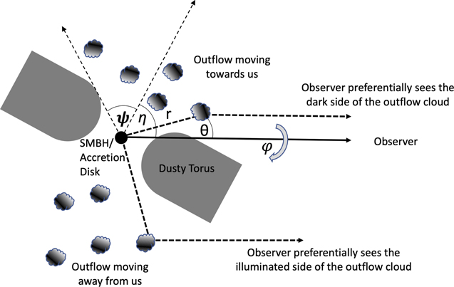
Figure 10. Schematic drawing of the geometry for the optically thick outflow scattering model discussed in Section 4.4.
Download figure:
Standard image High-resolution imageZubko & Laor (2000) studied the polarization due to scattering by dust grains and showed that the degree of polarization from an optically thick dust sphere is almost unchanged from that of optically thin dust (see their Figure 17). They also showed that at a rest-frame wavelength of 1600 Å, the fraction of the scattered flux for an optically thick dust sphere rises with the scattering angle (see their Figure 16) and is maximum at θ = 180°, when our line of sight looks directly at the illuminated side of the sphere (i.e., backscattering). Considering this, we propose the following scenario. We assume that the AGN in W0116–0505 is launching a biconical outflow. We also assume that the biconical outflow has an  consistent with the lower limits estimated above, and that the ISM outside of the outflow has a much lower column density. We propose, then, that the scattered flux we observe comes from backscattered light on the surface, primarily at the base, of the receding outflow. Scattered light from the inner regions of the outflow is not dominant at 1600 Å due to both dust reddening and multiple scattering events diluting the signal, although we note that the dust in the outflows cannot be too optically thick far from the base in order to permit us observing the blueshifted [O iii] emission from the approaching outflow that is very prominent in the spectrum of W0116–0505 (see Finnerty et al. 2020).
This potential scenario has the interesting property that even for the lines of sight that go through the torus openings, W0116–0505 would likely be observed as a highly obscured quasar or, more specifically, a Hot DOG. In the next section, we speculate how BHDs might be related to other populations of obscured hyperluminous quasars in the literature.
4.5. A Potential Relation between BHDs, ERQs, and Heavily Reddened Type 1 Quasars
In Section 4.4, we proposed that the blue excess in W0116–0505 might be caused by accretion disk light scattered by the massive ionized gas outflow known in the system. We also found that, in this scenario, an observer looking through the approaching outflow, and hence through the opening in the torus, would likely still observe an obscured quasar due to the optical thickness of the outflow. Specifically, we estimated that, in the best of conditions, a typical line of sight through the outflow would observe the central engine with a reddening of E(B − V) ≥ 1.5 mag (although with considerable uncertainty). As the outflow expands, however, the column density will decrease, eventually allowing a significant number of lines of sight with a direct view to the accretion disk. Recently, Banerji et al. (2015) presented a population of hyperluminous heavily reddened type 1 quasars at z > 2 with 0.5 ≲ E(B − V) ≲ 1.5. We speculate that, if the scenario in W0116–0505 of a biconical outflow is correct, W0116–0505 could potentially be a precursor to these heavily reddened type 1 quasars. Recently, Temple et al. (2019) showed that heavily reddened type 1 quasars also have fast ionized gas outflows. None of the objects they studied, however, had as high a velocity dispersion as the FWHM 4200 ± 100 km s−1 found in W0116–0505 by Finnerty et al. (2020), and all objects in Temple et al. (2019) had lower [O iii] luminosities by 1–2 orders of magnitude compared to W0116–0505, suggesting the outflowing gas is more diffuse. Lansbury et al. (2020) found that the hydrogen column densities obscuring the X-rays in heavily reddened type 1 quasar are in the range of 1–8 × 1022 cm−2, considerably below the nearly Compton-thick obscuration of Hot DOGs and BHDs (Stern et al. 2014; Piconcelli et al. 2015; Assef et al. 2016, 2020; Vito et al. 2018). This might be consistent with W0116–0505 tracing an earlier evolutionary stage than heavily reddened type 1 quasars.
We further speculate that this source of the blue excess may extend to all or most BHDs. In particular, we note that Finnerty et al. (2020) found outflow properties similar to W0116–0505 for W0220+0137. As for W0116–0505, Assef et al. (2020) concluded that the most likely source for the UV emission is scattered emission from the central engine for W0220+0137, suggesting that polarimetric observations should also identify a significant degree of linear polarization. As mentioned earlier, both targets are also classified as ERQs, and a spectropolarimetric study of ERQs by Alexandroff et al. (2018) identified a significant degree of polarization in their UV light. Furthermore, Zakamska et al. (2016) identified significant ionized gas outflows in some ERQs, similar to those found by Finnerty et al. (2020) for W0116–0505 and W0220+0137. Hence, ERQs may be closely related to BHDs, and both may relate to heavily reddened type 1 hyperluminous quasars.
We suggest that Hot DOGs, ERQs, and heavily reddened type 1 quasars are related to each other through both evolution and line-of-sight obscuration. Specifically, we hypothesize that Hot DOGs represent the earliest stage of these hyperluminous objects, with the central engine completely enshrouded in dust. With no light escaping from the central engine into the ISM, their UV emission is dominated by starlight from the host galaxy (see Wu et al. 2012; Assef et al. 2015), leading to relatively faint observed-frame optical fluxes. At some point in their evolution, these objects start driving massive, fast outflows, leading to the formation of large openings in their dust torus. In the early stages of this outflow phase, the objects are observed as BHDs/ERQs when observed along lines of sight that allow a view to the receding outflow and hence maximize the scattered flux. In the later stages of this outflow phase, once the outflow has expanded and hence lowered its column density, an observer looking through the outflow would see the object as a heavily reddened type 1 hyperluminous quasar. The picture we have outlined here is qualitatively similar to that suggested by, e.g., Hopkins et al. (2008), so we can also hypothesize that once the outflowing material is cleared out of the ISM, these objects will transition to regular type 1 quasars with no obscuration when observed through the openings in the dust torus. A similar scenario was recently suggested by Lansbury et al. (2020) and Jun et al. (2021) based on estimates of the radiation feedback in luminous obscured quasars. Recently, Diaz-Santos et al. (2021) suggested that the availability of gas at large scales may lead to Hot DOGs being a recurring phase throughout the evolution of massive galaxies, with each episode perhaps leading to a BHD/ERQ/heavily reddened type 1 quasar phase as well, while the massive outflows slowly deplete the gas available in the ISM of their host galaxies.
Further polarimetric observations of more BHDs and ERQs will be needed to better constrain models for the light scattering and enable stronger connections to be drawn between these populations. Ovservations with the JWST/NIRSPEC IFU may be able to determine the size and profile of the outflow in W0116–0505, as well as in other BHDs, ERQs, Hot DOGs, and heavily reddened type 1 quasars. Additional constraints on the relationship between these populations may come from the studies of their environments, as those would remain stable through these relatively fast transitions.
5. Conclusions
We have presented imaging polarimetry observations in the RSpecial broad band using the VLT/FORS2 instrument of W0116–0505 at z = 3.173, identified by Assef et al. (2020) as a BHD. We measure a linear polarization of p = 10.8% ± 1.9% with a polarization angle of χ = 74° ± 9°. This high degree of polarization confirms the scattered-light scenario and effectively discards an extreme, unobscured starburst as the primary source of the observed excess UV emission in W0116–0505.
We discuss the implications for the dust obscuration geometry and the properties of the scattering medium in the context of a simple model in which the central engine is covered by a dust torus with two polar openings through which light can escape and illuminate an ISM that is optically thin for scattered light. For this model, we find that both Thomson scattering and optically thin dust scattering can reproduce the observed linear polarization and total scattered flux for a wide range of ISM column densities and torus geometries. Optically thin dust scattering is much more likely than Thomson scattering because a dust-free scattering medium would only be expected within the dust sublimation radius of the AGN.
However, this is not a unique scenario, and we also discuss the possibility that the scattering medium is a biconical dusty outflow aligned with the torus openings. In this scenario, the scattered flux might be dominated by light backscattered off the base of the outflow receding from us. In this scenario, once the outflow expands, observers with a direct line of sight to the accretion disk through the dusty outflow might see a reddened AGN, possibly consistent with the heavily reddened type 1 hyperluminous quasars identified by Banerji et al. (2015). We hypothesize that BHDs are closely related to ERQs and may correspond to the same objects identified by Banerji et al. (2015) at a slightly earlier evolutionary stage. We speculate that there could be an evolutionary sequence in which BHDs/ERQs/heavily reddened type 1 hyperluminous quasars are the intermediate stage between Hot DOGs without blue excess and traditional type 1 quasars of similar luminosities.
We thank Aleksandar Cikota for helping us with the reduction of the FORS2 imaging polarimetry data and Matthew Temple and Aaron Barth for comments and suggestions that helped improve our work. We also thank the anonymous referee for all of the comments and suggestions on the submitted manuscript. R.J.A. was supported by FONDECYT grant No. 1191124 and ANID BASAL project FB210003. F.E.B. acknowledges support from ANID-Chile BASAL AFB-170002, ACE210002, and FB210003; FONDECYT Regular 1200495 and 1190818; and Millennium Science Initiative Program ICN12_009. H.D.J. was supported by National Research Foundation of Korea (NRF) grant 2022R1C1C2013543 funded by the Ministry of Science and ICT (MSIT) of Korea. C.W.T. acknowledges support from NSFC grant 11973051. Based on observations collected at the European Organisation for Astronomical Research in the Southern Hemisphere under ESO program 106.218J.001. This research uses data products from the Wide-field Infrared Survey Explorer, which is a joint project of the University of California, Los Angeles, and the Jet Propulsion Laboratory (JPL)/California Institute of Technology (Caltech), funded by the National Aeronautics and Space Administration (NASA). Portions of this research were carried out at JPL/Caltech under a contract with NASA. This research made use of Photutils, an Astropy package for detection and photometry of astronomical sources (Bradley et al. 2019). This research is based on observations made with the NASA/ESA Hubble Space Telescope obtained from the Space Telescope Science Institute, which is operated by the Association of Universities for Research in Astronomy, Inc., under NASA contract NAS 526555. These observations are associated with program 14358. Funding for SDSS-III has been provided by the Alfred P. Sloan Foundation, the Participating Institutions, the National Science Foundation, and the U.S. Department of Energy Office of Science.
Footnotes
- 14
- 15
- 16
Filter curves were obtained from https://www.eso.org/sci/facilities/paranal/instruments/fors/inst/Filters/curves.html.
- 17
While Diaz-Santos et al. (2021) did not find extended dust emission in ALMA band 8 observations of W0116–0505, their observations only had a spatial resolution of ∼2 kpc.
- 18
The differential cross sections and degree of polarization curves were retrieved from http://www.astro.princeton.edu/~draine/dust/scat.html.