ABSTRACT
We report on Chandra X-ray Observatory (CXO) observations of the pulsar wind nebula (PWN) associated with PSR B0355+54 (eight observations with a 395 ks total exposure, performed over an eight month period). We investigated the spatial and spectral properties of the emission coincident with the pulsar, compact nebula (CN), and extended tail. We find that the CN morphology can be interpreted in a way that suggests a small angle between the pulsar spin axis and our line of sight, as inferred from the radio data. On larger scales, emission from the  (
( pc) tail is clearly seen. We also found hints of two faint extensions nearly orthogonal to the direction of the pulsar’s proper motion. The spectrum extracted at the pulsar position can be described with an absorbed power-law + blackbody model. The nonthermal component can be attributed to magnetospheric emission, while the thermal component can be attributed to emission from either a hot spot (e.g., a polar cap) or the entire neutron star surface. Surprisingly, the spectrum of the tail shows only a slight hint of cooling with increasing distance from the pulsar. This implies either a low magnetic field with fast flow speed, or particle reacceleration within the tail. We estimate physical properties of the PWN and compare the morphologies of the CN and the extended tail with those of other bow shock PWNe observed with long CXO exposures.
1. INTRODUCTION
Pulsar wind nebulae (PWNe) are sources of nonthermal X-ray emission and prominent sites of particle acceleration. In addition to parameters characterizing pulsar rotation and magnetic field, the PWN appearance (and possibly other properties, such as spectrum and radiative efficiency) depends on the pulsar velocity (Gaensler & Slane 2006; Kargaltsev & Pavlov 2008). If a pulsar moves through the interstellar medium (ISM) with a supersonic speed, the ram pressure exerted by the ISM balances the pulsar wind pressure, resulting in a bow-shaped shock with most of the wind particles being confined in the direction opposite to that of the pulsar’s motion (thus forming a pulsar tail). X-ray and radio observations of fast-moving pulsars have shown that they are indeed often accompanied by extended tails and bright compact nebulae (CNe) in the vicinity of the pulsar; though, sometimes only one of those two structures is seen and CN morphologies can vary dramatically. X-ray tail lengths can significantly exceed the sizes of the CNe, extending for a few parsecs behind the pulsar (see Kargaltsev et al. 2008). Occasionally, faint and highly elongated X-ray structures oriented at large angles with respect to the pulsar proper motion direction have been seen in deep X-ray images of supersonic pulsars. Studying PWNe of this type can provide information about the energetics of the pulsar wind, flow properties (such as velocity and magnetization), particle acceleration sites, ISM properties, and entrainment in the pulsar wind, the angle between the spin axis and the pulsar velocity, and the kicks that pulsars receive during the supernova explosion.
PSR B0355+54 (B0355 hereafter), located at a parallax distance of  kpc (Chatterjee et al. 2004), is a middle-aged radio pulsar (characteristic age
  Myr) with a spin-down energy loss rate
  erg s−1, and a period of P = 156 ms (more parameters listed in Table 1). Originally discovered in radio, pulsar B0355+54 has been observed in X-rays with both the Chandra X-ray Observatory (CXO, ACIS-S detector) and XMM-Newton in 2004 and 2002, respectively. These observations have revealed the presence of a
  (0.15 pc) compact nebula (CN) and a fainter tail of emission visible up to
  southwest of the pulsar. The tail extends in the direction opposite that of the pulsar’s proper motion,
  and
and  mas yr−1 (measured with the VLBA by Chatterjee et al. 2004), which corresponds to a transverse velocity of
  km s−1. For the pulsar, CN, and tail, the X-ray spectra have been found to fit an absorbed power-law (PL) model with photon indices
  and
and  by McGowan et al. (2006), and
  by Tepedelenlioǧlu & Ögelman (2007).
Table 1. Observed and Derived Pulsar Parameters
| Parameter | Value |
|---|---|
| R.A. (J2000.0), α | 03 58 53.71650 |
| Decl. (J2000.0), δ | +54 13 13.7273 |
| Epoch of position (MJD) | 52334 |
| Galactic longitude (degree) | 148.1900 |
| Galactic latitude (degree) | +0.8109 |
| Spin period, P (ms) | 156 |
| Dispersion measure, DM (pc cm−3) | 57.17 |
| Distance, d (kpc) |

|
Velocity,  , (km s−1) , (km s−1) |

|
| Distance from the Galactic plane, z (kpc) | 0.015 |
Spin-down power,  (1034 erg s−1) (1034 erg s−1) |
4.5 |
Spin-down age,  (Myr) (Myr) |
0.56 |
Note. Parameters from Chatterjee et al. (2004).
Download table as: ASCIITypeset image
In this paper, we present the results of much deeper Chandra observations. In Section 2, we describe the observations and data reduction. In Section 3, we present the images and spectral fit results. In Section 4, we discuss and interpret our findings, and, in Section 5, we present our conclusions.
2. OBSERVATIONS AND DATA REDUCTION
B0355+54 was monitored over eight months (from 2012 November 11 to 2013 July 11) for a total of 395 ks (see Table 2 for details). The data were taken with the ACIS-I instrument on board Chandra in the Very Faint timed exposure mode (3.2 s time resolution). We processed the data using the Chandra Interactive Analysis of Observations (CIAO) software (version 4.6) and CXO Calibration Database version 4.5.9. The photon energies were restricted to the 0.5–8 keV range for all images and the subsequent spectral analysis. CIAO’s Mexican-hat wavelet source detection routine wavdetect (Freeman et al. 2002) was used to detect the X-ray sources in the field (to be excluded from the spectral analysis of the PWN emission). All spectra were extracted using CIAO specextract and fitted with XSPEC (ver. 12.8.0). In all spectral fits, we used the XSPEC wabs model with absorption cross-sections from Morrison & McCammon (1983). We also created exposure maps from each observation and produced a merged, exposure-map-corrected image using the merge_obs tool from CIAO.
Table 2. Compact Nebula Data
| ObsId | Date | Exposure | θ | Net Counts | Net Count Rate | Γ |

|
|---|---|---|---|---|---|---|---|
| (ks) | (arcmin) | (10−3 s−1) | |||||
| 14688 | 2012 Nov 19 | 26.62 | 1.02 | 196 ± 14 | 7.40 ± 0.54 |

|

|
| 15585 | 2012 Nov 21 | 21.78 | 0.98 | 166 ± 13 | 7.64 ± 0.61 |

|

|
| 15586 | 2012 Nov 22 | 20.21 | 0.95 | 150 ± 12 | 7.42 ± 0.63 |

|

|
| 14689 | 2012 Dec 14 | 67.19 | 2.33 | 460 ± 21 | 6.84 ± 0.33 |

|

|
| 14690 | 2013 Jan 09 | 62.24 | 2.72 | 432 ± 21 | 6.94 ± 0.35 |

|

|
| 15548 | 2013 Mar 30 | 65.90 | 1.73 | 338 ± 18 | 5.13 ± 0.29 |

|

|
| 15549 | 2013 Apr 16 | 68.18 | 0.68 | 402 ± 20 | 5.89 ± 0.31 |

|

|
| 15550 | 2013 Jul 11 | 63.00 | 1.59 | 431 ± 21 | 6.89 ± 0.38 |

|

|
Note. θ is the angular distance between the pulsar and the optical axis of the telescope. All errors listed in this table and paper are 1σ errors, unless otherwise noted. For spectral fits, a minimum of 16 counts per bin was required. Counts and count rates are restricted to the 0.5–8.0 keV energy range. For the above fits, Γ was left free and untied, while  was left free and tied for all eight observations. The best-fit
  cm−2 and the reduced
  (for 144 d.o.f.).
  is the unabsorbed flux in the 0.5–8 keV range in units of 10−13 erg s−1 cm−2.
Download table as: ASCIITypeset image
To study possible variability of the CN and produce an accurate combined image, we corrected the astrometry of the individual observations using the CIAO routine reproject_aspect,
15
which runs wcs_match and wcs_update to improve aspect solutions using the list of point sources detected by wavdetect as reference sources. The residual error of the image alignment is  , based on the comparison of the pulsar position in the aligned images. At a transverse speed of v = 61 km s−1, over the course of our observations (see Table 2), the pulsar would have traveled less than
  , which would not be detectable. Relativistic flow in the PWN itself, however, might be seen with shifts of
  corresponding to velocities of
  at d = 1.04 kpc.16
To model and study the morphology of the emission in the immediate vicinity of the pulsar, we used the Chandra Ray Trace (ChaRT17
) and MARX software packages. We simulated the Chandra point-spread functions (PSF) using the measured pulsar spectrum and ChaRT for each observation. The ChaRT output was supplied to MARX18
(ver. 5.1) to produce simulated event files, which were then merged. We used an Aspect Blur value of  , as recommended by the Chandra X-ray Center.19
3. RESULTS
3.1. PWN Spatial Morphology
In our analysis, we divided the PWN into five regions shown in Figures 1 and 2: (1) the pulsar (or “core”) region within an  circle centered on the brightest pixel of the CN, (2) the CN within the region that resembles a “mushroom cap” (excluding the core region), (3) the “mushroom stem” region, which encompasses the faint extensions protruding from the CN, (4) the long, extended tail region (which we divided in two to search for spectral changes), and (5) the two “whiskers” composed of faint emission roughly orthogonal to the extended tail. The CN region has a well-defined boundary due to the sharp brightness contrast (see Figure 1). The extended tail is clearly seen only in the merged heavily binned (and smoothed) image (Figure 2). The boundary of the extended tail region was defined based on the surface brightness contour shown in Figure 2. All field point sources detected by wavdetect were excluded from the extended tail region. We also defined several background regions used to subtract the background in spectral fits (also shown in Figure 2).
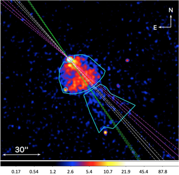
Figure 1. Merged exposure-corrected ACIS image (0.5–8.0 keV, smoothed with an r = 15 Gaussian kernel) with the following spectral extraction regions shown: pulsar/core (
 circle), compact nebula (CN) region (northern cyan polygon), and the mushroom “stem” region (southern cyan polygon). The magenta lines represent the direction of proper motion (
 east of north) as measured by Chatterjee et al. (2004), the white lines represent the direction of proper motion after the effects of solar motion and Galactic rotation have been removed (
 Hobbs et al. 2005), and the green lines represent the measured symmetry axis
  of the CN (see below). The point source that appears near the southeastern trailing edge of the CN (shown by the crossed circular region) was excluded from the CN spectral analysis. The color bar is in units of counts
Download figure:
Standard image High-resolution image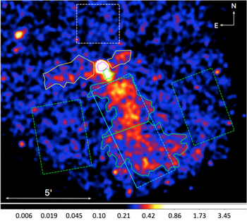
Figure 2. Merged 0.5–8 keV exposure-corrected image produced from all eight ACIS-I observations with point sources (detected by wavdetect) removed. The image is binned by a factor of eight ( pixel size), and smoothed with an
  Gaussian kernel. The following spectral extraction regions are shown: the tail (green contour region; the line separates the “near” and “far” halves), and the “whiskers” (yellow polygons on either side of the CN). The two green dashed rectangles to the sides of the tail are the background regions used in the tail’s spectral fits. The cyan
  rectangular region (along the tail contour) is used to extract the tail brightness profile (see Figure 5). The CN (magenta polygon) and stem (green polygon) are also shown (same regions as in Figure 2), along with the background region (dashed white box) used in the pulsar, CN, stem, and whiskers spectral fits. The level for the green contour was chosen in such a way that it conforms to the tail morphology at the contrast shown. The color bar is in units of counts arcsec
Download figure:
Standard image High-resolution image3.1.1. Pulsar Vicinity
We begin our analysis by studying the pulsar’s vicinity. This requires modeling and subtracting a point (unresolved) source at the location of the pulsar. We simulated point-source images (produced for each observation because of the differing roll angles and slightly different off-axis angles; see Table 2), combined them, and then subtracted them from the merged image of real data. However, the simulated PSF (the blue curve in Figure 3) under-predicts the width of the PSF for both B0355 and CXOU J035905.2+541455, a nearby point source used for comparison. Therefore, we do not consider the MARX simulation to be reliable for the purpose of our analysis here.
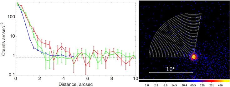
Figure 3. Comparison of the MARX simulated point-source radial profile (blue error bars), the nearby field point-source radial profile (CXOU J035905.2+541455; green error bars), and the observed count distribution (red error bars) in the area ahead of the moving pulsar (shown in the right panel). All profiles are normalized to the same value at the origin. The average background surface brightness (0.854 ± 0.014 counts arcsec−2) shown by the dashed horizontal gray line was added to the simulated point-source plot (blue). The simulated point source (blue curve) appears to under-predict the actual width of the PSF (compared the green curve), thus we do not consider the MARX simulations to be reliable for the purpose of our analyses. The color bar (right panel) is in units of counts arcsec .
.
Download figure:
Standard image High-resolution image3.1.2. Compact Nebula (CN)
The deep merged images produced from all eight ACIS-I observations (Figures 1 and 2) reveal the CN morphology, which can be described as a filled dome (or a mushroom cap when viewed together with the faint extension—the mushroom “stem”). The central region of the CN appears brighter than the sides. There is a clearly defined trailing edge beyond which the CN brightness falls off very abruptly. The sharp trailing edge is not straight and has a noticeable curvature to it.
To measure the direction of the symmetry axis of the PWN, we calculated the sum of CN counts on both sides of the green line (shown in Figure 1), which is rotated around the pulsar position until the number of counts is the same for each side. The 1σ uncertainties in the direction of the symmetry axis (dashed green lines) correspond to the 1σ deviation between the numbers of counts in the two parts of CN.
We compared the individual images of the CN to look for possible variability. The flux for the entire CN as a function of time is plotted in Figure 4. Fitting the resulting light curve with a constant,  erg cm−2 s−1, (the average of the individually fitted fluxes listed in Table 2) yields a reduced
  for
for  degrees of freedom (dof), consistent with the lack of significant variability. We also examined the structural changes in the subsequent CN images and could not identify any systematic variations in the CN structure.
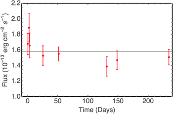
Figure 4. Unabsorbed fluxes (0.5–8 keV, see Table 2) of the individual fits of the CN region (shown in Figure 1). The gray line represents the average of the fluxes,  erg cm−2 s−1. These results are comparable to the CN flux from the archival ACIS-S observation (ObsID 4657),
  erg cm−2.
Download figure:
Standard image High-resolution image3.1.3. Mushroom Stem
A fainter emission protruding from the trailing edge of the CN in the direction opposite to that of the pulsar’s proper motion (the “stem” of the mushroom) is visible up to  . The stem is clearly resolved in the transverse direction, becoming wider (but fainter) with the increasing distance from the pulsar. The stem region is (on average) about a factor of six dimmer (in terms of surface brightness) than the CN. It may be composed of two structures that originate at the pulsar and slightly diverge from each other (with a half-angle of about 7°) further away, accounting for the apparent broadening of the stem with distance from the pulsar. If the stem indeed originates from the pulsar, it could account for the enhanced surface brightness along the symmetry axis of the CN. The stem is also seen in the first short Chandra observation; though, it is not as well resolved.
3.1.4. Tail
A diffuse tail is discernible up to at least  southwest of the pulsar (limited by the ACIS-I field of view), in the direction roughly opposite that of the pulsar’s proper motion. The tail’s average surface brightness (within the contour region shown in Figure 2) is dimmer than that of the CN by a factor of 40. The tail widens with distance from the pulsar and, for the part farthest from the pulsar, has a slightly lower average surface brightness (see Table 3). We show the tail’s surface brightness as a function of distance from the pulsar in Figure 5.
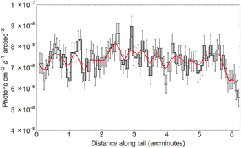
Figure 5. Tail brightness profile as a function of distance from the pulsar, for the rectangular tail region shown in Figure 2. The profile was obtained from the 0.5–8 keV exposure-map-corrected ACIS-I image binned by a factor of eight (corresponding to a pixel size of  ). The red curve represents the brightness profile when smoothed with a
  Gaussian kernel).
Download figure:
Standard image High-resolution imageTable 3. Spatially Resolved Spectra of PWN Regions
| Region | Area | I | Γ |

|

|
Reduced 
|

|
LX |

|
|---|---|---|---|---|---|---|---|---|---|
| (arcsec2) | (cts arcsec−2) | (dof) | (1031 erg s−1) | ||||||
| Pulsar/core | 9.44 | 80.8 ± 2.9 |

|
0.83 ± 0.09 | 88 | 1.37 (32) | −13.38 ± 0.02 | 0.54 | −3.92 |
| Pulsar/corea | 9.44 | 80.8 ± 2.9 |

|
0.51 ± 0.16 | 54 | 1.14 (30) | −13.21 ± 0.03 | 0.80 | −3.75 |
| CN | 791 | 3.45 ± 0.07 |

|
2.2 ± 0.10 | 2.8 | 0.96 (159) | −12.85 ± 0.01 | 1.83 | −3.39 |
| Whiskers | 14726 | 0.067 ± 0.008 |

|
0.48 ± 0.12 | 0.03 | 1.32 (33) | −13.44 ± 0.06 | 0.47 | −3.98 |
| Stem | 824 | 0.55 ± 0.03 |

|
0.36 ± 0.05 | 0.44 | 0.82 (59) | −13.70 ± 0.03 | 0.26 | −4.24 |
| Tail (Entire) | 59041 | 0.087 ± 0.004 |

|
5.4 ± 0.36 | 0.091 | 1.13 (135) | −12.53 ± 0.02 | 3.8 | −3.07 |
| Tail (Near) | 24223 | 0.11 ± 0.004 |

|
2.3 ± 0.21 | 0.095 | 1.38 (43) | −12.90 ± 0.02 | 1.6 | −3.44 |
| Tail (Far) | 34818 | 0.070 ± 0.004 |

|
3.1 ± 0.28 | 0.089 | 1.15 (69) | −12.79 ± 0.02 | 2.1 | −3.33 |
Note. Spectral fits for the extraction regions shown in Figures 2 and 3 with an absorbed PL model. The NH is fixed at  cm−2, which is the best-fit value for the CN and tail spectra (when fitted independently). The net surface brightness I (in cts arcsec−2) is listed for each region.
  is the average spectral surface brightness at E = 1 keV (photons s−1 cm−2 keV−1 arcsec−2), where
  is the normalization of the photon spectral flux from the PL fits (photons s−1 cm−2 keV−1) measured in area A. Unabsorbed flux FX, luminosity LX, and X-ray efficiency
  are for the distance of 1.04 kpc and correspond to the 0.5–8 keV range.
Download table as: ASCIITypeset image
3.1.5. Whiskers
Two very faint structures (“whiskers”) are discernable on either side of the CN, extending almost orthogonally to the direction of the tail and the pulsar’s proper motion. Despite their faint appearance, 433 net (background-subtracted) counts were detected from the combined whiskers region, yielding an S/N of 3.2. Compared to the CN, the whiskers are dimmer by a factor of about 50, making them slightly fainter than the tail in terms of the average surface brightness. The whiskers do not appear to be bent back by the ram pressure caused by the pulsar’s motion. The eastern whisker appears to be approximately twice the length of the western one ( versus
  , respectively).
3.2. Spatially Resolved Spectra
We extracted the spectra of the core/pulsar, CN, stem, whiskers, and the extended tail for the eight observations listed in Table 2 and fitted them. We also split the tail into two sub-regions: the near-half and far-half (as shown in Figure 2). All spectra were fitted satisfactorily with an absorbed power-law (PL) model, except for the pulsar/core region, which is best fit with a PL+blackbody (PL+BB) model. Fitting the CN spectrum yields the hydrogen column density  cm−2 (a comparable, albeit less certain value is obtained from the fit of the tail spectrum).20
We fix the
cm−2 (a comparable, albeit less certain value is obtained from the fit of the tail spectrum).20
We fix the  at this value, while fitting the spectra of other regions (see Table 3) because of the poorer statistics. For each of the regions, we simultaneously fit the data from all eight observations used (see Table 3). The photon indices for the pulsar/core and the CN are
  and
and  , respectively. The indices are virtually the same for both halves of the tail:
  for the near-half of the tail, and
  for the far-half, while
  for the entire tail. For the whiskers,
  with
with  for
for  d.o.f., and for the stem,
  with
with  for
for  d.o.f. For illustration, the merged tail spectrum is shown in Figure 6.
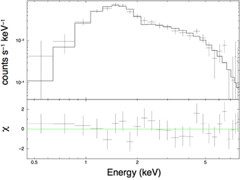
Figure 6. ACIS-I spectrum for the entire tail obtained by merging the spectra from eight observations. The best fit shown corresponds to an absorbed PL with  and
and  . The merged spectrum is shown for illustrative purposes only. See Table 3 for details.
Download figure:
Standard image High-resolution imageOur spectral measurements are more accurate than those obtained from the earlier Chandra and XMM-Newton observations. As a result, we can better constrain possible spectral changes due to synchrotron cooling. We observe only a hint of softening,  , between the CN and pulsar tail, while virtually no spectral slope change is seen between the two halves of the tail. We discuss the implications of these findings in Section 4.
The softer spectrum and rather poor quality of the pulsar/core region PL fit ( ) suggests a possible contribution of thermal emission from the neutron star (NS) surface, which can be approximated by a blackbody (BB) model. A PL+BB model provides a better quality fit (
 ), yielding
  ,
,  keV, and the projected emitting area
  km2, where the first and second number in parentheses correspond to the
  lower and upper bounds of the parameter. The improvement in the fit quality due to the addition of the BB component is significant at the 97.6% level according to the F-test. Figure 7 shows the contribution of the thermal component at lower energies (left panel) and constraints on the temperature and size of the emitting region (right panel).
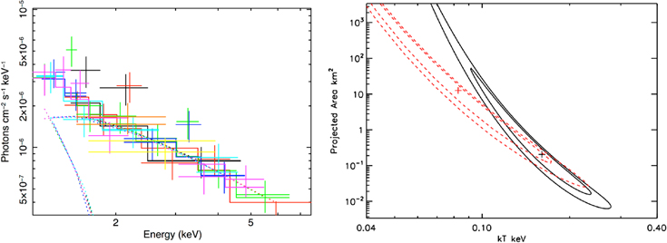
Figure 7. Left: plot of the unfolded spectrum fitted with a PL+BB model. Right: contour plot of the projected emitting BB area vs. temperature for the PL+BB fit (black solid line) and a similar plot for the PL+NSA fit to the pulsar/core region (red dashed line; 1σ and 2σ confidence contours are shown for both plots).
Download figure:
Standard image High-resolution image4. DISCUSSION
As described above, the PWN morphology is quite complex, with feature scales varying from arcseconds to arcminutes. Overall, the X-ray images are dominated by the PWN (i.e., all regions except the pulsar/core), whose luminosity in 0.5–8 keV,  erg s−1, exceeds that of the unresolved pulsar/core by a factor of 13. Below, we discuss and attempt to interpret the individual features of the PWN.
4.1. Core/Pulsar
The superior quality of the PL+BB fit (compared to the PL fit) suggests the presence of a soft thermal component in addition to the PL, whose slope is comparable with the CN slope. The large uncertainties of the thermal component and, particularly, the poorly constrained size of the emitting area (see Figure 7) do not allow us to make a firm conclusion on whether the thermal component comes from the bulk of the NS surface or from a hot polar cap. If the emission comes from the surface of an  km NS surface, the fit implies
  MK, which is hotter than what is expected from standard cooling at B0355's spin-down age (Yakovlev & Pethick 2004) and falls outside the
  contour shown in Figure 7. The temperature would be lower, ∼0.6 MK, if the NS (with the same radius) has a hydrogen atmosphere (NSA model; Pavlov et al. 1995). Alternatively, the thermal component could be attributed to a hot (
 MK) spot with the size (
 m), comparable to the size of a pulsar’s polar cap,
  m.
m.
Although the emission from the pulsar/core appears to be centrally peaked, we cannot claim with absolute confidence that it represents the pulsar emission until pulsations are detected.21 It is unlikely that the termination shock (TS) is hidden inside the unresolved core because this would imply an improbably large pulsar velocity (see estimates below).
4.2. Compact Nebula (CN)
4.2.1. Bow Shock and Pulsar Velocity
The cometary shape of the CN indicates that the pulsar wind flow is deflected by the ram pressure of the ISM. Comparing the brightness profile of the region ahead of the pulsar with the radial profile of the field point source CXOU J035905.2+541455, we find that the emission at the CN apex becomes distinguishable from the background at a distance of  in front of the pulsar (see Figure 3), which corresponds to the projected stand-off distance
  cm. Balancing the ram pressure of the ISM with the isotropic pulsar wind pressure22
,
cm. Balancing the ram pressure of the ISM with the isotropic pulsar wind pressure22
,  , where
  is the mass of the hydrogen atom,
  is used to convert H density to total density of the ambient medium, and
  is the pulsar velocity, allows us to estimate the ISM number density
  cm−3 (where i is the angle between the pulsar velocity and the line of sight). The exact inclination angle i is not known; however, it cannot be too different from 90◦ given that the stand-off distance
  is small compared to the size of the CN. Based on the pulsar’s Galactic coordinates (
 ,
,  ) and the
  distance, it is reasonable to assume that the ISM is in the “warm” phase (see Cox 2000), with sound speeds of
  km s−1 and the Mach number,
  , is (5–8)/
 , depending on the value of cs and the inclination angle i.
For highly supersonic motion and small values of the magnetization parameter of the initially isotropic pre-shock pulsar wind, the TS bullet’s cylindrical radius  , while the lengths of the TS bullet is expected to be
  (Gaensler et al. 2004; Bucciantini et al. 2005, hereafter B+05). This provides a poor match to the observed shape of the CN, which can be described as a dome rather than a bullet. In addition to the expected anisotropy of the pulsar wind, it is likely that the motion of the pulsar in this case is only mildly supersonic; however, low-
 simulations (van der Swaluw et al. 2003) fail to reproduce the dome-shaped TS as well. It is reasonable to expect that the CN could become wider (compared to isotropic wind scenario) if the outflow is dominated by the equatorial component perpendicular to the pulsar velocity vector. In this case, the toroidal structure associated with the TS23
will be deformed and pushed back by the ram pressure of the oncoming medium. Evidence for such a transitional deformation between the toroidal structure and cometary shapes is seen in the Vela PWN (see Figure 2 in Pavlov et al. 2003), the IC443 PWN (Swartz et al. 2015) and, perhaps, in the CTB 80 PWN (moon et al. 2004).
simulations (van der Swaluw et al. 2003) fail to reproduce the dome-shaped TS as well. It is reasonable to expect that the CN could become wider (compared to isotropic wind scenario) if the outflow is dominated by the equatorial component perpendicular to the pulsar velocity vector. In this case, the toroidal structure associated with the TS23
will be deformed and pushed back by the ram pressure of the oncoming medium. Evidence for such a transitional deformation between the toroidal structure and cometary shapes is seen in the Vela PWN (see Figure 2 in Pavlov et al. 2003), the IC443 PWN (Swartz et al. 2015) and, perhaps, in the CTB 80 PWN (moon et al. 2004).
Since the CN is highly symmetric, we measured the orientation of the axis of symmetry (projected onto the sky plane) as  east of north (which coincides with the approximate axis of symmetry of the tail; see Section 3.1.2). This angle is noticeably different (
 ) from the velocity vector’s angle of
  east of north as reported by Hobbs et al. (2005), who removed effects of solar motion and Galactic rotation from the values obtained by Chatterjee et al. (2004) based on VLBA observations (see Figure 1). The mismatch could be explained by the motion of the ISM, since the axis of symmetry should trace the relative speed of the pulsar with respect to the ISM, and not its absolute direction. If the mismatch is indeed attributed to ISM motion, it would imply a projected bulk ISM flow velocity
  (directed southeast, perpendicular to the pulsar’s direction of proper motion (the white line in Figure 1).
4.2.2. CN Morphology
The CN of B0355 features a “filled” morphology with the central region of the CN being noticeably brighter than the sides (see Figure 1). Such an appearance is in stark contrast with the “hollow” morphologies of the Geminga and PSR J1509–5850 PWNe (Pavlov et al. 2010 and Klingler et al. 2016), but similar to that of the (filled) Mouse PWN (Gaensler et al. 2004). If the spin axis of B0355 is directed close to the line of sight, the brighter central region of the CN could represent the jets (launched along the NS spin axis) that are being swept back by the ram pressure of the oncoming ISM. In this interpretation, the jets appear to be superimposed on the sky close to each other, but they separate slightly beyond the trailing edge of the CN, contributing to the split appearance of the stem (see Figures 1 and 2). Note that this scenario explains the nearly symmetric disposition of the split stem about the axis of symmetry. If axisymmetric sweepback provides the only perturbation of twin polar jets, then we can use the stem opening half-angle to infer that the angle between the proper motion and the projected jet axis is  . For such a small angle, the jets would appear nearly straight, as observed, but unless the jet axis is projected very close to the proper motion axis, the full angle to the line of sight is small:
  (1 σ) and
  (90% confidence level).
In fact, there is a good reason to believe that the spin axis of B0355 is nearly aligned with our line of sight, since it is not detected in the γ-ray band. Indeed, Romani et al. (2011) showed that B0355 is one of the “subluminous” γ-ray pulsars (objects fainter than expected from their spin-down parameters), and argued from radio emission properties that this is an orientation effect. As shown by Figure 3 of Romani et al. (2011), the radio pulse properties imply a spin axis within  of the line of sight, where indeed γ-ray pulses would not be visible. Geminga and PSR J1509–5850, in contrast, are γ-loud and hence must be viewed nearly orthogonally to the spin axis. We thus expect that their swept-back jets would lie near the plane of the sky and are widely separated and highly curved24
, as observed (Klingler et al. 2016; Posselt et al. 2016).
of the line of sight, where indeed γ-ray pulses would not be visible. Geminga and PSR J1509–5850, in contrast, are γ-loud and hence must be viewed nearly orthogonally to the spin axis. We thus expect that their swept-back jets would lie near the plane of the sky and are widely separated and highly curved24
, as observed (Klingler et al. 2016; Posselt et al. 2016).
Note that, while there is a statistical trend for spin and proper motion vectors to be aligned (e.g., Ng & Romani 2007), there are examples of highly misaligned objects (e.g., the IC433 PWN and PSR B1706−44, Swartz et al. 2015 and Romani et al. 2005, respectively). One conclusion of Ng & Romani (2007) is that, for the kick models studied, misalignment should be most common for pulsars with low space velocities. B0355's low velocity supports this hypothesis.
Orientation alone can hardly explain the contrasting morphologies of CNe observed in several of the PWNe mentioned above. For example, the Mouse PWN (Gaensler et al. 2004) and PSR J1741–2054's PWN (Auchettl et al. 2015) do not show any strong jet component, and may be dominated by equatorial outflows. Two pulsars with jets likely aligned with our line of sight, PSRs B0656+14 and B1055–52 (Bîrzan et al. 2016; Posselt et al. 2015, respectively), have very faint PWNe. Other factors, such as the spin-magnetic axis angle, and the angle between the spin axis and velocity vector, must control the relative brightness of the polar and equatorial wind components.
4.3. Stem and Tail
The visible (projected) length of the pulsar tail spans  (2.1 pc at d = 1.04 kpc) behind the pulsar. It is possible that the actual length is larger, but it would then be outside the ACIS-I field of view. Beyond
  from the pulsar, the tail broadens and drops noticeably in surface brightness (see Figure 2). The near-half of the tail (the one that is closer to the pulsar) appears to be more or less symmetric with respect to the CN symmetry axis, while the second half seems to bend ∼30° south, and expand. Although the symmetry axis of the PWN and tail may not exactly align with the proper motion direction in the case of anisotropic pulsar wind (Vigelius et al. 2007), such distortions caused by misalignment are not expected to manifest themselves at large distances from the pulsar. Thus, the observed bending could be caused by ISM pressure nonuniformity, instabilities in the tail flow, or ISM entrainment, which brings the flow close to being at rest with respect to the ambient medium. A similar bending is seen in the tail of PSR J1741–2054; however, its morphology is somewhat different because it appears to be composed of expanding bubble structures (Auchettl et al. 2015). Despite the sharp drop in the surface brightness behind the trailing edge of the CN, there appears to be only modest (if any) spectral changes between the CN, the stem, and the tail. The spectrum softens by
  between the CN and the tail (see Table 3 and Figure 8), suggesting that the sharp drop in brightness25
(a factor of
between the CN and the tail (see Table 3 and Figure 8), suggesting that the sharp drop in brightness25
(a factor of  over a 5″distance) is not associated with rapid cooling but should rather be attributed to the rapid flow expansion or/and drop in magnetic field strength. Rapid expansion is expected in models that take into account ISM entrainment into the wind behind supersonically moving pulsars (see Figure 7 in Morlino et al. 2015).
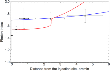
Figure 8. Photon index as a function of distance from the pulsar. Measured values are plotted as vertical black error bars ( ) where the leftmost one represents the core (pulsar), and the subsequent ones are the CN, stem, near-half, and far-half of the tail, respectively. The horizontal bars indicate the distance over which the photon index was measured. The red curve represents Equation (2) with the injection spectrum slope corresponding to that of CN (p = 2.08) and “best-fit”
  . The blue curve represents Equation (2) with the injection spectrum slope corresponding to that of the stem (p = 2.46) and
  . The break in the red curve occurs at the distance, where
  .
.
Download figure:
Standard image High-resolution imageA similarly small spectral evolution is seen between the compact PWN and tail of PSR J1509–5850 (Klingler et al. 2016). On the other hand, much more pronounced spectral softening trends have been measured in the N157B ( , Chen et al. 2006), the Lighthouse (
 , Pavan et al. 2016), and the Mouse (Gaensler et al. 2004
  , N. Klingler et al. 2016, in preparation) PWNe.
4.3.1. Physical Properties
The magnetic field strength can be estimated from measurements of synchrotron surface brightness (see, e.g., Pavlov et al. 2003). For a given magnetization,  , where
  is the magnetic energy density and we is the energy density of relativistic particles, the magnetic field strength can be expressed as

In this equation,  is the average spectral surface brightness at E = 1 keV (photons s−1 cm−2 keV−1 arcsec−2),
  is the normalization of the photon spectral flux (from the PL fits) measured in area A,
  cm is the average length of the radiating region along the line of sight,
  ,
,  , Em and EM are the lower and upper energies of the photon PL spectrum (in keV), and
  ,
,  and ap are the numerical coefficients26
whose values depend on the slope,
and ap are the numerical coefficients26
whose values depend on the slope,  , of the electron spectral energy distribution (SED).
Table 3 lists Γ and  for the two sections of the tail and the CN, and
  can be assumed to be equal to the tail’s width. The magnetic field strength also depends on the boundary energies of the electron SED, which are poorly constrained because the tail is not detected outside the ACIS band. For the measured Γ and corresponding SED slopes, B is insensitive to the upper energy, EM, while the dependence on the lower energy, Em, is more appreciable. For instance, the magnetic field for the near-half would change from
  μG to
μG to  μG if
μG if  is replaced with
  keV (which corresponds to
  Hz). For the far-half, the B values are very similar,
  μG and
  μG, for the same Em values, respectively. For equipartition, the magnetic field estimates imply the tail energy densities
  erg cm−3, depending on the choice of Em. Using the same method, we estimate the CN magnetic field to be
  μG (depending on the value of Em). The Lorentz factor of electrons producing synchrotron photons with energy E can be estimated as
 . For particles carried by the flow in the pulsar tail, the time they will radiate in X-rays is limited by the synchrotron lifetime,

 years. Because no significant spectral cooling is seen in the B0355 tail,
  must be larger than the travel time
  , where u is the bulk flow speed (assumed to be constant here for simplicity) and
  pc is the length of the tail visible in X-rays. This requirement implies that the average flow speed
  km s−1, which significantly exceeds the pulsar velocity. Of course, the initial flow velocity in the tail is likely to be much higher than the estimated average value (see simulations by B+05), and the flow should eventually slow down to be at rest with the ISM at large distances.
One can also use a simple 1D model of a collimated outflow cooling solely via synchrotron radiation (e.g., Chen et al. 2006) to estimate the flow speed. In a cylindrical tail, where particles flow away from the pulsar with a constant velocity u in a constant magnetic field B, the photon index at distance z from the pulsar can be expressed as
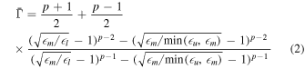
where  is the PL slope of the electron SED, which is assumed to produce a PL spectrum with the minimum and maximum energies,
  and
and  , and
, and

is the photon energy corresponding to particles of maximum energy Em at distance z, with account for synchrotron losses.
As one might expect, it is difficult to obtain a good correspondence between this simplistic model and the data, especially if the CN is included (red line in Figure 8). The model assumes a constant tail cross section, magnetic field, and velocity, while all of these parameters are likely to change substantially between the CN and the extended tail, and also within the tail. A seemingly satisfactory correspondence between the model and the data can be obtained if the injection is assumed to be happening further downstream (i.e., outside of CN) where the injection spectrum has a larger p (corresponding to the somewhat softer Γ than we measured). One can obtain reasonable fit as long as  , corresponding to
  km s−1, which is comparable to the simpler (monoenergetic) estimate given above.
For a cylindrical flow of radius  , the corresponding average energy injection rate into the tail can be estimated as
 . Assuming equipartition (wB = we) in the B0355 tail,

 , implying that
  of the pulsar’s spin-down power (
 ) is transferred to the plasma flowing down the tail.
An alternative (to the high flow velocity) explanation of the slow cooling in the tail could be reacceleration of the particles powered by turbulence in the tail plasma with the energy being taken from the magnetic field (e.g., via reconnection). However, the available X-ray data do not provide a way to discriminate between the two possibilities. The second scenario could be more favored in cases when the radio surface brightness of the tail increases with the distance from the pulsar (e.g., the tail of PSR J1509–5850; Ng et al. 2010; Klingler et al. 2016). So far, no radio emission has been detected from the B0355 tail. Thus, sensitive lower frequency observations (e.g., IR and radio) are needed to determine a more accurate low energy break for the particle spectrum and a more accurate lower limit on the inferred magnetic field.
The above estimates neglect possible diffusion of the synchrotron emitting particles. Particle transport models with synchrotron radiation losses are widely used to simulate the spatial and spectral properties of PWNe, such as the Crab Nebula, 3C 58, G21.5–0.9, and others (see, e.g., Wilson 1972, and Tang & Chevalier 2012; Porth et al. 2016). The diffusion coefficient is typically a free parameter in such models. The maximal spatial extension of the synchrotron tail in the one-dimensional diffusion model (assuming the lack of strong evolution of the magnetic field)  . This allows us to constrain the diffusion coefficient D of the synchrotron emitting electrons to be
  cm2 s−1. Both Wilson (1972) and Tang & Chevalier (2012) discussed simplified diffusion models in which D is assumed to be energy-independent for synchrotron emitting electrons. The constraints obtained above for the X-ray nebula created by PSR B0355+54 is consistent with the typical numbers used by Tang & Chevalier (2012 see their Figure 9, where a much higher magnetic field was assumed to fit the radio through optical data of the Crab Nebula). Models of the plasma turbulence in relativistic outflows (Bykov & Treumann 2011) typically predicted energy-dependent diffusion coefficients, which are increasing with the particle energy. The constraint given above is actually close to the so-called Bohm diffusion coefficient,
  , where Rg is the particle gyroradius. The value DB usually corresponds to the minimal possible value of the diffusion coefficient in the magnetic turbulence. The above estimates may be even more appropriate for the whiskers (see Section 4.4), where they would lead to similar conclusions.
4.4. Whiskers
Outflows strongly misaligned with the pulsar velocity have been seen in three other PWNe created by supersonic pulsars: the Guitar Nebula (PSR B2224+65; Hui & Becker 2007), the Lighthouse PWN (IGR J11014–6103; Pavan et al. 2014, 2016) and the PWN of PSR J1509–5058 (Klingler et al. 2016). Bandiera (2008) suggested that such structures can occur when the stand-off distance at the apex of the bow shock,  , becomes smaller than the electron gyration radius,
  . If true,27
this would imply that
. If true,27
this would imply that  (here
(here  is the PWN magnetic field near the bow shock apex). In such a scenario, high-energy particles can “leak” into the ISM, where they diffuse along the ambient magnetic field. Therefore, if the diffusion is fast, the orientation of the outflow reflects the geometry of the ambient magnetic field. As the whiskers do not appear to be bent back by the ram pressure, they are likely ambient ISM structures illuminated by pulsar-produced particles.
This scenario received support in the recent study of the Lighthouse PWN (Pavan et al. 2016), where evidence of draping of the ISM magnetic field lines around the bow shock head (Lyutikov 2006; Dursi & Pfrommer 2008) is seen in the Chandra ACIS image. If the  requirement is indeed a necessary condition for the leakage, it provides an additional link between pulsar and PWN properties, and decouples the ultra-relativistic electron energies from the often poorly constrained PWN magnetic field. Indeed, the Lorentz factor of electrons escaping into the ISM is
  (here
(here  is the ISM magnetic field), and hence one can constrain the magnetic field in the PWN head to be
  μG. This would imply that the magnetic field in the tail is likely close to the lower end of the range estimated in Section 4.3.1, and the magnetization should not be, in the Bandiera (2008) scenario, too far from the equipartition.
Consequently, the spectra of the misaligned outflows are expected to be relatively hard, as is observed in the Guitar ( ), the Lighthouse (
 ), and the J1509–5850 (
 ) spectra. In the case of B0355, the slope of the fitted PL is rather uncertain (
 ) but the best-fit value for the whiskers spectra is smaller than that for any other region except the CN. In the other three known instances, the outflows display a puzzlingly strong asymmetry, being much more prominent on one side of the pulsar than on the other. The outflows seen in the Guitar, J1509–5850, and the Lighthouse PWNe also appear to be better collimated, which could be the result of stronger, more ordered ambient magnetic fields. The relative surface brightness of the B0355 whiskers (dimmer than the CN by a factor of ∼70) is comparable to the relative surface brightness of J1509–5058's misaligned outflow (which is dimmer than the J1509–5058 CN by a factor of ∼50). More accurate spectral measurements for the extended tails and misaligned outflows should be possible with the Athena X-ray Observatory (Kargaltsev et al. 2015).
5. SUMMARY
We have presented a detailed analysis of the PWN created by the supersonic pulsar B0355+54. The deep Chandra observations show the presence of a bright CN and a  -long (∼2 pc) tail directed opposite the pulsar’s direction of proper motion.
The CN displays a filled dome morphology, with the center being the brightest (in contrast to the Geminga and J1509–5850 CNe), a sharp trailing edge, and two faint protrusions (the split “stem” region) extending beyond this edge. We hypothesize that this is the result of our line of sight being directed along (or close to) the pulsar spin axis, with the jets then being bent back by the ISM ram pressure caused by the proper motion, superimposed on the CN, causing the center to appear brighter. With such an interpretation, in “hollow” CNe morphologies (e.g., J1509–5850, Geminga), the brightened lateral regions could represent jets that are initially oriented at a larger angle with respect to the line of sight.
The emission from the pulsar and its immediate vicinity is softer, perhaps due to the presence of a thermal component, which could be attributed to emission from either the entire NS surface, implying  –0.8 MK, or from a ∼250 m hot spot with
  MK (for a BB model).
The tail shows no significant spectral softening up to 2 pc from the pulsar, suggesting a high bulk flow speed ( a few thousand km s−1) or in situ particle reacceleration is occurring within the tail.
The deep observations also suggest the presence of two faint structures extending from the bow shock CN, roughly perpendicular to the pulsar’s direction of motion. Similar outflows have been seen in other nebulae created by supersonic pulsars (the Guitar and Lighthouse PWNe), and are hypothesized to be the result of high-energy electrons diffusing out of the bow shock region and interacting with the ambient ISM magnetic fields.
We would like to thank Martin Weisskopf, Maxim Lyutikov, Giovanni Morlino, and Marina Romanova for the very helpful discussions. We are also grateful to the anonymous referee for the helpful suggestions and a careful reading of the paper. Support for this work was provided by the National Aeronautics and Space Administration through Chandra Award Number G03-14082 issued by the Chandra X-ray Observatory Center, which is operated by the Smithsonian Astrophysical Observatory for and on behalf of the National Aeronautics Space Administration under contract NAS8-03060. The work was also partly supported by NASA grant NNX08AD71G. A.M.B. was supported by RSF grant 16-12-10225.
Facility: CXO. - Chandra X-ray Observatory satellite
Footnotes
- 15
- 16
- 17
- 18
- 19
- 20
Alternatively, fitting together the pulsar, CN, and tail regions simultaneously with a tied
 and free Γ values and normalizations gives cm−2, which is within 1.6σ of the value for the CN (see Table 3). The results from this approach do not significantly differ from those listed in Table 3. Therefore, we use the value obtained from the CN fit, as it had the best constrained Γ.
 - 21
A search for pulsations in our data is not possible because the ACIS-I data was taken in Full Frame mode, which has a coarse 3.2 s timing resolution. The timing analysis of the XMM-Newton data by McGowan et al. (2006) produced only marginal detection of a pulsed signal, likely because of substantial contamination by CN photons.
- 22
Note that isotropic pulsar wind is assumed for simplicity.
- 23
Note that the sizes of the toroidal structures seen in a number of PWNe (KP08) can be substantially larger than the TS shock size, e.g., in the Crab PWN, the torus is a factor of three larger than the size of the inner ring (Weisskopf et al. 2000).
- 24
This is assuming that the spin and velocity vectors are substantially misaligned.
- 25
In the Vela PWN, the brightness change between the arcs (presumably associated with the termination shock) is only a factor of 1.5–2 over 3″–4″ length scale comparable to 1″ at the B0355's distance.
- 26
See Table 2 in Ginzburg & Syrovatskii (1965).
- 27
This requirement may be violated if there is an ongoing reconnection between the internal PWN and external ISM magnetic fields, in which case particles with smaller γ could leak as well (M. Lyutikov 2016, private communication).




