Abstract
We present numerical simulations of misaligned disks around a spinning black hole covering a range of parameters. Previous simulations have shown that disks that are strongly warped by a forced precession—in this case, the Lense–Thirring effect from the spinning black hole—can break apart into discrete disks or rings that can behave quasi-independently for short timescales. With the simulations we present here, we confirm that thin and highly inclined disks are more susceptible to disk tearing than thicker disks or those with lower inclination, and we show that lower values of the disk viscosity parameter lead to instability at lower warp amplitudes. This is consistent with detailed stability analysis of the warped disk equations. We find that the growth rates of the instability seen in the numerical simulations are similar across a broad range of parameters, and are of the same order as the predicted growth rates. However, we did not find the expected trend of growth rates with viscosity parameter. This may indicate that the growth rates are affected by numerical resolution, or that the wavelength of the fastest-growing mode is a function of local disk parameters. Finally, we also find that disk tearing can occur for disks with a viscosity parameter that is higher than predicted by a local stability analysis of the warped disk equations. In this case, the instability manifests differently, producing large changes in the disk tilt locally in the disk, rather than the large changes in disk twist that typically occur in lower-viscosity disks.
1. Introduction
Accretion disks are generally considered to orbit their central accretor in a smooth sequence of planar and circular orbits. However, there is a substantial body of observational evidence that shows that real disks are more complicated. For example, warped disks are used to model the X-ray binary Her X-1 (e.g., Scott et al. 2000), water masers reveal disks warps around supermassive black holes (e.g., Miyoshi et al. 1995; Greenhill et al. 1995), and the recent spatially resolved observations of protoplanetary disks have directly revealed complex disk structures including disk warps (e.g., Casassus et al. 2015). Very recently, it has been suggested that a misalignment between the gas and black hole angular momentum may be required to resolve discrepancies in the mass measurements for the supermassive black hole in M87 that was imaged by the Event Horizon Telescope (Jeter & Broderick 2021). Warps may form in different ways in different systems. For example, warps can form during the formation of an accretion disk, e.g., in chaotic star-forming regions (Bate et al. 2010; Bate 2018), or the disk may become warped if the orbits are forced to precess in a radially differential manner by the spin of the central object, e.g., a spinning black hole (Bardeen & Petterson 1975) or the gravitational field of a binary system (Papaloizou & Terquem 1995; Larwood & Papaloizou 1997).
To a first approximation, warps can propagate through a disk in one of two ways dependent on the relative magnitudes of the Shakura & Sunyaev (1973) dimensionless viscosity parameter, α, and the disk angular semi-thickness, H/R (Papaloizou & Pringle 1983). For low-viscosity disks, where α < H/R, warps propagate via bending waves. For high-viscosity disks, where α > H/R, warps propagate following a diffusion equation. In this work, we are principally interested in the diffusive case, although we do present some simulations with α ≲ H/R. For a review of the basics of warped disk dynamics, see Nixon & King (2016).
Recently, it has become possible to explore detailed dynamics of warped disks with numerical hydrodynamical simulations. There is now a broad range of simulations covering a variety of astrophysical setups, including; (1) isolated warped disks (e.g., Nelson & Papaloizou 1999; Lodato & Price 2010), (2) warped disks in binary systems (e.g., Larwood et al. 1996; Larwood & Papaloizou 1997; Fragner & Nelson 2010), and (3) warped disks around spinning black holes (e.g., Nelson & Papaloizou 2000; Fragile et al. 2007). A recurring feature of the warped disks in simulations is that they can “break” or “tear” (e.g., Nixon et al. 2012a), and this typically occurs when the simulation parameters allow for large enough warp amplitudes (either present at the start of the simulation, or formed over time) at sufficiently low viscosity.
The warp amplitude, ψ, is given by 3

where R is the orbital radius, and
l
(R, t) is the unit “tilt” vector pointing in the direction of the disk angular momentum vector. The unit tilt vector is usually written as  , where β(R, t) is the disk “tilt” and γ(R, t) is the disk “twist”. From this, we can see that disks can be warped in distinct ways. For example, a disk may achieve a warp (ψ > 0) if β varies with radius or if γ varies with radius (and β ≠ 0). We illustrate these two cases in Figure 1. As we shall see below, a large warp amplitude can be caused by a sharp variation in β or a sharp variation in γ. In general, a warped disk has both β and γ varying with radius. Locally, on scales ∼ H, the disk does not know whether misaligned neighboring rings are tilted or twisted with respect to each other, and thus the stability of the disk (as determined by a local stability analysis) is determined by ψ and not β or γ. However, as we shall see below the global behavior of the disk can result in the local instability manifesting as either a sharp change in the disk twist (Nixon et al. 2012a) or a sharp change in the disk tilt (see Section 3.5).
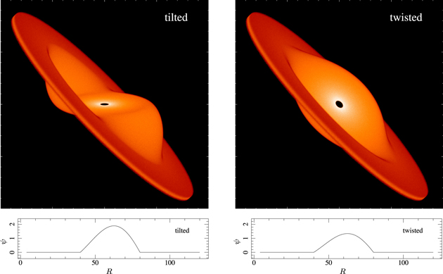
Figure 1. Example disk structures depicting the way in which a disk can be warped. On the left-hand side, we show a three-dimensional rendering of a warp imposed on a disk where only the tilt angle, β, varies with radius. On the right-hand side, we show a similar structure, but this time only the disk twist angle, γ, is varied with radius. In each case, the inner disk radius is at R = 4, and the outer disk radius at R = 120. For the tilted case, we take γ = 0° at all radii, while β = 0° for R < 40 and β = 45° for R > 80. Between these two radii, we vary β smoothly from 0° to 45° with a cosine bell. This results in the warp amplitude with radius, ψ(R), shown in the plot below the image; in this case, we have  . For the twisted case, we take β = 45° at all radii, with γ = 0° for R < 40 and γ = 45° for R > 80. Between these two radii, we vary γ smoothly from 0° to 45° with a cosine bell. This results in the warp amplitude with radius, ψ(R), shown in the plot below this image, and in this case we have
 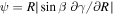 . We have shown these disks in an orientation in which the outer plane is the same in each case.
Download figure:
Standard image High-resolution imageThe nomenclature for unstable warped disks, i.e., “break” and “tear,” is ill-defined in the literature. By a disk “break,” we mean (see also, e.g., Doğan et al. 2018) that the disk has a sharp transition in either the disk tilt angle (β) or the disk twist angle (γ), and that this is usually accompanied by a sharp variation in the disk “surface” density 4 at the same radius. Breaks may arise in a warped disk that achieves a sufficient warp amplitude, and can occur with or without a forced precession of the disk orbits (see, e.g., Nixon & King 2012). The necessary conditions for disk “breaking” are discussed by Doğan et al. (2018) and Doğan & Nixon (2020). By disk “tearing,” we mean that an otherwise stable disk has been forced to precess (differentially) sufficiently rapidly that it achieves a large enough warp amplitude that renders the disk unstable to disk “breaking,” and that the resulting parts of the broken disk are able to subsequently precess quasi-independently before interacting in a highly dynamic and variable fashion. With this nomenclature, we define disk “breaking” as the underlying instability (see Doğan et al. 2018), and disk “tearing” refers to the action of breaking a disk with a forced precession and the subsequent dynamical behavior of the unstable disk (see Nixon et al. 2012a).
Larwood et al. (1996) and Larwood & Papaloizou (1997) present numerical simulations using smoothed particle hydrodynamics (SPH) of misaligned disks in binary systems, including both the circumbinary disk case and the case where the companion is external to the disk. In each case, they show a simulation, typically the thinnest simulation presented, that exhibits disk tearing; the gravitational torque on the disk causes the disk orbits to precess and a break is formed between the inner and outer regions of the disk. They note that, in these models, the sound speed is too low to allow efficient communication between the different regions of the disk. Similar results are presented by Fragner & Nelson (2010), who modeled the hydrodynamics using a grid code. These investigations exhibit disk tearing (breaking of the disk caused by a forced precession), but did not follow the evolution for long enough to explore the subsequent nonlinear, chaotic behavior. The dynamical behavior of disk tearing was explored by a series of papers in different contexts: disks around spinning black holes (Nixon et al. 2012a), circumbinary disks (Nixon et al. 2013), and disks with an external binary companion (Doğan et al. 2015). These simulations reveal the quasi-independent precession of rings of matter (some of which are radially narrow with ΔR ∼ H, and others more extended with ΔR ≫ H). These rings are found to precess until the internal angle between two neighboring rings becomes large, at which point they can interact violently, with shocks between rings producing gas on low angular momentum orbits that can fall to smaller radii. This material can fall directly on to the central accretor or circularize at a new, smaller radius. These processes can dramatically change the disk evolution and its observational character; for further discussion, see, e.g., Nixon & Salvesen (2014). Over the last few years, disk tearing has been explored in the low-viscosity case (Nealon et al. 2015), has been found in general relativistic magnetohydrodynamic simulations (Liska et al. 2021), and has been used to model observations of the circumstellar disk in GW Ori (Kraus et al. 2020).
Recently, Doğan et al. (2018) connected the disk breaking and tearing behavior observed in numerical simulations with the instability of warped disks that was derived by Ogilvie (2000) through a local stability analysis of the warped disk equations. Ogilvie (1999) showed that, in some circumstances, as the warp amplitude is increased, the local “viscosity” that resists the warping, e.g., ν2 (Pringle 1992) decreases. Thus, the more warped the disk gets, the less it is able to resist warping further. This is found to occur for viscosities that are not much larger than α = 0.1, and at a critical warp amplitude, ψc, that depends on α; typically, lower α yields lower critical warp amplitudes. While Doğan et al. (2018) focused on disks with Keplerian rotation, Doğan & Nixon (2020) explored the instability in the case of non-Keplerian rotation.
Here, we perform numerical hydrodynamical simulations to explore the instability of warped disks and the disk-tearing behavior. To provide the forced precession, we simulate disks around spinning black holes, and we vary the disk parameters, including the viscosity parameter α, the disk angular semi-thickness H/R, and the inclination of the disk θ, with respect to the rotation axis of the black hole. In Section 2, we discuss the numerical methodology and expectations for the simulations. In Section 3, we report the results of the numerical simulations. In Section 4, we present our conclusions.
2. Numerical Considerations
In this section, we discuss the methodology that is employed in our numerical simulations (reported in Section 3 below), and how numerical effects may impact the results of our simulations. We use smoothed particle hydrodynamics (SPH) to model the accretion disk (see, e.g., Price 2012), and in particular, we use the SPH code phantom (Price et al. 2018). To generate a time-dependent warp in the disk, with which we can analyze the evolution, we perform simulations of disks that are misaligned to a central spinning black hole. This includes both apsidal (Einstein) precession of eccentric disk orbits, and nodal (Lense–Thirring) precession of misaligned disk orbits.
Following Nelson & Papaloizou (2000), we employ a post-Newtonian approximation to model the gravity of the black hole. We use the Einstein potential for the apsidal precession with a gravitomagnetic force term to induce the required Lense–Thirring precession; for details, see Nixon et al. (2012a) and Price et al. (2018).
5
While the Einstein potential provides a good description of the expected apsidal precession of the disk orbits, it does not produce an innermost stable circular orbit (ISCO) to define the inner edge of the disk. Instead, we place an accretion radius at the location of the ISCO in order to truncate the disk there. The ISCO is defined by the location where circular orbits become unstable, which is equivalent to the square of the dimensionless epicyclic frequency,  , becoming negative. In terms of the orbital shear parameter,
  , this is where q = 2. For the post-Newtonian approximation we employ, q increases as the radius decreases, but q < 2 by the time the ISCO is reached. For the parameters we employ below, i.e., for a black hole spin of a=0.5585 for which RISCO = 4GM/c2, the shear parameter at the ISCO is q ≈ 1.75. We plot the shear parameter and the apsidal precession rate for the Keplerian, Einstein, and Kerr cases in Figure 2. This shows that the Einstein potential accurately models the apsidal precession of disk orbits, but the local shear rate in the disk is only accurate to within approximately 10%. The numerical method implemented in the phantom SPH code to model Lense–Thirring precession has been shown to accurately reproduce the required precession rate (e.g., Figure 17 of Price et al. 2018). As shown by Doğan & Nixon (2020), the growth rates of the instability depend on the value of the shear rate (see also Figure 3).
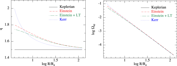
Figure 2. Orbital shear rate (left panel) and apsidal precession rate (right panel) for the Keplerian potential (black solid line), Einstein potential (red dashed line), Einstein potential with Lense–Thirring gravitomagnetic force (green long-dashed line), and from the Kerr metric (blue dotted line). Keplerian shear rate is constant, with q = 1.5, and the apsidal precession rate is zero in this case (not depicted). Curves have been evaluated for a black hole spin parameter of 0.5585. The equation for the Kerr shear parameter is taken from Gammie (2004), while the apsidal precession rate is from Kato (1990). The Einstein potential provides an accurate description of the apsidal precession rate. However, the shear parameter is only approximately correct, with errors on the order of 10%.
Download figure:
Standard image High-resolution image
Figure 3. Dimensionless growth rates,  , plotted against the warp amplitude, ψ, for different values of the viscosity parameter α, the bulk viscosity αb, and the shear parameter q. Recall that
 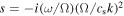 , and that perturbations grow (
 ) or decay (
 ) as
) as  . These values are calculated following the method outlined in Doğan et al. (2018) and using a code kindly provided by G. I. Ogilvie to calculate the torque coefficients (Ogilvie & Latter 2013). In the left, middle, and right panels, we plot the values for α = 0.03, 0.1, and 0.3, respectively. Black curves correspond to q = 1.5 (Keplerian), red curves to q = 1.6, and green curves to q = 1.7. Solid curves represent zero bulk viscosity, while dashed curves have αb = 0.03. Blue dotted line represents zero growth rate, marking the line of instability; for positive (and real) growth rates, the disk becomes unstable. For lower values of the disk viscosity, we see that the disk is unstable for a broad range of warp amplitude, and the growth rates increase with increasing q (although it is worth noting that this trend does not increase to very large q ≈ 2; see Doğan & Nixon 2020). For large disk viscosity, α = 0.3, we see that the disk is expected to be stable. A small level of bulk viscosity does not change the overall picture, but it can affect the exact value of the critical warp amplitudes and growth rates.
Download figure:
Standard image High-resolution imageIn numerical simulations, it is important to distinguish between physical and numerical viscosity. By physical viscosity, we refer to the Shakura & Sunyaev (1973) viscosity that we employ here to model the angular momentum transport in disks that is generally thought to arise due to disk turbulence created by the magnetorotational instability (Balbus & Hawley 1991). In different astrophysical systems, the efficiency of angular momentum transport can differ, and this is usually encapsulated in the Shakura & Sunyaev (1973) α-parameter. In fully ionized disks, α is typically found to be large (King et al. 2007; Martin et al. 2019a), but it may be lower in disks that are only partially ionized (for further discussion, see Martin et al. 2019a). Here, we employ several values of α to explore the possible range of disk evolution. This physical viscosity is implemented as a direct (Navier–Stokes) viscosity term in the simulations; see Flebbe et al. (1994) and Section 3.2.4 of Lodato & Price (2010).
Numerical solution of the equations of hydrodynamics also leads to numerical viscosity (as is the case for any numerical method; see, for example, the discussion in the Appendix of Sorathia et al. 2013). In the SPH method, numerical viscosity is added explicitly to the equations of motion, as it is required to smooth discontinuities in the velocity field. We use the standard SPH artificial viscosity terms, with a linear term (with coefficient αSPH) and a quadratic term (with coefficient βSPH). We take βSPH = 2 and allow αSPH to vary following the switch proposed by Cullen & Dehnen (2010), with a minimum value of 0.01 and maximum value of unity; for details, see Price et al. (2018). These numerical terms contribute a small level of viscosity, which when computed in terms of a Shakura & Sunyaev parameter is typically on the order of αAV ∼ 0.01, but note that this is resolution-dependent (see Equation (2) below). Ideally, this numerical viscosity should be small compared to the physical viscosity. Unfortunately this is not always the case, particularly when simulating thin disks or those with low physical viscosity. In these cases, the numerical viscosity may play a role in determining the dynamics of the instability, especially when the critical warp amplitude and growth rates of the instability depend sensitively on the value of the disk viscosity (see, e.g., Figure 3 of Doğan et al. 2018).
It is also worth noting that, in SPH simulations, the local resolution follows the local density of particles as the smoothing length (roughly the resolution lengthscale) h ∝ ρ−1/3, where ρ is the density. This is a highly useful feature of the SPH method, as it allows, for example, converging flows to be modeled with resolution that increases in regions of increasing density (e.g., gravitational fragmentation of a fluid). However, this feature also provides a challenge in modeling flows where the density drops significantly below the mean density. Such a drop in density occurs in warped disks in regions where the warp amplitude is high (Nixon & King 2012), and for an unstable disk that breaks into discrete rings, the “surface density” is significantly reduced between the rings. Therefore, it is possible that, as the disk becomes unstable, the numerical viscosity could increase and become comparable to, or larger than, the physical viscosity in the simulation. However, as the instability is stabilized by larger viscosity (Doğan et al. 2018), we expect this to have a stabilizing effect on the simulations—and thus, if instability is observed, we expect that the disk is physically unstable 6 . Such instability in low-resolution simulations may not capture the correct growth rates or extent of the instability, but at high enough resolution (such that the physical viscosity is significantly larger than the numerical viscosity) it should be possible to capture the relevant dynamics.
In numerical simulations, there will be a bulk viscosity present that was not included in, for example, Doğan et al. (2018), which employed αb = 0. The bulk viscosity has an effect on the viscosity coefficients and thus on the stability and growth rates. Lodato & Price (2010) report that the magnitude of the bulk viscosity present in an SPH simulation is  , where αAV is the shear viscosity arising from the numerical viscosity
7
. The magnitude of the shear viscosity arising from the numerical viscosity in the continuum limit is (Meru & Bate 2012)
, where αAV is the shear viscosity arising from the numerical viscosity
7
. The magnitude of the shear viscosity arising from the numerical viscosity in the continuum limit is (Meru & Bate 2012)

where  /H is the shell-averaged smoothing length per disk scale-height. For a typical value of
  and conservatively assuming
  , we have αAV ≈ 0.02 and thus
  .
.
In Figure 3, we provide the growth rates of the instability for α = 0.03, 0.1, and 0.3 (the same as the values we employ in the simulations below), with a comparison between αb = 0 and αb = 0.03. We also show the results for three different values of the disk shear, given by q = 1.5, 1.6, and 1.7. These plots show that the basic picture is unchanged; the disks are generally unstable at large warp amplitudes and small α, while generally stable at small warp amplitudes and large α (see Ogilvie 2000; Doğan et al. 2018; Doğan & Nixon 2020). However, the details are changed with the inclusion of nonzero bulk viscosity and non-Keplerian rotation. For example, the exact value of the critical warp amplitude can vary, and the growth rates at large warp amplitude can vary by factors of several.
From the above, it is clear that numerical modeling of the disk breaking instability is likely to yield subtle effects. In particular, “convergence” of the simulations with increasing spatial resolution may not be easy to achieve. As we have noted above, the critical warp amplitudes and growth rates can depend sensitively on the value of the viscosity—and thus, may depend on the resolution. With modern-day resolution, the numerical viscosity in SPH simulations is not negligible, and for disks that are sufficiently thin (H/R ≪ 0.1) to realistically model black hole accretion, we find that the numerical viscosity is typically several tens of percent of the physical viscosity. For understanding the dynamics of these disks, this is not a grave issue, as the net effect is that the simulations are somewhat more viscous than anticipated, i.e., if the numbers given above are representative, then for a physical α = 0.03, we have a total simulated viscosity of α ≈ 0.05, while for α = 0.3, we have α ≈ 0.32.
8
However, when interpreting the behavior of simulations—for example, measuring the instability growth rates and comparing them with theoretical predictions—we must be aware that the numerical terms provide an additional, resolution-dependent effect. Therefore, we anticipate that, for simulations in which the disk is “resolved” (i.e.,  ) as the resolution of the simulations is increased, we should recover the same basic dynamics (such as whether the disk is stable or unstable and whether the disk aligns to the black hole spin or not), but the precise details (such as the exact location of disk breaks and the exact growth rate in the unstable region) may vary.
9
) as the resolution of the simulations is increased, we should recover the same basic dynamics (such as whether the disk is stable or unstable and whether the disk aligns to the black hole spin or not), but the precise details (such as the exact location of disk breaks and the exact growth rate in the unstable region) may vary.
9
With these caveats in mind, we return to the focus of the paper, namely to comparing numerical simulations of warped disks with the instability of warped disks found by analytical calculations to occur at low viscosity and large warp amplitude (Ogilvie 2000; Doğan et al. 2018). We note here that the analytical work on this instability takes the form of a local linear stability analysis that makes use of the assumption that the perturbations grow (or decay) on timescales that are short compared with the evolution of the unperturbed state. In a dynamic simulation in which the background state is continuously evolving, it is likely that the instability is only realized in situations where the growth rate is sufficiently high that the instability has time to act before the disk evolves further. In this sense, the solutions presented by Doğan et al. (2018) represent necessary—but not sufficient—criteria for instability, with the sufficiency supplied by the condition that the background state evolve more slowly than the growth of unstable modes. Taking the above into account, our aims for the simulations presented in this paper are to show, in agreement with the analytical predictions of the warped disk instability, whether the following are true.
- 1.Disks with warp amplitude above the critical warp amplitude, ψ > ψc, for extended periods of time lead to instability.
- 2.Disks with ψ < ψc are stable.
- 3.The growth rate of the warp amplitude in the unstable regions follows the general trends of the predicted growth rates, i.e., the growth rates are generally higher for smaller viscosity and depend on the warp amplitude.
3. Numerical Simulations
We present three-dimensional hydrodynamical simulations of accretion disks with an imposed external torque. The fluid dynamics is modeled with the smoothed particle hydrodynamics technique (SPH; e.g., Price 2012) using the publicly available code phantom (Price et al. 2018). This code was first used to model warped disks by Lodato & Price (2010), who simulated isolated warped disks with no external torque and found excellent agreement between the disk evolution and the evolution predicted by the analytical theory of Ogilvie (1999). Motivated by the broken disks found in one-dimensional calculations of the disk structure by Nixon & King (2012), phantom was subsequently used by Nixon et al. (2012b) to model the behavior of broken disks. Disks with an external torque were modeled in the Lense–Thirring case (Nixon et al. 2012a), the circumbinary case (Nixon 2012; Nixon et al. 2013; see also Facchini et al. 2013), and the circumstellar case with a binary companion (Doğan et al. 2015). In each case, the dynamics proceeds in a similar manner; modest inclinations lead to a mild warp in the disk and alignment with the perturbing torque, while large inclinations generally lead to strong warps and often the disk breaks into discrete planes that can subsequently precess independently—this process was referred to as disk tearing by Nixon et al. (2012a).
Here, we return to the case of disks that are misaligned to the rotation of a spinning black hole and thus precess due to the Lense–Thirring effect. As discussed above, we model the central potential with the Einstein potential (e.g., Nelson & Papaloizou 2000) in order to take account of the apsidal precession of disk orbits, and we include the Lense–Thirring term through a gravitomagnetic force term (e.g., Nelson & Papaloizou 2000). For details of the implementation, see Nealon et al. (2015) and Price et al. (2018).
We take the black hole spin to be 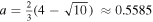 (see Lubow et al. 2002), which yields an ISCO at 4Rg, where Rg = GM/c2. The inner edge of the disk, Rin, is set to the ISCO radius, and the outer edge of the disk is initially at 120Rg. The initial disk surface density follows a power law that accounts for the zero-torque inner boundary condition as matter accretes on to the black hole, given by

where the normalization is set by the total disk mass. 10 The disk sound speed follows the locally isothermal approximation with

with the normalization fixed by the value of the disk angular semi-thickness, H/R, which is specified at Rin. For the simulations presented here, we take the power-law indices to be p = 1 and qs = 0.5, with the latter giving a constant disk angular semi-thickness. As discussed above, there are two components to the viscosity in the simulated disk: a numerical component and a physical component. For the numerical viscosity, we use the switch proposed by Cullen & Dehnen (2010) with the linear numerical viscosity coefficient αSPH allowed to vary between 0.01 and unity, and we employ a quadratic numerical viscosity with βSPH = 2. For the physical viscosity, we impose a Navier–Stokes (isotropic) viscosity of magnitude given by the Shakura-Sunyaev shear viscosity α; see Section 3.2.4 of Lodato & Price (2010), for details. Unless stated otherwise, the simulations presented below employed Np = 107 particles. The simulations are evolved to a time of 105 GM/c3, which corresponds to a factor of a few less than the Lense–Thirring (nodal) precession timescale at the outer disk radius (to ensure the outer regions are undisturbed on the timescale of the simulation) and is long enough to ensure the inner disk regions have evolved significantly (the run time is equivalent to a Lense–Thirring precession timescale at a radius of approximately 50Rg).
In the following sections, we present quantities from the simulations that require averaging over the SPH particle data. For example, the warp amplitude at each radius requires taking the radial derivative of the unit tilt (orbital angular momentum) vector for the disk. To calculate the angular momentum vector as a function of radius in the disk, we must take an average over a selection of the disk particles. For the plots presented below, we split the disk into N shells spaced logarithmically in radius. For each shell, with spherical radius rs, we average over the particles that have ∣r − rs∣ < ξ H, where H is the disk scale-height at rs. We find that choosing N = 150 and ξ = 2 serves to minimize Poisson noise from the discreteness of the particles, while not oversmoothing features in the disk.
We investigate the warped disk dynamics by varying the following parameters: we simulate disks with two thicknesses (H/R = 0.02, 0.05), three inclinations (θ = 10°, 30°, and 60°), and three values of the disk viscosity (α = 0.03, 0.1, and 0.3). This is a total of 18 simulations, so rather than provide 18 detailed sets of results, we instead focus our attention on presenting the important results. In the following subsections, we provide the results of varying each of these parameters in turn, and then also more detailed investigation into the properties of the simulations that exhibit disk tearing. We note that, in all of the simulations, we find that when the disk is stable, the solutions vary slowly with time (perhaps with some propagating waves in the cases of lowest viscosity), while for the unstable disks, the solutions are time-dependent; in this case, the disks are broken at times, and this can be long-lived, short-lived, or repeating behavior. We discuss this behavior in detail below.
3.1. Varying the Disk Thickness
The disk thickness is expected to affect the evolution of warped disks. For a disk subject to an external torque, the disk thickness affects the magnitude of the effective viscosities in the disk (which are proportional to (H/R)2) and thus affects the location at which the external torque becomes dynamically important. For example, the disk-tearing radius derived by Nixon et al. (2012a) depends on the disk thickness, with a larger extent of the disk expected to be vulnerable to instability if the disk is thinner. Another effect that arises from the disk thickness is that it alters the lengthscale on which the disk can be warped. It is not possible to bend a disk on a lengthscale shorter than ∼ H, and thus when the same torque is applied, thick disks cannot achieve as large a warp amplitude as thin disks. This implies that thick disks are less vulnerable to instability, as they are less likely to achieve a warp amplitude that is greater than the critical warp amplitude (Doğan et al. 2018). We demonstrate this by plotting (in Figure 4) the warp amplitude with radius for the simulations with α = 0.1 and the comparison between H/R = 0.02 and H/R = 0.05 (with the left-hand panel at θ = 10°, middle panel at 30°, and the right-hand panel at θ = 60°). In these cases, the disks are all coherently warped, except for the thinnest and most inclined case (H/R = 0.02, θ = 60°), which exhibits two breaks at R/Rg ≈ 8 and R/Rg ≈ 20. We note that the plots are made after a time of 5 × 10⁴ GM/c3, which is halfway through the simulation. This corresponds to a Lense–Thirring precession timescale at R ≈ 35Rg. The main results depicted by these plots are: (1) thicker disks have a peak in the warp amplitude that occurs at a smaller radius than in thinner disks (see also, for example, Kumar & Pringle 1985; Natarajan & Pringle 1998) 11 , and that (2) in general (but not always 12 ) the peak warp amplitude is higher for thinner disks and this occurs across a broad section of the disk. For the right-hand panel of Figure 4, we can see that, for the same viscosity parameter and disk inclination, the disk thickness can play a key role in determining how vulnerable the disk is to instability; this can occur both due to the increased warp amplitude and also due to the increased local viscous timescale associated with thinner disks. We also note that, for these parameters, the thinner disk (H/R = 0.02) is aligned to the black hole spin plane at the ISCO, but this is not true for the thicker case (H/R = 0.05) where, while there is a downturn in the inclination, typically the disk is still significantly misaligned at the ISCO.
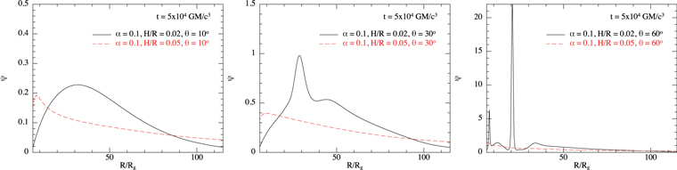
Figure 4. Warp amplitude,  , plotted against radius, R/Rg, at a time of 5 × 10⁴
GM/c3 for the simulations with α = 0.1. Each panel compares the warp amplitude in the simulation with H/R = 0.02 (black solid line) vs. the corresponding simulation with H/R = 0.05 (red dashed line), with the left, middle, and right panels respectively showing the simulation with the disk initially inclined by 10°, 30°, and 60°. In each panel, the range of warp amplitude that is plotted is varied in order to show the full extent of the solution. In each case, the peak of the warp amplitude moves to smaller radius as the disk thickness is increased, but the peak warp amplitude is typically higher when the disk is thinner. For the simulation with H/R = 0.02 and θ = 60°, there are two clear breaks in the disk at R/Rg ≈ 8 and R/Rg ≈ 20, and these are typically accompanied by deficits of warp amplitude in neighboring regions. This figure also shows that the critical warp amplitude at which the disk breaks is larger than unity for α = 0.1, as the disk remains stable for θ = 30°. For θ = 60°, the disk typically becomes unstable when ψ ≳ 2, consistent with ψc ≈ 2.25 in this case.
, plotted against radius, R/Rg, at a time of 5 × 10⁴
GM/c3 for the simulations with α = 0.1. Each panel compares the warp amplitude in the simulation with H/R = 0.02 (black solid line) vs. the corresponding simulation with H/R = 0.05 (red dashed line), with the left, middle, and right panels respectively showing the simulation with the disk initially inclined by 10°, 30°, and 60°. In each panel, the range of warp amplitude that is plotted is varied in order to show the full extent of the solution. In each case, the peak of the warp amplitude moves to smaller radius as the disk thickness is increased, but the peak warp amplitude is typically higher when the disk is thinner. For the simulation with H/R = 0.02 and θ = 60°, there are two clear breaks in the disk at R/Rg ≈ 8 and R/Rg ≈ 20, and these are typically accompanied by deficits of warp amplitude in neighboring regions. This figure also shows that the critical warp amplitude at which the disk breaks is larger than unity for α = 0.1, as the disk remains stable for θ = 30°. For θ = 60°, the disk typically becomes unstable when ψ ≳ 2, consistent with ψc ≈ 2.25 in this case.
Download figure:
Standard image High-resolution image3.2. Varying the Disk Inclination
The disk inclination has an effect on the disk evolution, as the warp amplitude is typically higher for larger inclinations. This is most easily seen for low inclinations where the evolution is essentially linear, in that the behavior can be rescaled by the inclination angle θ (see Lubow et al. 2002). However, once the inclination angle becomes large enough (typically greater than a few times H/R, which for our parameters is ≳ 10°) then the evolution becomes noticeably nonlinear in the inclination angle. This is evident in Figure 5, where the disk behavior shows a strong dependence on inclination angles between θ = 10°, 30°, and 60°. This figure shows the warp amplitudes with the same format as Figure 4, but this time for the simulations with α = 0.03. The left-hand panel shows H/R = 0.02 while the right-hand panel shows H/R = 0.05, and in both cases, the solid black, dashed red, and long-dashed green lines respectively correspond to θ = 10°, 30°, and 60°. For the lowest inclination of 10°, the warp amplitude remains low and the disk attains a coherent warped shape. This is also true for the 30° case when H/R = 0.05. For the other cases, the disk becomes sufficiently warped that the warp amplitude rises above the critical warp amplitude (Doğan et al. 2018) and the disk tears into discrete rings (the rapid change in radius of the disk orbital angular momentum vector is indicated in the warp amplitude by the sharp peaks present in Figures 4 and 5). These results reinforce the conclusion from the previous Section (3.1), as the thinner disks are subject to more vigorous tearing. These results also confirm the expectation that larger inclination results in higher warp amplitude and a higher susceptibility to instability. We note that, to first order, the Lense–Thirring precession that we simulate here has a frequency that is independent of the inclination angle (i.e., the torque is proportional to  ), while the precession frequency induced by, for example, the gravitational field of a misaligned binary system (see, e.g., Bate et al. 2000) has an angular dependence such that the frequency goes to zero at θ = 90° (the torque in this case is proportional to
  ). This means that, for disks in binary systems, the increase in warp amplitude with increasing inclination angle peaks at 45° (and also 135°), rather than at 90° in the Lense–Thirring case.
Figure 5. Warp amplitude,  , plotted against radius, R/Rg, at a time of 5 × 10⁴
GM/c3 for the simulations with α = 0.03. Each panel compares the warp amplitude in the simulation with an inclination of θ = 10° with the corresponding simulation with θ = 30° and θ = 60°, with the left (right) panel showing the simulations with disk thickness of H/R = 0.02 (0.05). Warp amplitude is typically larger for larger inclinations (and also for thinner disks; see Figure 4), and thus these disks are more likely to exhibit disk tearing. We note that, for α = 0.03, the critical warp amplitude is ψc ≈ 0.5.
, plotted against radius, R/Rg, at a time of 5 × 10⁴
GM/c3 for the simulations with α = 0.03. Each panel compares the warp amplitude in the simulation with an inclination of θ = 10° with the corresponding simulation with θ = 30° and θ = 60°, with the left (right) panel showing the simulations with disk thickness of H/R = 0.02 (0.05). Warp amplitude is typically larger for larger inclinations (and also for thinner disks; see Figure 4), and thus these disks are more likely to exhibit disk tearing. We note that, for α = 0.03, the critical warp amplitude is ψc ≈ 0.5.
Download figure:
Standard image High-resolution image3.3. Varying the Disk Viscosity
The disk viscosity parameter α plays a crucial role in the dynamics of warped disks. For α < H/R, the disk response to warping is to propagate bending waves, while for α > H/R, the disk responds by diffusing the warp (Papaloizou & Pringle 1983). In the diffusive case, which we focus on here (although note that some of our simulations are potentially wavelike, with α slightly smaller than H/R), the exact value of α plays two distinct roles in the dynamics.
The first role is that the torque coefficients for modest warp amplitudes vary with α. In the limit of small warps and low α, the usual “planar” viscosity is proportional to α, while the “vertical” viscosity is proportional to 1/α (Papaloizou & Pringle 1983). 13 Thus, for small values of α, there is a significant discrepancy between the timescales associated with the disk resisting a warp by attempting to straighten itself (governed by the vertical viscosity) and the timescale on which mass flows inward through the disk (governed principally by the planar viscosity). However, when α is large and approaches unity, these timescales become comparable. This means that large α makes it difficult to break a disk. This is because, in this case, the timescale on which the disk can internally rearrange itself, and potentially locally flatten the disk into two (or more) distinct planar regions, is similar to the timescale on which matter flows from one region of the disk to another; this latter effect can keep the disk as a coherent whole. In contrast, for smaller α, the radial communication in the disk can be severely restricted at large warp amplitudes, allowing discrete parts of the disk to behave independently; for further discussion, see Nixon & King (2012).
The second role that the disk viscosity plays in warped disk dynamics is more subtle. Ogilvie (1999) showed that the torque coefficients vary as a function of the warp amplitude in the disk, and that the way in which they vary also depends on α. Ogilvie (2000) showed that the variation in torque coefficients with warp amplitude causes an instability, and Doğan et al. (2018) and Doğan & Nixon (2020) explored this instability and connected it with the disk breaking/tearing that had been found in numerical simulations. These analyses show that the instability is generally more vigorous (i.e., it exhibits lower critical warp amplitudes and higher growth rates) for lower values of α.
In Figure 6, we show the effect of varying the value of α in the simulations. In the left-hand panel, we show the simulations with H/R = 0.02 and θ = 30° for α = 0.03, 0.1, and 0.3. In this case, we can clearly see the nonlinear effect of changing the disk viscosity on the disk warp. For the highest value of α, the disk exhibits a smooth warped shape with a peak at R/Rg ≈ 30. As α is decreased, the general shape across most of the disk remains the same and the peak warp amplitude occurs in a similar radial location. However, for lower α, the peak warp amplitude grows. This is a modest increase when α varies from 0.3 to 0.1, but reducing further to α = 0.03 renders the disk unstable and the peak warp amplitude increases sharply because of this. In the right-hand panel, we show the simulations with H/R = 0.05 and θ = 30° for the same range of α. In this case, none of the simulations reach the critical warp amplitude and they all remain stable. The peak warp amplitude moves inward slightly when α is decreased from 0.3 to 0.1 (see also, e.g., Kumar & Pringle 1985; Natarajan & Pringle 1998). These simulation results confirm the general expectation from Doğan et al. (2018) that lower α is more likely to lead to instability. It is worth reminding the reader here that the values of viscosity here are the values for the physical viscosity term in the simulations, and that the total viscosity present also includes the numerical viscosity that we discussed in detail in Section 2.
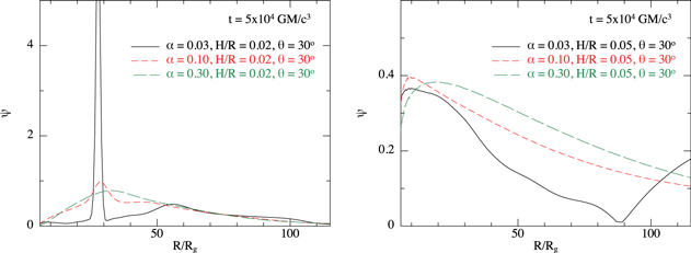
Figure 6. Warp amplitude,  , plotted against radius, R/Rg, at a time of 5 × 10⁴
GM/c3 for the simulations with θ = 30°. Each panel compares the warp amplitude in the simulations with varying values of the Shakura–Sunyaev viscosity parameter of α = 0.03, 0.1, and 0.3. Left-hand panel shows the results for the thinner case of H/R = 0.02. Right-hand panel shows the thicker case of H/R = 0.05. Left-hand panel shows that decreasing the viscosity can destabilize the disk, with the peak warp amplitude increasing until it becomes larger than the critical value. The warp amplitude at R ≈ 30Rg in the higher-viscosity cases is ≈ 0.5–1. For α = 0.03, the critical warp amplitude ψc ≈ 0.5, and thus the lower-viscosity case becomes unstable when ψ ≳ ψc as expected. Right-hand panel shows that, for stable disks, as the viscosity is decreased, the solutions can transition from diffusive to wavelike in character, as shown by Papaloizou & Pringle (1983).
, plotted against radius, R/Rg, at a time of 5 × 10⁴
GM/c3 for the simulations with θ = 30°. Each panel compares the warp amplitude in the simulations with varying values of the Shakura–Sunyaev viscosity parameter of α = 0.03, 0.1, and 0.3. Left-hand panel shows the results for the thinner case of H/R = 0.02. Right-hand panel shows the thicker case of H/R = 0.05. Left-hand panel shows that decreasing the viscosity can destabilize the disk, with the peak warp amplitude increasing until it becomes larger than the critical value. The warp amplitude at R ≈ 30Rg in the higher-viscosity cases is ≈ 0.5–1. For α = 0.03, the critical warp amplitude ψc ≈ 0.5, and thus the lower-viscosity case becomes unstable when ψ ≳ ψc as expected. Right-hand panel shows that, for stable disks, as the viscosity is decreased, the solutions can transition from diffusive to wavelike in character, as shown by Papaloizou & Pringle (1983).
Download figure:
Standard image High-resolution imageIt is also worth noting that we detect the presence of propagating waves in the simulations with α = 0.03 and H/R = 0.05 (i.e., with α ≲ H/R; see the low-amplitude waves in the warp amplitude at 30 ≲ R/Rg ≲ 80 and the upturn in warp amplitude at R/Rg ≳ 90 in the right-hand panel of Figure 6), but that these effects are noticeably reduced by the time α ≳ H/R (e.g., comparing the results with α = 0.03 and H/R = 0.02 to those with α = 0.1 and H/R = 0.05). This suggests that the transition from wavelike to diffusive as α is increased from below to above H/R may be quite sharply focused around α = H/R (see Martin et al. 2019b). This is an interesting question that warrants a focused investigation in the future.
3.4. Disk Tearing
In this subsection, we take a more detailed look at the properties of the simulated disks in which instability occurs. The simulations that exhibit clear disk tearing, and thus which we analyze in this section, are the following:
For these simulations, we note that B is the same as A, but at higher inclination. C is the same as B, but with a thicker disk. Finally, D is the same as B, but with a higher viscosity. One of the other simulations, with α = 0.03, H/R = 0.05, θ = 30°, shows an early break, which subsequently decays after propagating outward through the disk, so we do not include this in the analysis. We also find instability in the case of

As this case is anomalous from the point of view of the local stability analysis presented by Doğan et al. (2018), we discuss it separately in Section 3.5 below. The remaining simulations all warp in response to Lense–Thirring precession, but do not exhibit any instability.
We discuss in turn each of the simulations that show clear examples of disk-tearing behavior (listed A–E above). In each case, we identify two regions of the disk that exhibit a disk break caused by disk tearing. We look for clean examples where the disk is coherent beforehand and results in a single clear break (at least locally to that patch of the disk). For example, we have not chosen regions where a peak in warp amplitude ultimately splits into several distinct breaks, nor where the break occurs in a region where there is already a complex shape to the warp amplitude. In such regions, we expect the effects of different growing modes would complicate matters and make our analysis less clear. For the two breaks examined, in each case we measure the radial range (R1, R2) within which the peak of the warp amplitude resides while the peak warp amplitude grows from ψ0 at time t0 to ψ1 at time t1. 14 We then calculate the time evolution of the peak warp amplitude in this region ψp(t). In unstable regions, we expect the warp amplitude to grow as

where Ω is the orbital frequency, H ≡ cs/Ω, k is the wavenumber, and  is the dimensionless growth rate of the instability. In each unstable case, we find that the evolution of the peak warp amplitude with time is approximately exponential while the peak warp amplitude is in the range 2.5–4. (In some cases, the exponential growth starts at lower warp amplitude, and in others cases, it continues to larger warp amplitudes. However, we find this range can be consistently applied to most of our cases; when we use a different range, we note it below.) To estimate the growth rate, we rearrange (5) to give

where Δt = t1 − t0 is the time taken to grow from ψ0 = 2.5 to ψ1 = 4. We find that, in each case, the peak of the warp amplitude does not move significantly while the amplitude grows between these two bounds, allowing us to use a single value for Ω, which for the Einstein potential we employ is given by

Ideally, we would also like to measure the wavenumber, k, from the simulations so that we could compare the value of the dimensionless growth rate directly to the predicted value. However, there does not appear to be an accurate way to measure this directly from the simulation data. Future simulations that insert a growing mode with a single, well-defined value for k would be desirable. In the dynamic simulations we present here, it is likely that there is significant power at a range of wavenumbers. In this case, we can expect growth to be slower initially, until sufficient power is in the fastest-growing modes. For the mode to fit in the disk (recall that we cannot bend the disk on scales ≲ H), we must have Hk ≲ 1 (Ogilvie 2000), so we can expect the fastest-growing modes to appear with Hk less than, but not much less than, unity. However, to be consistent, we report the values of  that can be measured from the simulation data.
For simulation A with α = 0.03, H/R = 0.02, and θ = 30°, we find that the warp amplitude in the inner disk regions rapidly grows to greater than the critical value for R ≲ 15 Rg (which for this viscosity is ψc ≈ 0.5). This inner region breaks into multiple rings, starting from the inner parts and ending at ≈ 30 Rg. Outside of this region, ψ remains below the critical value at all times, and no breaks are observed in this region. For this simulation, we analyze two clear breaks. The first break occurs between R ≈ 12–18 Rg, with a peak in the warp amplitude at Rp ≈ 15Rg while the warp amplitude is growing from ψ0 = 2.5 to ψ1 = 4. The second break forms an initial peak in the warp amplitude at R ≈ 20Rg, and by the time the peak warp amplitude is ≈ 2, the peak has settled at a radius of Rp ≈ 27 Rg. For the first break, we measure Δt ≈ 1500 (in units of GM/c3), and with the peak at Rp ≈ 15Rg we have Ω ≈ 0.02. This yields χ ≈ 0.015. For the second peak, we have Δt ≈ 4000, Rp ≈ 27Rg, Ω ≈ 8 × 10⁻³, and therefore χ ≈ 0.015. This means that, when scaled to the local dynamical time, the growth rate was approximately the same in both cases, as expected. In this simulation, we expect the dimensionless growth rate to be in the range of 0.2–0.5 (see Figures 2 and 3). If  , this would imply k−1 ≈ (3–5)H, which seems reasonable, but we also note that it is likely that the total level of viscosity in the simulation is slightly higher than α = 0.03 (see discussion in Section 2) and thus we would expect the growth rate to be reduced somewhat (i.e., if α ≈ 0.05, then the predicted dimensionless growth rate implies k−1 ≈ (2–3)H).
For simulation B, with α = 0.03, H/R = 0.02, and θ = 60°, we analyze two breaks in the disk, with the first occurring at Rp ≈ 24 Rg and the second beginning at R ≈ 30Rg and settling into a strong peak at Rp ≈ 40 Rg. For the first break, we measure Δt ≈ 1650, and with the peak at Rp ≈ 24Rg we have Ω ≈ 0.01. This yields χ ≈ 0.03. For the second peak, we have Δt ≈ 5400, Rp ≈ 40Rg, Ω ≈ 4 × 10⁻³, and therefore χ ≈ 0.02. As before, when scaled to the local dynamical timescale, the growth rate in the unstable region is similar between the two breaks in the same disk, and they are also similar to the previous simulation that has the same α value.
For simulation C, with α = 0.03, H/R = 0.05, and θ = 60°, we also analyze two breaks in the disk. The first break occurs between R ≈ 20 − 30 Rg, with the peak typically at Rp ≈ 25 Rg. The second break occurs between R ≈ 30–50 Rg, with the peak typically at Rp ≈ 45 Rg. For the first break, we measure Δt ≈ 2400, and with the peak at Rp ≈ 25Rg we have Ω ≈ 9 × 10⁻³. This yields χ ≈ 0.02. For the second peak, we note that the growth in warp amplitude slows appreciably for ψ ≳ 3.5, but is approximately exponential between ψ = 2.5 and ψ = 3.5, so in this instance, we explore this range. Here, we have Δt ≈ 4000, Rp ≈ 45Rg, Ω ≈ 3.5 × 10⁻³, and therefore χ ≈ 0.025. These values are similar to those of the previous two simulations. It is worth noting that this simulation is of a thicker disk with H/R = 0.05, and in this case, the radial extent of the peak of the warp amplitude is broader than in the thinner disk simulations, by a factor of approximately 2.5, which demonstrates that the break in the disk occurs across a radial length scale of a few H independent of the value of H/R.
For simulation D, with α = 0.1, H/R = 0.02, and θ = 60°, we again analyze two breaks in the disk, with the first occurring at Rp ≈ 22 Rg and the second occurring at Rp ≈ 37Rg. For the first break, we measure Δt ≈ 1500, and with the peak at Rp ≈ 22Rg we have Ω ≈ 0.01. This yields χ ≈ 0.03. For the second peak, we have Δt ≈ 5000, Rp ≈ 37Rg, Ω ≈ 5 × 10⁻³, and therefore χ ≈ 0.02. Therefore, we find that the growth rates in this case, with α = 0.1, are similar to the growth rates found for α = 0.03. The predictions from the stability analysis suggest that the growth should be slower in this case. This may indicate that, for the lower-viscosity simulations (α = 0.03), the numerical viscosity is impeding the growth rate somewhat. Alternatively, it might be that initially growth occurs for small k (on large spatial scales), and thus the growth is slow until enough power is transferred into large k modes (smaller length scales), at which point the instability is sufficiently rapid that the timescale is essentially independent of disk parameters once the disk becomes unstable. We note that χ ≈ 0.02 implies that the instability growth timescale is ∼ 50/Ω (i.e., several orbits). It seems unreasonable to expect the instability to grow faster than this. We speculate that this second reason is what is occurring in the simulations, as we find that analyses of two of the breaks in the simulation with α = 0.1, H/R = 0.02, and θ = 60°, when performed at a resolution corresponding to Np = 106, both also yield χ ≈ 0.02, hinting that the growth rate (which encompasses the wavenumber of the fastest-growing mode) may not depend strongly on resolution.
Finally, we also note that simulation C, with α = 0.03, H/R = 0.05, and θ = 60°, performed at a resolution corresponding to Np = 106, showed some interesting dynamics that was not present in any of the other simulations. In this simulation, the peak of the warp amplitude is concentrated at small radii. There are two additional peaks of warp amplitude, which occur at larger radii. In the Np = 107 simulation, these peaks at larger radii are resolved into breaks that then alter the inner disk evolution, while in the Np = 106 case, the outer disk remained coherent. This allowed the inner regions, on longer timescales, to develop a break near the inner edge, which is quickly accreted. This process repeats with the innermost ring being broken off; it subsequently precesses, and it is then accreted. It is possible that, for the right combination of parameters and variation of those parameters with radius, that this evolution could manifest in a physical disk. For example, if the disk angular semi-thickness were a slowly increasing function of radius, then the disk may only be unstable near the inner disk edge (and this could remain so as resolution is increased). We discuss this manifestation of the disk-tearing dynamics, as well as the implications this may have for the observational properties of these disks, in more detail in Raj & Nixon (2021).
3.5. Instability at High Viscosity
We noted above that simulation E, with α = 0.3, H/R = 0.02, and θ = 60°, showed instability. This was not expected, as the local stability analysis of the warped disk equations suggests that the disk is stable for any value of the warp amplitude at this high of a viscosity. However, instability in this case had previously been reported by Nixon & King (2012) for disks subject to the Lense–Thirring precession, with those authors using a 1D ring code to evolve the warped disk evolution equations. In this case, Nixon & King (2012) showed that the disk can break into two distinct planes for α ≈ 0.2–0.3. They present evolution that is distinct from the evolution presented by most hydrodynamical simulations, in that the breaks manifest as a sharp variation in the disk tilt, while the breaks in most hydrodynamical simulations manifest (at least initially) as a sharp variation in the disk twist. Here, we find that, for α = 0.3, the break in the disk forms with a large variation in the disk tilt, consistent with the results in Nixon & King (2012).
For comparison with the growth rates reported above, we again analyze two breaks in the disk for this simulation with α = 0.3. The first break occurs at Rp ≈ 14 Rg, and the second at Rp ≈ 18Rg. For the first break, we measure Δt ≈ 950, and with the peak at Rp ≈ 14Rg we have Ω ≈ 0.02. This yields χ ≈ 0.02. For the second peak, we have Δt ≈ 1250, Rp ≈ 18Rg, Ω ≈ 0.015, and therefore χ ≈ 0.025. Therefore, we find that the growth rates in this case, with α = 0.3, are similar to the growth rates found for the lower α cases.
There are several possibilities for why the simulated disk with α = 0.3 may be unstable, contrary to the prediction of the local stability analysis. It is possible, although we consider it unlikely, that there exists an island of instability at high α for some values of the shear rate q and bulk viscosity αb that was not revealed in the analyses presented in Doğan et al. (2018) and Doğan & Nixon (2020). It is also possible that the disk tearing presented in these simulations is a numerical artifact, but again we consider this unlikely, given the broad range of codes and methods that have now reported such behavior in strongly warped disks. Instead, we speculate that the answer is related to the applicability of the warped disk equations (in particular, the accuracy of calculating the torque coefficients) and/or the local stability analysis at the extremes of the parameter space. Here, we have large viscosity and large warp amplitudes, and the disk structure is strongly affected by the external torque. It seems possible that one or more of the assumptions of the theory of warped disks could be violated, or that nonlocal effects become important. For example, as discussed by Nixon & King (2012), the torques responsible for holding the disk together generally weaken with increasing warp amplitude. This is due in part to the drop in surface density in the region of large warp amplitude. Once the surface density has dropped sufficiently far, it may be that there is simply not a strong enough torque left to hold the disk together in that region. If the stability of the disk is dependent on such a process, in which the local mass is slowly reduced over time, this may not be captured by a local stability analysis that assumes a stable background state.
4. Conclusions
We have presented and discussed the results of numerical simulations of disks that are warped by the Lense–Thirring effect from a spinning black hole. In general, we find that the results of our simulations (Section 3) are consistent with the predictions of the local stability analysis of the warped disk equations (Doğan et al. 2018). We confirm that disk tearing occurs preferentially in thin, low-viscosity, and highly inclined disks. Thin and highly inclined disks are more likely to yield large warp amplitudes, and low-viscosity disks are generally expected to become unstable at lower warp amplitudes. We show that instability arises in the simulated disks at higher values of the warp amplitude for larger viscosity parameters, and the critical warp amplitudes are commensurate with the predicted values. We also find that the growth rates of the instability are consistent with the predicted growth rates, assuming that the growing modes have wavenumbers, k, with kH ∼ 0.3 − 0.5. We also find some unexpected results. In particular, we found instability for a simulation with α = 0.3 (case E). In this case, the instability manifests with a sharp change in the disk tilt, rather than the disk twist, as previously found for similar high-viscosity cases by Nixon & King (2012) using a 1D ring code approach. This suggests that there is a difference between the dynamics in numerical simulations that include a strong external torque to provide the precession of disk orbits versus the dynamics predicted by a local stability analysis of the warped disks equations that do not include the external torque, with which Doğan et al. (2018) find that such large α value should be stable. We note that we do find that the results of the simulations vary somewhat with increasing resolution; typically, we find that the results for stable disks are converged for the bulk of the disk, with small differences near the inner edge where the density and thus resolution are lower, but we do find that higher-resolution simulations exhibit more disk breaks that are sharper (i.e., have a larger peak warp amplitude; see Appendix). We attribute this to the increase in spatial resolution, which allows smaller physical features to be resolved in the simulations, and to the decreasing influence of numerical viscosity at higher resolution. As we listed at the end of Section 2, here we have aimed to verify three propositions:
- 1.Disks with warp amplitude above the critical warp amplitude, ψ > ψc, for extended periods of time lead to instability.
- 2.Disks with ψ < ψc are stable.
- 3.The growth rate of the warp amplitude in the unstable regions follows the general trends of the predicted growth rates, i.e., that the growth rates are generally higher for smaller viscosity and depend on the warp amplitude.
Our simulations support (1) and (2), showing that the instability seen in the simulations is consistent with the predicted critical warp amplitudes. However, for (3), while the growth rates are consistent at the order-of-magnitude level, future simulations at higher resolution will be required in order to determine whether the growth rates vary in the predicted manner with disk parameters such as the viscosity parameter and warp amplitude. We discuss the observational implications of the disk-tearing behavior for black hole accretion in Raj & Nixon (2021).
We thank the referee for a helpful report. We thank Jim Pringle for useful comments on the manuscript. C. J. N. is supported by the Science and Technology Facilities Council (grant number ST/M005917/1). C. J. N. acknowledges funding from the European Union's Horizon 2020 research and innovation program under the Marie Skłodowska-Curie grant agreement No 823823 (Dustbusters RISE project). This research used the ALICE High Performance Computing Facility at the University of Leicester. This work was performed using the DiRAC Data Intensive service at Leicester, operated by the University of Leicester IT Services, which forms part of the STFC DiRAC HPC Facility (www.dirac.ac.uk). The equipment was funded by BEIS capital funding via STFC capital grants ST/K000373/1 and ST/R002363/1, as well as STFC DiRAC Operations grant ST/R001014/1. DiRAC is part of the National e-Infrastructure. We used splash (Price 2007) for the figures.
Appendix: Resolution
We have discussed the effects of resolution in detail in Section 2, and throughout. There are two principal effects that numerical resolution has on the results of warped disk simulations. First, higher spatial resolution allows for the formation of sharper features in the disk. For example, an underresolved region of high warp amplitude may result in the warp amplitude being underestimated and thus the disk remaining (artificially) stable when (physically) the disk should be unstable. Second, the numerical viscosity in SPH simulations is a function of the local resolution with the linear numerical viscosity proportional to the resolution lengthscale and the quadratic numerical viscosity proportional to the square of the resolution lengthscale (see Equation (2)). As the resolution is increased, the contribution to the total viscosity from the numerical viscosity decreases, and thus for a fixed physical viscosity, the total viscosity in the simulation decreases. As discussed in Section 2, we expect the magnitude of the numerical viscosity to be on the order of, but smaller than, the lowest physical viscosity we simulated (α = 0.03). Therefore, we expect the simulations with lower physical viscosity to be more strongly affected by it than the higher viscosity simulations with, say, α = 0.3. Both of these effects combine at the inner edge of the disk in SPH simulations where the surface density goes to zero at the inner boundary. Here, spatial gradients in the disk (for example, of the surface density) are typically largest and may be underresolved by the available spatial resolution, and the decreasing spatial resolution associated with the decreasing density of the disk results in an increased viscosity. As resolution is increased, the solution tends toward the expected solution (e.g., Equation (3) for the surface density of a planar disk). Finally, we also noted that, because the instability, including both the critical warp amplitude and the growth rates (for further details, see Doğan et al. 2018), depends sensitively on the viscosity parameter α, we cannot expect numerical simulations to show converged results for the precise details (e.g., the exact location at which the instability manifests) of unstable regions. To show an example of the differences in the simulation results at different resolutions, we plot the warp amplitudes for the simulations at different inclination angles with α = 0.1 and H/R = 0.02 in Figure 7, each time for different numbers of particles.
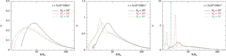
Figure 7. Warp amplitude,  , plotted against radius, R/Rg, at a time of 5 × 10⁴
GM/c3 for the simulations at different inclinations (left to right) with α = 0.1 and H/R = 0.02. Each panel compares the warp amplitude in the simulations, varying the resolution as given in the legend. Left-hand panel shows the results for an inclination of 10°. Middle panel shows an inclination of 30°. Right-hand panel shows an inclination of 60°. At low inclinations, the disk is stable, and the results are similar at a high particle number. The same is true at an inclination of 30°. At 60°, the disk is unstable for these parameters and the solutions all exhibit this, but the details are different at different resolutions, as discussed in the text.
, plotted against radius, R/Rg, at a time of 5 × 10⁴
GM/c3 for the simulations at different inclinations (left to right) with α = 0.1 and H/R = 0.02. Each panel compares the warp amplitude in the simulations, varying the resolution as given in the legend. Left-hand panel shows the results for an inclination of 10°. Middle panel shows an inclination of 30°. Right-hand panel shows an inclination of 60°. At low inclinations, the disk is stable, and the results are similar at a high particle number. The same is true at an inclination of 30°. At 60°, the disk is unstable for these parameters and the solutions all exhibit this, but the details are different at different resolutions, as discussed in the text.
Download figure:
Standard image High-resolution imageFootnotes
- 3
Note that here, for clarity, we refer to the warp amplitude using the symbol ψ. This differs from some previous works, which refer to the warp amplitude as
 due to the use of complex variables in Ogilvie (1999) in which the warp amplitude was the magnitude, , of a complex variable ψ (see Equations (44) and (45) of Ogilvie 1999). Here, we take ψ to be the warp amplitude.
 - 4
Note that, for a planar disk orbiting in, say, the x–y plane, the “surface” density is defined as the integral of the volume density with vertical height through the disk and is typically averaged in azimuth to give a single value for each radius. In a warped disk, the “surface” density retains this meaning, but now the “vertical” extent of the disk is taken normal to the local orbital plane and is a local quantity measuring the amount of mass orbiting per unit area at each radius. This is distinct from the column integral, which would measure the amount of mass along any given sight line as seen by a distant observer.
- 5
We refer the reader to Liptai & Price (2019) for a recent implementation of the SPH equations of motion in a General Relativity framework.
- 6
We note that this may not be true of simulations performed in the wavelike regime, where α < H/R. In this case, the analytical work is not as well-established as in the diffusive case, and the stability criteria is not known. Nealon et al. (2015) report numerical simulations of disks with α < H/R and find that the disk can break. However, it is not clear that the numerical viscosity was sufficiently small that these simulations were in the wavelike regime at the time instability was found. We shall return to this question in the future.
- 7
We note that an alternative method for modeling the physical viscosity in SPH simulations is to scale the numerical viscosity term to the appropriate value for a Shakura & Sunyaev (1973) viscosity (e.g., Murray 1996; Lodato & Price 2010). In this method, the bulk viscosity will always be significant compared to the shear viscosity.
- 8
It has been shown by Lodato & Price (2010) that the standard SPH numerical viscosity behaves in an “isotropic” manner. That is to say, it behaves like a Navier–Stokes viscosity, and thus one can add the viscosities in this way. This may not be true for other numerical methods.
- 9
It is also worth noting that the disk has ρ → 0 at the inner boundary. This region is therefore difficult to resolve in an SPH simulation, and is where the Lense–Thirring torque is most strongly applied. However, we remark that, while we have discussed the drawbacks of the numerical method we employ here, it is worth bearing in mind that any numerical method suffers drawbacks. For example, grid-based methods struggle to conserve angular momentum, particularly for orbits that cross the symmetry plane of the grid, which is inevitable for a warp.
- 10
As we do not take account of the gas self-gravity in these simulations, nor allow the back reaction on the black hole spin vector (from accretion or the Lense–Thirring torque), the exact value of the disk mass plays no role in the calculation.
- 11
It is worth noting that the fact that the warp amplitude can peak near the inner edge of the disk is of interest, as it allows for the possibility that the disk can produce time-dependent repeating behavior there. If the warp amplitude is maximal near the inner edge, and the value of the warp amplitude is above the critical warp amplitude there (see Doğan & Nixon 2020), then the innermost ring of the disk may tear off, precess and be rapidly accreted, and this process may repeat indefinitely (or at least until the disk conditions change, causing the warp amplitude there to evolve). We discuss one example of this from our simulations in more detail in Raj & Nixon (2021).
- 12
For example, the simulations corresponding to the left-hand panel of Figure 4 but with α = 0.03 (not depicted) show a higher peak warp amplitude in the thicker case. For these cases, the peak in the thicker case occurs at a small radius, at which the thinner disk has already aligned to the black hole spin.
- 13
Here, we have assumed that the underlying mechanism generating the viscosity is essentially isotropic, such that any shear is damped at the same rate (given by α), as might be expected when the viscosity arises due to small-scale turbulence. For a discussion of the viscosity coefficients in the case that the underlying mechanism generates an anisotropic viscosity, see Nixon (2015).
- 14
Note that, when searching for the peak warp amplitude, we find that the 150 logarithmically spaced radial points used in the previous sections to be insufficient. For these calculations, we employ a linear spaced grid with 1200 points.

