Abstract
Observations of the S stars, the cluster of young stars in the inner 0.1 pc of the Galactic center, have been crucial in providing conclusive evidence for a supermassive black hole at the center of our galaxy. Since some of the stars have orbits less than that of a typical human lifetime, it is possible to observe multiple orbits and test the weak-field regime of general relativity. Current calculations of orbits require relatively slow and expensive computations in order to perform numerical integrations for the position and momentum of each star at each observing time. In this paper, we present a computationally efficient, first-order post-Newtonian model for the astrometric and spectroscopic data gathered for the S stars. We find that future, 30 m class telescopes—and potentially even current large telescopes with very high spectroscopic resolution—may be able to detect the Shapiro effect for an S star in the next decade or so.
Original content from this work may be used under the terms of the Creative Commons Attribution 4.0 licence. Any further distribution of this work must maintain attribution to the author(s) and the title of the work, journal citation and DOI.
1. Introduction
Supermassive black holes are located at the center of most large galaxies (e.g., Kormendy & Richstone 1995; Kormendy & Ho 2013) and provide a unique environment for probing the effects of general relativity (GR). The Milky Way contains its own central black hole, Sagittarius A* (Sgr A*; McGee & Bolton 1954; Downes & Martin 1971; Lo 1989; Lo et al. 1993; Backer 1994; Genzel et al. 1994; Ghez et al. 1998; Eckart & Genzel 1999), which is surrounded by a cluster of young stars (referred to as S stars; Eckart & Genzel 1996, 1997; Ghez et al. 1998; Genzel & Eckart 1998; Eckart et al. 1999). Measuring their orbits have helped measure the ratio of the mass-to-distance ratio of Sgr A* (Genzel et al. 1996; Eckart & Genzel 1996, 1997; Genzel et al. 1997; Ghez et al. 2000, 2008; Do et al. 2013; Boehle et al. 2016).
One of the closest stars to Sgr A* is S0-2 (also known as S2; Schödel et al. 2002; Ghez et al. 2003; Gillessen et al. 2009), which has an orbital period of around 16 yr and an eccentricity of 0.88. Long-term studies of its orbit led to the first detection of gravitational effects during its 2018 periapsis—namely, gravitational redshift (GRAVITY Collaboration et al. 2018, 2019; Do et al. 2019; GRAVITY Collaboration et al. 2021, 2022a) and Schwarzschild precession (GRAVITY Collaboration et al. 2020)—in an S-star orbit. As both photometric and spectroscopic sensitivities improve and shorter-period S-star candidates are identified (e.g., Peißker et al. 2020a, 2020b), additional tools are needed to analyze and detect higher-order GR effects, such as the Shapiro delay, and additional precession due to the frame dragging and quadrupole moment of the spacetime (e.g., Wex & Kopeikin 1999; Weinberg & Milosavljevic 2004; Will 2008; Angélil et al. 2010; Merritt et al. 2010; Angélil & Saha 2014; Psaltis et al. 2016; Grould et al. 2017; Waisberg et al. 2018).
Current modeling of S-star orbits involves integrating numerically the GR equations of motion for each time step (e.g., Gillessen et al. 2017; Do et al. 2019). This method requires integrating across the span of observations using very small time steps to avoid error buildup and results in slow, expensive computations. Furthermore, the computational cost of such numerical calculations increases rapidly when using the orbits of multiple stars to jointly constrain the shared properties of the system (e.g., the black hole mass), since this involves simultaneously solving the geodesic equations for each time step for each star. This approach could become prohibitive when searching the multidimensional orbital parameter space with a statistical sampling algorithm, such as a Markov Chain Monte Carlo (MCMC), to obtain optimal solutions and quantify uncertainties in orbital parameters.
A simplification to these calculations can be introduced because of the fact that S-star orbits have pericenter distances that range from 1400 Sgr A* Schwarzschild radii to values that are larger by orders of magnitude (Gillessen et al. 2017). At such distances the orbits can be modeled as primarily Keplerian orbits with small corrections caused by GR effects. A framework for describing this behavior is through a semi-analytic post-Newtonian (PN) model, which uses traditional Keplerian orbital equations with additional terms up to some order in v/c, derived from GR equations.
Damour & Deruelle (1985, 1986, referred to hereafter as D&DI and D&DII) obtained an elegant analytic solution to the two-body problem in the first post-Newtonian order (1PN), which incorporates a variety of relativistic effects. The timing model developed by D&DII has been the workhorse for the pulsar community for many years in detecting relativistic effects (e.g., Edwards et al. 2006). It was further expanded to include second-order post-Newtonian (2PN) terms (Damour & Schafer 1988; Wex 1995).
While the D&DII analytic solution has been implemented in a timing model for fitting pulsar arrival times, the same model is not readily applicable for fitting astrometric and spectroscopic data of stars. This is because the latter relies on the Doppler shifts of absorption or emission lines in the stellar spectra as opposed to time intervals between pulses. The beauty of the analytic D&DII timing model, however, makes it possible to derive the line-of-sight velocities that correspond to a variety of time delays.
In this paper, we use the framework of the D&DI and D&DII 1PN two-body model (in harmonic coordinates) to derive a new analytic astrometric and spectroscopic model that incorporates the relativistic and astrophysical effects relevant to modeling S-star orbits.
In addition to computational efficiency, there are significant scientific advantages to our approach. In the numerical approach, all relativistic effects of the same PN order that are embedded in the geodesic equations are reported as a single observable (i.e., the position in the sky or spectroscopic line shift). In principle, the magnitudes of the individual effects can be disentangled by exploring the differences in the numerical solutions with and without each effect (Grould et al. 2017). In contrast, a PN analytic approach, such as our model, allows for calculating directly the characteristic “fingerprint” of each effect on the observables separately from the others (see Section 6), while providing a direct analytic handle of the dependence of each effect on the various parameters of the system.
The following sections present the two-body orbital equations (Section 2), the projection of those equations to the plane of the sky (Section 3), and the equations for spectroscopic effects (Section 4). We discuss the implications of the model for S-star observations in Section 6. Unless otherwise indicated, we use geometrized units, i.e., G = c = 1, where G is the gravitational constant and c is the speed of light.
2. Orbital Model
As discussed in Section 1, our model has three main components: the two-body orbital model, the astrometric model, and the spectroscopic model. Since we want to use our model to be able to fit observations of the S stars, we first identify what parameters are the observables. With telescopes, we are able to observe the projected positions of the stars, i.e., R.A. (α) and decl. (δ), and the radial velocities derived from their spectra:

where λ0 is the rest-frame wavelength of the stellar absorption or emission line used for measuring radial velocities and Δλ is the shift at time tobs between observed and rest-frame wavelengths.
Four free parameters, the orbital period (P), the total mass of the system (M), the mass ratio of the two bodies (q), and the radial eccentricity (eR ), govern the shape, period, and rate of precession of the two-body orbits.
The orientations of the orbits with respect to Earth determine the two-dimensional motions in the sky (i.e., the astrometric model) and the line-of-sight motions, which we can derive through spectroscopy. The three orientation angles, the inclination (i), argument of ascending node (Ω), initial argument of periapsis (ω0), and initial time of periapsis (or epoch of position, t0), are free parameters for our model. We must also fit the projected and line-of-sight proper motions of the Galactic center with respect to Earth (μα , μδ , μ∥).
Nineteen additional quantities (introduced in the following sections) are derived parameters that we calculate from the observed or free parameters. Table 1 in Appendix B lists all the parameters introduced in this paper with appropriate references and units. Figure 1 illustrates how the binary system orbital parameters relate to each other.

Figure 1. The binary orbital parameters in the barycenter frame of the system. The large red, precessing ellipse shows the motion of the smaller mass m2 over roughly two periods. Similarly, the smaller blue ellipse shows the motion of the larger mass m1 over the same amount of time. Dotted magenta lines mark the semimajor and semiminor axes of the ellipses for both objects around the binary barycenter, which is indicated by a black dot. Arrows between the binary barycenter and the two masses denote the distances r1 and r2 between the binary barycenter and orbiting objects. A black “x” marks the closest approach that the smaller mass m2 makes to the larger mass m1, which precesses by an angle Δθ for each orbit. The position angle, θ, is the angle formed between the periapsis point and the location of one of the masses, which are offset from each other by 180°.
Download figure:
Standard image High-resolution imageIn this section, we present the orbital equations and parameters in geometrized units.
2.1. Coordinate Systems
We use four main coordinate systems/reference frames (Figure 2), all of which are described in Edwards et al. (2006). These are the star reference frame (denoted by the subscript “star”), the binary barycenter (BB), the solar system barycenter (SSB), and the observer reference frame (“obs”). The different reference frames are necessary to define the various time delays discussed in Section 4. All celestial sky coordinates are given in the International Celestial Reference System (Luzum & Petit 2015).
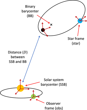
Figure 2. The relationship between the observer frame, the solar system barycenter, the binary barycenter, and the star frame, as defined in this paper. Distances and object sizes have been rescaled to show effect. The red axes for each reference frame are arbitrary to show how coordinate systems may vary from frame to frame depending on orientation.
Download figure:
Standard image High-resolution image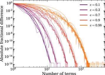
Figure 3. Convergence plots for the calculation of the position angle of orbiting objects (θ) with eccentricities of 0.1, 0.3, 0.5, 0.7, 0.9, and 0.98 for a variety of different orbital phases. With the exception of very high eccentricities, 30 terms are typically sufficient for errors of less than 10−8.
Download figure:
Standard image High-resolution imageThe times (or “clocks”) we use in this paper are directly related to the four reference frames. We define the time of emission as measured at the stellar location as tstar, the same time as measured by an observer at the binary barycenter as tBB, the time of arrival at the binary barycenter as ta,BB, the time of arrival at the solar system barycenter as tSSB, and the time of arrival recorded by the observer on Earth as tobs.
The relation between the observer light arrival time tobs and the star light emission time tstar (used for the time-dependent orbital equations in Section 2.7) is the star-frame emission time plus the sum of all time delays due to binary system motion, solar system motion, and motion between the binary barycenter and solar system barycenter/observer, i.e.,
In our model, the total binary system time delay includes the binary Roemer delay (ΔRB), binary Einstein delay (ΔEB), and binary Shapiro delay (ΔSB). The total solar-system-related time delay is the Earth Roemer delay (ΔR☉). The interstellar time delay comprises time delays due to parallax and proper motion, which is simply the Kopeikin effect (ΔKB). We provide explicit formulae for the time delays in Section 4.
Additional relations between the other time variables are as follows. The binary Einstein delay relates the star emission time to the time as measured at the binary barycenter by an inertial observer as tBB = tstar + ΔEB. The time of arrival at the binary barycenter relates to the star emission time via the binary effects, i.e., ta,BB = tstar + ΔRB + ΔEB + ΔSB. Similarly, the observer time of arrival relates to the solar system barycenter time of arrival via the solar system effects, i.e., tobs = tSSB + ΔR☉. Since the spectroscopic timing model is less sensitive than pulsar timing, we neglect interstellar delays (such as dispersion). As a result, the solar system barycenter time of arrival and binary barycenter time of arrival are related by a constant offset, which we set to zero without loss of generality.
2.2. Mass Measures
Three of the key values in describing a two-body orbital system are the total system mass and the individual masses of the two objects. We denote the component masses by m1 and m2, such that m2 ≤ m1. In the case of modeling stars orbiting a supermassive black hole, m1 is the mass of the black hole and m2 is the mass of the star. The total mass of the system is M = m1 + m2. In classical, two-body orbits, the mass ratio of the two objects,

is an important parameter that we can use to rewrite the reduced mass,

and dimensionless reduced mass (ν) as

Note that in Sgr A*–S-star systems, the mass ratios can be q ∼ 10−6–10−5. In these cases, one can take the limit of q ≪ 1, but in this paper we leave the full expressions for generality.
2.3. Period, Semimajor Axis, and Mean Motion
The easiest, most direct property to measure is the orbital period, P. With the total system mass and orbital period, we use the 1PN version of Kepler’s law (Blanchet et al. 1998, their Equation (8.6)) to calculate the center-of-mass semimajor axis, implicitly, via
Another useful related quantity is the mean motion, the constant angular speed needed for an object to complete an equivalent circular orbit. It relates to the inverse period as

2.4. Energy and Momentum
In addition to calculating the semimajor axis, aR , from P, we also fit for the eccentricity, eR . In combination with the system mass, M, and the dimensionless reduced mass, ν, these two parameters set the orbital behavior and we use them to calculate the energy and angular momentum of the system. Here, the total energy is

and the total angular momentum is
We also define the quantity K, which is the GR correction to the total angular momentum of the system, rewritten in natural units from D&DI (their Equation (4.14)) and given by
This is a particularly important quantity, as the value of K is what governs the orbital precession,

where Δθ is the angle the orbit precesses in each period (D&DI).
2.5. Other Eccentricities
While Keplerian orbits have only one effective eccentricity, eR , in GR, there are additional eccentricities that result from the curved spacetime (D&DI, their Equations (3.6b)–(c), (4.13)). In the 1PN model, these are the time eccentricity (et ; D&DI, their Equation (3.6c)),
and the angular eccentricity (eθ ; D&DI, their Equation (4.13)), which in natural units is
In some cases, the differences between the eccentricities are negligible and all eccentricity expressions give comparable answers (see Section 4 for examples). The radial eccentricity can be determined readily from observational astrometric data.
2.6. Individual Object Parameters
As noted in Section 2.3, the semimajor axis and radial eccentricity defined here are with respect to the center of mass of the system. Since observations of the S stars result in tracking the orbits of the individual stars, we need the derived parameters (i.e., the semimajor axis and radial eccentricity) that give the orbital shapes of both objects in a two-body system, which we can derive from the corresponding effective one-body parameters (i.e., aR and eR ) and the mass ratio (q).
For the more massive of the two bodies, m1, the semimajor axis of its respective orbit around the binary barycenter is

and the radial eccentricity is

(D&DI, their Equations (6.3a)–(b), in natural units and mass ratio q).
Similarly, the less massive of the two bodies, m2, follows an orbit around the binary barycenter with a semimajor axis of

and a radial eccentricity of
(D&DI, their Equations (6.3a)–(b), in natural units and mass ratio q).
2.7. Time-dependent Orbital Motion
In Sections 2.2 through 2.6, we presented the equations necessary for calculating many of the derived parameters in the model. In this section, we use those parameters to obtain the time-dependent orbital motion of the individual objects and the binary barycenter.
The heart of this time dependence comes from Kepler’s equation, which relates time eccentricity (et ), mean motion (n), mean anomaly (u), star time of emission (tstar), and epoch of position (t0) via D&DI (their Equation (3.3)):

The mean anomaly, which is the angle between the periapsis of an orbit and another position in the orbit at some time, is crucial for calculating the other values in the polar orbital equations (i.e., radius and angle). The previous equation does not have an analytical solution for u but can be solved using a fast algorithm, such as the Newton–Raphson method. Note that, unlike the time-dependent equations in the astrometric model (Section 3), which use the observer time tobs, Kepler’s equation is evaluated at the star time of emission tstar. This difference, described by Equation (2), takes into account the vacuum retardation effect for the astrometric model.
The time-dependent distances of the two orbiting bodies from the barycenter, as given in D&DI (their Equations (7.1d)–(e)), are

and

Calculating the position angle θ of the orbiting objects is somewhat more complicated. D&DI present the rather straightforward equation (their Equation (4.11b))
but using this in computations requires special care because the evaluation of the term  results in floating-point errors for the calculated value of θ around the asymptotes (i.e., u = x
π for odd x). Instead, we use a series expansion (D&DII, their Equation (17d)) of this equation (D&DI, their Equation (4.11a)), which avoids these computational issues:
results in floating-point errors for the calculated value of θ around the asymptotes (i.e., u = x
π for odd x). Instead, we use a series expansion (D&DII, their Equation (17d)) of this equation (D&DI, their Equation (4.11a)), which avoids these computational issues:

where
We performed convergence tests (Figure 3) of the series Ae (u) at different values of angular eccentricity (eθ ) and determined that only a small number of terms is needed for necessary computational accuracy, e.g., 30 terms for fractional errors of less than 10−8.
Much like the position angle θ, the argument of periapsis also precesses due to GR effects (Equation 5(c)). Given the initial argument of periapsis, the time-dependent argument of periapsis (in terms of the mean anomaly, u) is

3. Astrometric Model
In the previous section (Section 2), the 1PN orbital equations are expressed with respect to the binary barycenter. In order to model observations, however, we must transform them to a frame with respect to the plane of the sky, i.e., in terms of R.A. (α) and decl. (δ).
We make a transformation from binary barycenter motions to projected sky motions by first converting the polar binary barycentric frame (r1, r2, θ) to a Cartesian binary barycentric frame (x, y) as is typically done, i.e.,


and

We transform the positions from the Cartesian binary barycentric frame to the plane of the sky using using three angles: the inclination (i), longitude of the ascending node (Ω), and argument of periapsis (ω0). The inclination describes the tilt of the orbit with respect to the observer, while the longitude of the ascending node is the rotation of the location of the ascending node (i.e., where the orbit intersects with the reference plane) with respect to the center of mass. Similarly, the argument of periapsis is the rotation of the object point of closest approach to the center of mass in the orbital plane. See Figure 4 for a graphic depiction.

Figure 4. Diagram showing the relationship of the three angles used in the astrometric model: inclination (i), longitude of the ascending node (Ω), and argument of periapsis (ω). The angled blue ellipse shows the orbital plane, with the periapsis point marked. The gray plane is parallel to the vector pointing toward the observer and gives perspective for how the orbital plane is inclined with respect to Earth.
Download figure:
Standard image High-resolution imageWe use the Thiele–Innes constants (A, B, C, F, G, H) defined by Equations (20)–(25) in O’Neil et al. (2019) to describe this rotation:


and

The relative R.A. and decl. values (Δα and Δδ) with respect to the celestial coordinates of the binary barycenter in the sky (denoted by α0 and δ0) use combinations of these constants (as described in O’Neil et al. 2019), such that

and

where d is the distance between the solar system barycenter and the binary barycenter. These sky projection values are in units of radians.
While proper motion and parallax do fall under the category of astrometry, since they affect the observed positions of the binary system in the sky, they are calibrated out by subtracting the binary barycenter coordinates from the observed R.A. and decl. values, as done in Equations 9(k) and 9(l). The binary barycenter coordinates, α0 and δ0, change over time due to proper motion. Given some sky coordinate, ai and δi , at initial time t0, after time tobs, the new R.A. becomes

and the new decl. becomes

Parallax and proper motions still contribute to line-of-sight motions, however, and we discuss the effects on observed radial velocities in Section 4.5.
The various Newtonian and relativistic effects enter the astrometric model in two ways, via their contribution to (i) the relative positions of the stars and the black hole in the frame of the binary barycenter, and (ii) the light propagation time between the star and the observer. Indeed, Equation 8(a) for the calculation of the relative positions is written in terms of tstar, which is determined by propagation effects and is related to the time of observation tobs via Equation (2). We provide explicit equations for the various propagation effects in the following section, since we will use the same equations to derive the various spectroscopic effects.
In the astrometric model, so far we have neglected the effects of gravitational lensing of the stellar positions in the black hole spacetime. These effects have been explored, for example, in Nusser & Broadhurst (2004) and Bozza & Mancini (2012), and, albeit nondetectable with current data, might be relevant for modeling future observations (Grould et al. 2017).
4. Spectroscopic Model
As discussed in Section 1, pulsar timing models (e.g., D&DII; Edwards et al. 2006) use the time delays between emission and observation of pulses from binary pulsar systems to fit for the orbital parameters. With the S stars, we have both astrometric as well as spectroscopic data. In the previous section, we presented the equations we use to model the astrometric data. In this section, we present new line-of-sight velocity equations, which we derive from the time delay equations given in Edwards et al. (2006).
Our spectroscopic model incorporates five timing effects (presented in the following subsections): the binary Roemer effect (Section 4.1), the periastron precession (Section 4.2), the binary Einstein effect (Section 4.3), the binary Shapiro effect (Section 4.4), and the Earth Roemer effect (Section 4.6). We also derive velocity equations for the Kopeikin effect (Section 4.5) and the solar Shapiro effect (which we do not report here for brevity) to check their magnitudes and confirm that they are negligible. This allows us to omit other timing delays listed in Edwards et al. (2006) that are caused by Earth, the solar system, interstellar space, as well as higher-order GR effects, such as frame dragging, quadrupole moment, and additional 2PN terms as described in Angélil et al. (2010).
All time derivatives listed in this section are with respect to the observer time (tobs), or the arrival time of the light from the star as seen by the observer.
4.1. Binary Roemer Effect
The binary Roemer delay component (i.e., the component of the Roemer delay that pertains only to the movement of the star around the binary barycenter) is denoted by ΔRB. It is simply the light travel time for the line-of-sight distance across the orbit divided by the speed of light (i.e.,  ). Adapting notation from both D&DII and Edwards et al. (2006), we calculate the binary Roemer delay as
Taking the time derivative of Equation 10(a) gives the equation of radial velocity resulting from the binary Roemer effect:
where du/dt is derived from Kepler’s equation (Equation 8(a)) such that

The additional term vω results from the time dependence of the argument of periastron, ω. It is known as the periastron precession, which we introduce below.
4.2. Periastron Precession
Periastron precession is a first-order GR effect that causes the orbit of an object to shift or rotate around its pericenter over time. As the location of periapsis advances around the binary barycenter, the slight change in direction from a regular elliptical orbit results in an observed, line-of-sight velocity boost for the orbiting object. The d ω/dt term in the time derivative of the binary Roemer delay (Equation 10(b)) describes this spectroscopic effect:
The time derivative of the argument of periastron (d ω/dt) relates to the time derivative of the mean anomaly du/dt (Equation 10(c)) by
where K is again the dimensionless parameter related to the total momentum of the system and determines the amount of orbital precession (Equations 5(c)–5(d) and 8(g)).
4.3. Binary Einstein Effect
The binary Einstein delay (ΔEB) accounts for the difference between the star time of emission (tstar) and the binary barycenter time (tBB), which occurs due to both gravitational redshift (from GR) and time dilation (from special relativity). We write the binary Einstein time delay as

where m1 is the companion mass to the orbiting star (since we define m1 ≥ m2). The derivative of this time delay, then, is simply
which, when we substitute in the expression for du/dt (Equation 10(c)), becomes
In the case of a circular orbit, Equation 12(c) results in a null effect, even though gravitational and relativistic Doppler effects are still present. The reason is that this equation only describes the change in the combined wavelength shift along an eccentric orbit introduced by the changing separation and velocity magnitude. The baseline effect is absorbed into the systemic radial velocity of the object, i.e., the line-of-sight proper motion (μ∥), which is a free parameter, and can be trivially obtained in post-processing.
4.4. Binary Shapiro Effect
The binary Shapiro delay (ΔSB) describes the GR effect introduced when light from one of the bodies in the model passes through the gravitational well of the other. We rewrite Equation (73) from Edwards et al. (2006) in geometrized units as
where the usage of e without a subscript indicates that any eccentricity (i.e., eR , eθ , et ) may be used, as the difference is negligible. This results from the fact that the expressions for the three eccentricities differ at the ∼1/c2 order, which we omit in the 1PN limit since they already multiply a term of the same order.
The time derivative of the binary Shapiro delay (ΔSB) gives the binary Shapiro effect for spectroscopic measurements:
where we have introduced the symbol  , i.e.,
4.5. Kopeikin Effect
The Kopeikin effect combines spectroscopic contributions from both proper motion of the binary system and the parallax as seen from Earth. As discussed in Section 3, this is an astrometric effect, as well, but is calibrated out by subtracting the binary barycenter location from all observed positions of the two bodies for each time step or observation.
We base our definition of the Kopeikin effect (ΔKB) on Sections 2.7.1 and 2.7.2 in Edwards et al. (2006), where it is broken into three components (Edwards et al. 2006, their Equation (72)):

Here, ΔSR is caused by changes in the viewing angle geometry due to the proper motion, ΔAOP is due to the annual orbital parallax, and ΔOP is due to the orbital parallax (the orbital equivalent of the Shklovskii effect). These three components, rewritten in geometrized units from Edwards et al. (2006, their Equations (73)–(75)), are

and
where C and S are given by Equations (65) and (66) in Edwards et al. (2006) and  .
.
The annual orbital parallax and orbital parallax distances (to the binary barycenter) are approximately equal such that d ≈ dAOP ≈ dOP. As with the previous effects, the total Kopeikin effect is simply the time derivative of the above equations:

where

and
Here, the symbols  and
and  are defined as
and
The time derivatives of the expressions for C and S are
and
4.6. Earth Roemer Effect
The Earth Roemer effect is analogous to the binary Roemer effect (Section 4.1), except that the changes in light travel time are due to the motion of the Earth around the solar system barycenter. We define the Earth-motion Roemer delay component using similar notation to Equations (13)–(16) in Edwards et al. (2006):

where r ⊕ is the vector from the solar system barycenter to the Earth:
and  is the unit vector between the binary barycenter and the observer:
The binary barycenter–observer unit vector ( ) breaks down to the primary component (
 ), which is the initial unit vector between the observer and the binary barycenter (in celestial coordinates), i.e.,
and the shift in the binary barycenter position over time due to proper motion (μα , μδ , μ∥) of the binary system. While the line-of-sight proper motion, μ∥, is one of the free parameters for the model, the transverse proper motion, μ⊥, depends on the R.A. and decl. proper motions, μα and μδ . We define the transverse proper motion as

where the projected R.A. and decl. vectors  and
and  are given by Edwards et al. (2006, their Equations (17)–(18)):
and
The Earth Roemer effect is the time derivative of the Earth Roemer delay (Equation 15(a)), such that

where the symbols  ,
,  ,
,  , and
, and  are shorthand for


and

5. Summary of Model
Having presented all of the equations and parameters we use in our analytic, 1PN model for S stars, we summarize in Figure 5 the steps one should take to implement it.

Figure 5. Steps for implementing the new 1PN astrometric and spectroscopic model presented in this paper.
Download figure:
Standard image High-resolution imageThe Earth Roemer and Kopeikin effects both depend on the position of the Earth around the Sun, and so to calculate them we must use Earth ephemerides. For the time derivatives of any values that use these data, we use three-point midpoint differentiation.
6. Spectroscopic Effects of S Stars
6.1. Magnitude of Spectroscopic Effects
Due to the exquisite accuracy of pulsar observations, pulsar timing models must incorporate numerous time delays in addition to the geometric and relativistic effects from the binary system. Such effects include atmospheric delays, dispersion from both the interplanetary medium and interstellar medium, frequency-dependent delays, and gravitational effects from many bodies in our solar system, namely Venus, Jupiter, Saturn, Uranus, and Neptune (in addition to the Sun).
Timing models for spectroscopic observations of S stars, on the other hand, do not require the same accuracy. The current sensitivity level for Doppler shifts on the instruments capable of observing the S stars (i.e., Keck and the Very Large Telescope) are around 10 km s−1 (Thatte et al. 1998; Martin et al. 2018), and upcoming ground-based 25–40 m extremely large telescopes (ELTs) are anticipated to have velocity sensitivities of around 1 km s−1 (e.g., Mawet et al. 2019; Marconi et al. 2021). As a result, we may neglect timing effects that are significantly smaller than predicted ELT-class sensitivities. Note that the ELT-class sensitivities have been estimated for stars down to ∼19 mid-infrared magnitude, but will depend on the actual properties of stars with smaller orbital separations that may be discovered in the future.
In considering the possibility of detecting higher-order GR effects, it is useful to consider the order-of-magnitude strengths of the spectroscopic effects described in Section 4. We derived scaling equations for the six velocity components of the spectroscopic model and present them in Appendix A.
Using these scaling relations, we show in Figure 6 the relative strengths of the binary Roemer effect, binary Einstein effect, periastron precession, binary Shapiro effect, Earth Roemer effect, and Kopeikin effect for orbital periods that range from 0.5 to 500 yr with a fixed system mass and two-body mass ratio that is characteristic of Sgr A* and the S stars. The widths of the bands result from a range of eccentricities, e = 0.7–0.98, with the smaller effects corresponding to lower eccentricities.

Figure 6. Absolute magnitudes of characteristic contributions to the radial-velocity corrections in spectroscopic models of stellar orbits around Sgr A* introduced by the various Newtonian and PN effects. Each shaded area corresponds to orbital eccentricities in the range 0.7–0.98, with lower limits corresponding to e = 0.7 and upper limits corresponding to e = 0.98. The orientation angles of the orbits are assumed to be those of the S0-2 star. Horizontal dashed lines show the current measurement limits for VLT/Keck observations as well as the expected limits for an ELT-class telescope. We see that while the binary Roemer effect (far left, solid red band) is the dominant velocity contribution, the three GR effects—binary Einstein effect, periastron precession, and binary Shapiro effect—rapidly increase at smaller semimajor axes/orbital periods. The periastron precession effect (second from right, purple band) has the strongest dependence on eccentricity and spans four orders of magnitude, overlapping with the binary Einstein effect (second from left, yellow band) and Shapiro effect (far right, light blue band), which span one and three orders of magnitude, respectively. While the binary system spectroscopic effects—binary Roemer, binary Einstein, periastron precession, and binary Shapiro—decrease for larger orbital separations (semimajor axes), the Kopeikin effect describes velocity contributions due to parallax and proper motions that are due to the movement of the observer and, as such, increases for larger orbital separations.
Download figure:
Standard image High-resolution imageIn this plot, we see that the absolute magnitudes of the spectroscopic effects differ greatly from each other: while the binary Roemer effect results in velocities that range from 102–105 km s−1, the Kopeikin effect has velocities that span 10−4–10−2 km s−1. The binary Einstein, periastron precession, and binary Shapiro effects fall between these two extremes, with Doppler effect ranges of 100−103 km s−1, 10−3–104 km s−1, and 10−3–102 km s−1, respectively.
Another notable aspect of Figure 6 is the difference in the slopes of the various spectroscopic effects. As a purely geometric phenomenon, wavelength shifts introduced by the binary Roemer effect scale as  , growing larger with smaller semimajor axes. The magnitudes of the periastron precession and binary Shapiro effects also increase with smaller semimajor axes and periods, although they do so much more rapidly (
 ). This is because of the steeper scaling of the PN corrections with orbital separation. Similarly, the binary Einstein effect lies in between these scalings (
 ). The Kopeikin effect, on the other hand, is not a GR effect. Rather, it describes the radial-velocity contributions from the parallax and proper motions of the binary system. As a result, since there is more time for parallactic effects and proper motions to affect observations for any given orbit, the magnitude of the corresponding Doppler effect grows as the orbital period increases (Δλ/λ ∼ aR
∼ P2/3). The magnitude of the Earth Roemer spectroscopic effect is independent of binary orbital period and, as such, has a constant magnitude of ∼30 km s−1.
). The Kopeikin effect, on the other hand, is not a GR effect. Rather, it describes the radial-velocity contributions from the parallax and proper motions of the binary system. As a result, since there is more time for parallactic effects and proper motions to affect observations for any given orbit, the magnitude of the corresponding Doppler effect grows as the orbital period increases (Δλ/λ ∼ aR
∼ P2/3). The magnitude of the Earth Roemer spectroscopic effect is independent of binary orbital period and, as such, has a constant magnitude of ∼30 km s−1.
One last property to note is the effect of eccentricity on the magnitudes of the spectroscopic effects. For any fixed orbital period, the binary Roemer effect has a span of two orders of magnitude, the binary Einstein effect ranges around two orders, the periastron precession stretches almost four orders of magnitude, the binary Shapiro effect extends over three orders, and the Kopeikin effect spans one order. The three GR effects—binary Einstein effect, periastron precession, and binary Shapiro effect—are most dramatically influenced by changes in eccentricity. Higher eccentricities bring orbiting stars increasingly closer to the central black hole, resulting in higher angular momenta of the system (Equation 5(b)–5(c)) and larger amounts of orbital precession (Δθ), as well as greater Doppler contributions from the periastron precession effect. Similarly, the smaller the periapsis distance is (due to higher eccentricities), the closer the light from orbiting stars must pass through the potential well of the central black hole, which also increases the binary Shapiro effect.
We can reach several significant conclusions from Figure 6. First, based on the expected sensitivities of ELT-class telescopes of ∼1 km s−1, we find that the binary Shapiro effect should be detectable by these telescopes through spectroscopic observations alone during the next S0-2 periapsis passage in 2034. Second, if observations detect and confirm S stars with shorter periods (≲10 yr) and high eccentricities (≳0.85 for periods of less than a year and ≳0.95 for periods of less than 10 yr), existing telescopes with velocity sensitivities of ∼10 km s−1 may already be capable of detecting the first ever binary Shapiro effect for any S star.
6.2. Fingerprints of Spectroscopic Effects
One of the key advantages of the spectroscopic model we presented in Section 4 is that each effect has a unique signature (or “fingerprint”) that we can search for in the data. Figure 7 shows the four binary system spectroscopic effects for the S0-2 star and a hypothetical star with period less than 10 yr, which we refer to as S0-X. For the sake of illustration, we picked a set of fiducial parameters similar to those listed in Peißker et al. (2020a), although such a star has yet to be confirmed (GRAVITY Collaboration et al. 2022b). Table 3 in Appendix C lists the parameter values used for the S0-2 and S0-X models.

Figure 7. The contributions of different Newtonian and PN effects to the line-of-sight velocities of (left) the S0-2 star and (right) S0-X, a hypothetical, sub-10 yr period star, around Sgr A*. Unique functional forms for the different spectroscopic effects make it easy to disentangle geometric, Earth-related, and solar-system-related effects from true GR phenomena. The eccentricity and orientation of its orbit make PN effects in a star like S0-X potentially detectable even with current instruments.
Download figure:
Standard image High-resolution imageFor S0-2, the binary Roemer effect (left, top) stretches from −2000 km s−1 to +4000 km s−1, whereas the periastron precession (left, second from top), binary Einstein (left, second from bottom), and binary Shapiro effects (left, bottom) have ranges of ∼0 km s−1 to +11 km s−1, 0 to 200 km s−1, and −0.25 to +0.05 km s−1, respectively. For our hypothetical, sub-10 yr period star, S0-X, we see very different behaviors, with the binary Roemer effect (right, top) spanning −15,000 km s−1 to +3000 km s−1, the periastron precession (right, second from top) ranging from −2000 km s−1 to ∼0 km s−1, the binary Einstein effect (right, second from bottom) stretching from 0 to 1400 km s−1, and the binary Shapiro effect (right, bottom) extending from −40 km s−1 to +60 km s−1.
Clearly, the patterns of the three effects vary greatly, both with respect to each other and between stars. One of the primary factors driving this is the orientation of the stellar orbit with respect to the observer. Both the binary Roemer effect and the periastron precession relate to the geometry of the orbit (Newtonian and GR): the binary Roemer effect is the change in light travel time and the precession of the periapsis point due to GR results in an additional line-of-sight velocity boost as the orbit precesses. As a result, both introduce radial-velocity contributions that have the same signs. For S0-2, the effects are primarily positive, while for S0-X, they are primarily negative.
The binary Shapiro effect, on the other hand, is stronger when emitted light from an orbiting star passes closer to the black hole en route to the observer. This is the opposite of the effect that governs the sign of the binary Roemer and periastron precession effects, and so it primarily has the opposite sign of the other two. Depending on the orientation of the orbit with respect to the Earth, the binary Shapiro effect rapidly changes sign as the star moves behind the black hole.
While the three aforementioned spectroscopic effects all exhibit sign changes, the binary Einstein effect is always positive. This is because, by the nature of the gravitational redshift, the emitted light can only be redshifted.
The net effect of the different behaviors and signs of the spectroscopic effects is that they act like fingerprints on radial-velocity observations over time. The spectroscopic signature of the periapsis precession (panels second from top) cannot be confused with that of the binary Shapiro effect (bottom panels), as they exhibit very different functional forms and signs. This is valuable in the analysis of S-star orbits, as it enables the identification of both binary system geometric and GR effects and solar system geometric and GR effects, and also minimizes the chance of confusing them.
Figure 8 zooms in on the spectroscopic effects shown in Figure 7 to compare the timings of the maxima and minima of each of the radial-velocity contribution effects. The velocities are scaled to similar orders of magnitude to elucidate these comparisons. We can see that all three effects are offset from each other. The binary Roemer effect peaks in magnitude first, the binary Einstein second, the periastron precession third, and the binary Shapiro fourth. This is crucial, as it demonstrates that the velocity contributions will not cancel out and, therefore, fitting spectroscopic effects via the residual method is a viable way to detect them. Heißel et al. (2022) have come to a similar conclusion for different effects in the astrometric domain.

Figure 8. Velocity contributions of the binary Roemer effect, binary Einstein effect, periastron precession, and binary Shapiro effect for the periapsis passages of S0-2 (left) and S0-X, a hypothetical, sub-10 yr period star (right), around Sgr A*. Velocities are scaled to better show the unique shapes of the velocity components over time. Timescale bars in the lower left of both plots show a 1 month period and 1 day period for the S0-2 and S0-X periapsis passages, respectively, as an indicator of useful observational cadences. The peaks and troughs of the four spectroscopic effects are offset from each other in time. This implies that they will not cancel out, which means the residual-fitting method is a viable way to attempt to detect GR phenomena with this model.
Download figure:
Standard image High-resolution image7. Conclusions
The results from our astrometric and spectroscopic model have several key implications. First, calculations using the orbital parameters of the S0-2 star (GRAVITY Collaboration et al. 2020) show that the binary Shapiro effect should be detectable spectroscopically by ELT-class telescopes during its next periapsis period. For any stars discovered with shorter periods and/or higher eccentricities, these effects could already potentially be detected with current instruments. Although stellar winds result in rotational broadening of lines, winds from B stars like S0-2 (and other stars in the Galactic center) are weak and not directly measurable (Martins et al. 2008; Fang & Chen 2021). Furthermore, since observational studies of the S stars use broad absorption lines to determine line-of-sight velocities, the systematic uncertainties of ∼10 km s−1 mean that detecting the described spectroscopic effects are still realistic. Overall, our model shows that while astrometric data are crucial for constraining the orbital parameters (i.e., period, orientation, eccentricity) of a particular star, they are not essential for detecting GR effects, which can be done entirely via spectroscopy.
Second, the analytic nature of the model allows us to evaluate directly the various observables at any time without having to integrate the differential equations of motion for each star. This results in a remarkable reduction of computational cost, as it can be easily demonstrated with fiducial values for the hypothetical S0-X star. For example, due to the S0-X orbital parameters and orientation, the velocity correction from the periapsis precession changes dramatically over the course of one-hundredth of its orbit by 1000 km s−1, i.e., by 100 times the magnitude of the current measurement uncertainties. Integrating the geodesic equations with a method of order n (e.g., such that n = 4 for a fourth-order Runge–Kutta method) using a time step Δt would introduce a fractional truncation error in each time step that is  , where we have used the fact that there is significant evolution over a fraction 10−2 of the orbital period P. The total accumulated error after integrating for a single orbit will be
  . Requiring for this error to be smaller than the measurement error, i.e., to be ∼10−3, leads to the conclusion that we would need at least P/Δt ∼ 1002+5/n
time steps per orbit, which is ≳104 for n ≥ 2. With our analytic model, evaluating the precise correction at any point in time will take only a handful of floating-point operations. This factor of ∼104 reduction in computational cost of using an analytic model compared to a numerical one implies that a Bayesian MCMC statistical study that takes an hour for the analytical model will need about a year for the numerical one. This allows more efficient parameter space exploration as well as the possibility of fitting multiple stellar orbits with simultaneous constraints. Upcoming ELT-class telescopes will likely be pivotal in producing more data for stars in the Galactic center over shorter integration times.
. Requiring for this error to be smaller than the measurement error, i.e., to be ∼10−3, leads to the conclusion that we would need at least P/Δt ∼ 1002+5/n
time steps per orbit, which is ≳104 for n ≥ 2. With our analytic model, evaluating the precise correction at any point in time will take only a handful of floating-point operations. This factor of ∼104 reduction in computational cost of using an analytic model compared to a numerical one implies that a Bayesian MCMC statistical study that takes an hour for the analytical model will need about a year for the numerical one. This allows more efficient parameter space exploration as well as the possibility of fitting multiple stellar orbits with simultaneous constraints. Upcoming ELT-class telescopes will likely be pivotal in producing more data for stars in the Galactic center over shorter integration times.
While the PN approach has many computational and scientific advantages, it does not allow for a straightforward incorporation of the perturbing effects of an extended mass distribution (see, e.g., Jiang & Lin 1985; Rubilar & Eckart 2001). However, the current limits on the mass of an unseen perturber are of the order of ∼3000 M☉ (GRAVITY Collaboration et al. 2020, 2022a; Heißel et al. 2022) for extended mass within the S2 orbit and ∼1000 M☉ for a compact mass within the inner arcsecond of Sgr A* and within or around the orbit of S2 (Merritt et al. 2010; GRAVITY Collaboration et al. 2020). Given the current accuracy of the astrometric and spectroscopic data, the presence of such a perturbing mass is not significant and does not compete with the effects that we have considered at the 1PN order.
Acknowledgments
We thank Norbert Wex and Gunther Witzel, as well as the anonymous referee, for carefully reading the manuscript and for their comments and suggestions. We also thank the members of the Extreme Astrophysics group at the University of Arizona for useful comments and suggestions throughout this project. This work was supported in part by NSF PIRE award OISE-1743747 and NSF award AST-1715061.
Appendix A: Order of Magnitude Equations
To estimate the relative strengths of the various velocity effects, we simplified the equations in Section 4 to scaling relations, which are given below. These relations were used to calculate the values in Figure 6.
(i) Binary Roemer effect:

(ii) Periastron precession:
(iii) Binary Einstein effect:

(iv) Binary Shapiro effect:
(v) Kopeikin effect:
(vi) Earth Roemer effect:


Appendix B: Glossary of Parameters
This appendix serves as a glossary and quick-reference for the many symbols, equations, and parameters used in this paper. Table 1 lists the observed, free, and derived parameters for our model, as well as their accompanying equation numbers and their units. Table 2 lists the timing delays and spectroscopic effects discussed and derived in this paper, as well as their corresponding equation numbers.
Table 1. Table of Parameters and Symbols
| Parameter | Symbol | Meaning | Equation | Units |
|---|---|---|---|---|
| Type | ||||
| Observed | α(t) | Right ascension (R.A.) | ⋯ | hms/decimal degr. |
| δ(t) | decl. (Decl.) | ⋯ | dms/decimal degr. | |
| vz (t) | Line-of-sight velocity | 1 | km s−1 | |
| Free – System | M | Total mass of system | ⋯ | M☉ |
| αi | Initial R.A. of binary barycenter | 9(m) | hms/decimal degr. | |
| δi | Initial decl. of binary barycenter | 9(n) | dms/decimal degr. | |
| μα | R.A. proper motion | ⋯ | mas yr−1 | |
| μδ | Decl. proper motion | ⋯ | mas yr−1 | |
| μ∥ | Line-of-sight proper motion | ⋯ | km s−1 | |
| d | Distance from solar system barycenter to binary barycenter | ⋯ | kpc | |
| Free – Stellar | P | Period | ⋯ | s |
| q | Mass ratio, m2 < m1 | 3(a) | ⋯ | |
| eR | Radial eccentricity | ⋯ | ⋯ | |
| i | Inclination | ⋯ | ° | |
| Ω | Argument of ascending node | ⋯ | ° | |
| ω0 | Initial argument of periapsis | ⋯ | ° | |
| t0 | Epoch of position | ⋯ | yr | |
| Derived | μ | Reduced mass | 3(b) | M☉ |
| ν | Dimensionless reduced mass | 3(c) | ⋯ | |
| u | Eccentric anomaly | 8(a) | rad | |
| n | Mean motion | 4(b) | s−1 | |
| ω(u) | Time-dependent argument of periapsis | 8(g) | ° | |
| E | Energy of system (per mass) | 5(a) | c2 | |
| J | Angular momentum of system (per mass) | 5(b) | km2 s−1 | |
| K | General relativistic correction to J | 5(c) | ⋯ | |
| aR | Semimajor axis | 4(a) | au | |

| Semimajor axes (m1 and m2) | 7(a), 7(c) | au | |
| et | Time eccentricity | 6(a) | ⋯ | |
| eθ | Angular eccentricity | 6(b) | ⋯ | |

| Radial eccentricities (m1 and m2) | 7(b), 7(d) | ⋯ | |
| r1(t), r2(t) | Radii at time t (m1 and m2) | 8(b), 8(c) | au | |
| θ(t) | Position angle at time t | 8(e) | rad | |
| Δθ | Position angle precession | 5(d) | rad | |
| α0(t) | R.A. of binary barycenter | 9(m) | hms/decimal degr. | |
| δ0(t) | Decl. of binary barycenter | 9(n) | dms/decimal degr. | |
| μ⊥ | Transverse proper motion | 15(e) | mas yr−1 | |
Download table as: ASCIITypeset image
Table 2. Table of Timing Delay and Effects
| Symbol | Meaning | Equation |
|---|---|---|
| ΔRB | Binary Roemer delay | 10(a) |
| ΔEB | Binary Einstein delay | 12(a) |
| ΔSB | Binary Shapiro delay | 13(a) |
| ΔKB | Kopeikin delay | 14(a) |
| ΔSR | Viewing angle geometry delay (ΔKB) | 14(b) |
| ΔAOP | Annual orbital parallax delay (ΔKB) | 14(c) |
| ΔOP | Orbital parallax delay (ΔKB) | 14(d) |
| ΔR☉ | Earth Roemer delay | 15(a) |
| d ΔRB/dt | Binary Roemer effect | 10(b) |
| vω | Periastron precession | 11(a) |
| d ΔEB/dt | Binary Einstein effect | 12(c) |
| d ΔSB/dt | Binary Shapiro effect | 13(b) |
| d ΔKB/dt | Kopeikin effect | 14(e) |
| d ΔSR/dt | Viewing angle geometry (ΔKB) | 14(f) |
| d ΔAOP/dt | Annual orbital parallax (ΔKB) | 14(g) |
| d ΔOP/dt | Orbital parallax (ΔKB) | 14(h) |
| d ΔR☉/dt | Earth Roemer effect | 15(h) |
Download table as: ASCIITypeset image
Appendix C: Parameter Values for S0-2 and S0-X
In Table 3, we list the parameter values used for the S0-2 and S0-X stars in Section 6. We have also set M = 3.985 × 10⁶ M☉ and d = 7.971 kpc (Do et al. 2019).
Table 3. Parameter Values for S0-2 and S0-X Models
| Parameter | S0-2 a | S0-X b |
|---|---|---|
| P | 16.041 yr | 9.9 yr |
| q | 3.286 × 10⁻⁶ | 3.286 × 10⁻⁶ |
| eR | 0.886 | 0.976 |
| i | 133.88° | 72.76° |
| Ω | 227.40° | −57.39° |
| ω0 | 66.03° | 42.62° |
| t0 | 2018.3765 yr | 2003.33 yr |
Notes.
a S0-2 values from Do et al. (2019). b S0-X values based on Peißker et al. (2020a).Download table as: ASCIITypeset image