Abstract
We present optical observations of the Type Ia supernova (SN) 2019ein, starting two days after the estimated explosion date. The spectra and light curves show that SN 2019ein belongs to a high-velocity (HV) and broad-line group with a relatively rapid decline in the light curves (Δm15(B) = 1.36 ± 0.02 mag) and a short rise time (15.37 ± 0.55 days). The Si ii λ6355 velocity, associated with a photospheric component but not with a detached high-velocity feature, reached ∼20,000 km s−1 12 days before the B-band maximum. The line velocity, however, decreased very rapidly and smoothly toward maximum light, to ∼13,000 km s−1, which is relatively low among HV SNe. This indicates that the speed of the spectral evolution of HV SNe Ia is correlated with not only the velocity at maximum light, but also the light-curve decline rate, as is the case for normal-velocity (NV) SNe Ia. Spectral synthesis modeling shows that the outermost layer at >17,000 km s−1 is well described by an O–Ne–C burning layer extending to at least 25,000 km s−1, and there is no unburnt carbon below 30,000 km s−1; these properties are largely consistent with the delayed detonation scenario and are shared with the prototypical HV SN 2002bo despite the large difference in Δm15(B). This structure is strikingly different from that derived for the well-studied NV SN 2011fe. We suggest that the relation between the mass of 56Ni (or Δm15) and the extent of the O–Ne–C burning layer provides an important constraint on the explosion mechanism(s) of HV and NV SNe.
1. Introduction
It is widely accepted that Type Ia supernovae (SNe Ia) arise from the explosion of a white dwarf (WD) in a binary system. When the WD mass reaches close to the Chandrasekhar-limiting mass, thermonuclear runaway is expected to be triggered. For SNe Ia, there is a well-established correlation between the peak luminosity and the light-curve decline rate, which is known as the luminosity–width relation (Phillips 1993). This relation allows SNe Ia to be used as precise standardized candles to measure the cosmic-scale distance to remote galaxies and thus the cosmological parameters (Riess et al. 1998; Perlmutter et al. 1999). Despite the importance of SNe Ia in both cosmology and astrophysics, the progenitor(s), the explosion mechanism(s), and the origin(s) of their diversity are still under active debate.
SNe Ia show spectroscopic diversity (e.g., Benetti et al. 2005; Branch et al. 2006; Wang et al. 2009; Blondin et al. 2012). Benetti et al. (2005) found that SNe Ia are classified into three different groups in terms of the velocity of the Si ii λ6355 line around maximum light. (1) The first group has a small expansion velocity, and the evolution (decrease) of the velocity is fast. This group consists of SN 1991bg-like faint SNe Ia. (2) The second group is the low velocity gradient (LVG) group. SNe belonging to this group have a low (or normal) expansion velocity and slow evolution in the line velocity decrease. (3) The third group has a high expansion velocity, and the velocity decreases rapidly with time. It is called the high velocity gradient (HVG) group. The HVG group contains photometrically normal SNe Ia, e.g., SNe 2002bo (Benetti et al. 2004), 2002dj (Pignata et al. 2004) and 2006X (Wang et al. 2008; Yamanaka et al. 2009).
SNe Ia classified under the HVG group generally have larger velocities than those in the LVG group. Wang et al. (2009) introduced a different classification, using the mean Si ii λ6355 velocity within one week since the B-band maximum. They defined the average Si ii velocity using 10 well-observed normal SNe Ia, and then classified SNe Ia that have a significantly high velocity beyond a 3σ level as “high-velocity” (HV) SNe Ia. The remaining SNe Ia are classified as “normal-velocity” SNe Ia (NV SNe Ia; but see Blondin et al. 2012). The dividing velocity between HV and NV SNe is ∼−12,000 km s−1 at maximum light. We will follow this terminology in this work unless otherwise mentioned.
It has been suggested that HV SNe show different properties from NV SNe aside from the line velocity and its evolution. HV SNe have a redder intrinsic B − V color (e.g., Pignata et al. 2008). They also seem to have a different extinction law from NV SNe (e.g., Wang et al. 2009; Foley & Kasen 2011); the extinction parameter,  , is generally lower than the standard Milky Way (MW) value. The emission-line shifts in the late phase are also different between HV and NV SNe (Maeda et al. 2010). Ganeshalingam et al. (2011) suggested that HV SNe have a shorter rise time (the time interval between the explosion and maximum light) than NV SNe.
The origin of these spectroscopic subclasses has not been fully clarified. Furthermore, it is not yet clear whether they form distinct groups or one continuum group (e.g., Benetti et al. 2005). It has been pointed out that (some of) these properties might be explained by an (intrinsically same) asymmetric explosion viewed from different directions (e.g., Maeda et al. 2010, 2011). There are also observational indications for intrinsically different populations between the HV and NV SNe groups (Wang et al. 2013; Wang et al. 2018), adding further compilations regarding their origins. We note that these two suggestions might indeed not be mutually exclusive; for example, there could indeed be two populations within the NV SNe group, where one is overlapping with the HV SNe group but the other is not.
Our understanding of the nature of HV SNe and its difference from NV SNe is still far from satisfactory. In the last decade, increasing attention has been paid to the importance of observational data starting within a few days since explosion, extending our understanding of the natures of the progenitor(s) and explosion mechanism(s) of SNe Ia. However, such data are very limited for HV SNe. This is the main issue we deal with in this work.
The light-curve behavior within the first few days since explosion provides powerful diagnostics on the nature of the progenitor system. If the SN ejecta collide with an extended, non-degenerate companion star, it is expected to create a detectable signature through excessive emission in the first few days, if the companion star is sufficiently large in its radius (e.g., Kasen 2010; Kutsuna & Shigeyama 2015; Maeda et al. 2018). This approach has been used, mostly for NV SNe, to constrain the nature of the possible companion star. As an example, the observations of SN 2011fe within one day since the explosion provide a strong constraint (≤0.1–0.25 R⊙; Nugent et al. 2011; Bloom et al. 2012; Goobar et al. 2015). In the last decade, there are an increasing number of NV SNe for which similar constraints have been placed (e.g., Bianco et al. 2011; Foley et al. 2012; Silverman et al. 2012b; Zheng et al. 2013; Yamanaka et al. 2014; Goobar et al. 2015; Im et al. 2015; Olling et al. 2015; Marion et al. 2016; Shappee et al. 2016, 2018, 2019; Hosseinzadeh et al. 2017; Contreras et al. 2018; Holmbo et al. 2018; Miller et al. 2018; Dimitriadis et al. 2019).
At the same time, the diverse nature of the earliest light-curve properties has also been noticed. The light curves in the early phase are typically well fit by a single power-law function (e.g., Nugent et al. 2011). However, some SNe Ia showing noticeable deviation from this behavior have also been discovered (e.g., Hosseinzadeh et al. 2017; Jiang et al. 2017; Contreras et al. 2018; Miller et al. 2018; Jiang et al. 2020), requiring a fit by a broken power-law function (Zheng et al. 2013; Zheng et al. 2014). There is also the suggestion that bright SN 1991T-/1999aa-like SNe tend to show the excessive emission in the first few days (e.g., Jiang et al. 2018; Stritzinger et al. 2018), but it is probably caused by a mechanism other than companion interaction (Maeda et al. 2018).
Spectroscopic data in the earliest phase shortly after the explosion are useful in refining our understanding of the nature of SNe Ia. The nature of the outermost layer can be studied using spectra within a week after the explosion (Stehle et al. 2005). In addition, if the spectra are taken at sufficiently early epochs, most SNe Ia exhibit the so-called high-velocity features (HVFs) in some spectral lines, which seem to exist separately from the photospheric component17 (e.g., Mazzali 2001; Mazzali et al. 2005; Mattila et al. 2005; Garavini et al. 2007; Stanishev et al. 2007; Childress et al. 2013; Zhao et al. 2016). The origin of the HVFs is yet to be clarified (e.g., Gerardy et al. 2004; Mazzali et al. 2005; Tanaka et al. 2006, 2008), but it likely contains information beyond our current understanding on the progenitor and explosion mechanism of SNe Ia.
Observational data starting within a few days since explosion are extremely rare for HV SNe. The best-studied HV SNe, 2002bo and 2006X, have spectroscopic data only a week after explosion. Both of them show relatively slow evolution in their light curves. The best-studied HV SN with a relatively fast evolution in its light curves is SN 2002er, but again, the data in the earliest phase are missing. Furthermore, in the classification scheme of Wang et al. (2009), SN 2002er is a transitional object between the HV and NV groups, and it is thus not the best object for studying the difference between the two groups.
Therefore, it is very important to obtain observational data starting within a few days since explosion for an HV SN, especially for those showing rapid light-curve evolution. It will then provide various diagnostics on the nature of the progenitor and the explosion mechanism as mentioned above, and it will allow possible diversity within the HV SN group to be identified and possible relations between NV and HV SNe to be investigated.
SN 2019ein was discovered at 18.194 mag in NGC 5353 on 2019 May 1.5 UT by the Asteroid Terrestrial-impact Last Alert System (ATLAS) project (ATLAS19ieo; Tonry et al. 2019). The spectrum was obtained on May 2.3 UT by the Las Cumbres Observatory (LCO) Global SN project, and this SN was classified as an SN Ia (Burke et al. 2019) at about two weeks before maximum light. They reported that the best-fit SNe Ia contain HV SN 2002bo. The spectral features showed a high velocity and blended Ca ii IR triplet and O i lines. In this paper, we report the multiband observations of SN 2019ein. We describe the observation and data reduction in Section 2. We present the results of the observations and compare its properties with the well-studied HV SN 2002bo and other HV SNe Ia in Section 3. In Section 4, we discuss the nature of the progenitor and the explosion mechanism of SN 2019ein based on photometric and spectral data obtained within a few days from explosion. A summary of this work is provided in Section 5.
2. Observations and Data Reduction
We performed spectral observations of SN 2019ein using the Hiroshima One-shot Wide-field Polarimeter (HOWPol), mounted on the Kanata telescope of Hiroshima University, and KOOLS-IFU on the Seimei telescope of Kyoto University. Multiband imaging observations were conducted as a target-of-opportunity (ToO) program in the framework of the Optical and Infrared Synergetic Telescopes for Education and Research (OISTER). All magnitudes from UV to NIR are given in the Vega system.
2.1. Photometry
We performed BVRI-band imaging observations using HOWPol (Kawabata et al. 2008) installed on the Nasmyth stage of the 1.5 m Kanata telescope at the Higashi-Hiroshima Observatory, Hiroshima University. UBVRI-band images were also taken using the Multi-spectral Imager (MSI; Watanabe et al. 2012) installed on the 1.6 m Pirka telescope. Additionally, g′RI-band imaging observations were performed using a robotic observation system with the Multicolor Imaging Telescopes for Survey and Monstrous Explosions (MITSuME; Kotani et al. 2005) at the Akeno Observatory (AO) and at the Ishigaki-jima Astronomical Observatory (IAO).
We reduced the imaging data in a standard manner for the CCD photometry. We adopted the point-spread-function (PSF) fitting photometry method using the DAOPHOT package in IRAF,18
without subtracting the galaxy template. For the data in the first few days, we have checked the contamination from the host galaxy by subtracting the SDSS images from our images. Within the uncertainty set by the difference in photometric filters, the result of this exercise agrees with the PSF photometry. Therefore, it would not significantly affect the main conclusions in the present work. We skipped the S-correction, because it is negligible for the purposes of the present study (Stritzinger et al. 2002). For the magnitude calibration, we adopted relative photometry using the comparison stars taken in the same frames (Figure 1). The magnitudes of the comparison stars in the UBVRI bands were calibrated with the stars in the M100 field (Wang et al. 2008) observed on a photometric night, as shown in Table 1. The magnitude in the  band was calibrated using the SDSS DR12 photometric catalog (Alam et al. 2015). First-order color term correction was applied in the photometry. All optical photometric results are listed in Table 2
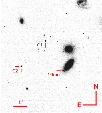
Figure 1. R-band image of SN 2019ein and the comparison stars taken with the Kanata telescope/HOWPol on MJD 58615.7 (2019 May 12).
Download figure:
Standard image High-resolution imageTable 1. Magnitudes of the Comparison Stars
| ID | U | B | V | R | I |
|---|---|---|---|---|---|
| (mag) | (mag) | (mag) | (mag) | (mag) | |
| C1 | 14.780 ± 0.099 | 14.621 ± 0.013 | 14.243 ± 0.012 | 14.011 ± 0.017 | 13.619 ± 0.023 |
| C2 | 15.583 ± 0.116 | 15.037 ± 0.015 | 14.478 ± 0.014 | 14.120 ± 0.019 | 13.638 ± 0.023 |
Download table as: ASCIITypeset image
Table 2. Log of Optical Observations of SN 2019ein
| Date | MJD | Phasea | U | B |

|
V | R | I | Telescope |
|---|---|---|---|---|---|---|---|---|---|
| (day) | (mag) | (mag) | (mag) | (mag) | (mag) | (mag) | (Instrument) | ||
| 2019 May 1 | 58604.8 | −13.4 | ⋯ | 18.255 ± 0.044 | ⋯ | 18.010 ± 0.077 | 17.619 ± 0.140 | 17.869 ± 0.023 | Kanata (HOWPol) |
| 2019 May 2 | 58605.5 | −12.7 | ⋯ | ⋯ | ⋯ | 17.211 ± 0.044 | 17.059 ± 0.103 | 17.318 ± 0.100 | Kanata (HOWPol) |
| 2019 May 3 | 58606.8 | −11.5 | ⋯ | 16.549 ± 0.019 | ⋯ | 16.473 ± 0.013 | 16.294 ± 0.018 | 16.284 ± 0.024 | Kanata (HOWPol) |
| 2019 May 4 | 58607.6 | −10.7 | ⋯ | ⋯ | ⋯ | 16.140 ± 0.012 | ⋯ | 15.852 ± 0.023 | Kanata (HOWPol) |
| 2019 May 5 | 58608.5 | −9.8 | ⋯ | ⋯ | 15.454 ± 0.066 | ⋯ | ⋯ | ⋯ | (MITSuME/AO) |
| 2019 May 6 | 58609.7 | −8.6 | ⋯ | 15.231 ± 0.018 | ⋯ | 15.260 ± 0.014 | 15.090 ± 0.017 | 15.022 ± 0.023 | Kanata (HOWPol) |
| 2019 May 7 | 58610.5 | −7.8 | ⋯ | ⋯ | 14.845 ± 0.049 | ⋯ | ⋯ | ⋯ | (MITSuME/AO) |
| 2019 May 7 | 58610.7 | −7.6 | ⋯ | 14.924 ± 0.014 | ⋯ | 14.967 ± 0.012 | 14.823 ± 0.018 | 14.775 ± 0.023 | Kanata (HOWPol) |
| 2019 May 8 | 58611.5 | −6.8 | ⋯ | ⋯ | 14.737 ± 0.031 | ⋯ | ⋯ | ⋯ | (MITSuME/AO) |
| 2019 May 8 | 58611.5 | −6.7 | 14.301 ± 0.207 | 14.635 ± 0.014 | ⋯ | 14.569 ± 0.191 | 14.657 ± 0.018 | 14.524 ± 0.028 | Pirika (MSI) |
| 2019 May 9 | 58612.5 | −5.8 | ⋯ | ⋯ | 14.625 ± 0.003 | ⋯ | ⋯ | ⋯ | (MITSuME/AO) |
| 2019 May 9 | 58612.6 | −5.6 | ⋯ | 14.446 ± 0.014 | ⋯ | 14.506 ± 0.013 | 14.418 ± 0.017 | 14.399 ± 0.025 | Kanata (HOWPol) |
| 2019 May 11 | 58614.5 | −3.7 | 14.036 ± 0.408 | 14.146 ± 0.015 | ⋯ | 14.175 ± 0.016 | 14.223 ± 0.017 | 14.185 ± 0.024 | Pirika (MSI) |
| 2019 May 11 | 58614.5 | −3.7 | ⋯ | ⋯ | 14.287 ± 0.023 | ⋯ | ⋯ | 14.106 ± 0.039 | (MITSuME/IAO) |
| 2019 May 11 | 58614.7 | −3.6 | ⋯ | 14.178 ± 0.014 | ⋯ | 14.205 ± 0.015 | 14.218 ± 0.019 | 14.218 ± 0.026 | Kanata (HOWPol) |
| 2019 May 12 | 58615.6 | −2.6 | 13.703 ± 0.107 | ⋯ | ⋯ | 14.072 ± 0.013 | 14.116 ± 0.018 | 14.084 ± 0.024 | Pirika (MSI) |
| 2019 May 12 | 58615.7 | −2.5 | ⋯ | 14.104 ± 0.013 | ⋯ | 14.104 ± 0.015 | 14.160 ± 0.017 | 14.186 ± 0.025 | Kanata (HOWPol) |
| 2019 May 13 | 58616.5 | −1.7 | ⋯ | 14.005 ± 0.014 | ⋯ | 14.017 ± 0.013 | 14.098 ± 0.017 | 14.134 ± 0.024 | Pirika (MSI) |
| 2019 May 14 | 58617.6 | −0.6 | 13.600 ± 0.100 | 13.972 ± 0.013 | ⋯ | 13.952 ± 0.013 | 14.061 ± 0.017 | 14.151 ± 0.029 | Pirika (MSI) |
| 2019 May 14 | 58617.6 | −0.6 | ⋯ | ⋯ | 13.986 ± 0.045 | ⋯ | ⋯ | ⋯ | (MITSuME/IAO) |
| 2019 May 15 | 58618.6 | 0.4 | 13.687 ± 0.099 | 13.977 ± 0.013 | ⋯ | 13.942 ± 0.013 | 14.050 ± 0.017 | 14.179 ± 0.023 | Pirika (MSI) |
| 2019 May 15 | 58618.7 | 0.4 | ⋯ | 14.013 ± 0.013 | ⋯ | 13.939 ± 0.014 | 14.072 ± 0.019 | 14.238 ± 0.024 | Kanata (HOWPol) |
| 2019 May 16 | 58619.5 | 1.2 | ⋯ | ⋯ | 14.122 ± 0.015 | ⋯ | ⋯ | ⋯ | (MITSuME/AO) |
| 2019 May 16 | 58619.6 | 1.4 | ⋯ | 14.058 ± 0.020 | ⋯ | 14.152 ± 0.113 | ⋯ | 14.279 ± 0.060 | Pirika (MSI) |
| 2019 May 17 | 58620.6 | 2.4 | ⋯ | 14.051 ± 0.014 | ⋯ | 14.118 ± 0.140 | ⋯ | 14.289 ± 0.023 | Pirika (MSI) |
| 2019 May 18 | 58621.6 | 3.4 | 13.769 ± 0.099 | 14.146 ± 0.013 | ⋯ | ⋯ | 14.080 ± 0.017 | 14.284 ± 0.024 | Pirika (MSI) |
| 2019 May 19 | 58622.5 | 4.3 | ⋯ | ⋯ | 14.140 ± 0.018 | ⋯ | ⋯ | ⋯ | (MITSuME/AO) |
| 2019 May 19 | 58622.6 | 4.4 | 13.915 ± 0.103 | 14.110 ± 0.014 | ⋯ | 14.016 ± 0.114 | 14.091 ± 0.017 | 14.288 ± 0.025 | Pirika (MSI) |
| 2019 May 21 | 58624.6 | 6.4 | ⋯ | ⋯ | 14.187 ± 0.012 | ⋯ | ⋯ | 14.259 ± 0.028 | (MITSuME/IAO) |
| 2019 May 23 | 58626.5 | 8.2 | ⋯ | ⋯ | 14.349 ± 0.027 | ⋯ | ⋯ | ⋯ | (MITSuME/AO) |
| 2019 May 23 | 58626.6 | 8.4 | ⋯ | 14.516 ± 0.017 | ⋯ | 14.126 ± 0.012 | 14.446 ± 0.017 | 14.689 ± 0.024 | Kanata (HOWPol) |
| 2019 May 24 | 58627.5 | 9.3 | ⋯ | ⋯ | 14.413 ± 0.031 | ⋯ | ⋯ | ⋯ | (MITSuME/AO) |
| 2019 May 25 | 58628.5 | 10.2 | ⋯ | 14.731 ± 0.013 | ⋯ | 14.276 ± 0.012 | 14.599 ± 0.020 | 14.822 ± 0.025 | Kanata (HOWPol) |
| 2019 May 25 | 58628.6 | 10.3 | ⋯ | ⋯ | 14.427 ± 0.025 | ⋯ | ⋯ | 14.613 ± 0.032 | (MITSuME/IAO) |
| 2019 May 26 | 58629.5 | 11.2 | ⋯ | ⋯ | 14.585 ± 0.035 | ⋯ | ⋯ | ⋯ | (MITSuME/AO) |
| 2019 May 26 | 58629.6 | 11.4 | ⋯ | 14.817 ± 0.013 | ⋯ | 14.372 ± 0.013 | 14.682 ± 0.019 | 14.871 ± 0.024 | Kanata (HOWPol) |
| 2019 May 29 | 58632.6 | 14.4 | ⋯ | 15.274 ± 0.014 | ⋯ | 14.586 ± 0.012 | 14.742 ± 0.019 | 14.808 ± 0.023 | Kanata (HOWPol) |
| 2019 Jun 3 | 58637.6 | 19.3 | ⋯ | 15.935 ± 0.018 | ⋯ | 14.842 ± 0.012 | 14.747 ± 0.018 | 14.612 ± 0.025 | Kanata (HOWPol) |
| 2019 Jun 8 | 58642.6 | 24.4 | ⋯ | 16.515 ± 0.013 | ⋯ | 15.181 ± 0.014 | 15.009 ± 0.023 | 14.625 ± 0.026 | Kanata (HOWPol) |
| 2019 Jun 12 | 58646.6 | 28.3 | ⋯ | 16.879 ± 0.020 | ⋯ | 15.526 ± 0.015 | 15.386 ± 0.020 | 14.994 ± 0.028 | Kanata (HOWPol) |
| 2019 Jun 15 | 58649.6 | 31.4 | ⋯ | ⋯ | 16.598 ± 0.019 | ⋯ | ⋯ | 15.046 ± 0.032 | (MITSuME/IAO) |
| 2019 Jun 17 | 58651.6 | 33.4 | ⋯ | ⋯ | ⋯ | 15.775 ± 0.013 | 15.722 ± 0.018 | 15.364 ± 0.023 | Kanata (HOWPol) |
| 2019 Jun 18 | 58652.5 | 34.3 | ⋯ | ⋯ | ⋯ | ⋯ | ⋯ | ⋯ | (MITSuME/AO) |
| 2019 Jun 19 | 58653.5 | 35.3 | ⋯ | 17.182 ± 0.021 | ⋯ | 15.868 ± 0.020 | 15.841 ± 0.020 | 15.493 ± 0.026 | Kanata (HOWPol) |
| 2019 Jun 23 | 58657.5 | 39.3 | ⋯ | 17.250 ± 0.017 | ⋯ | 15.978 ± 0.013 | 15.978 ± 0.020 | 15.697 ± 0.026 | Kanata (HOWPol) |
| 2019 Jun 25 | 58659.6 | 41.4 | ⋯ | 17.239 ± 0.021 | ⋯ | 16.029 ± 0.014 | 16.058 ± 0.018 | 15.791 ± 0.026 | Kanata (HOWPol) |
| 2019 Jul 2 | 58666.5 | 48.3 | ⋯ | 17.327 ± 0.110 | ⋯ | 16.230 ± 0.015 | 16.329 ± 0.030 | 16.118 ± 0.035 | Kanata (HOWPol) |
| 2019 Jul 4 | 58668.5 | 50.3 | ⋯ | 17.327 ± 0.021 | ⋯ | 16.282 ± 0.014 | 16.392 ± 0.018 | 16.242 ± 0.024 | Kanata (HOWPol) |
Note.
aRelative to the epoch of B-band maximum (MJD 58618.24).A machine-readable version of the table is available.
We also performed JHKs-band imaging observations with the Hiroshima Optical and Near-InfraRed camera (HONIR; Akitaya et al. 2014) attached to the 1.5 m Kanata telescope, and with the Nishi-harima Infrared Camera (NIC) installed at the Cassegrain focus of the 2.0 m Nayuta telescope at the NishiHarima Astronomical Observatory. We adopted the sky background subtraction using a template sky image obtained by the dithering observation. We performed the PSF-fitting photometry in the same way as used for the reduction of the optical data and calibrated the magnitudes using the comparison stars in the 2MASS catalog (Persson et al. 1998). All NIR photometric results are listed in Table 3.
Table 3. Log of NIR Observations of SN 2019ein
| Date | MJD | Phasea | J | H | Ks | Telescope |
|---|---|---|---|---|---|---|
| (day) | (mag) | (mag) | (mag) | (Instrument) | ||
| 2019 May 3 | 58606.7 | −11.5 | 16.315 ± 0.030 | 16.085 ± 0.120 | ⋯ | Kanata (HONIR) |
| 2019 May 5 | 58608.7 | −9.5 | ⋯ | 15.741 ± 0.031 | ⋯ | Kanata (HONIR) |
| 2019 May 6 | 58609.7 | −8.5 | 14.955 ± 0.033 | 14.821 ± 0.079 | 14.984 ± 0.067 | Kanata (HONIR) |
| 2019 May 7 | 58610.7 | −7.5 | 14.792 ± 0.032 | 14.801 ± 0.050 | 15.108 ± 0.042 | Kanata (HONIR) |
| 2019 May 9 | 58612.7 | −5.5 | 14.597 ± 0.121 | 14.877 ± 0.223 | 14.578 ± 0.131 | Kanata (HONIR) |
| 2019 May 10 | 58613.7 | −4.5 | 14.610 ± 0.033 | 14.687 ± 0.074 | 14.598 ± 0.166 | Kanata (HONIR) |
| 2019 May 12 | 58615.7 | −2.5 | 14.515 ± 0.050 | ⋯ | 14.476 ± 0.078 | Kanata (HONIR) |
| 2019 May 14 | 58617.5 | −0.7 | 14.640 ± 0.124 | 14.803 ± 0.083 | 14.490 ± 0.139 | Nayuta (NIC) |
| 2019 May 14 | 58617.6 | −0.6 | 14.747 ± 0.033 | 14.823 ± 0.223 | 14.586 ± 0.069 | Kanata (HONIR) |
| 2019 May 15 | 58618.6 | 0.4 | 14.510 ± 0.019 | 14.808 ± 0.109 | ⋯ | Kanata (HONIR) |
| 2019 May 15 | 58618.7 | 0.5 | 14.457 ± 0.070 | 14.846 ± 0.097 | 14.503 ± 0.195 | Nayuta (NIC) |
| 2019 May 16 | 58619.6 | 1.4 | 14.549 ± 0.040 | 14.770 ± 0.140 | ⋯ | Kanata (HONIR) |
| 2019 May 16 | 58619.7 | 1.5 | 14.871 ± 0.088 | 14.889 ± 0.116 | 14.560 ± 0.189 | Nayuta (NIC) |
| 2019 May 21 | 58624.5 | 6.3 | ⋯ | 15.047 ± 0.117 | 14.797 ± 0.209 | Nayuta (NIC) |
| 2019 May 21 | 58624.6 | 6.4 | 15.186 ± 0.025 | 14.976 ± 0.051 | 14.615 ± 0.027 | Kanata (HONIR) |
| 2019 May 22 | 58625.6 | 7.4 | 15.484 ± 0.035 | 15.370 ± 0.033 | 14.809 ± 0.045 | Kanata (HONIR) |
| 2019 May 24 | 58627.7 | 9.5 | ⋯ | ⋯ | 14.896 ± 0.221 | Nayuta (NIC) |
| 2019 May 28 | 58631.7 | 13.5 | ⋯ | 14.938 ± 0.039 | ⋯ | Kanata (HONIR) |
| 2019 May 29 | 58632.5 | 14.3 | ⋯ | 15.051 ± 0.115 | 14.944 ± 0.132 | Nayuta (NIC) |
| 2019 May 31 | 58634.6 | 16.4 | ⋯ | 14.954 ± 0.031 | ⋯ | Kanata (HONIR) |
| 2019 Jun 3 | 58637.5 | 19.3 | 15.694 ± 0.156 | 14.795 ± 0.055 | ⋯ | Nayuta (NIC) |
| 2019 Jun 3 | 58637.6 | 19.4 | 16.026 ± 0.030 | 15.076 ± 0.495 | ⋯ | Kanata (HONIR) |
| 2019 Jun 11 | 58645.6 | 27.4 | 15.491 ± 0.037 | ⋯ | ⋯ | Kanata (HONIR) |
| 2019 Jun 13 | 58647.6 | 29.4 | 15.864 ± 0.056 | ⋯ | ⋯ | Kanata (HONIR) |
| 2019 Jun 17 | 58651.6 | 33.4 | ⋯ | ⋯ | ⋯ | Kanata (HONIR) |
| 2019 Jun 24 | 58658.6 | 40.4 | ⋯ | ⋯ | ⋯ | Kanata (HONIR) |
Note.
aRelative to the epoch of B-band maximum (MJD 58618.24).A machine-readable version of the table is available.
Download table as: DataTypeset image
Additionally, we downloaded the imaging data obtained by the Swift Ultraviolet/Optical Telescope (UVOT) from the Swift Data Archive.19 We performed the PSF-fitting photometry using IRAF for these data. We calibrated the magnitudes using the comparison stars in the UBV bands. For the uvw1 and uvw2 bands, we adopted the absolute photometry using the zero points reported by Breeveld et al. (2011). All Swift/UVOT photometric results are listed in Table 4.
Table 4. Log of Swift/UVOT Observations of SN 2019ein
| Date | MJD | Phasea | V | B | U | uvw1 | uvw2 |
|---|---|---|---|---|---|---|---|
| (day) | (mag) | (mag) | (mag) | (mag) | (mag) | ||
| 2019 May 2 | 58605.4 | −12.8 | 17.625 ± 0.128 | 17.594 ± 0.069 | 17.833 ± 0.077 | 20.781 ± 0.448 | 20.667 ± 0.437 |
| 2019 May 3 | 58606.4 | −11.8 | 16.570 ± 0.204 | 16.607 ± 0.040 | 16.731 ± 0.063 | 18.591 ± 0.161 | 19.802 ± 0.214 |
| 2019 May 4 | 58607.8 | −10.4 | 15.793 ± 0.045 | 15.895 ± 0.037 | 15.788 ± 0.051 | 17.872 ± 0.079 | 18.888 ± 0.109 |
| 2019 May 5 | 58608.8 | −9.4 | 15.490 ± 0.045 | 15.476 ± 0.034 | 15.317 ± 0.037 | 17.035 ± 0.077 | 18.314 ± 0.066 |
| 2019 May 6 | 58609.7 | −8.5 | 15.114 ± 0.040 | 15.092 ± 0.035 | 14.956 ± 0.040 | 16.681 ± 0.061 | 18.208 ± 0.074 |
| 2019 May 9 | 58612.6 | −5.6 | ⋯ | ⋯ | ⋯ | 15.748 ± 0.038 | 17.026 ± 0.054 |
| 2019 May 12 | 58615.5 | −2.7 | 14.107 ± 0.036 | 14.006 ± 0.026 | 13.912 ± 0.046 | 15.755 ± 0.042 | 16.747 ± 0.048 |
| 2019 May 14 | 58617.2 | −1.0 | ⋯ | ⋯ | ⋯ | 16.937 ± 0.040 | 16.937 ± 0.040 |
| 2019 May 14 | 58617.2 | −1.0 | ⋯ | ⋯ | ⋯ | 16.769 ± 0.063 | 16.769 ± 0.063 |
| 2019 May 16 | 58619.1 | 0.9 | ⋯ | ⋯ | ⋯ | 15.637 ± 0.035 | 16.787 ± 0.055 |
| 2019 May 17 | 58620.1 | 1.9 | 13.899 ± 0.039 | 13.913 ± 0.038 | ⋯ | 15.758 ± 0.052 | 16.755 ± 0.039 |
| 2019 May 26 | 58629.2 | 11.0 | ⋯ | ⋯ | ⋯ | ⋯ | 18.157 ± 0.034 |
| 2019 May 26 | 58629.3 | 11.1 | ⋯ | ⋯ | ⋯ | ⋯ | 17.769 ± 0.075 |
| 2019 May 27 | 58630.2 | 12.0 | ⋯ | ⋯ | ⋯ | ⋯ | 18.078 ± 0.050 |
Note.
aRelative to the epoch of B-band maximum (MJD 58618.24).A machine-readable version of the table is available.
Download table as: DataTypeset image
2.2. Spectroscopy
We obtained optical spectra of SN 2019ein using HOWPol. The wavelength coverage is 4500–9200 Å, and the wavelength resolution is R = λ/Δλ ≃ 400 at 6000 Å. For wavelength calibration, we used sky emission lines. To remove cosmic-ray events, we used the L. A. Cosmic pipeline (van Dokkum 2001; van Dokkum et al. 2012). The flux of SN 2019ein was calibrated using the data of spectrophotometric standard stars taken on the same nights.
In addition, we obtained optical spectroscopic data using the Kyoto Okayama Optical Low-dispersion Spectrograph with an integral field unit (KOOLS-IFU; Yoshida 2005; Matsubayashi et al. 2019) installed on the 3.8 m Seimei telescope through the optical fibers. The Seimei telescope of Kyoto University is a newly established telescope at the Okayama Observatory (Kurita et al. 2010). The data were taken under the programs 19A-1-CN07, 19A-1-CN09, 19A-1-CT01, 19A-K-0003, 19A-K-0004, and 19A-K-0010. KOOLS-IFU is equipped with four grisms, among which we used the VPH-blue. The wavelength coverage is 4000–8900 Å, and the wavelength resolution is R = λ/Δλ ∼ 500. The data reduction was performed using the Hydra package in IRAF (Barden et al. 1994; Barden & Armandroff 1995) and a reduction software specifically developed for KOOLS-IFU data. For the wavelength calibration, we used arc lamp (Hg and Ne) data. A lot of the spectroscopic observations are listed in Table 5.
Table 5. Log of the Spectroscopic Observations of SN 2019ein
| Date | MJD | Phasea | Coverage | Resolution | Telescope |
|---|---|---|---|---|---|
| (day) | (Å) | (Instrument) | |||
| 2019 May 3 | 58606.7 | −11.5 | 4000–8900 | 500 | Seimei (KOOLS) |
| 2019 May 5 | 58608.8 | −9.5 | 4500–9200 | 400 | Kanata (HOWPol) |
| 2019 May 6 | 58609.7 | −8.5 | 4000–8900 | 500 | Seimei (KOOLS) |
| 2019 May 9 | 58612.6 | −5.6 | 4000–8900 | 500 | Seimei (KOOLS) |
| 2019 May 11 | 58614.7 | −3.6 | 4500–9200 | 400 | Kanata (HOWPol) |
| 2019 May 12 | 58615.7 | −2.6 | 4000–8900 | 500 | Seimei (KOOLS) |
| 2019 May 14 | 58617.6 | −0.6 | 4000–8900 | 500 | Seimei (KOOLS) |
| 2019 May 21 | 58624.6 | 6.4 | 4500–9200 | 400 | Kanata (HOWPol) |
| 2019 May 29 | 58632.5 | 14.2 | 4000–8900 | 500 | Seimei (KOOLS) |
| 2019 Jun 11 | 58645.6 | 27.4 | 4500–9200 | 400 | Kanata (HOWPol) |
| 2019 Jun 12 | 58646.6 | 28.4 | 4500–9200 | 400 | Kanata (HOWPol) |
| 2019 Jun 19 | 58653.6 | 35.3 | 4500–9200 | 400 | Kanata (HOWPol) |
| 2019 Jun 25 | 58659.6 | 41.4 | 4500–9200 | 400 | Kanata (HOWPol) |
Note.
aRelative to the epoch of B-band maximum (MJD 58618.24).A machine-readable version of the table is available.
Download table as: DataTypeset image
3. Results
3.1. Light Curves
Based on the spectral similarity to HV SN 2002bo in the classification spectrum (Burke et al. 2019) and further analyses of the spectral properties, which also suggest the HV SN Ia classification for SN 2019ein (see Sections 3.3 and 3.4 for details), we specifically focus on the comparison of its light curves to those of HV SNe Ia.
Figure 2 shows the multiband light curves of SN 2019ein. We estimate the epoch of the B-band maximum as MJD 58618.24 ± 0.07 (2019 May 15.2) by performing a polynomial fitting to the data points around maximum light. In this paper, we refer to the B-band maximum date as day zero. We derived the decline rate in the B band as Δm15(B) = 1.36 ± 0.02 mag. As compared to some well-studied HV SNe Ia, SN 2019ein shows a faster decline than SNe 2002bo (1.13 ± 0.05 mag; Benetti et al. 2004), 2002dj (1.08 ± 0.05 mag; Pignata et al. 2008), and 2004dt (1.21 ± 0.05 mag; Altavilla et al. 2007). The decline rate is similar to that of HV SN 2002er (1.33 ± 0.04 mag; Pignata et al. 2004). The B-band maximum magnitude is 13.99 ± 0.03 mag. The maximum date, the peak magnitude, and the decline rate in the BVRI bands are listed in Table 6.
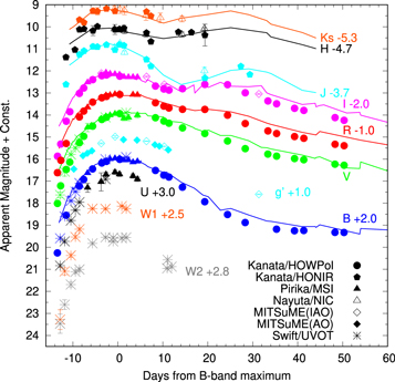
Figure 2. Multiband light curves of SN 2019ein. The different symbols denote data that were obtained using different instruments (see the figure legends). The light curve of each band is shifted vertically as indicated in the figure. We adopted MJD 58618.24 ± 0.07 as day zero. For comparison, we show the light curves of SN 2002bo with solid lines (Benetti et al. 2004; Krisciunas et al. 2004).
Download figure:
Standard image High-resolution imageTable 6. Parameters of the BVRI-band Light Curves for SN 2019ein
| Band | Maximum Date | Maximum Magnitude | Δm15 | Δta |
|---|---|---|---|---|
| (MJD) | (mag) | (mag) | (days) | |
| I | 58616.75 (0.10) | 14.15 (0.02) | 0.76 (0.06) | −1.49 |
| R | 58619.18 (0.08) | 14.08 (0.02) | 0.45 (0.16) | +0.94 |
| V | 58619.76 (0.08) | 13.92 (0.02) | 0.76 (0.01) | +1.52 |
| B | 58618.24 (0.07) | 13.99 (0.03) | 1.36 (0.02) | ⋯ |
Note.
aThe time difference from the B-band maximum.Download table as: ASCIITypeset image
Figure 3 shows the B-band light curves of SN 2019ein, well-studied HV SNe, and NV SN 2011fe. This highlights that the observation for SN 2019ein started at the most infant phase among HV SNe. Although the data in the rising part of HV SNe are limited, it is clear that SN 2019ein shows a fast rise and decline. The decline of SN 2019ein is as fast as that of SN 2002er.
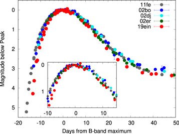
Figure 3. B-band light curve of SN 2019ein. For comparison, we plot that of SNe 2002bo (Benetti et al. 2004; Krisciunas et al. 2004), 2002dj (Pignata et al. 2008), 2002er (Pignata et al. 2004), and 2011fe (Zhang et al. 2016). The inset panel shows that the light curves expanded around maximum light.
Download figure:
Standard image High-resolution imageThe decline rate is consistent with other observational properties. The time interval between the first peak and the second peak in the I band shows a correlation with Δm15(B) (Elias-Rosa et al. 2008). The relation predicts the time interval to be 24.33 ± 0.26 days. From the light curve, the interval is derived to be 24.76 ± 2.82 days, being consistent with that expected from Δm15(B). The line-depth ratio of Si ii λ5972 to Si ii λ6355 is an indicator of the absolute magnitude (Nugent et al. 1995) or Δm15(B) (Blondin et al. 2012). A similar relation also exists for the ratio of the pseudo-equivalent widths (pEWs). These ratios measured for SN 2019ein are also consistent with Δm15(B) (see Section 3.3).
3.2. Absolute Magnitude
To estimate the extinction within the host galaxy and the absolute magnitude of SN 2019ein, we apply a light-curve fitter (SNooPy; Burns et al. 2011) to the light curves of SN 2019ein. We then obtain  (statistical) ± 0.06 (systematic) mag with RV = 1.5 (see below). As a cross-check, we use phenomenological relations to estimate the host extinction, based on the B − V color. The B − V color at the maximum light of SN 2019ein is 0.05 ± 0.02 mag after correcting for the MW extinction with
 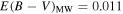 mag and RV = 3.1 (Schlafly & Finkbeiner 2011). We may use the relation between the intrinsic B − V color and the decline rate; we obtain
  mag using the relation by Phillips et al. (1999), or
  mag using that given by Reindl et al. (2005). We may also use the relation between the line velocity of Si ii λ6355 and the intrinsic B − V color at maximum light; we obtain
  mag using the relation by Foley et al. (2011), or 0.14 ± 0.08 mag using that presented by Blondin et al. (2012). The values estimated by the different methods largely agree with each other, and we adopt
  mag obtained by SNooPy throughout the paper. The estimated extinction is not large and will not affect the main conclusions in the present work.
In Table 7, we show the B-band peak absolute magnitudes of SN 2019ein that are estimated using the luminosity–width relations given in the previous papers. The derived values for the absolute magnitude agree with each other within the uncertainty. The average value is −19.14 ± 0.10 mag. From the estimated peak absolute magnitude,  mag and RV = 1.55 ± 0.06 (as is frequently adopted for HV SNe; Wang et al. 2009), we obtain the distance to SN 2019ein (NGC 5353) as μ = 32.95 ± 0.12 mag. The value is larger than that from the NASA/IPAC Extragalactic Database (NED)20
(μ = 32.20 ± 0.54 mag). However, the distance measurements for NGC 5353 found in NED are highly uncertain,21
and we think that the distance obtained here assuming that SN 2019ein follows the SN Ia luminosity–width/color relation is indeed more robust than previous estimates; SN 2019ein shows various properties in the light curves and the spectra that fit into the correlations found for a sample of SNe Ia, and therefore, it is rational to assume that the SN also follows the standardized candle relation. In what follows, we use
mag and RV = 1.55 ± 0.06 (as is frequently adopted for HV SNe; Wang et al. 2009), we obtain the distance to SN 2019ein (NGC 5353) as μ = 32.95 ± 0.12 mag. The value is larger than that from the NASA/IPAC Extragalactic Database (NED)20
(μ = 32.20 ± 0.54 mag). However, the distance measurements for NGC 5353 found in NED are highly uncertain,21
and we think that the distance obtained here assuming that SN 2019ein follows the SN Ia luminosity–width/color relation is indeed more robust than previous estimates; SN 2019ein shows various properties in the light curves and the spectra that fit into the correlations found for a sample of SNe Ia, and therefore, it is rational to assume that the SN also follows the standardized candle relation. In what follows, we use  mag and μ = 32.95 ± 0.12 mag unless otherwise mentioned.
3.3. Spectral Properties
Figure 4 shows the optical spectra of SN 2019ein from −11.5 days through 41.4 days. The spectra are characterized by absorption lines of Si ii, S ii, Fe ii, and Fe iii and the Ca ii IR triplet. The spectra of SN 2019ein show a striking similarity to those of HV SN 2002bo.
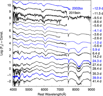
Figure 4. Spectral evolution of SN 2019ein (black lines). The epoch for each spectrum is indicated on the right outside the panel. For comparison, we plot the spectra of SNe 2002bo (blue lines; Benetti et al. 2004; Blondin et al. 2012).(The data used to create this figure are available.)
Download figure:
Standard image High-resolution imageBranch et al. (2006) suggested that SNe Ia are classified into four subgroups using the EWs of Si ii λ5792 and Si ii λ6355. The pEWs of Si ii λ5792 and Si ii λ6355 measured for SN 2019ein at −0.6 days are 133.24 ± 4.16 Å and 25.65 ± 2.98 Å, respectively. In Figure 5, we show the Branch et al. (2006) diagram. In this classification scheme, SN 2019ein is classified as the “broad-line (BL)” subgroup, the distribution of which overlaps with HV SNe (Wang et al. 2009). The pEW ratio of Si ii λ5972 and Si ii λ6355, and the depth ratio of these lines are 0.23 ± 0.03 and 0.19 ± 0.02, respectively. From Figure 14 of Blondin et al. (2012), these ratios are consistent with Δm15(B). SN 2019ein is thus classified as an HV (and BL) SN Ia from its maximum-light spectrum, irrespective of the nature of the spectra in the pre-maximum phase.
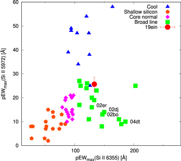
Figure 5. Pseudo-equivalent widths of Si ii λ6355 and Si ii λ5792. The comparison samples are from Silverman et al. (2012a). Note that the “Broad Line” and “Core Normal” classes correspond to the HV and NV classes.
Download figure:
Standard image High-resolution imageWe therefore apply a single-Gaussian fit to the absorption-line profiles to study the evolution of the line velocities, in the same manner applied to HV SNe in previous studies.22 For each spectrum, the fit is performed several times with the continuum determination varied, using the splot task in IRAF. We determined the uncertainty from the rms of the standard deviation in the fits and the wavelength resolution. In Figure 6, we compare the evolution of the line velocity of Si ii λ6355 to that of other HV SNe, and to that of SN 2012fr, which showed strong HVFs. SN 2019ein is among SNe that show the fastest line velocities in the early phase. The line velocity of SN 2019ein is ∼20,000 km s−1 at −12 days, and it is as fast as that of SN 2006X and the HVF component seen in SN 2012fr. SN 2019ein shows a rapid evolution in velocity toward the B-band maximum. The velocity of SN 2019ein decreases to ∼14,000 km s−1 at −0.6 days. Around maximum light, it becomes similar to that of SN 2002bo, despite the initially larger velocity. After maximum light, the velocity evolution of SN 2019ein flattens at ∼12,000 km s−1.
Figure 6. Evolution of the line velocity of Si ii λ6355 in SN 2019ein. For comparison, we plot those for SNe 2002bo (Benetti et al. 2004; Blondin et al. 2012; Silverman et al. 2012a), 2002dj (Pignata et al. 2008), 2002er (Kotak et al. 2005; Blondin et al. 2012; Silverman et al. 2012a), 2004dt (Altavilla et al. 2007), 2006X (Yamanaka et al. 2009), and 2012fr (Childress et al. 2013; the open and filled circles denote the velocity of the high-velocity feature component and the photospheric component, respectively). The red solid line is a polynomial function that fits the data of SN 2019ein.
Download figure:
Standard image High-resolution imageFigure 7 shows an expanded view of the Si ii λ6355 feature at several phases. Initially, at ∼−12 days, the feature resembles that of SN 2012fr, which is dominated by the HVF component. However, subsequent evolution is different; SN 2012fr developed two distinct features interpreted as the detached HVF and the photospheric components, where the latter show slow evolution in velocity (Childress et al. 2013). On the other hand, SN 2019ein does not develop clear multiple features, and a single component seems to continuously move toward lower velocity as time goes by (see Section 3.4 for further details). This property is consistent with the evolution of Si ii in HV SNe. In the first epoch, the velocities of Si ii seen in HV SNe 2002bo, 2002dj, and 2004dt are slower than that of SN 2019ein. However, the line width and strength are almost the same in these SNe Ia including SN 2019ein, again confirming the classification of SN 2019ein as an HV SN Ia. At −9 days, SN 2019ein rather resembles SNe 2002bo and 2002dj, and is clearly different from SN 2012fr. The photospheric component of SN 2012fr is now as noticeable as the HVF one, but such a behavior is never seen for SN 2019ein; while the spectrum of SN 2019ein at −9.5 days is noisy, it is still consistent with a single component. Toward maximum light, SN 2019ein becomes more and more similar to SNe 2002bo and 2002dj, and the difference between SNe 2019ein and 2012fr becomes more noticeable. Among the sample, SN 2004dt shows a broad and boxy Si ii line profile unlike the other comparison SNe Ia. We note that SN 2004dt is indeed suggested to be an outlier in the HV class (Maeda et al. 2010).
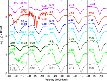
Figure 7. Evolution of the Si ii λ6355 line profile of SN 2019ein as shown in velocity space. For comparison, we show the spectra of SNe 2012fr (Childress et al. 2013), 2002bo (Benetti et al. 2004; Blondin et al. 2012), 2002er (Kotak et al. 2005), 2002dj (Pignata et al. 2008), 2004dt (Altavilla et al. 2007), and 2011fe (Pereira et al. 2013).
Download figure:
Standard image High-resolution imageWe estimate the velocity gradient of Si ii λ6355. In this paper, we obtain the velocity gradient using the method of Foley et al. (2011), in which the velocity gradient is estimated by fitting a liner function to the velocity evolution within a fixed time interval (−6 days ≤ t ≤ 10 days). Following this definition, we derive the velocity gradient of SN 2019ein as 235.3 ± 61.7 km s−1 day−1. By the same method, we also estimate the velocity gradient of other SNe Ia as follows: SNe 2002bo (215.1 ± 23.3 km s−1 day−1), 2004dt (243.5 ± 18.2 km s−1 day−1), 2006X (239.6 ± 18.4 km s−1 day−1), 2002er (119.7 ± 14.5 km s−1 day−1), and 2002dj (136.4 ± 15.1 km s−1 day−1). SN 2019ein shows a velocity gradient similar to SNe 2002bo, 2004dt, and 2006X, and larger than SNe 2002er and 2002dj.
The velocity gradient defined at maximum light has been suggested to be correlated to the Si velocity at maximum light (Foley 2012; Wang et al. 2013). SN 2019ein fits into this relation. However, the present study shows that it is not necessarily the case for the pre-maximum, sufficiently early phases. Despite a lower Si velocity at maximum light than SNe 2006X and 2004dt, the velocity of SN 2019ein evolves much faster in the pre-maximum phase than these SNe. Because of this evolution effect, the Si ii λ6355 velocity in the early phase of SN 2019ein is among the largest in the HV SN group, despite only a moderately large velocity at maximum light. This indicates that diversity exists within the HV SN group. While the speed of the spectral evolution around maximum light is highly dependent on the velocity observed there, it is more strongly correlated with Δm15(B) (or generally the speed of the evolution in the light curves) in the pre-maximum phase. We note that such a correlation between the spectral evolution and Δm15(B) is indeed well known for NV SNe (e.g., Benetti et al. 2005), but has not been clarified for HV SNe due to the limited sample.
3.4. High-velocity Features?
It has been suggested that most, if not all, SNe Ia show the so-called HVF detached from the photospheric component, if spectra are taken sufficiently early. For NV SNe, the HVF and photospheric components can be well separated in velocity space (e.g., see Figure 7 for SN 2012fr). This may not be the case for HV SNe where the line blending between two components, even if the HVF exists, can be significant. As such, one may ask if the high-velocity “photospheric” component in the earliest phases might be contaminated substantially by the possible HVF, which would overestimate the absorption velocity derived from a single-component fit. In this section, we further investigate the possibility of whether the HVFs could contaminate the early-phase spectra, and if this contamination would mimic the high-velocity “single component.” Note that this is indeed a general issue for HV SNe, not only for SN 2019ein. In Figure 8, we show the evolution of the pEW and velocity of Si ii λ6355. In the case of SN 2019ein, the pEW gradually decreases as time goes on. SNe 2002bo and 2002er show similar evolution. The behavior is very different from that found for SN 2012fr.
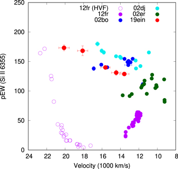
Figure 8. Evolution of pseudo-equivalent width vs. velocity of Si ii λ6355 for SN 2019ein. For comparison, we plot those of SNe 2002bo (Benetti et al. 2004; Blondin et al. 2012; Silverman et al. 2012a), 2002dj (Pignata et al. 2008), 2002er (Kotak et al. 2005; Silverman et al. 2012a), and 2012fr (Childress et al. 2013; the open and filled circles denote the velocity of the high-velocity-feature component and the photospheric component, respectively).
Download figure:
Standard image High-resolution imageTo further quantify the issue, we fit the profile of Si ii λ6355 with a combination of two Gaussian functions, for SNe 2012fr and 2019ein. The early-phase spectra of SN 2012fr show two obviously distinct components. It is seen that the FWHMs of the HVF and photospheric components both remain almost unchanged over time (Childress et al. 2013). At maximum light, the Si ii λ6355 line shows the photospheric component only. We thus measure the FWHM of the photospheric component at this phase and use the same FWHM for the other epochs. With the FWHM of the photospheric component fixed, we vary the remaining parameters (the velocities of both components, the FWHM of the HVF, and the relative depth) to fit each spectrum. Figure 9 shows that the spectra of SN 2012fr before maximum light are well fit by a combination of HVF and photospheric components. The results of the fits (e.g., the velocities of the two components) are consistent with those of Childress et al. (2013).
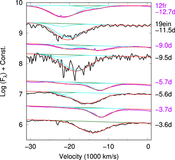
Figure 9. Two-component fit to the Si ii λ6355 line of SN 2019ein (black lines) and to that of SN 2012fr (Childress et al. 2013; purple lines) before maximum light. We plot the pseudo-continuum and two individual components as the dark green and cyan lines, respectively. The sums of these components are shown as the red lines.
Download figure:
Standard image High-resolution imageThe two-Gaussian fit to the spectra of SN 2019ein follows the same manner. First, we fit the FWHM of the photospheric component using the maximum-light spectrum. With this fixed, the velocity of the photospheric component can be well constrained for each spectrum, by fitting the line profile on the red side where the contribution by the possible HVF should be essentially zero. The residual on the blue side is then practically associated with the HVF, which allows the velocity and the FWHM of the possible HVF at each epoch to be constrained. Because the spectra of SN 2019ein are well fit by a single-Gaussian function, obviously the two-component fit works as well (Figure 9). However, the contribution by the HVF is negligibly small at all epochs. The velocity and the pEW of Si ii λ6355 (in the photospheric component) are little influenced by introducing the additional HVF contribution.
This result is consistent with a previous statistical study of the HVFs, given a small Δm15(B) for SN 2019ein; the HVFs are less frequently found, at a given epoch, for more rapidly declining SNe (Childress et al. 2013; Zhao et al. 2016). Detecting the HVFs for the (relatively) rapid decliner would require extremely rapid follow-up spectroscopy. Indeed, the first spectrum for SN 2019ein reported by the LCO Global SN project, taken within a day of the discovery23 (Burke et al. 2019), shows clear HVFs both for the Ca ii H&K and Ca ii NIR, the latter perhaps contaminating the HVF of O i λ7774. There is further a hint of the HVF of Si ii λ6355, which shows a faster velocity than Si ii λ5972. The characteristic velocity of these HVFs is ∼25,000–30,000 km s−1. The velocities seen in these clear HVFs are even much faster than the velocities of the photospheric component studied here, by ∼10,000 km s−1, and thus it is nearly impossible that it would substantially affect our analysis.
In summary, SN 2019ein belongs to the HV SN Ia group. The very high velocity found for SN 2019ein probably stems from the very early discovery and follow-up. SN 2019ein therefore serves as the best-studied example of an HV SN with a relatively large Δm15(B).
4. Discussion
4.1. Light Curves in the Rising Phase
We obtained multiband light curves of SN 2019ein from the early rising part presumably soon after the explosion. From these data, we try to constrain the explosion date and the rise time. We assume the homologously expanding “fireball model” (Arnett 1982; Riess et al. 1999; Nugent et al. 2011) to estimate the explosion date. In this model, the luminosity/flux (f) increases as f ∝ t2, where t is the time since the zero point. In this paper, we assume that the zero point in the time axis in this relation is the same for different bands (i.e., the explosion date), and adopt the same power-law index of 2 in all BVRI bands.
In Figure 10, we show that the early light curves are well fit by the fireball model. The rising part of SN 2019ein, in all the BVRI bands, can be explained by this simple fireball model. using the fitting, we estimate the explosion date as MJD 58602.87 ± 0.55. There is no significant deviation from the fireball model, at least after ∼2 days from the putative explosion date. No excess is found with respect to the fireball prediction. There is also no need to introduce a broken power law in the early phase.
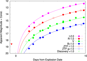
Figure 10. Optical light curves of SN 2019ein in the early phase. We also plot the discovery magnitude (the cross symbol; Tonry et al. 2019) and the data obtained by ZTF taken from the Transient Name Server. The red and blue open circles denote data in the r and g bands, respectively. The upside-down triangle indicates the upper-limit magnitude obtained by ZTF. The explosion date is estimated to be MJD 58602.87 ± 0.55 using a quadratic function (see Section 4.1).
Download figure:
Standard image High-resolution imageFrom the earliest portion of the rising light curve, we now discuss implications for the progenitor system. The ejecta of SNe Ia are expected to collide with a companion star and create additional heat and thermal energy. The thermal energy is then lost quickly, due to the adiabatic expansion (e.g., Kasen 2010), but a small fraction will be leaving the system as radiation. The expected strength and duration of this emission are larger for a more extended companion star. Therefore, through the nondetection of such an emission signal, one can place an upper limit on the radius of the companion star. We constrain the radius of the companion star of SN 2019ein by scaling the parameters found in the previous analysis conducted for SN 2011fe (Nugent et al. 2011). They estimated the luminosity of SN 2011fe in the early phase from g-band observation. At 1.9 days from the explosion, the luminosity of SN 2019ein is (2.7–3.6) × 1041 erg s−1. By scaling the result of Nugent et al. (2011) using the relation suggested by Kasen (2010), we obtain the upper limit of the companion’s radius as 4.3–7.6 R⊙. It thus excludes a red giant companion oriented along the line of sight. We, however, note that this does not rule out an evolutionary scenario where a giant companion star has already evolved to a WD (Justham 2011; Di Stefano & Kilic 2012; Hachisu et al. 2012).
The rise time, which is a measure of the time interval between the explosion and maximum light, may also provide some insights into the explosion property, and its correlation with other observational features has been investigated (e.g., Hayden et al. 2010; Ganeshalingam et al. 2011; Jiang et al. 2020). The rise time, defined as the B-band maximum date minus the estimated explosion date, is 15.37 ± 0.55 days for SN 2019ein. It is shorter than that of SN 2002bo (17.9 ± 0.5 days; Benetti et al. 2004) or SN 2002er (18.7 days; Pignata et al. 2004).
There is a tendency for SNe Ia that have smaller Δm15(B) (i.e., slower decline) to show a longer rise time (e.g., Perlmutter et al. 1998; Hayden et al. 2010; Ganeshalingam et al. 2011). The rise time derived here for SN 2019ein indeed fits the distribution of Δm15 versus the rise time for the HV SNe in Figure 6 of Ganeshalingam et al. (2011). SN 2002bo has a smaller Δm15(B) than SN 2019ein, and it is consistent with SN 2002bo having a longer rise time. Indeed, in this respect, SN 2002er, with a similar Δm15(B) to SN 2019ein but a longer rise time than SN 2002bo, does not recover the correlation between Δm15(B) and the rise time (Pignata et al. 2004).
This might indicate that Δm15(B) is not a single function that determines the rise time. For example, the velocity may have a role as a second parameter, given the diversity in velocities seen for HV SNe; it is faster for SN 2019ein than SN 2002er (Figure 6) despite similar Δm15(B). Indeed, HV SNe appear to have a faster rise time in the B band than NV SNe (Pignata et al. 2008; Zhang et al. 2010; Ganeshalingam et al. 2011) for given Δm15(B). In summary, we find that the evolution of HV SNe in the pre-maximum phase, both spectroscopically and photometrically, is controlled not only by Δm15(B) but also by the velocity (at maximum light). The evolution of the light curve and the velocity may provide an important constraint on the nature of the ejecta structure. Importantly, it does not form a one-parameter family.
4.2. Structure of the Outermost Layers
A spectral time series of SNe provides an opportunity to study the composition structure within the ejecta (Stehle et al. 2005; Mazzali et al. 2008; Tanaka et al. 2011; Sasdelli et al. 2014). Given that the photosphere generally recedes in velocity space as time goes on due to the density decrease, one can probe the property of the outer layer from the spectra taken earlier. The spectra presented here start with ∼−12 days and then ∼−10 days, which are comparable to the phase of the first spectrum taken for the well-studied HV SN Ia 2002bo. Indeed, given the rapidly evolving nature of SN 2019ein (Section 3.1) and the short rise time (Section 4.1), the estimated explosion date suggests that these spectra were obtained shortly after the explosion, ∼3.7 and ∼5.7 days after the explosion for these spectra. These are among the most infant spectra taken for SNe Ia, especially as an HV SN. We note that the first classification-report spectrum was already taken 0.82 days since the discovery, which is likely ∼2.4 days since the explosion (Section 3.4).
We use two of our spectra taken at the earliest phases to study the composition structure of the outermost layer of SN 2019ein, which may hint at the general property of HV SNe. We note that the possible decomposition of the absorption lines into photospheric and HVF components (Section 3.4) is merely an “interpretation,” and the analysis here is totally independent from such an issue. In doing this, we perform one-dimensional (spherically symmetric) spectral synthesis calculations using TARDIS24 (Kerzendorf & Sim 2014). To simplify the problem, we adopt a power-law density structure above 17,000 km s−1, with the normalization matched to the classical W7 model at this inner boundary. While there is a drop in the density in the W7 model beyond ∼20,000 km s−1, we keep the same density slope beyond this. We note that there is a diversity seen in this outermost density structure for different models, and our density structure is well within the model predictions (see, e.g., Figure 3 of Mazzali et al. 2014). Given the observed spectral lines showing high velocity in the earliest spectra of SN 2019ein, at least a moderate amount of material above 20,000 km s−1 is required.
Given the large degree of freedom even in the 1D model and the nonlinear nature of the problem to solve, there is no guarantee that the spectral synthesis model provides a unique solution. After testing various possibilities, we have decided to adopt the simplest approach, based on underlying nuclear-burning physics. In our model, we consider only two characteristic layers: an inner O–Ne–C burning layer and an outer unburnt C + O layer. In the O–Ne–C burning layer, the mass fractions are set as follows: 0.68 (O), 0.025 (Ne), 0.1 (Mg), 0.2 (Si), 0.025 (S), and 5e−4 (Ca). In the unburnt layer, we adopt the following: 0.5 (C), 0.475 (O), and 0.025 (Ne). The solar abundances are added for the heavier elements in both layers. Note that these compositions represent well those in the outermost layers found in the hydrodynamic and nucleosynthesis simulations, without introducing mixing between different layers. In the W7 model, these two layers are found at ∼13,000–15,000 km s−1 and >15,000 km s−1 for the O–Ne–C burning and unburnt regions, respectively. In the delayed detonation model CS15DD2 of Iwamoto et al. (1999), these are ∼18,000–30,000 km s−1 and >30,000 km s−1, respectively.
Figure 11 shows how this simple model can indeed reproduce the earliest-phase spectra of SN 2019ein reasonably well. Note that we do not aim to obtain a detailed fit, because we restrict ourselves to the simple model without fine-tuning. We assume that the explosion date is 1.6 days before the discovery, the distance modulus is 33.0 mag, and  mag and RV = 1.5. We determine the photospheric velocity to be 20,000 km s−1 and 17,000 km s−1 at −11.5 and −9.5 days (3.7 and 5.7 days since the assumed explosion date), respectively. The photospheric velocities found here are extremely high; these are ∼13,000–14,000 km s−1 and ∼12,000–13,000 km s−1 at similar phases (since the explosion) found for the best-studied NV SN Ia 2011fe (Mazzali et al. 2014), confirming that HV SNe show exceedingly higher velocity in the earlier phases. The velocities found here are even higher than those found for the prototypical HV SN 2002bo at similar epochs, as already indicated by the spectral comparison. This indicates a large diversity among the HV SN class and places SN 2019ein into the most extreme example in terms of the line velocity in the pre-maximum phase. This is likely related to the rapidly evolving nature of SN 2019ein in its light curves (Sections 3.1 and 4.1).
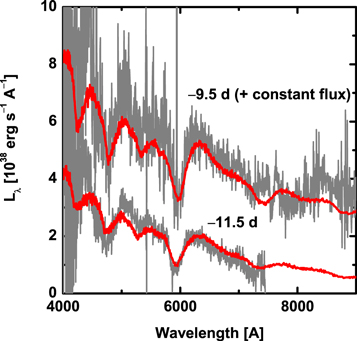
Figure 11. Comparison of the observed spectra at −11.5 and −9.5 days (gray lines) to the synthesized spectra (red lines) calculated with TARDIS. These observed spectra are corrected for the MW and the host galaxy extinction.
Download figure:
Standard image High-resolution imageFigure 12 shows how the velocity at the interface between the burnt and unburnt layers can be constrained. We note that the overall spectral appearance is not sensitive to this velocity, but the line profile is. As long as this velocity is larger than ∼30,000 km s−1, the Si ii profile does not change significantly. On the other hand, once the interface velocity is set below ∼30,000 km s−1, the line profile shifts to the lower velocity as this interface is moved toward a deeper region. From this exercise, we place the constraint that the burnt/unburnt interface is at >30,000 km s−1. Note that we do not require, indeed disfavor, the mixing of the inner, more advanced burning region (such as the Si burning) into the region above ∼17,000 km s−1 as we probe using these spectra.
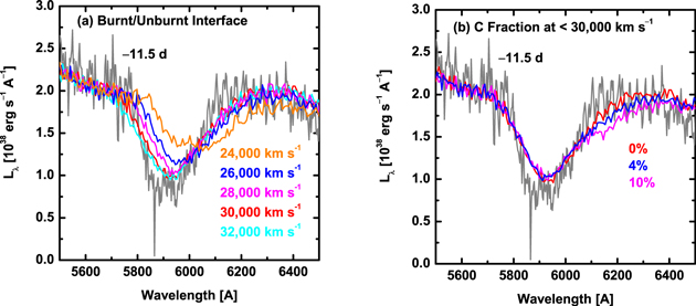
Figure 12. Comparison between the observed Si ii λ6355 at −11.5 days (gray line) and the synthesized spectra. The observed spectrum is corrected for the MW and the host galaxy extinction. (a) Shown here are models with different velocities at the interface between the burnt and unburnt layers. The dividing velocities are denoted in the figure legends. (b) Shown here are models with different mass fractions of carbon in the O–Ne–C burning layer. The three lines denote the 0%, 4%, and 10% for the carbon fraction, respectively.
Download figure:
Standard image High-resolution imageTo further constrain the amount of unburnt carbon below 30,000 km s−1, we also vary the mass fraction of carbon in the O–Ne–C burning layer (17,000–30,000 km s−1). The default value, 0% of carbon contamination, works well to reproduce the line profile on the red side. Note that while the carbon fraction is set constant within the O–Ne–C burning region, the constraint is basically placed at the region close to the photosphere, i.e., ∼20,000 km s−1. By increasing the C fraction, C ii starts to develop and suppress the emission component of Si ii (i.e., the red shoulder of Si ii). If X(C) is 10%, this effect is clearly seen in the model but not in the observed spectra, and thus we can place a conservative upper limit of ∼10% for the carbon fraction at ∼20,000 km s−1. Indeed, the effect is already distinguishable with X(C) ∼4%, which could also be regarded as the upper limit.
In summary, it is inferred that the outermost layers of SN 2019ein are structured as follows: (1) the O–Ne–C burning covers the region at least between 17,000 and 30,000 km s−1. The inner boundary can exist even deeper. (2) If the unburnt layer exists, its inner boundary is at least at 30,000 km s−1. (3) The mass fraction of unburnt carbon at ∼20,000 km s−1 is at most 4% (or 10% even as a conservative limit). (4) There is no mixing of deeper regions processed through more advanced nuclear burning out to the O–Ne–C burning/unburnt regions studied here.
4.3. Implications for Explosion Mechanism and SN Ia Diversity
The outermost layer of SN 2019ein can be well explained by the characteristic composition structure in the O–Ne–C burning layer found in the delayed detonation model. The (1D) delayed detonation model indeed predicts the velocity of this layer to be similar to that constrained for SN 2019ein: ∼15,000–27000 km s−1, ∼17,000–32,000 km s−1, and ∼19,000–35,000 km s−1 for the models CS15DD1, CS15DD2, and CS15DD3, respectively, in the model sequence of Iwamoto et al. (1999). The explosion mechanism of SN 2019ein is therefore well represented by the delayed detonation model. The nonexistence of the unburnt region up to at least 30,000 km s−1 is also consistent with the delayed detonation model. On the other hand, the same nucleosynthetic layer is confined in a small velocity range in the (1D) pure deflagration model W7 of Nomoto et al. (1984): ∼13,000–15,000 km s−1, with the unburnt layer at >15,000 km s−1.
Indeed, in the pioneering study of “SN spectroscopic tomography” by Stehle et al. (2005), they derived a similar composition pattern at ∼16,000–23,000 km s−1 for the prototypical HV SN 2002bo. They introduced a layer of a more (slightly) advanced burning stage in ∼23,000–27,000 km s−1, but this might not be robust; the first spectrum they modeled had the photospheric velocity decreasing to ∼16,000 km s−1. For SN 2019ein, we do not have to introduce such a composition inversion up to ∼30,000 km s−1. Given the uncertainty involved, we regard that the structure of the outermost layer of SN 2019ein shares similarities to SN 2002bo. This might therefore be a common property of HV SNe Ia.
NV SNe seem to have different characteristics in the outermost layer. For the best-studied NV SN 2011fe, the composition structure derived by Mazzali et al. (2014) shows that the O–Ne–C burning region is confined in the region at ∼13,300–19,400 km s−1 (with a slight mixing of more advanced burning products including 56Ni, which is not found for SN 2019ein). The region at >19,400 km s−1 is specified as an unburnt layer almost exclusively composed of carbon with primordial metals. By comparing their findings to those found for SN 2019ein in this work, we conclude that SN 2019ein has a more extended distribution of the O–Ne–C burning layer at higher velocities than SN 2011fe.
We note that SN 2019ein has a larger Δm15(B) than SN 2011fe, and it is supposed to be fainter with a smaller amount of 56Ni synthesized at explosion. Therefore, the amount of material processed by the most advanced burning (i.e., the complete Si burning) is seemingly smaller for SN 2019ein, despite the more extended distribution of the O–Ne–C burning region. This raises a challenge to the explosion mechanism, because there is generally a correlation between the extent of the 56Ni-rich region (or, the mass of 56Ni) and that of the O–Ne–C burning region in the explosion simulations. For example, this is clearly seen in the delayed detonation model sequence of CS15DD1-3 by Iwamoto et al. (1999), where the larger transition density leads to more extended regions both for the complete Si burning and O–Ne–C burning.
In the above discussion, we have mainly focused on the comparison between the properties of SN 2019ein and those expected by the delayed detonation model. Another explosion model that could also be consistent with our constraints is a pure-detonation model of a sub-Chandrasekhar mass WD. For example, such a model sequence by Sim et al. (2010) suggests that the region at ∼17,000 km s−1 is in the O–Ne–C burning region, which further extends to >20,000 km s−1, if the progenitor WD mass is below ∼1.1 M⊙. However, at the same time, the sub-Chandrasekhar WD explosion may be contaminated by the iron-peak elements at the highest velocity, in the scenario where the thermonuclear runaway of the sub-Chandrasekhar mass WD is triggered by the surface He detonation (i.e., a standard model for the sub-Chandrasekhar mass WD explosion; Fink et al. 2010); such a model would not satisfy the constraints placed by our present study.
5. Conclusions
In this paper, we present photometric and spectroscopic observations of HV SN Ia 2019ein starting 0.3 days (photometry) and 2.2 days (spectroscopy) since discovery. We estimate the explosion date as MJD 58602.87 ± 0.55, i.e., 1.6 days before the discovery, by fitting the expanding fireball model to the early rising multiband light curves. This places SN 2019ein as one of the best-studied SNe with the observational data starting within a few days since explosion.
The light-curve evolution shows that SN 2019ein is a relatively fast decliner with Δm15(B) = 1.36 ± 0.02 mag. The spectral indicators, i.e., the depth and relative pEW of Si ii λ6355 and Si ii λ5972, are consistent with Δm15(B). From the velocity of Si ii λ6355 and its evolution, it is robustly classified as an HV SN. In summary, SN 2019ein is an HV SN with relatively slow decline; this is a previously unexplored type of SNe Ia in terms of the observational properties starting within the first few days.
The earliest light curves are used to constrain the radius of a possible companion star for SN 2019ein. Similarly to other NV SN examples, we do not detect the excessive emission expected from a giant companion. Indeed, our multiband light curves are well fit by a single power law with an index of 2 (i.e., the fireball model).
The Si ii velocity around maximum light is modest for an HV SN; it is ∼13,000 km s−1. However, SN 2019ein shows the most rapid decrease in Si ii velocity toward maximum light among well-studied SNe Ia including both HV and NV SNe. It evolves more rapidly than those HV SNe showing the higher maximum-light velocity. It is most likely related to the rapid evolution in the light curves (i.e., large Δm15(B)). Namely, while it has been reported that the speed of the velocity decrease is correlated with the Si ii velocity around maximum light, this is not the whole story; the pre-maximum velocity evolution does depend on Δm15(B), not only on the velocity itself. Therefore, the velocity evolution of HV SNe does not form a one-parameter family.
This additional diversity may be further supported by the behavior in the early rising light curves. The rise time is suggested to be related to Δm15(B). HV SNe show generally shorter rise times than NV SNe for a given Δm15(B). The short rise time of SN 2019ein fits into the relation. Indeed, HV SN 2002er, with a similar Δm15 to SN 2019ein, showed a slow rise, opposite this relation. We note that the Si ii velocity of SN 2002er around maximum light is lower than 12,000 km s−1, which is among the lowest values to be classified as an HV SN. As such, it suggests that the velocity is indeed related to the light-curve behavior in the rising part.
We also provide spectral synthesis models for the earliest spectra taken within our program (3.7 and 5.7 days since the estimated explosion date). The phases are sufficiently early to place robust constraints on the nature of the outermost layer. The layer beyond ∼17,000 km s−1 is well described as the characteristic O–Ne–C burning region found in the standard (1D) delayed detonation model. Indeed, we do not find any evidence for mixing of more advance burning products from the deeper region. This region extends to at least 25,000 km s−1 (likely up to ∼30,000 km s−1), and there is no unburnt C + O material below ∼30,000 km s−1. This structure is similar to that derived for HV SN 2002bo, indicating that the basic structure of the outermost ejecta of HV SNe is not dependent on Δm15(B). The derived structure is very different from the structure of the outermost layer derived for the well-studied NV SN 2011fe, where the O–Ne–C burning region is found at much lower velocities and confined in a small velocity space. Given that the amount of material processed by more advance burning (e.g., 56Ni) should be larger for SN 2011fe than SN 2019ein, this might raise a challenge to the explosion mechanism. We suggest that the relation between the mass of 56Ni (or Δm15) and the extent of the O–Ne–C region provides an important constraint on the explosion mechanism(s) of HV and NV SNe.
This research has made use of the NASA/IPAC Extragalactic Database (NED), which is operated by the Jet Propulsion Laboratory, California Institute of Technology, under contract with the National Aeronautics and Space Administration. The spectral data of comparison SNe awere downloaded from the SUSPECT25 (Richardson et al. 2001) and WISeREP26 (Yaron & Gal-Yam 2012) databases. This research has made use of data obtained from the High Energy Astrophysics Science Archive Research Center (HEASARC), a service of the Astrophysics Science Division at NASA/GSFC and of the Smithsonian Astrophysical Observatory’s High Energy Astrophysics Division. This research made use of Tardis, a community-developed software package for spectral synthesis in supernovae (Kerzendorf & Sim 2014; Kerzendorf et al. 2019). The development of Tardis received support from the Google Summer of Code initiative and from ESA’s Summer of Code in Space program. Tardis makes extensive use of Astropy and PyNE. This work is supported by the Optical and Near-infrared Astronomy Inter-University Cooperation Program. Part of this work was financially supported by Grants-in-Aid for Scientific Research 17H06362 from the Ministry of Education, Culture, Sports, Science and Technology (MEXT) of Japan. This work was supported by the joint research program of the Institute for Cosmic Ray Research (ICRR). M.K. acknowledges support by JSPS KAKENHI Grant (19K23461). K.M. acknowledges support by JSPS KAKENHI Grant (18H04585, 18H05223, 17H02864). M.Y. is partly supported by JSPS KAKENHI Grant (17K14253). U.B. acknowledges the support provided by the Turkish Scientific and Technical Research Council (TüBİTAK-2211C and TüBİTAK-2214A).
Footnotes
- 17
We call the (lower-velocity) main absorption component the photospheric component following convention, although it does not have to be formed exactly at the photosphere.
- 18
IRAF is distributed by the National Optical Astronomy Observatory, which is operated by the Association of Universities for Research in Astronomy (AURA) under a cooperative agreement with the National Science Foundation.
- 19
- 20
- 21
The mean value of the results from different methods is μ = 32.20 ± 0.54 mag. A typical error associated with each measurement also exceeds ∼0.4 mag.
- 22
A possible contamination by HVFs is discussed in Section 3.4.
- 23
- 24
- 25
- 26