Abstract
While young stellar objects sometimes undergo bursts of accretion, these bursts usually occur sporadically, making them challenging to study observationally and to explain theoretically. We build a schematic description of cyclical bursts of the young stellar object EC 53 (also known as V371 Ser) using near-IR and submillimeter monitoring obtained over six cycles, each lasting ≈530 days. EC 53 brightens over 0.12 yr by 0.3 mag at 850 μm, by 2 mag at 3.35 μm, and by 1.5 mag at near-IR wavelengths, to a maximum luminosity consistent with an accretion rate of ∼8 × 10⁻⁶ M⊙ yr−1. The emission then decays with an e-folding timescale of  until the accretion rate is ∼1 × 10⁻⁶ M⊙ yr−1. The next eruption then occurs, likely triggered by the buildup of a ∼5 × 10⁻⁶ M⊙ mass in the inner disk, enough for it to become unstable and drain onto the star. Just before outburst, when the disk is almost replenished, the near-IR colors become redder, indicating an increase in the geometrical height of the disk by this mass buildup. The reddening disappears soon after the initial burst, as much of the mass is drained from the disk. We quantify physical parameters related to the accretion process in EC 53 by assuming an α-disk formulation, constrained by the observed disk properties and accretion rate. While we can only speculate about the possible trigger for these faithful eruptions, we hope that our quantified schematic will motivate theorists to test the hypothesized mechanisms that could cause the cyclical buildup and draining of mass in the inner disk.
1. Introduction
The accretion of gas through protoplanetary disks and onto pre-main-sequence stars is governed by the physics of gas instabilities, which allow some gas to gain angular momentum and travel outward, while other gas loses angular momentum and spirals inward (see reviews by Turner et al. 2014; Kratter & Lodato 2016). The efficiency of the instabilities changes with the physical conditions. Any spatial imbalance in disk dynamics, both locally and globally, must be balanced over long timescales.
When the accretion rate into the inner disk is higher than the accretion rate onto the star, gas will build up in some locations until that mass buildup overwhelms the blockage and drains onto the star through the magnetic field lines connecting the forming star to the disk. The consequence is a massive eruption of accretion onto the young stellar object (YSO). These accretion bursts typically are classified either as FUor objects (see the review by Hartmann & Kenyon 1996), for eruptions that persist for generations, or as EXor objects (Herbig 1989), for eruptions that persist for months.
For FUor objects, gravitational instabilities operating in the outer disk (10–100 au) may produce spiral density waves that propagate inward to (sub-)astronomical-unit regions, heat the disk, and trigger magnetorotational instability (e.g., Zhu et al. 2010b; Bae et al. 2013). In such a scenario, the outburst decay timescale can be approximated using the viscous timescale (Zhu et al. 2010a; Bae et al. 2014). Adopting a reasonable viscous parameter  , a decades-long decay suggests that the accretion instability is initially triggered at <1 au from the central star. For a viscous timescale, a decades-long decay indicates that the accretion instability is initially located at ∼1 au from the central star (Zhu et al. 2010b; Bae et al. 2014). The dynamical timescale for gravitational fragmentation and migration is much longer, 103–104 yr (Vorobyov & Elbakyan 2018), but the final act, where the fragments shear and accrete, is expected to occur in the inner few astronomical units (e.g., Nayakshin & Lodato 2012). For FU Ori, observational constraints yield an outer radius for the accretion disk R ≥ 0.5 au and a viscosity parameter α ∼ 0.1 when the decay timescale is ∼100 yr (Zhu et al. 2007).
For EXors, the instabilities are thought to occur at the magnetospheric boundary. Gas buildup in the inner disk may push the inner disk truncation radius closer to the star, eventually reaching a limit where that mass is quickly released onto the star (D’Angelo & Spruit 2010, 2012; Armitage 2016). The rise and decay timescales are both fast, typically ∼100 days (e.g., Herbig 1977; Aspin et al. 2010). Similar outburst events with even shorter timescales have been detected toward dwarf novae (see review by Osaki 1996).
Most EXors are known to repeat, though without consistency. The archetype, EX Lup, has eruptions every ∼20–30 yr (e.g., Herbig 2008). The EXor object VY Tau had a series of rapid eruptions and then became dormant (Herbig 1990). The long timescales for FUors mean that we do not have direct empirical evidence for repeated bursts. Although such large outbursts are very rare for optically bright stars (every 105 yr; Hillenbrand & Findeisen 2015; Contreras Peña et al. 2019), hydrodynamical models of accretion disks suggest that they may be more frequent in the early stages of stellar growth (e.g., Zhu et al. 2010b; Kadam et al. 2020). In some cases, periodic knots in outflows point back to historical episodes of accretion bursts (e.g., Reipurth 1989; Plunkett et al. 2015; Vorobyov et al. 2018; Matsushita et al. 2019; Lee 2020). For most YSOs, we have no ability to predict when a burst will occur.
In contrast to the apparently unpredictable timing of FUor and EXor accretion bursts, the YSO V371 Ser, hereafter EC 53 (Eiroa & Casali 1992), has faithful eruptions every ≈1.5 yr, allowing us to follow the rises and decays. EC 53 is located in the Serpens Main star-forming region at a distance of 436 ± 9 pc (Ortiz-León et al. 2017). We have been monitoring such cyclic eruptions and decays of the protostar EC 53 at submillimeter wavelengths as part of the James Clerk Maxwell Telescope (JCMT) Transient Survey (Herczeg et al. 2017; Yoo et al. 2017), and obtaining a wide array of supporting data to interpret these eruptions. EC 53 is empirically classified as a Class I object, based on a bolometric temperature of 130–240 K and a spectral index of 0.7–1 (Evans et al. 2009; Dunham et al. 2015). High-resolution Atacama Large Millimeter/submillimeter Array (ALMA) imaging indicates that the central object is a 0.3 M⊙ YSO having a 0.07 M⊙ disk (Lee et al. 2020) and surrounded by a 5.8 M⊙ envelope (Baek et al. 2020). This high envelope-to-(protostar+disk) mass ratio suggests that the source may be a Class 0 object. The innermost disk is viscously heated, with deep CO and H2O absorption lines in the near-IR that are characteristic of FUor objects (Connelley & Reipurth 2018; W. Park et al. 2020, in preparation).
The variability of the accretion onto the central star has been measured at JHK (Hodapp 1999; Hodapp et al. 2012) and submillimeter wavelengths (Mairs et al. 2017; Yoo et al. 2017) with periods consistent with ∼520–570 days. Modeling of the variation in the spectral energy distribution across a cycle uncovers a source bolometric luminosity ranging from 6 to 20  (Baek et al. 2020).
In this paper, we combine near-IR and submillimeter monitoring of EC 53 obtained over six cycles to establish a schematic picture of how intermittent accretion allows mass to build up in the disk until the dam breaks, releasing the gas and allowing it to accrete onto the star. We build this picture through regular photometric, broadband monitoring (Section 2) and analysis of periodicity in brightness and color variations (Section 3). Finally using the observed timescales for the near-IR rise and decay and an α-disk prescription, we quantify some of the physical phenomena in this picture and use those quantities to estimate physical parameters in the accretion disk (Section 4).
2. Observations and Data Reduction
We have been monitoring EC 53 at submillimeter wavelengths with the JCMT and in the near-IR with the United Kingdom Infrared Telescope (UKIRT), the Infrared Imaging Survey (IRIS) telescope, and the Liverpool Telescope. We have also obtained the light curve of EC 53 in the mid-IR (W2) from the Wide-field Infrared Survey Explorer (WISE) as complementary data. The date range and number of observations, by wavelength, are shown in Table 1.
Table 1. Data Set
| Telescope | Band (λ μm–1) | From | To | # Obs. |
|---|---|---|---|---|
| UKIRT | J (1.25) | 2014 Oct 12 | 2020 Feb 28 | 357 |
| UKIRT | H (1.63) | 2014 Oct 12 | 2020 Feb 28 | 359 |
| UKIRT | K (2.21) | 2014 Oct 12 | 2020 Feb 28 | 357 |
| Liverpool | H (1.64) | 2018 Mar 29 | 2020 Feb 16 | 71 |
| IRIS | J (1.24) | 2013 Jun 2 | 2017 Apr 25 | 31 |
| IRIS | H (1.66) | 2013 Jun 4 | 2017 Apr 25 | 38 |
| IRIS | Ks (2.16) | 2011 Mar 20 | 2019 Apr 14 | 85 |
| WISE | W2 (3.35) | 2014 Mar 31 | 2018 Sep 8 | 20 |
| JCMT | 850 | 2016 Feb 3 | 2020 Feb 22 | 50 |
| JCMT | 450 | 2016 Feb 23 | 2020 Feb 22 | 31a |
Note.
aThe smaller number of data points as compared to 850 μm is due to the greater dependency on atmospheric emission and weather (see Section 2.1).Download table as: ASCIITypeset image
In this section we describe the observing strategies of the various near-IR, mid-IR, and submillimeter observations used in this paper. Further details of the observations are included in the appendix.
2.1. The JCMT Transient Survey
SCUBA-2 (Holland et al. 2013) continuum observations at 450 and 850 μm were obtained simultaneously as part of the JCMT Transient Survey (project code: M16AL001; Herczeg et al. 2017). The Pong 1800 observing mode (Kackley et al. 2010) was used to yield a map with a uniform sensitivity over a 30′ diameter circular region centered at (R.A., decl.) = (18:29:49, +01:15:20, J2000). This region was observed approximately monthly (depending on weather conditions and source availability) since the first observation on 2016 February 2 (UTC). The integration time of each observation was varied to ensure a consistent background noise level of ∼10 mJy/beam at 850 μm (Mairs et al. 2017). The 450 μm background noise level varied greatly as it is much more dependent on submillimeter emission from the Earth’s atmosphere than the 850 μm data. The 450 μm and 850 μm beam sizes were 96 and 14
1, respectively (Dempsey et al. 2013).
The JCMT submillimeter flux measurements were converted to magnitudes using the following scaling:

where Z850 = 1.04 Jy/beam and Z450 = 3.58 Jy/beam.
2.2. Near-infrared Data
In the near-IR, JHK, EC 53 appears as a compact but resolved source (with an FWHM of around 2″ in the H band) and a nebula that fans out southeastward (e.g., Hodapp 1999). The compact source must contain both the variable EC 53A and its nearby (03 distant) apparently constant companion EC 53B (Hodapp et al. 2012). The nebula can be traced out to about 20″ in 360 s of H-band exposure with the Liverpool Telescope, and presumably extends all the way to the terminal shock S11 an arcminute away (Herbst et al. 1997; Hodapp et al. 2012).
We observed EC 53 using the 3.8 m UKIRT, Hawaii, and the UKIRT Wide Field Camera (WFCAM; Casali et al. 2007). WFCAM employs four 2048 × 2048 HgCdTe Hawaii-II arrays, each with a field of view of 1365 × 13
65 at an image scale of 0
4 per pixel. The target was placed on array #3 of WFCAM during all observations. Monitoring observations were obtained at the J, H, and K bands during a period of over 5 yr from 2014 October 12 to 2020 February 28.
We also obtained J-, H-, and Ks-band imaging photometry of EC 53 with the IRIS 0.8 m telescope (Hodapp et al. 2010) and 1024 × 1024 2.5 μm IRIS IR camera of Universitätssternwarte Bochum on Cerro Armazones, Chile. The observations were part of a long-term monitoring program of the Serpens NW star-forming region. In the J-, H-, and Ks-band filters, the integration time per exposure was 20 s, and for each observation, 10 such frames were obtained, as well as 10 frames on a separate sky position. The data reduction pipeline produced dark-subtracted, flat-fielded, sky-subtracted, and co-added images with a pixel scale of 0375 per pixel. The photometry was extracted using the IRAF task APPHOT with an aperture of 22 pixels = 8
25 diameter. The photometry was calibrated against a set of Two Micron All Sky Survey stars selected to be isolated, sufficiently bright, and non-variable.
We obtained further IR observations of EC 53 using IO:I (Barnsley et al. 2016) on the Liverpool Telescope (Steele et al. 2004) on the island of La Palma in the Canary Islands. The Liverpool Telescope observed a full light curve for one periodic cycle. Given the extended source structure it is not clear what size aperture is optimal for IR photometry with the Liverpool Telescope. We therefore experimented with 13, 3
7, and 5
2 radius apertures using the H-band data. By subtracting the magnitudes in these different apertures we found that the variations between them were less than ±0.05 mag rms. We therefore settled on using a 3
7 radius aperture, which is greater than the worst seeing but still minimizes the effect of the nebula, for all our IR data. To bring the heterogeneous data sets into alignment, we added an offset to all Liverpool H-band data points. The offset value was optimized by the minimum string length method (Dworetsky 1983) with the combined light curve of UKIRT H and Liverpool H after adding the offset (see Section 3.1 for details about the minimum string length method).
2.3. Mid-infrared Data
WISE (Wright et al. 2010) is a 40 cm telescope in a low Earth orbit that has surveyed the entire sky using four IR bands centered at 3.4, 4.6, 12, and 22 μm (bands W1, W2, W3, and W4) and with an angular resolution of 61, 6
4, 6
5, and 12
0, respectively. The orbit of WISE allows it to cover every part of the sky at least eight times (Mainzer et al. 2011), with each patch of sky observed many times over a period of ∼1 day. The original survey ran between 2010 January and September. Once the telescope’s cryogen tanks were depleted it continued to operate for 4 months using the W1 and W2 bands (known as the NEOWISE Post-cryogenic Mission; Mainzer et al. 2011). The NEOWISE mission was reactivated in 2013 (Mainzer et al. 2014) and has continued to operate since.
In this work we explored the NEOWISE single-exposure database (2019 data release), which contains W1 and W2 observations from 2013 December to 2018 December (Cutri et al. 2015). The NEOWISE single-exposure detections are complete up to W1 = 15 mag and W2 = 13 mag (Cutri et al. 2015).
3. Light Curves
Figure 1 presents the near-IR and 850 μm light curves for EC 53 across six cycles of brightening and decay. The light curves in the J, H, and K bands show abrupt brightening on a short timescale, followed by a slow decline. This pattern is characteristic of YSO outbursts (e.g., Bell et al. 1995; Audard et al. 2014). For EC 53, the amplitudes of luminosity changes are smaller than those of FUors and EXors; the duration of bursts for EC 53 is similar to that for EXors, but the bursts of EC 53 are distinguished from others by their regularity. The variation across the periodic cycle is ∼1.5 mag (∼4 in flux) in the near-IR and ∼0.3 mag (∼1.5 in flux) at 850 μm. In Figure 1 the change in magnitude at 850 μm has been increased by a factor of 5.5, with a vertical shift for easy comparison (see also Section 3.5).
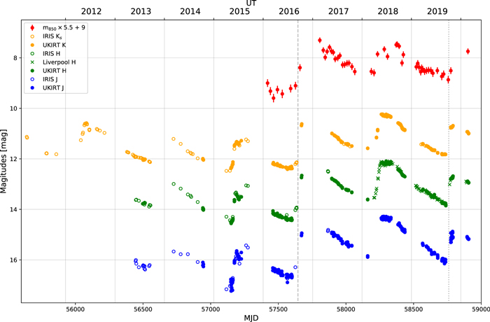
Figure 1. Light curves of EC 53 at near-IR and 850 μm bands (see the legend for detailed information). The submillimeter-band magnitudes are arbitrarily scaled by 5.5 and offset by 9 mag to facilitate comparison. The horizontal axes show the modified Julian date (MJD = JD–2,400,000.5) below and the years in Universal Time (UT) on top. The dashed line at MJD = 57,640 (2016 September 9 in UT) denotes where EC 53 becomes brighter by about a magnitude in the near-IR. The dotted line at MJD = 58,760 (2019 October 4) denotes where EC 53 becomes fainter by about half a magnitude in the near-IR.
Download figure:
Standard image High-resolution imageIn addition to the cyclical accretion bursts, the near-IR light curve shows a long-term brightness increase. The faintest and the brightest phases in the cycle were both brighter in 2019 than in 2015.
3.1. Period Determination
To quantify the time dependence of the observed brightness variations, we calculate the period of each light curve using the phase-folded diagram string length method. The string length method (Dworetsky 1983) searches for the period that produces the smoothest phase-folded diagram waveform by minimizing the string length, where the measured length is the sum over the line segments connecting successive points in phase order. We modify the string length method to search for the best-fit offset as well as the best-fit period, recognizing the long-term brightening of the underlying system of EC 53.
We compensate for the overall brightening of the object by increasing the brightness obtained earlier than 2016 September 9 and after 2019 October 4. For each near-IR band, we test brightness offsets between 0 and 1.5 mag, with 0.01 mag intervals, and periods from 500 to 600 days, with 5 day intervals. The modified string length method yields a best fit of 530 days each for J, H, and K. We find 570 days for the 850 μm observations, which are likely affected by the time baseline (see Section 3.4 and Appendix B).
For the data points before 2016 September 9, the best-fit offsets are 1.01, 0.96, and 0.78 mag for J, H, and K, respectively. For the data points after 2019 October 4, we optimize the offset value required to bring the phase curve into agreement. The applied offsets are 0.6, 0.55, and 0.44 mag for J, H, and K, respectively. At 850 μm the offsets are 0.74 mag before 2016 September 9 and 0.24 mag after 2019 October 4, which are applied after the scaling of 5.5 shown in Figure 1.
For completeness, in Appendix B we present a more thorough analysis of the light curves by using periodogram and autocorrelation methods, with and without brightness offsets for the data obtained prior to 2016 September 9 and after 2019 October 4.
3.2. Phase-folded Diagram Analysis
In this section we use only epochs with corresponding JHK measurements in order to evaluate the color of EC 53 as a function of phase. Following our results in Section 3.1, we draw the phase-folded diagrams of the light curves in the near-IR and at 850 μm with a 530 day period. We also present the near-IR color as a function of phase. We adopt the same period at every wavelength because the periodicity of the system should be independent of wavelength. Given that our analysis covers roughly three full periods, an uncertainty of less than a few percent in the phase ( days) introduces little phase scatter. The phases are aligned such that the observed minimum in the near-IR occurs at phase 0.5. Our goal in this section is to uncover gross changes in the physical properties of the system with phase.
3.2.1. Phased Light Curves
In the near-IR, the brightness sharply increases starting at phase 0.5, reaches the peak at phase ≈0.6, and decays slowly (Figure 2; note that in the figure we show two complete periods). In the submillimeter band, the brightness increase and decrease appear much more symmetric. Although the submillimeter data points have a large scatter, the initial submillimeter decay stops earlier (phase ≈0.25) than the near-IR drop. The submillimeter rise occurs at roughly the same time as the near-IR rise (phase ≈0.5), but more gently than the near-IR rise; this might suggest that the submillimeter peak is delayed with respect to the near-IR.
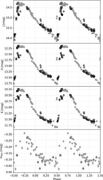
Figure 2. Phase-folded diagrams using 530 day period at J, H, K, and 850 μm (top to bottom). Observations before 2016 September 9 and after 2019 October 4 have been scaled up by the fixed values at each wavelength (see text) and are marked with dark black circles and black squares, respectively.
Download figure:
Standard image High-resolution imageA significant phase-dependent color variation is also observed (Figure 3). A reddening of the source begins at the same time that the submillimeter curve stops declining (phase ≈0.25), leading to a sharp reddening peak and decline around phase ≈0.6, during the observed brightening of EC 53 in the near-IR. After this abrupt reddening event the color of the source gradually becomes bluer until phase ≈1.
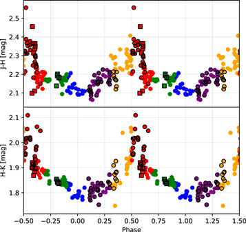
Figure 3. Same as Figure 2 but showing the near-IR colors (J − H and H − K). The symbols used in the plot are tinted to indicate phases of −0.1 to 0.1 (blue), 0.1 to 0.3 (purple), 0.3 to 0.5 (yellow), 0.5 to 0.7 (red), and 0.7 to 0.9 (green).
Download figure:
Standard image High-resolution imageThe well-sampled color–phase curve reveals an extreme reddening coincident with the abrupt start of each burst. Independently of phase, the near-IR colors of EXors and FUors span a wide range, with J − H = 0.5–3. The color variation observed for EC 53 is distinct from the typical trend found in EXors, which have bluer near-IR colors around the burst and redder colors during the quiescent phase (Kóspál et al. 2011; Lorenzetti et al. 2012). For FUors the observed color variations are more diverse. HBC 722 shows color variation similar to that of EXors (Kóspál et al. 2011) even though the source is classified as an FUor in recent photometric (Connelley & Reipurth 2018) and spectroscopic studies (Lee et al. 2015). The colors of V1057 Cyg and V960 Mon follow an extinction law in the optical band during the decay, right after the peak brightness (Kopatskaya et al. 2013; Hackstein et al. 2015). On the other hand, V346 Nor becomes redder during its slow brightening (Kóspál et al. 2020).
3.2.2. Phased Color–Magnitude Diagrams
To diagnose the cause of the flux and color variation we produce color–magnitude diagrams for the near-IR (Figure 4). Starting at phase ≈−0.25 (green points), the source becomes sharply fainter and slightly bluer. From phase ≈0.25 to phase ≈0.5 (purple and yellow points) it continues to fade but becomes much redder, roughly following the reddening law in typical interstellar matter (Cardelli et al. 1989). The reddening trend in the H band (lower panel of Figure 4) appears flatter than the J-band photometry. Such a flattened trend occurs when the source is reddening and intrinsically brightening simultaneously, which gives insight into the timing offset of the brightening between the near-IR and the submillimeter band (discussed in Section 4). Around phase ≈0.5 (yellow and red points) the source rapidly increases in brightness while staying red. After the abrupt rise in brightness, the source continues to brighten and get bluer, following the reddening law in reverse (red and green points). The source then begins to dim once more (blue points) as the cycle repeats.
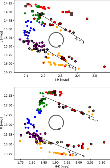
Figure 4. (J − H) vs. J (upper) and (H − K) vs. H (lower) color–magnitude diagrams. The symbols are tinted to indicate the phase following the scheme defined in Figure 3. The black arrows in the diagrams are the reddening vectors (Cohen et al. 1981), corresponding to (Av = 3 or −3) as indicated in the plot. The counterclockwise direction of the vectors follows roughly the phase order of the data points.
Download figure:
Standard image High-resolution image3.3. Near-infrared Decay and Rise Timescales
To measure the decay and rise timescales, we fit a linear function to the decaying and rising sections of the Liverpool Telescope H-band light curve (Figure 5). The measured slopes are 1.47 ± 0.01 mag yr−1 for the dimming and −11.9 ± 0.1 mag yr−1 for the brightening. We convert the slope, n, to the timescale of luminosity variation, τ, as follows:

Here, m0 and L0 are the initial magnitude and luminosity, respectively. Thus,

and to determine the timescale in which the luminosity changes by a factor of e,

This reduces to the convenient form, τ ≈ 1.086/n. Therefore, the decay timescale of EC 53 in the H band is ≈0.74 yr, an order of magnitude longer than the brightening timescale of ≈0.091 yr.
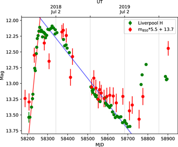
Figure 5. Light curve at H band from the Liverpool Telescope and at 850 μm from the JCMT. The 850 μm magnitudes are arbitrarily adjusted (multiplied by 5.5 and offset by 13.7 mag) for easier comparison.
Download figure:
Standard image High-resolution imageWe overlay the H-band rise and decay slopes measured for a single cycle with the Liverpool Telescope on the full H-band light curve in Figure 6. Each individual rise and decay is well fit with the value derived above, but the timing between the rise and decay shows some variability, indicating an inherent fluctuation within the apparent periodicity of the system.
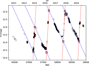
Figure 6. The H-band light curve of UKIRT (black circles), with the additional data obtained from the IRIS telescope (gray circles) and Liverpool Telescope (gray crosses). The red and blue lines are the linear fit to the most recent observed period (Figure 5), duplicated to the other periods. The crossing points of the slopes are denoted as black squares.
Download figure:
Standard image High-resolution image3.4. Perturbation in Periodic Cycle
As discussed in Appendix B, the period of EC 53 does not clearly converge to a single value but depends on the time when the observations are taken. The phase-folded diagrams (Figures 2 and 3) also show apparent scatter with respect to a single period.
Measured from Figure 6, the offset times between the observed fadings of EC 53 are 450, 760, and 550 days (blue lines), while the rises are separated by 460, 560, and 550 days (red lines). The time displacement between the crossing points (black squares in Figure 6) indicates the hypothetical maximum and minimum points, with displacements of 459, 582, and 550 days (left to right).
3.5. Mid-infrared and Submillimeter Scaling
The variations in the mid-IR and 450 μm light curves are consistent with those seen at 850 μm (Figure 7, left panel), though with fewer data points. We perform an orthogonal distance regression to derive the scale factor and offset that give that best agreement between the magnitudes of two different wavelengths. Between the 850 μm and W2 bands, we uncover a scale factor of 6.1 ± 0.5 and an offset of 8.44 ± 0.01 (Figure 7, upper right panel). The best fit for the 850 μm and 450 μm magnitudes yields a scale factor of 2.2 ± 0.1 and an offset of −0.2 ± 0.004 (Figure 7, lower right panel).
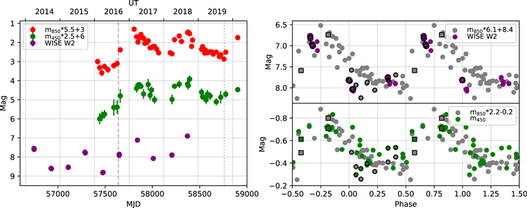
Figure 7. Light curves (left) and phase-folded diagrams at 850 μm, 450 μm, and WISE W2 bands. The light curves of the submillimeter bands are arbitrarily scaled (see legend). Phase-folded diagrams (right) showing 850 μm against WISE W2 band (top) and 450 μm (bottom) with the required scaling factor for agreement.
Download figure:
Standard image High-resolution imageContreras Peña et al. (2020) measured a scaling factor of 5.5 ± 0.3 between the submillimeter and mid-IR magnitudes in a sample of a dozen protostars, including EC 53, which simultaneously varied at both wavelengths. The fitting from a single burst of EC 53 was 6.18 ± 0.65. In that paper, the submillimeter to mid-IR correlation was interpreted as the variation of mid-IR emission roughly tracing the underlying bolometric luminosity of the source, and the varying submillimeter emission tracing more closely the dust temperature within the envelope. Additional evidence in favor of the luminosity/dust temperature explanation for the tight correlation and scaling has been found through radiative transfer analyses and spectral energy determinations of modeled embedded sources, both analytic and numeric, with varying central luminosities applied (MacFarlane et al. 2019a, 2019b; Baek et al. 2020).
The measured stronger response to brightness changes at the shorter submillimeter wavelength is also expected, as the 450 μm emission probes somewhat closer to the peak of the dust spectral energy distribution produced by the protostellar envelope (see, for example, MacFarlane et al. 2019a, 2019b; Baek et al. 2020). The detailed radiative transfer modeling in those papers, however, reproduced a scale factor <2, suggesting that there are still aspects of the protostellar models that require refinement.
4. Discussion
In this section we combine the observational attributes from the near-IR and submillimeter monitoring to build a schematic picture of the accretion bursts and fades of EC 53, summarized in Figure 8 and Table 2. Using this framework we measure relevant quantities directly from the observations and analyze them using a simple α-disk formalism to estimate reasonable physical properties of the inner disk dynamics. This prescription is not meant to be definitive but rather to examine quantitatively the physical requirements of the system such as the basic disk properties required to produce the bursts and fades of EC 53. We finish with a plausible toy model that recreates each of the observed features.
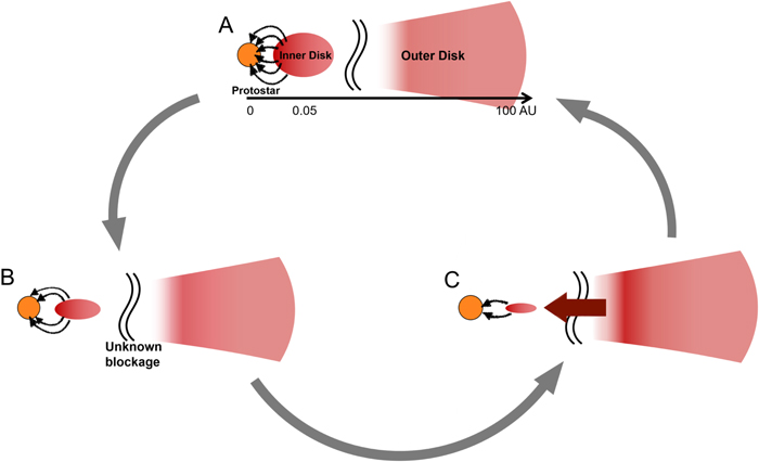
Figure 8. Schematic view of the EC 53 system. A: The inner disk, at its fullest and thickest (phase = 0.5), begins accreting onto the central protostar. The protostar and inner disk brighten rapidly as the viscous inner disk spreads (phases 0.5–0.7). Nevertheless, the source appears reddest due to extinction produced by the puffed disk. B: Losing mass to the central protostar, the inner disk becomes thinner, the extinction lessens, the observed emission becomes less red, and the accretion rate declines (phases 0.7–1 and 0–0.3). During this stage material from the outer disk is blocked from replenishing the inner disk. C: Held-back material from the outer disk quickly falls onto the inner disk during this short stage (phases 0.3–0.5), priming the system for the next cycle.
Download figure:
Standard image High-resolution imageTable 2. Description of the Cycles of EC 53
| Phase | Empirical Diagnostic | Physical Interpretation | Role in Schematic Picture |
|---|---|---|---|
| 0.5–0.7 | Brightness increase | Rapid increase in accretion rate | Disk starts draining |
| ≈0.7 | Maximum brightness | Maximum accretion rate | Peak of mass release from inner disk |
| 0.7–1.0, 0.0–0.3 | Brightness decay | Decreasing accretion rate | Draining of the inner disk |
| ≈0.1 | Bluest near-IR colors | Lower extinction | Lower disk height from draining inner disk |
| 0.3–0.5 | Near-IR colors increase | Increasing extinction | Disk height gets larger as inner disk fills |
Download table as: ASCIITypeset image
4.1. Decay Time and Associated Viscous Time
In Section 3.3 the exponential decay rate of the near-IR brightness is measured as 0.74 yr for the most recent decline, using the Liverpool Telescope data set (Figure 5). This decay rate fits very well the previous decays after burst (Figure 6). Thus, it appears that the timescale has a physical origin, which we associate with a viscous spreading time in the accretion disk surrounding the protostar,  . Within order unity (Hartmann et al. 1998),

where

and R0 is the characteristic size of the accreting disk, H0 is the scale height of the disk at R0, cs is the sound speed in the disk, and  is a scaling parameter for the viscosity (see, e.g., Shakura & Sunyaev 1973; Matsuyama et al. 2003).
Rearranging, we obtain an equation for the characteristic size of the accreting disk:

After substitution of fiducial values, we find

Thus, it is possible to associate the decay time with the viscous time in the innermost region of the circumstellar disk, where enhanced accretion is taking place. This requires, however, both a very small inner accretion disk,  (10 R⊙), and a very high viscosity parameter, α ∼ 0.3. We note that this α value is higher than the typical value accepted for FU Ori, ∼0.2–0.02 (Zhu et al. 2007).
4.2. Mass Accretion during Burst
The amount of material accreted onto the protostar during a single burst can be determined directly from the bolometric light curve, under the assumption that the observed brightness is due to released accretion energy (Hartmann 2009). Taking a mass of EC 53 of  (Lee et al. 2020) and assuming a radius of
  , we estimate a mass accretion rate of

where η ≤ 1 captures the uncertainty in the fraction of energy radiated away during accretion. It is anticipated that η ∼ 1 (see Hartmann et al. 2011 for a discussion).
The observed exponential decay rate of the near-IR brightness suggests a similar relationship of luminosity versus time,

with  (Baek et al. 2020). Substitution into Equation (9) and integration over the length of the observed decay,
  yr, we find



With η ∼ 1, the maximum accretion rate is  , significantly higher than the values typically measured for Class I sources from direct accretion diagnostics (e.g., White & Hillenbrand 2004; Salyk et al. 2013) or from bolometric luminosities (Dunham et al. 2010; Fischer et al. 2017) and even greater than the expected steady-state accretion value for a young, Class 0/I protostar forming over ∼0.5 Myr.
4.3. Inner Disk Mass
In the preceding sections we have assumed that a viscous inner accretion disk is responsible for the accretion of material onto the protostar. Thus, applying α-disk constraints (e.g., Hartmann et al. 1998), we estimate the required surface density,  , in the inner accreting disk:


Rearranging this yields

Furthermore, assuming steady-state α-disk conditions yields  and therefore



Thus, the mass of the inner accretion disk is only 2.3 times as large as the total amount of material accreted during a single episodic event suggesting that an outer disk reservoir is required to replenish the inner accretion disk.
4.4. Outer Disk Conditions
While the inner disk is observed to accrete material onto the protostar episodically, we have shown in the preceding section that there must be replenishment from the outer disk in order for the bursts to recur. If we assume that accretion through the outer disk is steady, then


Thus, even our assumed steady-state mass accretion rate in the outer disk reflects better anticipated Class 0 conditions versus Class I expectations.
Furthermore, the outer disk mass is estimated as  by Lee et al. (2020), assuming standard conversions between millimeter-continuum emission and mass. If the outer disk has a surface density
  , then

Starting with a large disk,  au (Lee et al. 2020), we extrapolate this outer disk mass to the scale of the inner accretion disk where
  au, finding
  . This result is approximately 130 times the above-determined mass of the inner accretion disk (Section 4.3).
We thus conclude that while the outer disk has plenty of mass available near its inner edge, it is unable to smoothly supply the inner disk with material. An accretion blockage occurs somewhere beyond the inner disk,  au, where the inwardly accreting material from the outer disk is held up. The blockage is only temporary, however, and after ≈1.5 yr the stored material is released and quickly drains onto and through the inner disk.
An additional consequence of this model is that the effective α value for the inner part of the outer disk is significantly lower than that for the inner disk. Assuming that the quantity  does not vary significantly across the inner and outer disk boundary then the ratio of α is inversely proportional to the local surface density scale factor (see Equation (14)), implying that in the outer disk α ∼ 0.002.
4.5. Replenishment Time and the Extinction Event
From the near-IR light curve we find an exceptionally fast exponential rise time to the peak brightness:  yr. Before the near-IR rise, however, we observe enhanced reddening of the source, which we associate with a strong extinction event (Figure 3). The extinction begins around phase 0.25 and becomes extreme near phase 0.5. The full reddening event persists for ≈0.4 yr, although the most extreme (
 ) reddening lasts for only ≈0.1 yr.
If the material partaking in each individual burst is held up in the outer disk and then released, rapidly falling to the inner disk, then the fastest timescale available would be the dynamical time. For a  protostar, a 0.1 yr infall timescale corresponds to a distance of R ∼ 0.4 au. This scenario requires both a mechanism for holding back the outer disk accretion at ∼0.4 au, and a release mechanism that streams the material directly into the inner disk. Despite these complexities, an intriguing aspect of this scenario is that the burst periodicity,
  yr, is only a few times the local Keplerian orbital time in the disk where the material is required to be held up (the freefall time is 0.18× the orbital time).
Alternatively, the viscous and accreting outer disk might be efficient to well inside 0.4 au but might become hung up closer to the measured size of the inner disk, 0.05 au, with the effective viscosity at this boundary decreasing steeply such that α ≪1. In this scenario the increased mass buildup near the inner disk boundary takes place over many local Keplerian revolutions, eventually reaching a tipping point during which the effective viscosity rises sharply such that α ∼ 0.3. We note that the physical plausibility of this scenario requires theoretical validation as the effective viscosity has to change dramatically over very short timescales.
The physical cause for the cycles of bursts and blockages is uncertain. Explanations for accretion bursts include magnetospheric instabilities in the inner disk (e.g., D’Angelo & Spruit 2010), gravitational instabilities near the star (e.g., Bae et al. 2014), and interactions between the disk and a close companion (e.g., Bonnell & Bastien 1992; Nayakshin & Lodato 2012; Muñoz & Lai 2016).
The disk fragmentation scenario (e.g., Vorobyov & Basu 2010) is especially intriguing for EC 53 given the estimated disk mass to protostar mass ratio of ∼0.25. This scenario, however, places the fundamental instabilities in the outer disk and would probably require longer timescales than measured for EC 53, although the migration of clumped material from the outer disk might be responsible for triggering an instability within the inner disk (Nayakshin & Lodato 2012).
Of all the possible explanations, the planet or companion hypothesis suggested by Hodapp et al. (2012) and Yoo et al. (2017) is the only one that would specifically invoke quasi-periodic behavior.
Several other outbursts found in the literature have been analyzed for their triggering mechanisms. The mid-IR outburst of Gaia 17bpi preceded the optical outburst, implying an outside–in event where the disk heated prior to accretion onto the central star (Hillenbrand et al. 2018). The outburst event of the Class I object Gaia 19ajj showed extinction from color variation in the mid-IR (Hillenbrand et al. 2019). FU Ori itself may have a constant replenishment of its inner disk (Liu et al. 2019), leading to a smooth light curve for almost a century. Dwarf novae, which undergo repetitive observable outbursts, allow for monitoring and provide considerable references (Osaki 1996). For example, theoretical models have been used to investigate the hysteresis observed in the time-dependent color–magnitude diagrams of some dwarf novae, attempting to fit simultaneously emission from the star, the accretion hot spot, and the disk with moderate success (Hameury et al. 2020). Unlike the hysteresis seen in the color–magnitude diagram for EC 53 (Figure 4), where the change in color with phase appears to be due to a changing extinction, for dwarf novae the optical color change is interpreted as either a variation in the temperature of a component or a change in the relative brightness between components.
Previous studies typically focus on the burst, while in this paper we also demonstrate the relevance of the blockage. In the schematic picture described here (Table 2 and Figure 8), this blockage is understood as a change in the disk viscosity from high α in the innermost regions to low α in the outer regions. While our derived absolute value of α for the inner disk is significantly larger than normally assumed, its ratio against the estimated outer disk α indeed satisfies this requirement.
An alternative possibility invokes changes in the mass-loss rate or pressure within the wind to destabilize disk accretion. Lee et al. (2015) demonstrated that wind pressure prevents the refilling of the disk when accretion is strongest for the early phase of the FUor burst of HBC 722.
Whatever the specific physical causes of the bursts and blockages, they must explain the rise and decay cycles, and the generic picture of the inner disk that we have derived from analyzing those cycles.
4.6. Toy Model to Explain the Observations
Utilizing the observational evidence presented in the preceding section (Section 3) we build here a simple toy model for the near-IR and submillimeter light curves of EC 53. We begin by assuming that the accretion-dominated bolometric luminosity light curve is composed of two coupled exponential functions:

where ϕ is the phase (between 0 and 1),  is the offset required to match the observed phase-folded diagram (Figure 2), and the coefficients in the exponential functions reproduce a decay time of 0.74 yr (
 ) and a rise time of 0.2 yr (
 ) when scaled to the 1.5 yr period of the system. We further assume that the unattenuated near-IR luminosity scales with the accretion luminosity such that



where the nonlinear scaling is meant to create a slight color variation with changing source luminosity such that the unattenuated light from the system is somewhat bluer when least luminous.
The submillimeter brightness is dominated by emission from dust in the extended obscuring envelope surrounding EC 53, which has a delayed reaction of up to a couple of months to changes in the accretion luminosity due to the light-crossing time (Johnstone et al. 2013) for an envelope size of 10,000 au (Baek et al. 2020). To simplify the computation for this model, we calculate the submillimeter flux by averaging the dust temperature response over δϕ = 0.2 and delaying it by  (0.15 yr). The top panel of Figure 9 shows the resultant magnitude light curve at the H band and in the submillimeter band (after rescaling). Due to the smoothing and delay, the submillimeter light-curve extrema lag those in the unattenuated near-IR light curve at all phases.
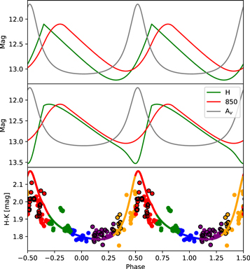
Figure 9. The light curves and color curve from the toy model. The top and middle panels show the H-band, submillimeter, and extinction curves. The top panel shows the original light curve of the H band and the middle panel shows the light curve after applying extinction. The bottom panel presents the color curve of H − K from the toy model (line) with the observation (circles).
Download figure:
Standard image High-resolution imageThe observational data also reveal a strong reddening event just after the submillimeter emission begins to rise (Figure 3), which we associate with enhanced extinction. For the toy model we represent the extinction event as a localized event, using the following equation:

where the maximum extinction takes place at  and γ = 0.1.
The effect of the extinction event on the observed near-IR magnitudes is thus



where the coefficients in front of the exponent reproduce the expected reddening law due to extinction (Cohen et al. 1981).
The middle panel of Figure 9 shows the resulting light curves. The submillimeter rise is now advanced with respect to the H band, entirely due to the addition of the near-IR extinction event. The submillimeter peak remains somewhat delayed due to the imposed propagation lag through the extended envelope. These features in the model light curves are now in agreement with the observations. Furthermore the H-band rise has become significantly steeper than the submillimeter rise, which occurs at the same time as the extinction event. As compared with the observations, the most significant departure in the light curve produced by the toy model is the enhanced dip at the end of the H-band decay. In the observations the decay appears smoother, suggesting that the functional form for the extinction event is not quite appropriate. The bottom panel of Figure 9 shows the H − K color for the toy model, again reasonably reproducing the observations.
The toy model color–magnitude diagrams are reproduced in Figure 10. In both panels we include measurements with a two-week cadence in order to show the time spent in each part of the cycle. The overall appearance of the panels matches the observations, despite significant differences in details.
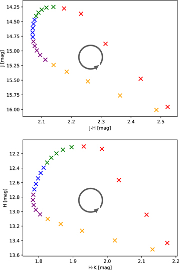
Figure 10. Color–magnitude diagrams obtained from the toy model. The color of the markers is tinted as in Figure 9.
Download figure:
Standard image High-resolution image5. Conclusions
This paper summarizes our understanding of the eruptions and fades of EC 53. This cycle faithfully repeats every ≈530 days, in contrast to the apparent stochasticity of explosions in other eruptive YSOs. This predictability has motivated us to intensely monitor EC 53 in the submillimeter and near-IR bands, supplemented by high-resolution ALMA imaging and high-resolution near-IR spectroscopy as well as radiative transfer modeling.
In our schematic interpretation of EC 53, steady accretion from the outer disk to the star is not possible. Thus, mass builds up somewhere within the inner 0.4 au of the disk. After about 1.5 yr the blockage becomes unstable, draining into the inner disk and onto the star. This scenario is similar to that described by Banzatti et al. (2015) for the accumulation and release of mass in the EX Lup disk, as measured from H2O, CO, and OH line emission (see also Goto et al. 2011). For EC 53, the total mass accreted during a burst is  M⊙, about half of the total mass of the inner disk. Furthermore, the rise and decay e-folding timescales are always the same, indicating consistent physical explanations between epochs, despite some stochasticity in timing and amount of material accreted.
The buildup of material would lead to a larger geometric height of the disk, consistent with the increased extinction. This explanation is similar to associations between increased accretion and extinction sometimes seen in FUors (e.g., Kopatskaya et al. 2013; Hackstein et al. 2015; Hillenbrand et al. 2018, 2019). For EC 53, the extinction increases sharply around the peak luminosity, and then disappears quickly as most of the material is drained, leading to a geometrically smaller disk.
Our schematic picture places strong, generalized constraints on the physical mechanisms that cause the cycles of eruption and decay for EC 53. The inner disk must be highly viscous to facilitate such high accretion rates to drain most of the inner disk. The inner disk must be replenished sufficiently to trigger a burst 525 days later, from a region in the disk with a lower viscosity. We hope that this schematic picture motivates investigation into the companion and/or instability physics that may cause the repeated eruption and decays of YSOs.
We thank the anonymous referee for thoughtful comments that helped to improve this paper. This work was supported by the Basic Science Research Program through the National Research Foundation of Korea (grant no. NRF-2018R1A2B6003423) and the Korea Astronomy and Space Science Institute under the R&D program (project No. 2020-10-840-06) supervised by the Ministry of Science, ICT, and Future Planning. D.J. is supported by the National Research Council of Canada and by an NSERC Discovery Grant. T.N. and C.C.P. were supported by a Leverhulme project grant. G.J.H. is supported by general grant 11773002 awarded by the National Science Foundation of China.
UKIRT is owned by the University of Hawaii (UH) and operated by the UH Institute for Astronomy. When some of the data reported here were acquired, UKIRT was supported by NASA and operated under an agreement among the UH, the University of Arizona, and the Lockheed Martin Advanced Technology Center. The operations were enabled through the cooperation of the East Asian Observatory. The authors wish to recognize and acknowledge the very significant cultural role and reverence that the summit of Maunakea has always had within the indigenous Hawaiian community. We are most fortunate to have the opportunity to conduct observations from this mountain.
We are grateful to Robert Smith for useful information on the Liverpool Telescope H-band system response. The Liverpool Telescope is operated on the island of La Palma by Liverpool John Moores University in the Spanish Observatorio del Roque de los Muchachos of Instituto de Astrofisica de Canarias with financial support from the UK Science and Technology Facilities Council.
IR photometric data on EC 53 were obtained at the IRIS telescope of Universitätssternwarte Bochum on Cerro Armazones, which is operated under a cooperative agreement between “Astronomisches Institut, Ruhr Universität Bochum,” Germany, and the Institute for Astronomy, UH, USA.
The construction of the IRIS IR camera was supported by the National Science Foundation under grant AST07-04954.
Appendix A: Observational Details
A.1. SCUBA-2
The data reduction was performed using the iterative map-making software makemap (see Chapin et al. 2013 for details), which is part of starlink's (Currie et al. 2014) Submillimetre User Reduction Facility (smurf) package (Jenness et al. 2013). Post-processing was applied to each image in order to align it more precisely with the other images and to apply a relative flux calibration. The alignment and relative flux calibration were carried out by analyzing the positions and fluxes of bright, compact, pointlike objects across the field and making relative adjustments based on measurements of non-variable sources (Mairs et al. 2017). Finally, to mitigate pixel-to-pixel noise, smoothing was performed using Gaussians with FWHMs of 4″ and 6″ for the 450 μm and 850 μm images, respectively. All specifics on the data reduction, image alignment, and flux calibration techniques are described in detail by Mairs et al. (2017) (reduction R3).
A.2. UKIRT
The observations were performed by dithering the object to five positions separated by a few arcseconds, and a 2 × 2 microstep for each dither. This resulted in a pixel scale of 02 per pixel for the final mosaics. For all epochs, observations in each filter were obtained with two different individual exposure times per frame: 2 s, 2-coadd and 10 s, 1-coadd in J; 1 s, 2-coadd and 10 s, 1-coadd in H; and 1 s, 2-coadd and 5 s, 2-coadd in K.
The sky conditions were not always clear; many of the observations were obtained in the presence of thin or slightly thicker cloud conditions. Preliminary reduction of the data was performed by the Cambridge Astronomical Survey Unit. The details of the data processing, photometric system, and calibration are given in Irwin et al. (2004), Hewett et al. (2006), and Hodgkin et al. (2009), respectively. Further reduction and aperture photometry were performed using the starlink packages KAPPA and PHOTOM. As the sky conditions were not always photometric, relative photometry of EC 53 was obtained using 40 isolated point sources in the field of the same array in which it was located. Care was taken to avoid comparison stars that exhibited variability during the period of our monitoring. Aperture photometry was done in four different apertures, with radii of 129, 1
5, 3
68, and 4″. The magnitudes were tied to the JHK magnitudes of the comparison stars measured in the UKIRT Infrared Deep Sky Survey. Our monitoring spanned a period of four outburst cycles. The light curves with the 3
68 aperture are presented in Figure 1. The error limits given are the 1σ errors in the mean zero-points of the comparison stars.
A.3. Liverpool Telescope
Although nominally H-band observations, the red edge of the IO:I H-band system response is defined by the sensitivity cutoff of the Teledyne Hawaii-2RG HgCdTe Array. There is no detailed response for the detector, but it is known that its quantum efficiency is only 50% at 1.72 μm,11 compared with a system throughput of 50% of peak throughput at 1.785 μm for the UKIRT system (Hewett et al. 2006). Given that the IO:I H band has an approximately standard blue cutoff at 1.49 μm, this implies the width of the IO:I H band is roughly three-quarters of that for a standard H band.
Each night of observations consisted of several images (usually nine) taken with the telescope moving 14″ in R.A. and/or decl. between each. These individual images were cleaned using the standard Liverpool Telescope IO:I pipeline described by Barnsley et al. (2016). We measured the positions of all the sources in the field using a mean image from one night, and then carried out aperture photometry at those fixed positions (i.e., “forced photometry”) after allowing for offsets and rotations between images.
Having extracted photometry for each star from each image it is standard practice to use an ensemble of non-variable comparison stars to normalize the flux from each image to allow for differences in seeing (which will change the fraction of light that lies outside the aperture) and transparency. There are two issues that make this problematic for the current data. First the IO:I pipeline removes the night sky emission using a median of the other images of the target taken on that night (a “peers-only” median). While the 14″ throw is sufficient to ensure that a small nebula such as EC 53 is moved far enough to obtain a clean sky measurement, there is a much larger region of nebulosity in the field that suffers poor night sky removal, and therefore poor photometry for those stars. Second, the field is relatively sparse as the extinction is high, and the field of view of IO:I is relatively small (627 by 6
27), exacerbating further the lack of comparison stars.
We were, therefore, careful to examine the precision of the resulting photometry to characterize these effects. We first used all the measurements for each star to derive a χ2 with respect to a constant using uncertainties derived from the scatter between sky pixels (e.g., Naylor 1998). We found that we had to add a systematic uncertainty of 0.03 mag to ensure χ2 did not increase with the mean flux of the star. This allowed us to remove stars with a reduced χ2 of greater than 10 from the normalization procedure on the assumption they were variables, or suffered from poor background removal. We then combined the measurements of each star on each night to create a nightly mean, and rather than using the formal uncertainties, used the scatter between the measurements to create a standard error. Examining the light curves of the remaining stars, we found that our photometry of EC 53 was limited to a precision of 0.04 mag at H = 12 mag for a nightly mean, with the possibility of systematic changes at this level on a timescale of months.
Appendix B: Calculation of the Periodicity of EC 53
We present the autocorrelation function (ACF) and Lomb–Scargle periodogram (LSP) results for EC 53, with and without the offset determined by the phase-folded diagram string length method in Section 3.1. Given that the submillimeter observations span a shorter range of time than the near-IR observations, we calculate the near-IR ACF and LSP using both the entire data set and only those times in common (i.e., after 2016 February 3 in UT).
B.1. ACF Analysis
The ACF is a useful tool to determine the period of light curves regardless of their underlying shape. The ACF can be derived by correlating a set of time-series data with itself, shifted by a regular time interval. We adopt Equation (1) of McQuillan et al. (2013) for calculating the ACF of the light curves. In the case of well-sampled periodic data, a clear periodic pattern appears in the ACFs. The position of the second local maximum in the ACF represents the period of variation. Although the ACF requires a set of regularly sampled data, it provides robust and clear results for periodic signals.
Before computing the ACF, the light curves are regularly resampled to have a constant time interval of 15 days, using a linear interpolation. We calculate the ACF for the light curves at near-IR and 850 μm in three different ways (Figure B1): (1) the entire data set at each wavelength (left panels), (2) a common time baseline with 850 μm (middle panels), and (3) the entire data set at each wavelength after removal of the step function determined by the string length method of Section 3.1 (right panels).
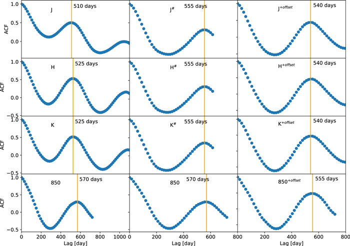
Figure B1. ACFs of J, H, K, and 850 μm passbands, from the entire data set we have (left), in a common time baseline with 850 μm (middle), and after the offset subtraction for the first period (right). The orange lines show the peak location which corresponds to the period obtained by the ACF. The peak locations are 510, 525, 525, and 570 days, respectively, when we use the whole data set. Using a common time baseline yields 555 days at the near-IR bands, and 570 days at the 850 μm band. After the offset subtraction 540, 540, 540, and 555 days, respectively, are obtained.
Download figure:
Standard image High-resolution imageWe identify the position of the second peak in each ACF as the period of the light curve. The uncertainty of the period is estimated at half of the sampling interval (7.5 days). Under the time window constraint but no offset (Figure B1, middle panel), the ACF periods show reasonable agreement across wavelengths, with periods of ≈550 days at all near-IR bands and ≈570 days in the submillimeter band. Applying the offset from Section 3.1 makes the agreement even better, 540 versus 555 days, respectively (Figure B1, right panel). For the unmodified, full near-IR data set, we find the ACF-determined periods are significantly shorter, 510–525 days (Figure B1, left panel). The results are presented in tabular form in Table 3.
Table 3. The Result of Period Determination
| Bands | LSP | ACF | LSPa | ACFa | LSPb | ACFb |
|---|---|---|---|---|---|---|
| J |
 , , 
|
510 ± 7.5 |

|
555 ± 7.5 |

|
540 ± 7.5 |
| H |
 , , 
|
525 ± 7.5 |

|
555 ± 7.5 |

|
540 ± 7.5 |
| K |
 , , 
|
525 ± 7.5 |

|
555 ± 7.5 |

|
540 ± 7.5 |
| 850 μm | ⋯ | ⋯ |

|
570 ± 7.5 |

|
555 ± 7.5 |
Notes.
aData points observed after JD = 2,457,421 are used. bData points obtained by UKIRT and the offset given before JD = 2,457,640.Download table as: ASCIITypeset image
B.2. LSP Analysis
We also apply an LSP (also called a least-squares spectral analysis; Lomb 1976; Scargle 1989) technique to the observed light curves to determine their periods using the LombScargle task in the timeseries package of astropy (Astropy Collaboration et al. 2013). The LSP is a powerful tool to detect periodic signals in discrete time-series data. The false-alarm probability (FAP) is calculated as described in Baluev (2008). For a detailed description, we refer the reader to VanderPlas & Ivezić (2015) and VanderPlas (2018). The best-fit periods along with the uncertainty in the period, determined through Gaussian fitting to each peak in the frequency domain, are tabulated in Table 3.
The LSP-determined periods are very similar to the ACF periods in all cases. For the full, unmodified near-IR data set an additional long-period signal, ≈4 yr, is found, along with the ≈500 day period (Figure B2, left panel). In a common time baseline with 850 μm but without the offset, this additional long-period component endures (Figure B2, middle panel). Applying the string length determined offset to the data prior to 2016 September 9 (Section 3.1), however, removes the long-term component and brings the determined periods, ≈540 days, into agreement with the submillimeter results, the ACF, and the string length method of Section 3.1 (Figure B2, right panel). We note that the FAPs of the peaks obtained by the LSP are well below the 10−6% level.
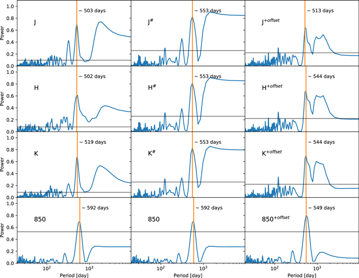
Figure B2. Periodograms of light curves in four different passbands—J, H, K, and 850 μm—from the entire data set we have (left), in a common time baseline with 850 μm (middle), and after the offset subtraction for the first period (right). The peak positions around 543 days are marked with orange vertical lines. The entire data set shows their peak at 503, 502, 519, and 592 days. The common time baseline with 850 μm shows 553, 553, 553, and 592 days. The step function applied light curves yield 513, 544, 544, and 549 days for the J, H, K, and 850 μm bands, respectively. The peaks appearing at ≈1700 days diminish after applying the step function. Gray solid horizontal lines indicate the power where the corresponding FAP is 10−3%.
Download figure:
Standard image High-resolution imageB.2.1. Periodogram Window Function
We obtain periodograms of the window function from the data set used for Appendix B.2 following Section 7.3.1 of VanderPlas (2018). As shown in Figure B3, there are notable peaks at ≈1 and ≈3 yr in the window function periodograms of the near-IR bands, reflecting the annual observing window for this source. For 850 μm, only minor peaks at 1 yr, ≈200 days, and ≈15 days appear. The 15 day peak corresponds to our observational cadence. None of the LSP-determined periods for EC 53 appears to be influenced by the window function.
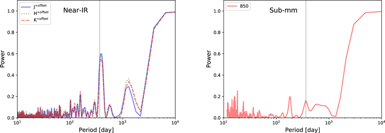
Figure B3. The window periodograms of the JHK (left) and 450 and 850 μm (right) bands. The gray solid line marks a 1 yr period.
Download figure:
Standard image High-resolution image