Abstract
The complex interplay of magnetohydrodynamics, gravity, and supersonic turbulence in the interstellar medium (ISM) introduces a non-Gaussian structure that can complicate a comparison between theory and observation. In this paper, we show that the wavelet scattering transform (WST), in combination with linear discriminant analysis (LDA), is sensitive to non-Gaussian structure in 2D ISM dust maps. WST-LDA classifies magnetohydrodynamic (MHD) turbulence simulations with up to a 97% true positive rate in our testbed of 8 simulations with varying sonic and Alfvénic Mach numbers. We present a side-by-side comparison with two other methods for non-Gaussian characterization, the reduced wavelet scattering transform (RWST) and the three-point correlation function (3PCF). We also demonstrate the 3D-WST-LDA, and apply it to the classification of density fields in position–position–velocity (PPV) space, where density correlations can be studied using velocity coherence as a proxy. WST-LDA is robust to common observational artifacts, such as striping and missing data, while also being sensitive enough to extract the net magnetic field direction for sub-Alfvénic turbulent density fields. We include a brief analysis of the effect of point-spread functions and image pixelization on 2D-WST-LDA applied to density fields, which informs the future goal of applying WST-LDA to 2D or 3D all-sky dust maps to extract hydrodynamic parameters of interest.
1. Introduction
Interstellar dust and gas indirectly trace ISM turbulence, rendering them a vital observational lever on the processes that shape star formation and galaxy evolution (Elmegreen & Scalo 2004; Goodman et al. 2009; Burkhart et al. 2015; Padoan et al. 2016; Krumholz et al. 2018). Furthermore, dust in the ISM produces a foreground signal that must be removed from extragalactic measurements, such as cosmic microwave background (CMB) temperature and polarization anisotropy (Planck Collaboration et al. 2017), and the spectra of galaxies, supernovae, and stars (Cardelli et al. 1989; Corasaniti 2006). However, the complex interplay of magnetohydrodynamics (MHD), gravity, and supersonic turbulence introduces non-Gaussian correlations into the density fields, complicating both the modeling of the dust, and its subtraction for cosmology (Kandel et al. 2017; Kritsuk et al. 2018).
A useful statistical starting point for describing (real and mock) ISM density fields is the two-point correlation function (2PCF), or its Fourier-domain analog, the Fourier power spectrum (PS) (Lazarian et al. 2001; Kowal et al. 2007). However, the 2PCF cannot describe non-Gaussian processes, because the power spectrum ignores phase information, which is important for higher-order correlations (Peek & Burkhart 2019). Higher-order correlation functions, such as the three-point correlation function (3PCF) and its Fourier-domain analog, the bispectrum, represent an improvement in terms of capturing higher-order correlations (Peebles 2001). The 3PCF has had significant success in the field of cosmology, describing the non-Gaussian distribution of galaxies (Slepian et al. 2017a, 2017b, and references therein). The 3PCF (Portillo et al. 2018) and bispectrum (Burkhart et al. 2009; Burkhart & Lazarian 2016) have also been applied to MHD simulations, and show some discriminatory power, but interpretation of these higher-order statistics remains difficult.
The wavelet scattering transform (WST) provides another way to go beyond the 2PCF and exhibits several convenient properties. It is an approximately translation-invariant image representation, which is linear (Lipschitz continuous) in its deformations (Bruna & Mallat 2012; Mallat 2012). This means that if an image is slightly deformed from i to  , the difference in the WST coefficients describing the two images is bounded by the size of the deformation. The success of the WST in image discrimination derives from its encoding non-Gaussianity (higher-order correlation functions), which allows the WST to distinguish images with the same Fourier power spectrum (see Figure 5 from Bruna & Mallat 2012). Furthermore, unlike explicit computation of the higher-order correlations, which is susceptible to large variance arising from outliers,
9
the WST coefficients are computed using non-expansive operators, and thus have lower variance.
10
The variance of the WST coefficients in response to outliers rapidly decreases as the maximum spatial scale size, J, increases,because outliers are suppressed via spatial averaging.
, the difference in the WST coefficients describing the two images is bounded by the size of the deformation. The success of the WST in image discrimination derives from its encoding non-Gaussianity (higher-order correlation functions), which allows the WST to distinguish images with the same Fourier power spectrum (see Figure 5 from Bruna & Mallat 2012). Furthermore, unlike explicit computation of the higher-order correlations, which is susceptible to large variance arising from outliers,
9
the WST coefficients are computed using non-expansive operators, and thus have lower variance.
10
The variance of the WST coefficients in response to outliers rapidly decreases as the maximum spatial scale size, J, increases,because outliers are suppressed via spatial averaging.
The WST performs well with regard to standard classification benchmarks (e.g., the MNIST digit data set, LeCun & Cortes 2010), even with minimal training data. It is sufficiently robust to temporal instabilities to characterize 1D time series data, such as the measured velocity at a point in turbulent gaseous flows (Bruna et al. 2015). Both 2D and 3D formulations of the WST have been applied to density functional theory (DFT) calculations of molecular structure (Hirn et al. 2017; Eickenberg et al. 2018). In addition, progress has been made in terms of image reconstruction based on WST coefficients, using generative networks (Angles & Mallat 2018), and gradient descent (Bruna & Mallat 2018).
The general class of wavelet techniques have long found applications in astrophysics. Early works analyzed 13CO velocity fluctuations in star-forming regions via wavelet transforms (Gill & Henriksen 1990). The wavelet transform modulus maxima (WTMM) approach was used to analyze ISM emission maps, including anisotropies in H i (Khalil et al. 2006) from the Canadian Galactic Plane Survey (Taylor et al. 2003), and non-Gaussianity (Robitaille et al. 2014) in the Herschel infrared Galactic Plane Survey (Hi-GAL) (Molinari et al. 2010). However, the WST is not merely a wavelet transform. It comprises repeated convolution by wavelets, and pooling under a nonlinear function (the modulus).
While originally introduced in the deep-learning community for image discrimination and classification, the wavelet scattering transform (WST) has recently made inroads in astrophysics. The WST has found applications in cosmology, in relation to state-of-the-art, large-scale structure syntheses, and cosmological parameter inference, where it outperforms the power spectrum in the context of weak lensing (Allys et al. 2020; Cheng et al. 2020). Recently, a reduced form of the WST (RWST) was introduced, to characterize the ISM with interpretable coefficients. The RWST was subsequently applied to Herschel observations and MHD simulations (in 2D) (Allys et al. 2019), as well as polarized dust emission (Regaldo-Saint Blancard et al. 2020).
The demonstrated capability of the WST to capture non-Gaussianity, its success in image classification problems, and prior applications to astrophysical data have motivated us to search for an optimal low-dimensional reduction of the WST for classification of dust density fields, in order to extract relevant hydrodynamic parameters. While convolutional neural nets (CNNs) have been trained to differentiate simulations that are sub/super-Alfvénic 11 (Peek & Burkhart 2019), as well as entire perpendicular velocity fields from MHD simulations (Asensio Ramos et al. 2017), we show that the WST provides “training-free” classification when combined with a fast and deterministic dimensional reduction step.
2. Methods
2.1. Non-Gaussian Descriptors
2.1.1. Three-point Correlation Function (3PCF)
For a given density field, I(
x
), correlations between three points, I(
x
1)I(
x
2)I(
x
3) for all
x
1,
x
2,
x
3, can be used to construct higher-order statistics that capture non-Gaussianity. We generally seek summary statistics that are translation-invariant, so we compute the translation and rotation-averaged product over three points, which yields the 3PCF. The 3PCF then depends only on three coordinates, which can be parameterized by r12, r13, and θ. Here, r12 is the distance from some base point,
x
1 to
x
2, r13 is the distance from
x
1 to
x
3, and θ is the angle between  and
and  . Correlations between
x
1,
x
2,
x
3 include contributions from the 2PCF between pairs of these three points (Groth & Peebles 1977). Setting the mean density to zero (i.e., ∫I(
x
)d
x
= 0) removes this dependence of the 3PCF on the 2PCF (see Appendix B). By expanding the angular dependence in terms of multipole moments around
x
1, this averaged-3PCF can be computed on a regular grid (of Ng points) with an FFT-based algorithm in
. Correlations between
x
1,
x
2,
x
3 include contributions from the 2PCF between pairs of these three points (Groth & Peebles 1977). Setting the mean density to zero (i.e., ∫I(
x
)d
x
= 0) removes this dependence of the 3PCF on the 2PCF (see Appendix B). By expanding the angular dependence in terms of multipole moments around
x
1, this averaged-3PCF can be computed on a regular grid (of Ng points) with an FFT-based algorithm in  time (Slepian & Eisenstein 2016). In 2D, we compute the projection of the 3PCF onto eimx
for m ≥ 0, where the coefficients for m < 0 are obtained by complex conjugation. Since the 3PCF is constructed as a triple product of a real field, the 3PCF must be real. However, our projection makes the 3PCF coefficients complex-valued in general. Viewing the Fourier expansion in terms of cosines and sines, where all coefficients are real, this is equivalent to saying that we find contributions which are anti-symmetric in θ. This is not possible in 3D, because a triangle defined by (r12, r13, θ) is equivalent to that defined by (r12, r13, -θ) under rotations and translations. However, in 2D, these triangles can only be identified under reflection.
12
Since previous works used only the even components of the 2D-3PCF coefficients (Zheng 2004; Chen & Szapudi 2005), we will provide comparisons using the real part of the coefficients in any case where we make use of the fully complex coefficients.
time (Slepian & Eisenstein 2016). In 2D, we compute the projection of the 3PCF onto eimx
for m ≥ 0, where the coefficients for m < 0 are obtained by complex conjugation. Since the 3PCF is constructed as a triple product of a real field, the 3PCF must be real. However, our projection makes the 3PCF coefficients complex-valued in general. Viewing the Fourier expansion in terms of cosines and sines, where all coefficients are real, this is equivalent to saying that we find contributions which are anti-symmetric in θ. This is not possible in 3D, because a triangle defined by (r12, r13, θ) is equivalent to that defined by (r12, r13, -θ) under rotations and translations. However, in 2D, these triangles can only be identified under reflection.
12
Since previous works used only the even components of the 2D-3PCF coefficients (Zheng 2004; Chen & Szapudi 2005), we will provide comparisons using the real part of the coefficients in any case where we make use of the fully complex coefficients.
We modified an unpublished 2D version of the code described in Portillo et al. (2018), and increased the speed. The code we used is publicly available (see Section 6). We characterize a 3PCF computation by the number of radial bins selected for r12 and r13, and the maximum multipole moment ( ) retained in the expansion. A 3PCF, with Nbins and a maximum multipole moment of
  , therefore has
  coefficients; the
  comes from multipoles running from
  , and the factor of 2 comes from the symmetry between r12 and r13. The 3PCF is averaged over the radii spanned by each bin. For optimal comparison to the WST, we have selected eight logarithmic radial bins, bounded by 2j
, for j = 0,..., 8.
13
, and the factor of 2 comes from the symmetry between r12 and r13. The 3PCF is averaged over the radii spanned by each bin. For optimal comparison to the WST, we have selected eight logarithmic radial bins, bounded by 2j
, for j = 0,..., 8.
13
2.1.2. 2D Wavelet Scattering Transform (2D-WST)
In 2D, a WST is specified by (J, L, M), where J is the maximum scale, L is the number of angular bins (i.e., the angular spacing is 180°/L), and M is the maximum order of the transform. The maximum scale and number of angular bins (J, L) define the set of Morlet wavelets ψj,l used in the transform. 14 The parent Morlet wavelet is the product of a plane wave of unit wavenumber with a Gaussian window of width σ. In one dimension, the wavelet is given by

where α and β are normalization factors (Ashmead 2010). We choose α so that the wavelets cover the Fourier domain as uniformly as possible. We choose β such that ψ has a null average.
In 2D and above, the inverse variance, 1/σ2, of the Gaussian window becomes an inverse covariance matrix. We choose a diagonal covariance matrix, with σyy = 2σxx (where x is the direction of the plane wave), to enhance the directionality of the wavelets. We choose σxx = 0.8 for our 2D-WST, which limits the number of oscillations of the plane wave, thereby enhancing filament identification. Each wavelet used in computing the WST coefficients is said to represent an oriented scale, indexed by (j, l) ∈ ([0, …, J − 1], [0, …, L − 1]), and is obtained from the parent wavelet by rotation and scaling of the argument (by 2j ) and frequency (by 2−j ). 15 While we use l as an index, we denote the corresponding angles as θ ∈ [π/2 − π/L,..., − (L − 1)π/2L, − π/2]. The wavelet, ψj,l , has a bandwidth of ∼2−j , and is centered at a wavevector of magnitude ∼2−j and angle θ, corresponding to l in the Fourier domain (Figure 1).
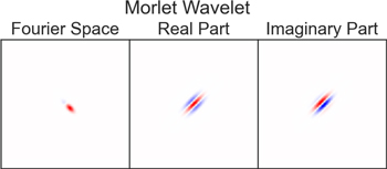
Figure 1. Confirmation of an example Morlet wavelet, ψj,l , with (j, l) = (3, 5) or (j,θ) = (3, − π/4), for a 2562 image in the Fourier domain (left). The real (middle) and imaginary (right) components of the wavelet are shown in the spatial domain. Angles are defined positive clockwise from north.
Download figure:
Standard image High-resolution imageThe WST can be represented as a convolutional network, with layers labeled m from 0 to M. We will outline the computation of coefficients for each layer for a network where M = 2. Coefficients for the mth layer are derived from m convolutions of the image field I( x ), with Morlet wavelets under the usual modulus for complex numbers. Normalization of the coefficients is relative to the response to a Dirac delta distribution, δ2D( x ):

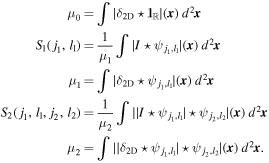
Here,  is the indicator function, which is 1 everywhere in the image. For μ0 and μ1, the convolution simplifies to the area of the image, and the sum of
  over the image, respectively.
16
Note that first-order coefficients depend on one oriented scale (j1, l1), while second-order coefficients depend on two oriented scales, (j1, l1) and (j2, l2). Since the first convolution obscures information at scales below
over the image, respectively.
16
Note that first-order coefficients depend on one oriented scale (j1, l1), while second-order coefficients depend on two oriented scales, (j1, l1) and (j2, l2). Since the first convolution obscures information at scales below  pixels, only coefficients with j2 > j1 are computed, such that one is then only looking at scales
  . We have one coefficient for m = 0, JL coefficients for m = 1, and J(J − 1)L2/2 coefficients for m = 2, for a total of J(J − 1)L2/2 + JL + 1. The WST coefficients at the mth layer depend on correlation functions up to order 2m
(proof in Mallat 2012). Thus, M > 1 is required to capture non-Gaussianity, because for m = 1, the WST coefficients depend predominantly on the 2PCF. For many applications, the spectral energy falls off rapidly with m; as such, M = 2 provides sufficient sensitivity to non-Gaussianity with a tractable number of coefficients.
. We have one coefficient for m = 0, JL coefficients for m = 1, and J(J − 1)L2/2 coefficients for m = 2, for a total of J(J − 1)L2/2 + JL + 1. The WST coefficients at the mth layer depend on correlation functions up to order 2m
(proof in Mallat 2012). Thus, M > 1 is required to capture non-Gaussianity, because for m = 1, the WST coefficients depend predominantly on the 2PCF. For many applications, the spectral energy falls off rapidly with m; as such, M = 2 provides sufficient sensitivity to non-Gaussianity with a tractable number of coefficients.
We normalize the 2D-WST coefficients following Allys et al. (2019), and Bruna et al. (2015), as

This normalization makes the first- and second-order coefficients invariant under multiplication of the field by a constant factor, and makes the second-order coefficients invariant to modification of the spectrum of the field by the action of a class of linear filters (Bruna & Mallat 2018).
2.1.3. 3D Wavelet Scattering Transform (3D-WST)
In 3D, the WST coefficients are defined similarly, except that solid harmonic wavelets (denoted by  ) are used in place of Morlet wavelets, with m ∈ [ − l,…,l − 1, l].

Here, Yl m are the Laplacian spherical harmonics, with (j, l) ∈ ([0,…,J − 1, J], [0, …, L − 1, L]). This corresponds to the choice of σ = 1 for the Gaussian window; the j-dependent wavelets are obtained by scaling the argument, as for 2D. We follow the implementation in kymatio 17 (Eickenberg et al. 2018), averaging over m in computing both the first- and second-order coefficients. For first-order coefficients, this is explicitly

where q = 1. For the 3D-WST, S2(j1, j2, l1) is a function of one angular scale only, we take l2 = l1. This means that the second-order coefficients are obtained between scales at the same angles only (rather than the Cartesian product of all angles). We compute the convolution coefficients for q = 1/2 and q = 2, in addition to q = 1, which is the exclusive power used in 2D-WST, although we comment only briefly on the q ≠ 1 cases. 18 There are (L + 1)(J + 1) coefficients for m = 1, and (L + 1)J(J + 1)/2 coefficients for m = 2, for a total of (L + 1)(J2 + 3J + 2)/2 (for each power q computed).
2.1.4. Reduced Wavelet Scattering Transform (RWST)
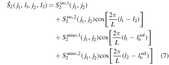
The RWST reduction (which is only defined in 2D) takes advantage of the periodicity observed in the WST coefficients to remove the angular dependence (see Appendix C). Explicitly, the RWST coefficients are obtained from the WST coefficients by a least-squares fit of the first- and second-order coefficients. For the first order,

where  ,
,  , and
, and  are fit coefficients. For the second order,
where  ,
,  ,
,  ,
,  , and
, and  are fit coefficients. There are 3J coefficients for m = 1, and 5J(J − 1)/2 coefficients for m = 2, for a total of J(5J + 1)/2.
19
are fit coefficients. There are 3J coefficients for m = 1, and 5J(J − 1)/2 coefficients for m = 2, for a total of J(5J + 1)/2.
19
2.2. Dimensional Reduction Algorithms
In order to interpret these high-dimensional (>100 coefficients), non-Gaussian descriptors, we employ dimensional reduction techniques, including principal component analysis (PCA), linear discriminant analysis (LDA), and quadratic discriminant analysis (QDA). 20 PCA is an unsupervised technique, in which the ith principal component is orthogonal to the first i − 1 principal components, and is in the direction of maximal remaining variance (Jolliffe & Cadima 2016). In contrast, LDA and QDA are supervised techniques, meaning that they take class labels (here, hydrodynamic parameters) in addition to the high-dimensional descriptor of a data point (here, the WST, RWST, or 3PCF coefficients). LDA assumes that each component of the high-dimensional descriptor is normally distributed, and that all classes share the same covariance matrix; this latter assumption is known as homoscedasticity (Bandos et al. 2009). LDA then finds the hyperplanes that best separate the K classes in the K − 1 dimensional space containing the class means. The hyperplanes are found using eigenvalue decomposition, involving the inter- and intra-class scatter matrices. This is equivalent to evaluating the Gaussian likelihood that each input is in each class, and assigning the input to the class with the greatest likelihood. Note that the LDA components (which maximize the separation between classes) need not be orthogonal. The LDA components are in units of σii , the on-diagonal components of the shared covariance matrix. QDA is similar to LDA, except that it drops the assumption that the covariance matrix must be the same for all classes, and thus finds conic sections that best separate the classes, rather than hyperplanes. The boundary between two neighboring classes occurs where the Gaussian likelihoods of each class are equal, which is in general a quadratic function (as in QDA), but simplifies to a linear function when the class covariances are assumed equal (as in LDA).
3. Data Sets
In this section, we introduce the observational data sets and MHD simulations used to verify the sensitivity of our method to non-Gaussianity and test its capabilities in terms of the classification of turbulence.
3.1. SFD Dust Map
Interstellar dust is an indirect tracer of interstellar turbulence, and provides an observational point of comparison to the MHD simulations discussed below. Dust grains are heated to ∼20K by ambient starlight, and produce thermal emissions in the far-infrared (Low et al. 1984). We use the SFD dust map (Schlegel et al. 1998), which is based on this thermal emission. The map derives dust morphology from 100 μm data from the Infrared Astronomical Satellite (IRAS) Sky Survey Atlas (Neugebauer et al. 1984; Wheelock et al. 1994), corrected for temperature variation using data from the Diffuse InfraRed Background Experiment (DIRBE) on the Cosmic Background Explorer (COBE) (Mather 1982; Boggess et al. 1992).
To obtain a representative sample of 2D dust images, we reproject the SFD dust map with bilinear interpolation to a TAN (gnomonic) projection, centered on random locations on the celestial sphere. Each 2562 pixel image has a random position angle, a pixel scale of 30, and a point-spread function (PSF) full width at half maximum (FWHM) of 6
1. The SFD bitmask flags regions with missing IRAS data (bit 128), pixels in the Magellanic clouds or M31 (bit 64), and regions with no point-source subtraction (mostly at low Galactic latitude, ∣b∣ < 5°; bit 32). An image is discarded if any pixel has any of these mask bits set, leaving a sample of 10,222 images (Figure 2).
21
By rejecting images near the Galactic plane, we focus on the morphology of relatively nearby dust (on the order a few 100 pc to a few kpc), where each image is dominated by dust at one, or a few, distances. The statistics of the dust distribution near b = 0 might be substantially different, owing to the large number of clouds along each line of sight, and the steep dependence on latitude. The images are normalized to have [min,max] = [0,1] for input to the WST, and zero mean with unit variance for input to the 3PCF, consistent with other images used in the paper.
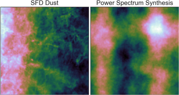
Figure 2. Left: representative 2562 image of the 2D SFD dust map (log color scale). Right: same as left, but with random phase in the Fourier domain (linear color scale). High intensity (light colors) corresponds to large amounts of extinction, and hence high dust density, while low intensity (dark colors) corresponds to low dust density. A log color scale is used only for the SFD image, so as to emphasize filament-like structures present in SFD, but not present in the power-spectrum synthesis. The relevance of phase coherence for the non-Gaussian filamentary structure is apparent by comparison. Units are obscured due to the [min, max] = [0, 1] normalization adopted here.
Download figure:
Standard image High-resolution image3.2. Magnetohydrodynamic Simulations
We use MHD simulations of turbulent gas flows published in previous works (Cho & Lazarian 2003; Burkhart et al. 2009; Portillo et al. 2018; Bialy & Burkhart 2020; Burkhart et al. 2020), and review only key properties. The simulations solve the ideal MHD equations constraining the divergence to zero (∇ · B = 0), assuming an isothermal equation of state, and periodic boundary conditions. No gravity is included, and the simulations are “scale-free.” The simulation box measures 2563 voxels, and is driven isotropically by random, divergence-free forcing, with wavenumber k ≈ 2.5 (i.e., 1/2.5 the box size). No dissipation is assumed, other than numerical dissipation from the finite resolution of the simulation. The magnetic field is initialized uniformly in the x-direction.
Each simulation is characterized by its Alfvénic Mach number (MA), and sonic Mach number (MS). The Alfvénic Mach number is defined as MA ≡ ∣v∣/〈vA〉, where v is the flow velocity, and 〈vA〉 the Alfvén (magnetic wave) speed averaged over the simulation box. The sonic Mach number is defined as MS ≡ ∣v∣/cs , where cs is the isothermal speed of sound. We use MA = 0.7, 2.0, and MS = 0.7, 1.0, 2.0, 4.0 to include sub-Alfvénic (MA = 0.7) and super-Alfvénic (MA = 2.0) cases, as well as subsonic (MS = 0.7), transonic (MS = 1.0), and supersonic (MS = 2.0, 4.0) cases (Figure 3). The images are normalized to have [min,max] = [0,1] for compatibility with the log normalization of the WST, but we have confirmed that our WST classification result is reproduced if one uses zero mean and unit variance normalization. The images are normalized to have zero mean and unit variance when computing the 3PCF, in order to exclude any contributions from the 2PCF (see Appendix B).
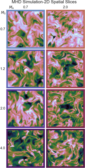
Figure 3. Representative 2562 slices of the density field for MHD simulations at various Alfvénic (MA) and sonic Mach numbers (MS). The image axes are spatial coordinates at a fixed value for the third spatial coordinate of the simulation box. Density units are obscured by the [min, max] = [0, 1] normalization adopted here. High intensity (light colors) corresponds to high density, and low intensity (dark colors) corresponds to low density. A log color scale is used to emphasize density variance across spatial scales. Plotted on the same scale, larger sonic Mach numbers show larger density fluctuations, but this information is rescaled by normalization prior to computing the relevant statistic.
Download figure:
Standard image High-resolution image4. Results and Discussion
We begin by comparing the performance of the WST, RWST, and 3PCF in capturing non-Gaussianity. We then combine these statistics with LDA to classify turbulent MHD simulations, and investigate the robustness of WST-LDA in relation to modifications of the sample images.
4.1. Sensitivity to Non-Gaussianity
We assess the performance of the WST, its reduction the RWST, and the 3PCF as high-dimensional descriptors for the characterization of non-Gaussianity in 2D images. Each of these descriptors is then used in conjunction with two dimension-reduction techniques, PCA, and LDA. PCA and LDA are used to probe the information contained in the high-dimensional parameter spaces, corresponding to the WST, RWST, and 3PCF coefficients. We begin by confirming that these descriptors are sensitive to non-Gaussianity by applying them to 2D dust map images. We compute the WST coefficients (J = 8, L = 8, M = 2) on 10,222 SFD images (“SFD”), 22 2000 images where each pixel is a uniformly drawn pseudo-random number [0,1) (“Rand”), and those same random images, convolved with a σ = 4 pixel uniform Gaussian (“Smooth”). This latter set imposes nearest-neighbor correlations, which are present in empirical images due to the continuity of real density fields and instrumental point-spread functions. To further prove that the WST captures non-Gaussianity, we compute the WST coefficients for images where the Fourier power spectra matches the SFD images, but with small higher-order correlations (“NHC”). Specifically, for each image in the SFD set, we apodize the image (i.e., multiply by a generalized Gaussian, 23 p = 6, σ = 100), compute the Fourier transform (FT), randomize the phase (with a unique pseudo-random seed), and compute the inverse FT. 24 The RWST and 3PCF (Nbins, L) = (8, 9) coefficients are also computed on the same four data sets for comparison.
To investigate the variance of these coefficients with respect to prototypical 2D dust, we perform PCA 25 on the coefficients from the SFD set and then project the results from the other three control image sets (“Rand,” “Smooth,” “NHC”) onto those principal components. Each point in Figure 4 corresponds to an image from one of the data sets above.
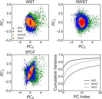
Figure 4. Individual image representations in the first two SFD principal components (PCs) are shown for “SFD” (green), “NHC” (blue), “Smooth” (yellow), and “Rand” (red). We define these PCs for the WST (top left), RWST (top right), and 3PCF (bottom left) coefficient representations for each image. PC axes are reported in units of the standard deviation of that PC. The bottom right panel shows the cumulative variance of the “SFD” set, explained by the first N principal components (PC) for each statistic. We see the cumulative variance saturate at around 5–10 PCs, implying that not many principal components are required to capture the majority of the variance. An interactive version of this figure is available at https://faun.rc.fas.harvard.edu/saydjari/RWST_2020/SFD_PCAs.html, showing partial separation of the four classes when the inputs to PCA are not scaled to have zero mean and unit variance.
Download figure:
Standard image High-resolution imageIn WST-PCA space, the SFD data set presents as an ellipsoid, with a population of outliers extending along the first PC axis in the positive direction. The “NHC,” “Smooth,” and “Rand” data sets present as progressively narrower ellipsoids overlapping the main mass of “SFD.” While slight, the different orientation of these ellipsoids may encode more detailed information differentiating the data sets. We observe that, to first order, the diameter of the ellipsoids decreases with the progressively decreasing pixel – pixel correlations in the “SFD” > “NHC” > “Smooth” > “Rand” series. This suggests that the variance in the WST coefficients on “SFD” images primarily arises from higher-order correlations, as desired. As shown in the cumulative variance plot, most of the variance of “SFD” is described by the first few PCA components, suggesting that WST-PCA admits a low-dimensional representation of SFD dust. By cross-referencing the Galactic coordinates of the images associated with the outliers in the “SFD” data set, using glue, 26 we associated most of the outliers with images of the Orion nebula. The formation of massive stars in the Orion nebula modifies the dust distribution, and is likely to give rise to outliers in the WST-PCA space. This was also true for the outliers in the RWST-PCA and 3PCF-PCA bases. The sensitivity of WST-PCA to outliers may suggest its potential application in the area of outlier detection and flagging in large survey pipelines.
When the input coefficients to PCA are not scaled, the mean and variance of the WST coefficients are sufficient to partially separate all four data sets in WST-PCA space (see the interactive version of Figure 4). This is in contrast to what is expected for a simple N-point correlation function, which should have an expectation value of zero for N > 2 on “NHC,” “Smooth,” and “Rand.” While exclusion of the S0 coefficient does not visibly inhibit class separation, we cannot rule out that information regarding the mean of the density distribution does enter the higher-order coefficients, owing to the [min,max] = [0,1] normalization we chose. We therefore believe that a more careful study of the distribution and expectation values for the WST coefficients is called for in future work.
The distributions of the four data sets under RWST-PCA are similar to the distribution under WST-PCA, except that the ellipsoidal distributions have lower eccentricity. The unscaled RWST-PCA basis also partially separated the four classes, and further improved the separation of “Rand” to have no overlap with the other three classes. The cumulative variance rises much more slowly as a function of the number of principal components, suggesting that the RWST does not admit as low-dimensional a representation, and that the variance in “SFD” under the RWST is similar for many directions.
We select the real part of the 3PCF coefficients for analysis by PCA. The distribution of the four data sets under 3PCF-PCA is similar to that under WST-PCA, except that “Smooth” and “Rand” have higher and lower eccentricities, respectively. The unscaled 3PCF-PCA basis separates “SFD” from the other three data sets, with little overlap. However, the expectation value of the 3PCF for “NHC,” “Smooth,” and “Rand” must be zero. As such, the centroids for all three data sets are coincident. Despite overlapping centroids, the major axes of “NHC” and “Smooth” are distinct, allowing partial separation. The distribution of “Rand” is so tight and circular that it overlaps entirely with “NHC” and “Smooth.” The cumulative variance of the 3PCF is between that of the WST and RWST, suggesting the 3PCF admits an intermediate-dimensional representation of SFD dust. We repeated this analysis, taking the modulus of the 3PCF coefficients instead. While the exact shape of the distribution for each data set changed, and the centroid of “NHC,” “Smooth,” and “Rand” shifted, the separation was not strongly affected. 27
The lack of complete separation in the PC basis does not mean that these descriptors do not contain the information necessary to distinguish the four classes. PCA is an unsupervised technique, and as such cannot optimize for the separation of classes, as it has no knowledge of them. To determine whether the computed coefficients can distinguish the four classes, we turn to a supervised learning technique, LDA. We split the data sets into test/train sets (80%/20%) and compute the confusion matrix for the test set between the true labels and the assignment predicted by the LDA model, which was trained on the first set. 28 In the confusion matrix, we show the actual number of images having a true class label that were predicted to have a certain class label. The grayscale coloring of the matrix indicates the true positive percentage relative to the number of test images, with the corresponding true label (the row sum). In this way, the row sum is always the test fraction (∼0.2) times the total number of images in each class. To quantify the predictive power of LDA on this multi-class problem, we report the precision score, which is the total fraction of correctly classified images (true positive percentage).
Figure 5 illustrates that the WST contains enough information to completely distinguish the four classes, and can thus at least partially characterize the non-Gaussianity of SFD dust. The RWST performs similarly well, apart from the presence of an outlier in the RWST-LDA space that is not associated with any of the clusters. These outliers tend to result from undertraining, i.e., failing to fully constrain non-discriminatory dimensions. While not shown, we also analyzed an RWST model, where the frequency in Equations (6) and (7) were fit in addition to the usual RWST parameters. This unfortunately created a large degeneracy between the reference angle and frequency, which caused fitting instability and massive variability that were common to all data sets (not discriminatory). Outliers may also arise when the cosinusoidal dependence is so small in amplitude that the angle is undefined, or when the cosinusoidal frequency differs from the model. These points demonstrate that more work remains to be done to regularize the RWST technique.
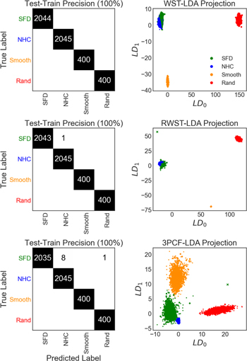
Figure 5. Confusion matrix between “SFD,” “NHC,” “Smooth,” and “Rand” when applying WST-LDA (top left), RWST-LDA (middle left), and 3PCF-LDA (bottom left). Matrix entries are the number of test images with the corresponding true-predicted label pairing. The grayscale color indicates the true positive percentage, relative to the number of test images with the corresponding true label. Test images are shown in the first two components of LDA space for the WST (top right), RWST (middle right), and 3PCF (bottom right). Circle markers represent images that were correctly assigned, and cross markers represent those incorrectly assigned. In all cases, colors correspond to true labels. An interactive version of this figure is available at https://faun.rc.fas.harvard.edu/saydjari/RWST_2020/SFD_LDA.html, and shows the images in LDA space, and, allowing for isolation of the train, correctly labeled test images, and incorrectly labeled test images.
Download figure:
Standard image High-resolution imageFor improved classification, we take the modulus of the 3PCF coefficients as inputs to LDA. Under these conditions, 3PCF-LDA almost completely distinguishes the four classes, with only a few images of “SFD” confused for “NHC”, and one extreme outlier. Viewed in the interactive version of Figure 5, these confused images between “NHC” and “SFD” are associated with the “SFD” cluster, suggesting that the misclassification derives from the strictly linear boundaries to which LDA is limited. In addition, the assumption of equal class covariances (homoscedasticity) is strongly violated for the 3PCF, because the variance is strongly class-dependent (Figure 5, bottom right). To attempt to further improve classification with 3PCF, we use QDA, which relaxes the homoscedasticity condition, and removes the confusion between “NHC” and “SFD.” In all other sections of the manuscript, LDA and QDA produce nearly identical results, and so only the simpler LDA results are presented. When attempting classification with only the real part of the 3PCF coefficients, there was a large confusion between “NHC,” “Smooth,” and “Rand,” 29 which are forced to have exactly overlapping centroids. This condition is lifted upon taking the modulus, since the expectation value of the modulus of the 3PCF coefficients need not be zero on images drawn from Gaussian distributions.
In summary, all three non-Gaussian descriptors contain enough information to distinguish “SFD,” “NHC,” “Smooth,” and “Rand,” but with the WST, the classes can be distinguished using a simple linear classifier (in contrast to classification with the 3PCF), and without outliers (in contrast to classification with the RWST).
4.2. Classification of MHD Simulations
Since WST, RWST, and 3PCF distinguish Gaussian from non-Gaussian fields, we seek to use them to classify different physical processes that can contribute to non-Gaussianity. One application with implications for the ISM is inferring characteristic MHD parameters, such as the sonic and Alfvénic Mach number. We demonstrate the ability of WST-LDA to do this on idealized MHD simulations (Figure 3), as a proof of concept. For each of the eight conditions (sonic/Alfvénic Mach number pairs) we have the full density cube (2563 pixels) at nine time steps. Because the separation between these time steps is longer than the eddy turnover time, each can be treated as an independent sample for the given condition. For each cube, we take 2D slices (2562 pixels) along each axis (x, y, z), spaced every eight pixels so as to reduce the sampling redundancy. 30 Therefore, we computed the WST coefficients for 6,912 (8 × 9 × 32 × 3) images, or 864 images per class. To ensure that the test set is not correlated with the training set, all images in the test set are selected from two independent time steps, withheld from the training set. Since each time step is an independent sample, the test and train sets are thus independent.
We achieve a precision of 97% for WST-LDA (J = 8, L = 8, M = 2; Ncoeff = 1, 857), 98% for RWST-LDA (Ncoeff = 164), and 87% for 3PCF-LDA (Nbins = 8, L = 9; Ncoeff = 360) (Figure 6). The precision for WST-LDA is comparable to that obtained previously for differentiating sub/super-Alfvénic simulations after training a neural net (Peek & Burkhart 2019), but notably required no training except for a deterministic LDA step. As shown in the interactive version of Figure 6, the first three LDA components separate each of the classes. There is a small amount of crosstalk between adjacent classes, due to scatter of the WST coefficients of images in the same class.
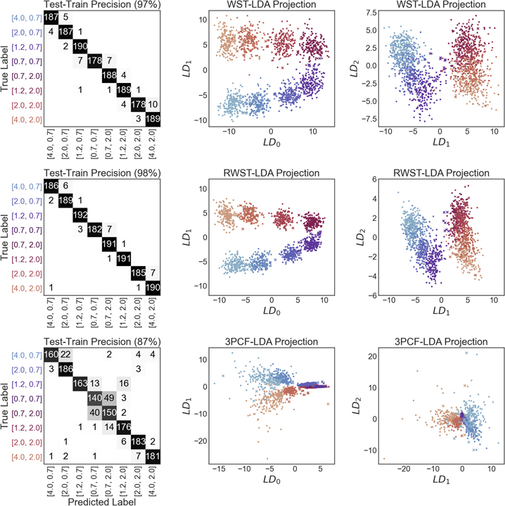
Figure 6. Confusion matrix between MHD classes labeled by [sonic, Alfvénic] Mach numbers, when applying WST-LDA (top left), RWST-LDA (middle left), and 3PCF-LDA (bottom left). Matrix entries are the number of test images with the corresponding true-predicted label pairing. The grayscale color indicates the true positive percentage relative to the number of test images with the corresponding true label. In all cases, colors correspond to true labels, as indicated on the vertical axis in the left panels. Test images are shown in the first two components of LDA space for the WST (top right), RWST (middle right), and 3PCF (bottom right). Circle markers represent images that were correctly assigned, and cross markers represent those incorrectly assigned. The RWST outlier in (4.0, 2.0) classified as (4.0, 0.7) is far outside the axes limits. An interactive version of this figure is available at https://faun.rc.fas.harvard.edu/saydjari/RWST_2020/MHD_LDA.html, showing the images in LDA space, and allowing isolation of the train, correctly labeled test images, and incorrectly labeled test images. The WST, RWST, and 3PCF in combination with LDA all classify the MHD simulations with high precision, although we prefer the linear spacing of classes in the (R)WST-LDA basis.
Download figure:
Standard image High-resolution imageSince these MHD parameters are actually continuous variables, the variance of each class can be viewed as an indicator of the uncertainty of an inference of these MHD parameters from a single image. To obtain a rough estimate of this uncertainty, we assume MS varies linearly as a function of separation between clusters of the same MA value. Then, we find that MS only varies ∼10% within 1σ of the centroid of each cluster. Thus, for these simulations, we can approximately infer MS ± 10%. Note that the sonic Mach numbers studied here are lower than the average estimated for molecular clouds in the ISM from CO line widths (∼10–20, Kainulainen & Tan 2013; Kainulainen & Federrath 2017), but comparable to measurements for 21-cm cold neutral medium (CNM) (Heiles & Troland 2003; Burkhart et al. 2010). However, whether this approximately linear mapping of MS to LDA space holds at larger MS remains an open question. We hold off on a comparison between observations and simulations until we can characterize a wider range of Mach numbers and other physical parameters.
In this WST-LDA space, the classes of images with different Alfvénic Mach number form a helical structure (Figure 3, interactive version). Along the vertical axis of the helix, the sonic Mach number varies monotonically while the separation in the plane perpendicular to this axis determines the Alfvénic Mach number. We can also see this behavior in the 2D projections, where LD0 is the helical axis (Figure 6). There is little structure as a function of Mach numbers in the 4th and higher LDA components, suggesting the classification occurs primarily in a 3D subspace of the WST-LDA basis.
The increased precision of RWST-LDA as compared to WST-LDA appears to derive from reduced scatter around the centroids of each cluster, although the centroids are separated by the same distance. Since LDA selects the optimal linear combination of the WST coefficients, the success of RWST is not simply in selecting an optimal subset of the coefficients containing the most information; the RWST is not simply performing dimensional reduction. The nonlinear combination of WST coefficients used by the RWST preferentially selects information relevant to differentiating the MHD classes.
For improved classification, we take the modulus of the 3PCF coefficients as inputs to LDA, and find partial separation of the classes. We find that the variance is strongly class-dependent, with higher sonic Mach numbers having larger variance, and lower sonic Mach numbers having smaller variance. This suggests that the variance of the 3PCF is sensitive to sharp density fluctuations. Furthermore, the spacing of the centroids is highly nonlinear. The small spacing between these centroids for MS = 0.7 is the source of most of the confused images. 31 This small spacing suggests the contribution of an important influence from MA in the fourth-order moments, which is present in the WST, but not in the 3PCF. As aforementioned, for cold gas in the ISM, MS is likely to be >0.7; as such, this lack of discriminatory power for low MS may not be a problem for some applications. The fact that gas near young hot stars has lower MS suggests that it may be more difficult to apply WST-LDA to active star-forming regions (Gallegos-Garcia et al. 2020).
Since dust maps such as SFD project a 3D volume along the line of sight down to 2D, we investigate how WST-LDA, RWST-LDA, and 3PCF-LDA perform with respect to projected images by repeating our sampling procedure on the cumulative sum of density along a given coordinate axis. This is equivalent to sampling the column density along the line of sight in the optically thin limit. We computed the WST coefficients for the same number of images as before, i.e., 6912. Note that the line of sight sums introduce further correlations, thereby reducing the effective size of our data set, and can be seen as clusters or lines within a given class. We find a precision of 57% for WST-LDA, 83% for RWST-LDA, and 44% for 3PCF-LDA (see Appendix D, and the figure therein). The improvement provided by the nonlinear transforms in the RWST becomes even clearer in the context of cumulative sums, and we anticipate that this will be instrumental in applications featuring multiple clouds along the line of sight.
Overall, the WST and RWST seem most suited to the continuous inference problem of estimating Mach numbers from measured density fields, since MS maps approximately linearly into the LDA classification space, in contrast to the highly nonlinear mapping for 3PCF-LDA. While the nonlinear transformations of WST coefficients made by the RWST improve the classification, as well as rendering the classification more robust to cumulative sums, future work should seek an optimal nonlinear transformation of WST coefficients that does not also create outliers. Since we do not yet have such an optimal transformation, we focus here on characterizing the performance of WST-LDA on several test cases.
4.3. 2D/3D Scale Dependence of WST-LDA
It is important to establish how many coefficients the WST needs to characterize a non-Gaussian process. However, this question is intertwined with that of the scale at which the process of interest is occurring, and how many different scales the WST needs to characterize a non-Gaussian process. We study this trade-off in our MHD test case by computing those scattering coefficients that include only a subset of the scales in the problem. Firstly, we compute the WST coefficients for L = 8, M = 2, and J = 3, 4, 5, 6, 7, and 8 to investigate the effect of the maximum scale ( ).
32
We can follow a similar process to find
).
32
We can follow a similar process to find  by subsampling the 2562 image down to a
  image (i.e., binning down by a factor of
  ), and computing the WST with L = 8, M = 2, and J = 8, 7, 6, 5, 4, and 3. Both results are shown in Figure 7. Note that the
  (var) and
  (var) curves cross at j = 4. The j = 0 (smallest spatial) scale is likely to contain little information if the image is well sampled. Above the j = 0 scale, the linearity of each of the data sets suggests that there is approximately the same information content in each scale.
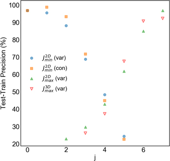
Figure 7. Scale-dependent classification precision for WST-LDA on MHD simulations. “ (var)” (blue, circle) was obtained using a smaller-J WST after resampling images. “
 (var)” (green, triangle) was obtained by computing the WST on a
  subset of the original images. “
 (con)” (orange, square) was obtained by computing the WST for J = 8 on images which were downsampled to 2562 after repeated tiling of the image.
  (variable) (red, inverted triangle) was obtained by computing the WST on a
  subset of the original volumes. Since
  “constant” is always within 6% of
  “variable,” we conclude that the trend observed in
  “variable” is predominantly the result of the scales excluded, and not due to the number of coefficients.
Download figure:
Standard image High-resolution imageThe number of coefficients (the dimension of the WST vector) decreases as we narrow the range of scales in the above analysis. To test whether the loss of information results explicitly from reduction in the number of coefficients versus loss of information in the image due to binning effectively eliminating certain scales, we generate a series of images of fixed size but with increasing redundancy. We leverage the fact that these simulations have periodic boundary conditions, and can therefore repeat a given image in a 2n
× 2n
matrix, downsample the image to 256 × 256 resolution, and always compute the WST for J = 8, L = 8, M = 2. These results ( “constant”) are always within 6% of the
  “variable”, so we conclude that the trend observed in the
  “variable” is predominantly the result of the scales excluded, and is not due the number of coefficients.
While the highest-resolution maps of the ISM are 2D, the resolution of 3D maps is improving (Green et al. 2019; Leike et al. 2020). Owing to the fact that the physical processes driving the structure of the ISM are happening in 3D, one may expect a measurement of non-Gaussianity that is computed in 3D to capture more information. We show that 3D-WST-LDA (J = 6, L = 8, M = 2) is comparable to 2D-WST-LDA in terms of separating the eight classes in our set of MHD simulations when the same scales are included (Figure 7). 33 3D-WST-LDA specifically outperforms 2D-WST-LDA by ∼5% for j = 5, 6. Note that 3D-WST is a strictly lower dimensional representation for all j studied, as we do not compute second-order coefficients between different angular bins in the 3D-WST procedure. 34 2D-WST and 3D-WST also use different wavelets (see Equations (1) and (4)) and so we leave a more detailed comparison of the different bases to future work. 3D-WST-LDA can clearly provide similar classifications to 2D-WST-LDA, though the increased computational expense means it is only likely to be used when 3D correlations are necessary (see Appendix A for computational costs).
4.4. Robustness of Classification
4.4.1. Using Velocity Information
While few 3D maps of the ISM exist in position–position–position (PPP) space, and those that do exist are of relatively low resolution (1 pc; Leike et al. 2020), high-resolution maps of gas tracers (H i, 12CO, 13CO) in position–position–radial velocity (PPV) space are available (Dame et al. 2001; Ridge et al. 2006; Pineda et al. 2008; Peek et al. 2018; Clark & Hensley 2019). These PPV maps are also used to constrain the sonic Mach numbers of molecular and atomic clouds (Heiles & Troland 2003; Burkhart et al. 2010; Kainulainen & Tan 2013). We convert our MHD simulations to PPV space by interpolation, using the density field and x-velocity field. 35 Representative 2D slices in PP and PV space are shown in Figure 8. Classification of 2D slices was difficult (average precision 63%), but by utilizing the 3D-WST (J = 6, L = 8, M = 2), we achieved a precision of 71%. 36 We suspect that the reason for the difficulty in terms of 2D classification is that there is little correlation between the density and velocity fields observed by Burkhart et al. (2009). However, those authors noted a correlation between Mach numbers and velocity dispersion, which may explain why the 3D-WST in PPV space, which captures a large range of velocities, performs well. The spherical harmonic-based wavelets used here treat all three axes identically. While the velocity axis is not interchangeable with the two position axes, we use these simple wavelets to demonstrate the benefit of the correlation between velocity and position channels. 37 This ability of WST-LDA to operate in PPV space has potential application both to a wider variety of data, and to higher-resolution 3D data. This higher-resolution PPV data may prove invaluable for mapping regions with overlapping clouds observed in dust and gas tracers. Given that a large range of velocities was required to determine the Mach number, resolving overlapping clouds may be difficult, unless the clouds are well-separated in velocity space.
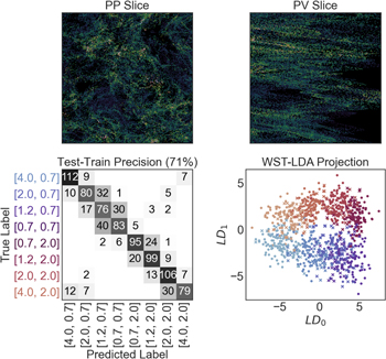
Figure 8. Representative position–position (PP) slice for fixed velocity (top left) and representative position–velocity (PV) slice (top right). Both were plotted using a power-law color scale (γ = +0.4) to emphasize low density features. Bottom left: confusion matrix between MHD classes (labeled with [sonic, Alfvénic] Mach numbers) for the 3D-WST-LDA, where J = 6, L = 8, and M = 2. Matrix entries are the number of test voxels with the corresponding true-predicted label pairing. The grayscale color indicates the percentage of test voxels with the corresponding true label in the test set. In all cases, colors correspond to true labels, as indicated on the vertical axis in the bottom left panel. Bottom right: test and train voxels are plotted in the first two components of LDA space. Circular markers represent test voxels, and cross markers represent test voxels that were incorrectly assigned. Slices were taken from an MHD simulation in the (MA, MS) = (4, 2) class.
Download figure:
Standard image High-resolution image4.4.2. Artifacts and Missing Data
Pattern noise is a common feature in imaging data sets. Long-term sensitivity drift in scanning detectors produced stripe artifacts in IRAS (Wheelock et al. 1994) and AKARI (Doi et al. 2015). A ground loop in the readout electronics of a charge-coupled device (CCD) can imprint nearby radio transmissions on the data. 38 Even highly sophisticated instruments on the Hubble Space Telescope can experience electronics problems that leave subtle “herringbone” patterns in the data (Jansen et al. 2010). A desideratum of a classifier is that it be robust to such pattern noise, or at least be able to give warning of its presence.
For testing purposes, we mimic pattern noise by adding a sinusoidal pattern with a random wavevector to the MHD slices. Specifically, we generate for each MHD slice (6,912 draws) a random amplitude (10%–30% of signal max), phase, period width (2–25 pixels), and angle relative to the x and y axis, and add it to the MHD slice prior to computing the WST coefficients (Figure 9). In some cases, large contiguous regions of an image may be lost due to satellite transits, diffraction spikes, or ghosts of bright stars. We model this by introducing a cutoff for eliminating pixels, based on the sinusoidal field used above (in this case with periods in the range of 43-256 pixels, and amplitudes of 10%–20%). The sinusoidal field was not added to the data, but the values in the image were set to zero for all indices where the sinusoidal field exceeded 10% (Figure 9). In both cases, we observe at most a slight reduction in precision (96% and 94%, respectively, compared to 97%) and increased variance for each class. However, the quantitative classification is evidently robust to these artifacts, and the qualitative structure of the clusters in the space of the first three LDA components was also unaffected.
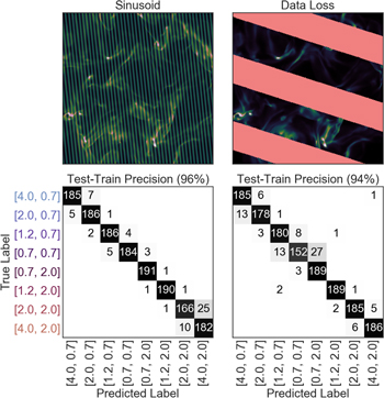
Figure 9. Example of additive sinusoidal noise (top left) and our data elimination scheme (top right). Removed data was set to light red on our color scale, for illustration purposes, but was set to zero when computing WST-LDA. Representative slices were taken from an MHD simulation in the (MA, MS) = (4, 2) class. Bottom: confusion matrix between MHD classes (labeled with [sonic, Alfvénic] Mach numbers) for the above noise models. Matrix entries are the number of test images with the corresponding true-predicted label pairing. The grayscale color indicates the percentage of test images with the corresponding true label in the test set. In all cases, colors correspond to true labels, as indicated on the vertical axis in the bottom left panel. In both cases, quantitative classification is evidently robust to these artifacts, because the precision is comparable to the noise-free value of 97%.
Download figure:
Standard image High-resolution image4.4.3. Dependence on Point-spread Function
In observational images, the true signal is also convolved with a point-spread function (PSF). We model this as a Gaussian PSF, with a FWHM of 2.355σ (in pixels). Moreover, we do not assume that the PSF is rotationally symmetric, and allow for nonzero aspect ratios AR = σx /σy . We investigated the following PSFs in detail: (σ, AR) = (2,1), (2,2), (4,1), (4,2), (4,3). The MHD classification by WST-LDA for samples from a single PSF was qualitatively unchanged, with a precision of ≥94%. Further, when all the WST coefficients from the PSF-blurred images and original images were combined, LDA was able to classify the images on Mach numbers with a precision of 92%.
However, we must emphasize that the optimal LDA space for each individual PSF is different. For instance, the LDA space for (2,1), and the LDA space for the original images are not the same. In the interactive version of Figure 10, we demonstrate how the WST coefficients for (2,1) look in the LDA space for the original images, and vice versa. While these spaces are not identical, the helix that we observed in the native LDA space is still present, but shifted and compressed, or expanded. We observe that for small σ and AR, the old LDA space can be approximately continuously deformed into the new LDA space (not shown).
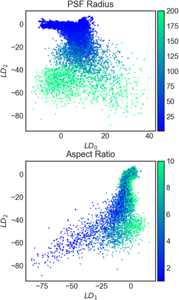
Figure 10. Effect of PSF radius and aspect ratio in a representative WST-LDA space for classification of MHD simulations. Each point comes from applying the WST to a 2D image from our MHD simulations, convolved with a PSF of the indicated radius (top) and aspect ratio (bottom), as given by the color bar. An interactive version of this figure is available at https://faun.rc.fas.harvard.edu/saydjari/RWST_2020/MHD_PSF.html, showing the PSF- and aspect ratio-dependence of the position of each point in the first three LDA coordinates. The MHD classification clusters for images containing PSF with parameters (2,1) are also shown in the LDA basis for the unblurred images, and vice versa.
Download figure:
Standard image High-resolution imageIdeally, we would find a classification space which is as insensitive as possible to the PSF. To approximate this, we take the original images, in addition to five blurred copies ((2,1), (2,2), (4,1), (4,2), (4,3)), and define the WST-LDA space for the Mach number classification task on that entire set. To better understand how the position of an image’s WST coefficients in the LDA space depend on the σ and AR of the PSFs, we take four random slices from each time step of each MHD class, and compute the WST coefficients for a Cartesian product of σ and AR. We then plot the WST coefficients corresponding to each each image with a given PSF in the space defined above in Figure 10.
39
We observe that increasing the PSF radius moves images to lower LD2, as compared to the original helical cluster. On this tail induced by the large PSF radii, the images are separated along LD1 by AR. As such, both σ and AR are encoded in the WST-LDA space. Similarly, the WST-LDA spaces for  = 0 and
  = 1 are related, but not identical, suggesting that the scale of a feature relative to the minimum pixel scale will also deform the WST-LDA space. We foresee the creation of a classifier which is invariant to, or deforms in a known way in response to, changes in the PSF and pixel scale. This is likely to be the next step before WST-LDA can be applied to classify the relevant hydrodynamic parameters (or any other parameter of interest) for observational data. It is primarily for this reason that we hold off regarding any analysis of the SFD data set, in terms of the classification space derived from the MHD simulations.
4.5. Sensitivity to Magnetic Field Direction
In the MHD turbulence simulations, the original magnetic field direction in the simulation box is topologically constrained by the periodic boundary conditions of the simulation. This introduces a preferred direction in the simulation, because the characteristics and scaling of turbulence, both parallel and perpendicular to the magnetic field, depend on the Alfvénic state of the gas (Goldreich & Sridhar 1995). The mean magnetic field remains relatively unperturbed in the sub-Alfvénic regime, in contrast to the super-Alfvénic regime, where the direction of field lines can wander (Lazarian & Vishniac 1999; Cho et al. 2002). In the simulations studied here, the mean magnetic field is initialized along the x-axis. We therefore pooled for all sub-Alfvénic MHD classes (MA = 0.7) density slices taken perpendicular to the x, y, and z axes, and show that WST-LDA picks out the x-axis, as distinct from the y- and z-axes (Figure 11). While the precision for separating x, y, and z is shown in the Figure, the fact that we find a precision of 99% for differentiating y and z from x is a more meaningful conclusion, in light of the degeneracy of y and z. For the super-Alfvénic MHD classes (MA = 2.0), WST-LDA returns a precision of only 53%. This reduced precision, as compared to the sub-Alfvénic classes, indicates that WST-LDA is sensitive to the effect of magnetic field wandering; the signatures of the magnetic field occurring in the density field for the sub-Alfvénic classes were no longer present. Thus, WST-LDA may provide an insight into the direction of homogeneous magnetic fields in the ISM.
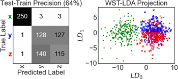
Figure 11. Confusion matrix between slices taken from the x, y, and z axes for the sub-Alfvénic MHD classes (MA = 0.7) (left). Matrix entries are the number of test images with the corresponding true-predicted label pairing. The grayscale color indicates the percentage of test images with the corresponding true label in the test set. In all cases, colors correspond to true labels, as indicated on the vertical axis in the left panel. Test and train images are plotted in the first two components of LDA space (right). Circular markers represent test images, and cross markers represent test images that were incorrectly assigned. WST-LDA can clearly distinguish the magnetic field axis, in the absence of magnetic field wandering, based solely on the density field.
Download figure:
Standard image High-resolution image5. Conclusions
We have introduced WST-LDA as a new low-dimensional classifier for non-Gaussianity. In comparison to the 3PCF, we find the WST and RWST can more readily differentiate non-Gaussian from Gaussian fields, as well as classify MHD simulation parameters. RWST-LDA appears more robust than WST-LDA to sums along the line of sight, and achieves higher precision, but is susceptible to outliers in its current form. To the best of our knowledge, this is the first classification of MHD Mach numbers in which ∼97% precision has been achieved without training a neural network. We show that the power of WST-LDA comes mostly from the number (and the relevance) of scales included in the scattering transform, rather than the number of coefficients. We similarly demonstrate 3D-WST-LDA and its application to PPV space, a case in which 3D correlations are essential to high-precision classification. Classification in PPV space may be improved by the development of anisotropic 3D wavelets preferring the velocity axis. The classification using WST-LDA was robust to additive sinusoidal noise, partial data loss, and convolution with various point-spread functions. However, the WST-LDA space in which the classification occurs was not invariant to the aforementioned effects, or to the scale of features relative to the minimum pixel scale. As such, modifying WST-LDA to be sensitive only to the MHD parameters and not to details of the resolution and pixel scale of measurements will be the next step prior to the classification of observational data.
6. Code and Data Availability
Data products associated with this paper are publicly available at doi:10.5281/zenodo.4057156 (41 GB). This includes the computed WST, RWST, and 3PCF coefficients, our selected subset of SFD, PPV density cubes from the MHD simulations, and our code for computing the 2D-3PCF. Reuse of our 3PCF code should cite Slepian & Eisenstein (2015), Slepian & Eisenstein (2016), Portillo et al. (2018), and S. Portillo et al. (2020, in preparation). Jupyter notebooks containing code to reproduce all figures in the text, some minimal working examples, and how to run these computations on a cluster are also included. The full MHD simulation runs are available from the Catalog for Astrophysical Turbulence Simulations (CATS) at http://www.mhdturbulence.com (Burkhart et al. 2020).
A.S. gratefully acknowledges the support of a National Science Foundation Graduate Research Fellowship (DGE-1745303). D.F. acknowledges the support of NSF grant AST-1614941, Exploring the Galaxy: 3-Dimensional Structure and Stellar Streams. B.B. is grateful for support from the Simons Foundation. S.K.N.P. acknowledges support from the DIRAC Institute in the Department of Astronomy at the University of Washington. The DIRAC Institute is supported through generous gifts from the Charles and Lisa Simonyi Fund for Arts and Sciences, and the Washington Research Foundation. The authors wish to thank Catherine Zucker and Michael Foley for helpful discussions. A.S. wishes to thank Sophia Sánchez-Maes for helpful discussion and much support. Computations in this paper were run on the FASRC Cannon cluster, supported by the FAS Division of Science Research Computing Group at Harvard University.
Facilities: IRAS - InfraRed Astronomical Satellite, COBE. -
Software: astropy (Astropy Collaboration et al. 2013), dustmaps (Green 2018), glue (Beaumont et al. 2015; Robitaille et al. 2017) h5py (Collette 2013), ipython (Perez & Granger 2007), kymatio (Andreux et al. 2018), matplotlib (Hunter 2007), numpy (van der Walt et al. 2011), pytorch (Paszke et al. 2019), scipy (Virtanen et al. 2020), scikit-learn (Pedregosa et al. 2012), scikit-image (van der Walt et al. 2014), yt (Turk et al. 2011).
Appendix A: Computational Costs
In order to provide an idea of the relative computational cost for each of the non-Gaussian descriptors used, we present the number of coefficients and computational time per coefficient for the 2D-WST, 3D-WST, and 3PCF (Table 1). The computation of the RWST coefficients from the WST coefficients simply involves the usual cost of least-squares optimization (and is relatively fast compared to the WST computation). Note that the definition of J for each method is slightly different. The 2D-WST, computed up to a scale, J, includes j = 0, ..., J − 1, while the 3D-WST and 3PCF include j = 0, ..., J. For the 2D and 3D-WST we used L = 8, and for the 3PCF we used L = 9. For J ≥ 7, the memory load for 3D-WST exceeds 100 MiBs, and needs to be considered. For 3D-WST and 3PCF, the coefficients were calculated on an image of uniform grid size 2J . For 2D-WST only, the computational time reflects the calculation of the coefficients on 28−J × 28−J subsets of the full 2562 images of size 2J × 2J . These experiments were executed on the FASRC Cannon cluster at Harvard University, on a computer node with water-cooled Intel 24-core Platinum 8268 Cascade Lake CPUs, with 192 GB RAM running 64 bit CentOS 7. Cascade Lake cores have dual AVX-512 fused multiply add (FMA) units. Code scaling is reported on a single core in a Python environment, specified by the yaml file in Section 6.
Table 1. Computational Cost for the 2D-WST, 3D-WST, and 3PCF
| J | Time/Coeff (core-milliseconds) | Number of Coefficients | ||||
|---|---|---|---|---|---|---|
| 2D-WST | 3D-WST | 3PCF | 2D-WST | 3D-WST | 3PCF | |
| 8 | 3.4 | 2600 | 1.2 | 1857 | 1215 | 360 |
| 7 | 1.4 | 140 | 0.95 | 1401 | 972 | 280 |
| 6 | 0.75 | 12 | 0.73 | 1009 | 756 | 210 |
| 5 | 0.47 | 1.5 | 0.56 | 681 | 567 | 150 |
| 4 | 0.30 | 0.35 | 0.39 | 417 | 405 | 100 |
| 3 | 0.23 | 0.12 | 0.27 | 217 | 270 | 60 |
Download table as: ASCIITypeset image
Appendix B: Effect of Mean Zero on 3PCF
Defining a density fluctuation field with mean zero as  , with
  being the average density, the 3PCF is

where the angle brackets denote averaging over translations and rotations. Substituting in the definition of δ, and defining the density-2PCF, as  , we find

where ζρ is the 3PCF of the density field, and we have used the identity that ∣ r 2 − r 1∣ = r3. Therefore, as claimed, taking a zero-mean field results in subtracting out the 2PCF contribution to the 3PCF.
Appendix C: RWST Angle Dependence
While we show that the RWST transformation of the WST coefficients can improve the performance of RWST-LDA, as compared to WST-LDA, the origin of this improvement is still not fully understood. To illustrate this, we compute the WST coefficients J = 2, L = 256, and M = 2 for two images measuring 16 × 16 pixels: a subset of an SFD image, and an image with random pixels. The SFD image at this pixel scale provides only an example of a real, slowly varying field, in contrast with the random image, in which neighboring pixels are totally uncorrelated. The angle dependence of the second-order WST coefficients for an internal 4 × 4 subset of pixels is shown as a function of θ1 and θ2 in Figure 12. A horizontal line cut near the top of the WST coefficient map is also shown, in order to illustrate the oscillation envelope fit by the cosine in the RWST model. While detailed aspects of the WST coefficient maps are different, both the continuously varying field and the random image display clear oscillations. In this case, we attribute the oscillations to the fact that, for all scales, the wavelets are not well sampled in the Fourier domain. It is possible that much of the relevant information enters into the amplitude of the WST coefficients, but more work is needed to understand the optimal parameterization of these oscillations, and to better understand their interpretation.
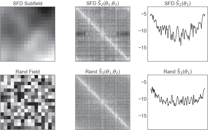
Figure 12. Images used for computing fine-angle dependence on an SFD subfield (top left) and a random pixel image (bottom left). A second-order WST coefficient map, in terms of θ1 and θ2, is shown for SFD (top middle) and Rand (bottom middle). On the right, line cuts along θ1 are plotted for SFD (top right), and Rand (bottom right), with the same y-scale, spanning the minimum and maximum  , obtained for both images.
Download figure:
Standard image High-resolution image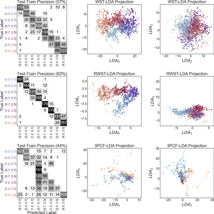
Figure 13. Confusion matrix between MHD classes, labeled with [sonic, Alfvénic] Mach numbers when applying WST-LDA (top left), RWST-LDA (middle left), and 3PCF-LDA (bottom left) for images drawn from cumulative sums along the MHD simulation density cubes. Matrix entries are the number of test images with the corresponding true-predicted label pairing. The grayscale color indicates the true positive percentage, relative to the number of test images with the corresponding true label. Test images are shown in the first two components of LDA space for the WST (top right), RWST (middle right), and 3PCF (bottom right). Circle markers represent images that were correctly assigned, and cross markers represent those that were incorrectly assigned. In all cases, colors correspond to true labels. An interactive version of this figure is available at https://faun.rc.fas.harvard.edu/saydjari/RWST_2020/MHD_LDA_cumsum.html, showing the images in 3D LDA space, and allowing isolation of the train, correctly labeled test images, and incorrectly labeled test images.
Download figure:
Standard image High-resolution imageAppendix D: Classification of Cumulative Sums
In order to mimic 2D dust maps that measure dust integrated along the lines of sight, we sampled the cumulative sum of our MHD density cubes along each axis, and repeated the classification based on sonic and Alfvénic Mach numbers, using LDA combined with the WST, RWST, and 3PCF (Figure 13). WST-LDA achieves a precision of only 54%, and shows a large broadening in the variance for each class, which leads to significant crosstalk between multiple adjacent classes. However, the confusion matrix is still predominately diagonal, with most of the density within two classes from the correct label. As such, sampling the cumulative sum can be viewed as causing an increased uncertainty in the Mach number assignments. RWST-LDA shows a much smaller decrease in precision (to 81%) and much smaller class variance on the cumulative sum images, as compared to WST-LDA. This further supports the claim that the nonlinear transformation of the WST coefficients made by the RWST is not only useful in terms of dimension reduction, but also makes the classifier more robust against variations that are uninformative with regard to distinguishing the MHD classes. While the 3PCF-LDA precision drops to approximately to 51%, near that for WST-LDA, the classification is much worse, in that many images overlap in the LDA space, and are all predicted to be in the same class. This is a function of the nonlinear spacing of classes in the 3PCF-LDA space. The comparatively poor performance of 3PCF also suggests that the specific combination of up to fourth-order moments included in the WST is well chosen, since the 3PCF alone is so strongly modified.
Footnotes
- 9
An outlier with value X will enter as Xn in the N-point correlation function.
- 10
A non-expansive operator is an operator, M, such that ∣Mx − My∣ ≤ ∣x − y∣, where ∣∣x∣∣2 = ∫∣x(u)∣2 du . In the context of the WST, M is simply the usual modulus for complex numbers, which is non-expansive by the triangle inequality. This property ensures stability to additive noise, because small changes in the field cannot cause more than the same small changes in the coefficients. Furthermore, an outlier with value X always enters the nth-order scattering coefficient proportionally to X (see Section 2.1.2).
- 11
Alfvén waves are transverse waves for which magnetic tension provides the restoring force, and the Alfvén speed scales as
 one often measures turbulent velocity magnitudes relative to the Alfvén speed.
 - 12
We verified that the real and imaginary parts of the 3PCF coefficients are even and odd under reflection as expected.
- 13
By including j = 8, triangles with large radii and large angles can probe pixels that are highly correlated in the presence of periodic boundary conditions.
- 14
The wavelet scattering transform we consider here is based on a specific instance of wavelet decomposition, which is a more general technique. In fact, a similar wavelet decomposition was previously performed on the MHD simulations we study (Kowal & Lazarian 2010), although that decomposition was not used as the basis for the WST, or as inputs for a classification algorithm.
- 15
While the maximum spatial scale is 2J , the wavelet indices refer to the wavevector (in pixels) in the Fourier domain. Thus j = J − 1 in the Fourier domain is the minimum possible scale for a spatial domain of 2J .
- 16
Note that this formal normalization is not implemented in Kymatio.
- 17
kymatio (Andreux et al. 2018) is a Python implementation of the WST, available at https://www.kymat.io.
- 18
For q = 1/2, small nonzero values are upweighted, providing a measurement of sparsity. For q = 1, the WST coefficients simply scale linearly with density. For q = 2,
interactions are upweighted. - 19
After the completion of this work, we became aware of pywst, a Python implementation of the RWST, available at https://github.com/bregaldo/pywst. Our own implementation can be found in Section 6. We compared the two implementations on the same images, and obtained similar results, except that pywst includes S0 in the RWST coefficients. Importantly, we also bound the phases to a single interval, [0,2π]. This provided improved convergence, but also introduced minor discrepancies between the coefficients obtained by the two methods, most prominently in
, , and the reference angles themselves. - 20
Previous attempts to reduce the dimensionality of the bispectrum have been made (Burkhart & Lazarian 2016), but the application was “not straightforward.”
- 21
Since the full sky is only ∼40,000 square degrees, there are only ∼200 independent patches of sky represented in this sample, with additional images coming from translations, rotations, and partial overlaps. Since the WST is not fully rotationally and translationally invariant (the subject of our upcoming work), these additional images are useful, even if partially redundant.
- 22
The density of dust in the ISM is sometimes assumed to be a log-normal distribution; as such, we also verified these results on
. - 23
A generalized Gaussian has the form
, with an FWHM of . Note that for p = 0.5 this is the Laplace distribution, and for p = 1 this is the Gaussian distribution. - 24
We confirmed that the results obtained for “SFD” do not change for apodized “SFD” images. This implies that the results for “NHC” stem from phase randomization, and are not just an effect of apodization.
- 25
We scale the coefficient inputs to PCA to have zero mean and unit variance, to account for any differences in magnitude between the coefficients.
- 26
glue (Beaumont et al. 2015; Robitaille et al. 2017) is a Python package for data visualization and linking, available at https://glueviz.org/.
- 27
We also ran parallel analyses with only the imaginary component, and a vector doubled in length, including both real and imaginary components. The imaginary component strongly resembled the real component, except that the cumulative explained variance was lower, below that explained by the RWST. Analysis with the doubled vector resembles that of the real component almost exactly.
- 28
Just as for PCA, we standard-scale the coefficients prior to LDA.
- 29
Test-train precision for real part of the 3PCF coefficients was 84%.
- 30
The correlation between slices (which are 1 pixel thick) does not fall to zero until there is a spacing of ∼50 pixels, so sampling every 8 slices does introduce correlations for samples within the same time step. This correlation necessarily reduces the effective sample size of our data set.
- 31
QDA can improve the precision to 96%, which is to be expected, given the high heteroscedasticity.
- 32
Recalling the 2D-WST convention that j runs from 0 to J − 1.
- 33
While we only present the q = 1 results in Figure 7 for the purpose of comparison with 2D-WST, we find that q = 1/2 slightly outperforms q = 1 for all j except j = 3, while q = 2 underperforms compared to q = 1 for all j. The choice of q (or a set of q) used with the WST may be an important optimization for difficult classification problems.
- 34
We note that the multipole expansion of
used for the 3PCF has one more angular component, as compared to 2D-WST with the same L. Excluding the zero-frequency component, the multipole expansion with contains the angular frequencies 2π/n for n for an integer from 1 to . For 2D-WST, the number of angular divisions between −π/2 and π/2 sets the Nyquist frequency to π/L. Since the angular scales for 3PCF and 2D-WST are not identical, we simply compare the number of coefficients. - 35
Similar results were obtained for y- and z-velocity field PPV cubes.
- 36
J = 7 for the 3D-WST provided too few samples for a reliable test-train split.
- 37
While the velocity axis and position axes do not even have the same units, the fractional extent of each axis captured by the wavelet represents the same fraction of the relevant range of spatial or velocity coordinates. The velocity axis of each cube is normalized to be −3 to 3σv , where σv is the velocity dispersion.
- 38
One of the authors detected a Maui radio station with a Panoramic Survey Telescope and Rapid Response System (Pan-STARRS) CCD.
- 39
We do not scale the WST coefficients to have mean zero and unit variance prior to computing the LDA space, so that we can more easily study which coefficients are most affected by the PSF.

![${\left[\mathrm{density}\right]}^{2}$](https://content.cld.iop.org/journals/0004-637X/910/2/122/revision2/apjabe46dieqn16.gif)


![$\mathrm{log}\left[\mathrm{density}\right]$](https://content.cld.iop.org/journals/0004-637X/910/2/122/revision2/apjabe46dieqn27.gif)

![$2{[2\mathrm{log}(2)]}^{1/2p}\sigma $](https://content.cld.iop.org/journals/0004-637X/910/2/122/revision2/apjabe46dieqn29.gif)


