Abstract
We present 850 μm linear polarization and C18O (3 − 2) and 13CO (3 − 2) molecular line observations toward the filaments (F13 and F13S) in the Cocoon Nebula (IC 5146) using the JCMT POL-2 and Heterodyne Array Receiver Program instruments. F13 and F13S are found to be thermally supercritical with identified dense cores along their crests. Our findings include that the polarization fraction decreases in denser regions, indicating reduced dust grain alignment efficiency. The magnetic field vectors at core scales tend to be parallel to the filaments, but disturbed at the high density regions. Magnetic field strengths measured using the Davis–Chandrasekhar–Fermi method are 58 ± 31 and 40 ± 9 μG for F13 and F13S, respectively, and it reveals subcritical and sub-Alfvénic filaments, emphasizing the importance of magnetic fields in the Cocoon region. Sinusoidal C18O (3 − 2) velocity and density distributions are observed along the filaments’ skeletons, and their variations are mostly displaced by ∼1/4 × the wavelength of the sinusoid, indicating core formation occurred through the fragmentation of a gravitationally unstable filament, but with shorter core spacings than predicted. Large-scale velocity fields of F13 and F13S, studied using 13CO (3 − 2) data, present a V-shape transverse velocity structure. We propose a scenario for the formation and evolution of F13 and F13S, along with the dense cores within them. A radiation shock front generated by a B-type star collided with a sheet-like cloud about 1.4 Myr ago. The filaments became thermally critical due to mass infall through self-gravity ∼1 Myr ago, and subsequently, dense cores formed through gravitational fragmentation, accompanied by the disturbance of the magnetic field.
Original content from this work may be used under the terms of the Creative Commons Attribution 4.0 licence. Any further distribution of this work must maintain attribution to the author(s) and the title of the work, journal citation and DOI.
1. Introduction
Filamentary molecular clouds and dense cores are known as sites of ongoing star formation, and the formation mechanisms of filaments and dense cores have been investigated through simulations and observations over the last few decades. For filament formation, simulation studies reveal that filaments emerge in gravitationally unstable infinite sheets and at the intersections of colliding turbulent sheets. Their formation and evolution are aided by the influence of the magnetic field, mechanical feedback, and radiation feedback from the surrounding clouds (see Chapter 5 of Hacar et al. 2023, and references therein). Abe et al. (2021) categorized filament formation mechanisms into five types: (i) a type G filament forms by self-gravitational fragmentation in a shock-compressed sheet-like cloud, (ii) a type I filament forms at the intersections of two sheets, (iii) a type O filament is made by the curved magnetohydrodynamic shock wave, (iv) a type C filament forms by converging gas flow along the magnetic field lines in the post-shock layers, and (v) a type S filament is formed when a small clump is stretched by turbulent shear flows. This indicates that the filament formation mechanism is closely related to the environment as well as the energy budget of turbulence, magnetic field, and gravity of the molecular cloud where the filament is created.
Expanding H i shells, primarily formed by supernovae or H ii regions, are suggested to provide sites for the formation of molecular filaments by observation and simulation studies (e.g., Dawson et al. 2008; Hennebelle et al. 2008; Inutsuka et al. 2015; Bracco et al. 2020). According to our current understanding, the large-scale shock compression resulting from multiple expanding shells can lead to the formation of flattened layers of molecular gas, with subsequent mass flows, driven by self-gravity or along magnetic fields, contributing to the creation of supercritical filamentary structures (Pineda et al. 2022).
In this context, the core formation can be modeled as the gravitational fragmentation of an isothermal equilibrium cylinder (e.g., Inutsuka & Miyama 1992), although magnetic field and turbulence can also affect the formation of cores (e.g., Seifried & Walch 2015; Clarke et al. 2016; Hanawa et al. 2017). Hence, observations toward filaments and dense cores have been performed to reveal the density and gas kinematic properties as well as the magnetic fields to examine their formation process (e.g., Hacar et al. 2018; Arzoumanian et al. 2019; Wang et al. 2022; Shimajiri et al. 2023).
IC 5146, also known as the Cocoon Nebula, is a nearby star-forming molecular cloud. The cloud exhibits a reflection nebula in the east, the Cocoon Nebula, and a dark cloud comprising multiple filaments in the west, referred to as the dark Streamer (Figure 1). Due to their proximity in the plane of the sky, the Cocoon Nebula and the dark Streamer are generally studied together. However, the Cocoon Nebula and the dark Streamer have different star-forming environments. Cocoon Nebula has ∼100 young stellar objects (YSOs), while the dark Streamer has only ∼20 YSOs (Harvey et al. 2008). Also, a single B0 V star BD+46° 3474 (hereafter BD+46) resides at the center of Cocoon Nebula (e.g., Herbig & Reipurth 2008; García-Rojas et al. 2014), surrounded by the H ii region known as Sharpless 125 (S125; Sharpless 1959). Based on optical and H i observations, it has been reported that BD+46 and the H ii region are situated in front of the parent molecular cloud, suggesting that BD+46 likely formed first and created an ionized cavity, and the stars within the IC 5146 generated in a dense region of the molecular cloud located in the foreground, which subsequently dissipated after the emergence of BD+46 (e.g., Roger & Irwin 1982; Herbig & Dahm 2002).
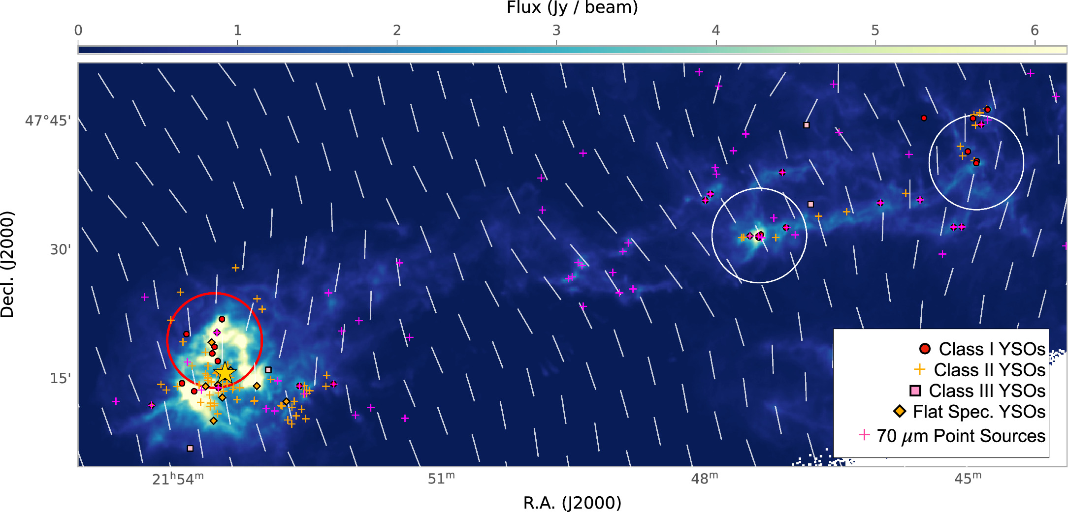
Figure 1. Herschel 250 μm image of IC 5146 (André et al. 2010). The red circle on the east is the filament-13 (F13) studied in this paper, and the white circles on the west indicate the E-hub) and the W-hub of the dark Streamer of IC 5146, which have been observed with JCMT/POL-2 (Wang et al. 2019; Chung et al. 2022). YSOs identified by Spitzer (Harvey et al. 2008) and 70 μm point sources by the Herschel/PACS Point Source Catalog (HPPSC; Poglitsch et al. 2010) are presented. The big yellow star indicates the position of a B0 V star BD+46° 3474 (BD+46). The white segments represent the magnetic field orientations inferred from the Planck 353 GHz polarization data (Planck Collaboration et al. 2016).
Download figure:
Standard image High-resolution imageThe infrared dust continuum data reveal complex filamentary structures harboring most prestellar cores of IC 5146 (Arzoumanian et al. 2011). Chung et al. (2021) investigated the filaments and dense cores in IC 5146 with C18O (1 − 0) and N2H+ (1 − 0) molecular line data, and found that most dense cores are located on the gravitationally supercritical filaments of IC 5146. Interestingly, the N2H+ emission, known as one of the useful tracers of dense cores, is detected throughout the filaments of the dark Streamer, but it is merely detected in the filaments of the Cocoon Nebula. The filaments in the Cocoon Nebula have similar gravitational criticality to those of filaments in the dark Streamer, while they have slightly smaller nonthermal velocity dispersions normalized by the local sound speed than the filaments in the dark Streamer. Hence, Chung et al. (2021) suggested that the thermal pressure and/or magnetic field support may be more significant in the filaments of the Cocoon Nebula than in those of the dark Streamer.
The magnetic field structures in IC 5146 have been studied by polarization observations at various wavelengths (e.g., Planck Collaboration et al. 2016; Wang et al. 2017, 2019; Chung et al. 2022). The large-scale magnetic fields appear to be nearly uniform and perpendicular to the elongated orientation of the IC 5146 Streamer (e.g., Planck Collaboration et al. 2016). However, on the core scale, the magnetic field orientations are revealed to be more complex. The white circles in Figure 1 show the eastern hub (E-hub) and western hub (W-hub) of the dark Streamer where the magnetic fields have been investigated using the JCMT POL-2 polarimetry (Wang et al. 2019; Chung et al. 2022). The E-hub has a curved B field indicating a possible drag by the gravitational contraction (Wang et al. 2019). Meanwhile, the W-hub, which is likely more fragmented and evolved than the E-hub, shows much more complex B-field orientations (Chung et al. 2022). The B field strength of the W-hub is 0.6 ± 0.2 mG, and that of the E-hub is 0.3 ± 0.1 mG (recalculated in the same manner as that of the W-hub by Chung et al. 2022). Although both hubs are magnetically supercritical, the E- and W-hubs are found to have slightly different fractions of gravitational (EG), turbulent (EK), and magnetic (EB) energy. This implies that the importance of magnetic field, turbulence, and gravity may change as filaments and dense cores evolve within different environments.
Recently, Wang et al. (2020) used GAIA DR3 data to measure the distances to the Cocoon Nebula of 813 ± 106 pc and to the dark Streamer of 600 ± 100 pc. The distance of BD+46 is reported to be 800 ± 80 pc (García-Rojas et al. 2014), being well consistent with that of the Cocoon Nebula (Wang et al. 2020).
We carried out SCUBA-2/POL-2 and Heterodyne Array Receiver Program (HARP) observations toward the filamentary cloud regions in the Cocoon Nebula (the red circle area in Figure 1), which consist of three filaments (named F13, F13S, and F13W). These filaments are reported as thermally supercritical and sub/transonic, and no N2H+ emission is detected for these regions (Chung et al. 2021). This filament system is thought to be a good laboratory to investigate the formation mechanism of filament and dense cores as having a different environment from that of the dark Streamer.
The paper is organized as follows. We describe the observations and data reductions in Section 2, and give the results of the observations in Section 3. We analyze and discuss in Sections 4 and 5, respectively. We summarize our results in Section 6.
2. Observations
2.1. Polarization Observations
Polarization observations were carried out with the JCMT POL-2 polarimeter between 2021 June 9 and 2022 August 9. The observations were performed toward F13 in the Cocoon Nebula using the standard SCUBA-2/POL-2 daisy mapping mode, which covers the observing total area of a diameter  with its central area of a diameter
  having the best sensitivity. Its angular resolution is 14
1 at 850 μm wavelength (corresponding to ∼0.056 pc at a distance of 813 pc). The observations were made 21 times and the integration time of each observation was about 40 minutes, resulting in a total on-source time of ∼14 hr under dry weather conditions with submillimeter opacity at 225 GHz (τ225GHz) ranging between 0.05 and 0.08.
We used the pol2map routine in the Sub-Millimeter User Reduction Facility (SMURF) package of the Starlink software. Initially, the raw bolometer time streams are converted into Q, U, and I time streams using the calcqu command and I time streams of each observation are generated from the makemap command. In this process, a mask determined by the signal-to-noise ratio (S/N) is used. Then, a pointing correction is applied and a mask determined from the co-added I map is used to generate an improved I map. Finally, Q and U maps are produced from their time streams using the same mask in the previous step, and a final vector catalog is created. The final I, Q, and U maps have a bin size of 4″, and the vector catalog binned to 12″ is used.
The “2019 August” IP model
7
was applied for the instrumental polarization correction. A flux calibration factor (FCF) of 668 Jy pW−1 beam−1 is used for the 850 μm Stokes I, Q, and U data. The FCF is determined from the standard 850 μm SCUBA-2 flux conversion factor of 495 Jy pW−1 beam−1 by multiplying a correction factor of 1.35 for the additional losses from POL-2 (Mairs et al. 2021). The mean rms level in Stokes I is 4.0 mJy beam−1, and the best rms level within the central  region is 3.5 mJy beam−1.
2.2. Molecular Lines Observations
C18O and 13CO (3 − 2) molecular line observations toward F13 filaments by using JCMT HARP (Buckle et al. 2009) were performed to estimate their velocity centroids and dispersions. The main beam efficiency is 0.64 at 345 GHz (Buckle et al. 2009). The data were taken using basket-weaved scan maps toward the central  area between 2022 August 8 and September 1 in weather band 3 (0.08 < τ225GHZ < 0.12). The total observation time is 7.1 hr. The spatial and spectral resolutions for the C18O and 13CO (3 − 2) observations are about 14″ and 0.05 km s−1, respectively.
We used the REDUCE_SCIENCE_NARROWLINE recipe of the ORAC-DR pipeline in the Starlink software. To increase the S/N, we resampled the data cube to a channel width of 0.1 km s−1 with a one-dimensional Gaussian kernel. The pixel size and the mean rms level of the final data cube are 73 and about 0.06 K
![$[{T}_{{\rm{A}}}^{* }]$](https://content.cld.iop.org/journals/0004-637X/970/2/122/revision1/apjad4f85ieqn5.gif) , respectively.
, respectively.
3. Results
Figure 2 shows the Herschel H2 column density map obtained from the Herschel Gould Belt survey 8 (HGBS; André et al. 2010; Arzoumanian et al. 2011) with 850 μm Stokes I contours. The crests of filaments found from DisPerSE 9 are presented with solid curves (Arzoumanian et al. 2011). They can be separated into three parts. We refer to the main filament as F13 following its discovery by Chung et al. (2021), while the remaining two as F13S and F13W based on their relative positions to F13. F13 exhibits the highest H2 column density, followed by F13S and F13W, with a decreasing density. The 850 μm Stoke I emissions show a good overall agreement with Herschel’s H2 column density distribution. Especially, the peak positions of 850 μm emission in F13 and F13S are well consistent with the H2 column density peaks.
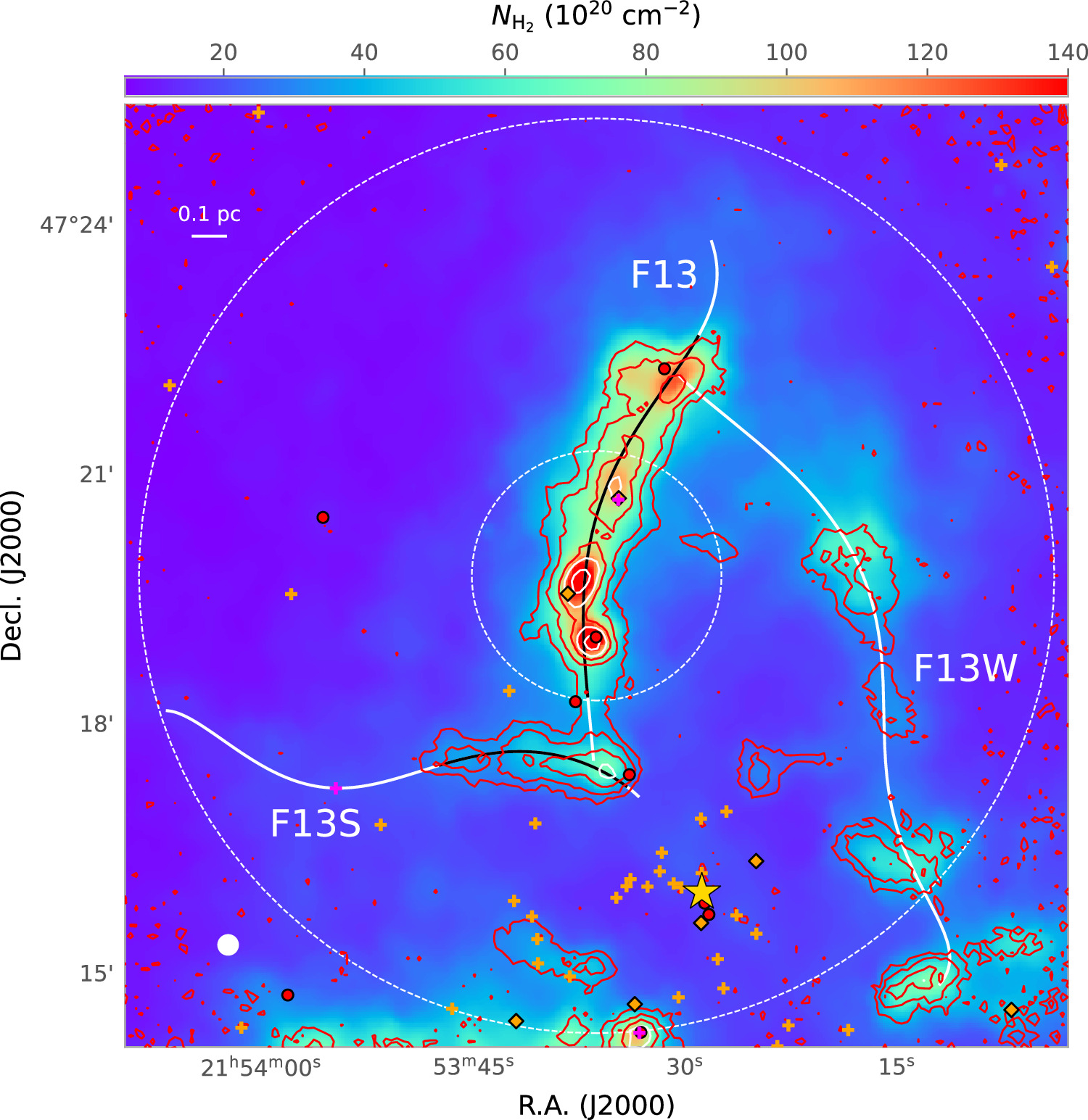
Figure 2. 850 μm Stokes I map (red contours) on the H2 column density map from the Herschel data (color tone; Arzoumanian et al. 2011). The contour levels of 850 μm emission are 3, 10, 20, 30, and 50 × σ (1σ = 4.0 mJy beam−1). The yellow star in the south indicates the position of BD+46. The positions of YSOs identified by Spitzer (Harvey et al. 2008) and 70 μm point sources by the HPPSC; (Poglitsch et al. 2010) are presented the same as in Figure 1. The dashed circles indicate the full area of POL-2 daisy map mode, which covers a circular region of  diameter and the best sensitivity coverage of central
  of the map, respectively. The white circle at the bottom left corner shows the POL-2 850 μm beam size of 14
1. The white curves present the crest of the filament identified from the Herschel H2 column density data by Arzoumanian et al. (2011), which are named F13, F13S, and F13W following Chung et al. (2021), and the black curves on them are the region where the data are analyzed in this paper.
Download figure:
Standard image High-resolution image3.1. Filaments and Dense Cores
We identified dense cores by applying the FellWalker source extraction algorithm (Berry 2015) to the 850 μm Stoke I map. During the execution of this algorithm, we considered pixels with intensities higher than 0.5σ to identify all dark cores. To classify an object as a genuine core, we set the minimum peak intensity threshold to 10σ and the size threshold to three times the beam size of 141. We used 1.5σ as the minimum dip threshold, which determines the neighboring peaks to be separated if the difference between the peak values and the minimum value (dip value) between the peaks is larger than the given threshold. From this, four and three cores were found in F13 and F13S, respectively. The cores in F13 are named C1–C4 from south to north, and those in F13S are named C5– C7 from east to west.
The identified cores are represented with ellipses over H2 column density map provided by Arzoumanian et al. (2011) in Figure 3(a) and their positions on the crest are marked with vertical lines over the longitudinal H2 column density profile in Figures 3(b) and (c). As shown in the Figure, the 850 μm cores are well fitted with the  peak positions. The mean projected separations of cores in F13 and F13S are 0.27 ± 0.08 and 0.20 ± 0.05 pc, respectively.
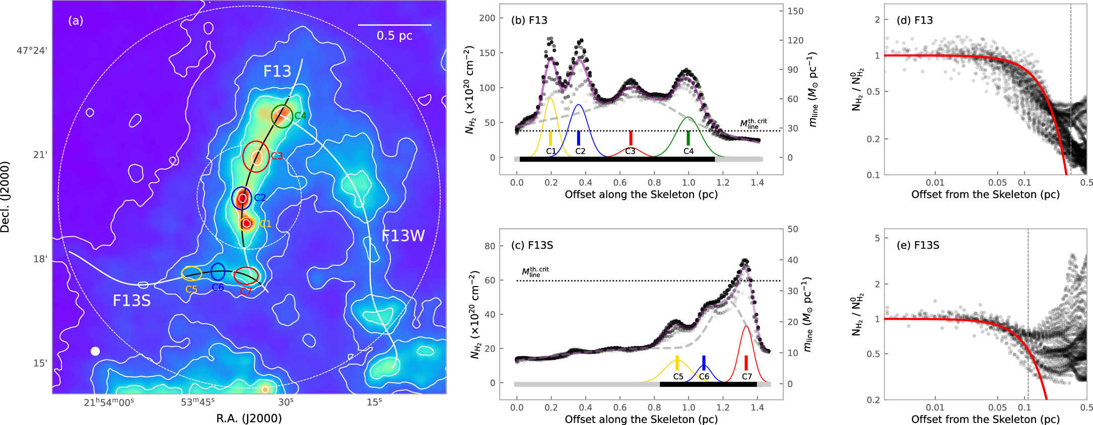
Figure 3. Longitudinal and radial H2 column density profiles of F13 and F13S. (a) Herschel H2 column density map (Arzoumanian et al. 2011). The color scale and curves are the same as that in Figure 2 and the contour levels are the H2 column densities of 10, 20, 30, 50, 100, and 150 × 1020 cm−2. The colored ellipses indicate the cores identified with FellWalker. (b) and (c) Longitudinal H2 column density profiles along the crest from south to north for F13 and from east to west for F13S, considering only pixels located at a distance <0.05 pc from the crest. The colored curves represent the Gaussian models for the dense cores, while the thick dashed gray curve corresponds to the background filament material. The thick purple curve represents the sum of the Gaussian models and the filament material. The colored vertical segment indicates the peak position of the core’s Gaussian model. On the right y-axis, the corresponding local line mass (mline) is presented, and the dotted horizontal lines indicate the thermal critical line mass ( ) at the mean temperature (please refer to the relevant text for more details). (d) and (e) Normalized radial column density profiles centered on the crest of filament and their Gaussian fits to estimate the filaments’ widths. The Gaussian fits were performed only for the points in r ≤ rth, where rth is 0.33 and 0.11 pc for F13 and F13S, respectively. The red curve displays the Gaussian fit result and the vertical dashed line depicts the offset from the skeleton where r = rth.
Download figure:
Standard image High-resolution imageWe estimated the physical quantities of F13 and F13S using the Herschel column density map. We measured the filament’s length along the crest given by Arzoumanian et al. (2011) within the enclosed region of  for F13 and
  for F13S (depicted with black curves in Figures 3(a)–(c)). The lengths of F13 and F13S are 1.13 ± 0.09 and 0.56 ± 0.05 pc, respectively. The length of F13 identified with the C18O (1 − 0) molecular line data is 1.01 pc (Chung et al. 2021), which is comparable to that measured in this study.
As shown in Figures 3(b) and (c), the range of  on the crest (
 ) of F13 is about 50–170 × 1020 cm−2 and that of F13S is about 30–70 × 1020 cm−2. The mean
  (
( ) of F13 and F13S are ∼93 ± 27 and ∼42 ± 12 × 1020 cm−2, respectively.
To measure the filaments’ widths (W), we used the normalized radial column density profiles ( ) as presented in Figures 3(d) and (e). The profiles show a smooth decrement of column density with the increasing radial distance and some bumps at r ≳ 0.2 pc. The bumps are due to the substructure near C4 in the case of F13 and due to the other filament materials at the junctions of F13S and F13 as well as F13 and F13W in Figure 3(a). To avoid the effect of other filament materials on the measurement, we set the threshold radius (rth) and performed Gaussian fitting only for the points at r ≤ rth. We applied rth = 0.33 and 0.11 pc for F13 and F13S, respectively, at the point where
  begins to increase as the distance grows. The widths are estimated from the FWHM of the Gaussian (Wuncorr) by correcting the beam smearing effect (
 where θbeam = 14
1), and W are 0.32 ± 0.07 and 0.23 ± 0.03 pc for F13 and F13S, respectively. These values are slightly larger than or similar to those obtained with the C18O (1 − 0) molecular line data (0.26 pc; Chung et al. 2021).
The mass per unit length (Mline = M/L) is commonly examined as an indicator of filament instability, similar to the Jeans mass for spherical systems. On the right y-axis of Figures 3(b) and (c), we presented the corresponding local line mass (mline) estimated from the H2 column density by multiplying the filament width ( ). The line mass is found to range between ∼10 and 120 M⊙ pc−1. In a hydrostatic isothermal cylinder model, the critical line mass (
 ) represents the equilibrium point where the thermal pressure balances with the gravitational collapse. It can be calculated using the equation

where cs
is the sound speed (Ostriker 1964). At the mean dust temperatures of 19.8 ± 1.2 and 24.2 ± 1.0 K of F13 and F13S regions,  of F13 and F13S are ∼27 ± 2 and 33 ± 1 M⊙ pc−1, respectively. The local line mass of F13 is found to be larger than the critical line mass along the entire crest, whereas that of F13S is higher than the critical line mass only near the westernmost core (C7).
We measured the H2 number density ( ) of each filament by assuming the cylindrical geometry of the filament having a diameter of estimated width.
  at the distance, r, from the skeleton is calculated with the following equation:

where the line-of-sight length, llos, is

where W is the filament’s width. The estimated H2 number densities along the skeleton of F13 and F13S range 8–17 × 103 and 6–8 × 103 cm−3, respectively. The mean values ( ) are 11 ± 2 × 10³ and 7 ± 1 × 103 cm−3 for F13 and F13S, respectively. The calculated physical parameters of filaments are listed in Table 1.
Table 1. Physical Parameters of the Filaments
| Tdust | L | W |

|

| M | Mline |

| σNT | |
|---|---|---|---|---|---|---|---|---|---|
| (K) | (pc) | (1020 cm−2) | (103 cm−3) | (M⊙) | (M⊙ pc−1) | (km s−1) | |||
| F13 | 19.8 ± 1.2 | 1.13 ± 0.09 | 0.32 ± 0.07 | 93 ± 27 | 11 ± 2 | 76 ± 28 | 67 ± 24 | 27 ± 2 | 0.30 ± 0.04 |
| F13S | 24.2 ± 1.0 | 0.56 ± 0.05 | 0.23 ± 0.03 | 42 ± 12 | 7 ± 1 | 12 ± 4 | 22 ± 7 | 33 ± 1 | 0.29 ± 0.05 |
Download table as: ASCIITypeset image
3.2. Polarization Properties
Using the obtained Q and U maps, polarization intensity (PI), polarization fraction (P), and polarization angle (PA) were obtained. PI is the quadratic sum of Q and U ( ), and the noises of Q and U always make a positive bias in PI and P (Vaillancourt 2006). Hence, a correction was performed with the modified asymptotic estimator (Plaszczynski et al. 2014) and the debiased polarization intensity was estimated with the following equation:

The noise bias σ is calculated from the following equation (Plaszczynski et al. 2014):

where σQ and σU are the standard errors in Q and U, respectively.
The debiased polarization fraction P was measured by

and its uncertainty was calculated by propagating the standard errors of PI (σ) and I (σI ) with the equation of

The polarization position angle, θ, can be calculated by

from the definition of Q and U parameters of

and

The uncertainty of θ was calculated by the equation (e.g., Ngoc et al. 2021):

Figure 4 shows the polarization vectors on the Stokes I image. With the selection criteria of I/σI ≥ 10 and P/σP ≥ 2, 94 vectors are obtained (51 vectors having P/σP ≥ 3). One noticeable feature is that the polarization vectors are mostly perpendicular to the skeletons of filaments, especially in F13S and F13W. The polarization fractions appear to be lower in the brighter region.
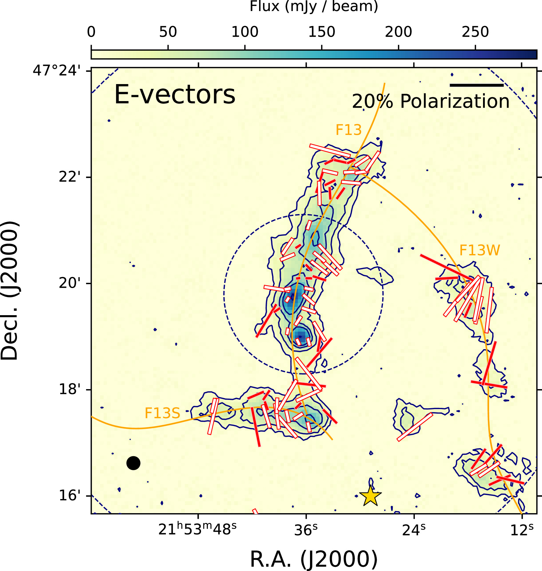
Figure 4. The polarization segments on the 850 μm Stokes I intensity map (color scale and contours). The segments are selected with the criteria I/σI ≥ 10 and P/σP ≥ 2. The white and red bars are for the polarization vectors with 2 ≤ P/σP < 3 and P/σP ≥ 3, respectively. A 20% line segment is presented for reference in the top right corner. The black circle at the bottom left corner is the POL-2 850 μm beam size of 141. The orange curves are the skeletons of filaments and the yellow star indicates the position of BD+46.
Download figure:
Standard image High-resolution imageIt is well known that the polarization fraction tends to decrease as the intensity increases with a power-law relation of P ∝ I−α (e.g., Whittet et al. 2008; Pattle et al. 2019). Dust polarization is observed likely because of the nonspherical shape of dust grains and the alignment of their minor axes parallel to the local magnetic field. The polarization fraction is related to the alignment efficiency of the dust grains, which may be determined by the size and composition of the dust. It is quite complex to infer the dust alignment efficiency from the observed polarization fraction because it can be affected by the dust opacity and the mixing of various magnetic fields with different strengths and geometry along the line-of-sight direction. However, it still gives important information on the dust alignment efficiency, and the power-law index α is useful to demonstrate the polarization properties of a cloud. α = 0 implies that the dust in a cloud has the same alignment efficiency at all optical depths. α = 0.5 means that the efficiency of dust alignment linearly decreases as the optical depth increases. α = 1 is observed if the dust grains align only at the thin surface layer of the cloud but no dust grains align at higher densities (e.g., Whittet et al. 2008).
We presented the relationship between the intensity and polarization fraction in Figure 5. The left panel shows the debiased polarization fraction (Pdb) as a function of the normalized I intensity divided by σQU
(the mean of σQ
and σU
). We performed a least squares single power-law fit of  , where σQU
is the representative rms noise in Stokes Q and U (and the reference intensity), and
, where σQU
is the representative rms noise in Stokes Q and U (and the reference intensity), and  is the polarization fraction at the reference intensity (σQU
). The fit results with vectors of I/σI
≥ 10 and with those of I/σI
≥ 10 and P/σP ≥ 3 are overlaid with dashed and solid lines, respectively. The power-law index α of the fit using the polarization segments of I/σI
≥ 10 and P/σP ≥ 3 is 0.82 ± 0.09.
is the polarization fraction at the reference intensity (σQU
). The fit results with vectors of I/σI
≥ 10 and with those of I/σI
≥ 10 and P/σP ≥ 3 are overlaid with dashed and solid lines, respectively. The power-law index α of the fit using the polarization segments of I/σI
≥ 10 and P/σP ≥ 3 is 0.82 ± 0.09.
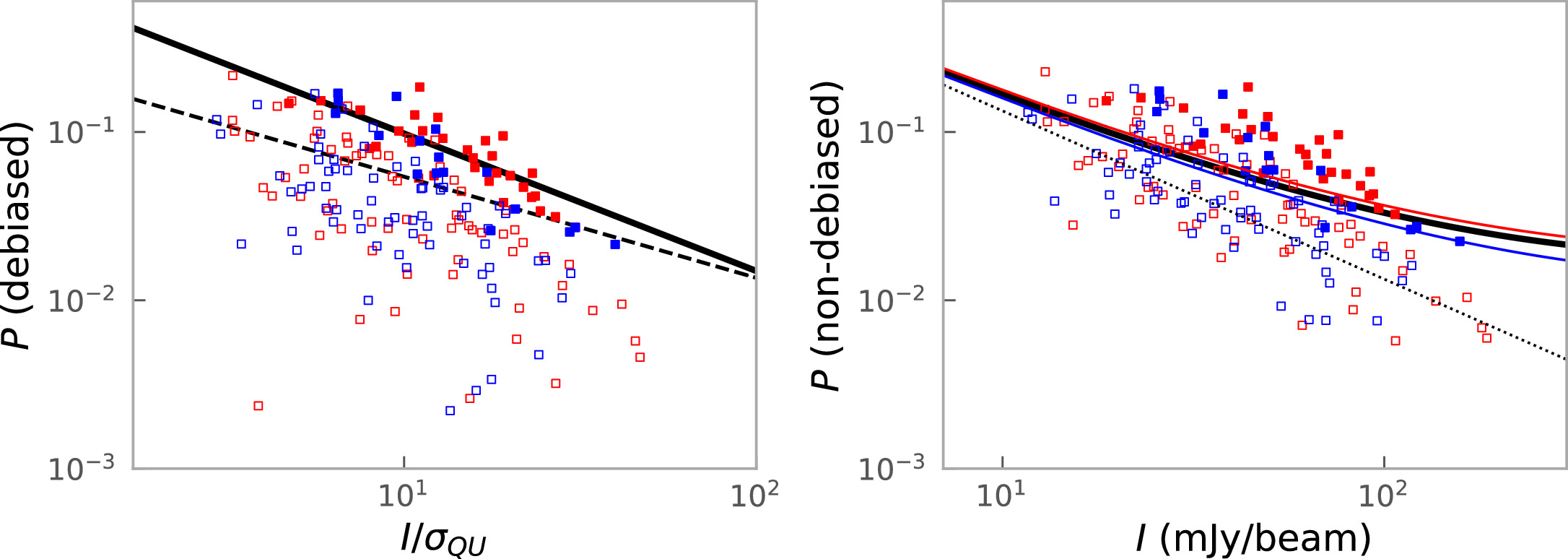
Figure 5. Relationship between the polarization fraction and the Stokes I intensity. The open and filled squares denote the polarization segments with P/σP < 3 and P/σP ≥ 3, respectively. The red and blue squares indicate the vectors of closer and far regions, respectively (see Section 5.1). Left: the debiased polarization fraction as a function of the normalized Stoke I intensity by σQU
(the mean of σQ
and σU
). The dashed and solid lines are the best fit to a single power-law function,  , with polarization segments of I/σI
≥ 10 and those of I/σI
≥ 10 and P/σP ≥ 3, respectively. Right: relationship between the non-debiased polarization fraction and the Stokes I intensity. The solid black line is the best-fit Ricean-mean model with all the polarization segments, and the dotted line is the null hypothesis case (α = 0). The red and blue curves are the best-fit Ricean-mean model with the vectors of closer and far regions from the BD+46, respectively.
, with polarization segments of I/σI
≥ 10 and those of I/σI
≥ 10 and P/σP ≥ 3, respectively. Right: relationship between the non-debiased polarization fraction and the Stokes I intensity. The solid black line is the best-fit Ricean-mean model with all the polarization segments, and the dotted line is the null hypothesis case (α = 0). The red and blue curves are the best-fit Ricean-mean model with the vectors of closer and far regions from the BD+46, respectively.
Download figure:
Standard image High-resolution imageWe also obtained α using the Ricean-mean model (Pattle et al. 2019). The single power-law model is appropriate for the data with a high S/N, but it is not valid for the low S/N data where the observed polarization fraction follows a Rice distribution, and thus α may be overestimated (Pattle et al. 2019). The Ricean-mean model was adopted to show that α can be well recovered by this model. We applied the Ricean-mean model to the non-debiased data with I/σI ≥ 10 following the equation (Pattle et al. 2019):

where  is a Laguerre polynomial of order 1/2.
The right panel of Figure 5 shows the relationship between the non-debiased polarization fraction and the Stokes I intensity with the best-fit Ricean-mean model. The obtained α and  are 0.72 ± 0.07 and 0.33 ± 0.08, respectively. The fitting results are tabulated in Table 2.
Table 2. Fitting Results of the Single Power-law Function and the Ricean-mean Models
| Single Power-law model | Ricean-mean model | |||
|---|---|---|---|---|

| α |

| α | |
| Vectors with I/σI ≥ 10 and P/σP ≥ 3 | 0.64 ± 0.14 | 0.82 ± 0.09 | … | … |
| Vectors with I/σI ≥ 10 | … | … | 0.33 ± 0.08 | 0.72 ± 0.07 |
| Close to BD+46 a | … | … | 0.38 ± 0.10 | 0.73 ± 0.07 |
| Far from BD+46 a | … | … | 0.29 ± 0.14 | 0.71 ± 0.13 |
Note.
a We divided the vectors into two groups based on their positions within the filaments, one group close to and the other group further away from the B-type star with respect to the skeleton of the filament.Download table as: ASCIITypeset image
The expected α for the molecular clouds ranges between 0.5 and 1. The molecular clouds studied in the BISTRO survey have α of 0.8−1.0 with a single power-law model. α obtained from the Ricean-mean model of the BISTRO objects ranges between 0.3 and 0.7 (e.g., Pattle et al. 2019; Wang et al. 2019; Arzoumanian et al. 2021; Lyo et al. 2021; Ching et al. 2022; Hwang et al. 2022).
The obtained α of the Cocoon Nebula from a single power-law function as well as from the Ricean-mean model lie well between the expected range of molecular cloud. α from a single power-law function for the vectors having I/σI ≥ 10 and P/σP ≥ 3 is quite close to that of the early B-type star LkHα 101 region. On the contrary, α from the Ricean-mean model falls on the higher end of the BISTRO’s range. We discuss the relationship between I and P in Section 5.1.
3.3. Velocity Field from the C18O and 13CO (3 − 2) Data
Figure 6 presents the C18O (3 − 2) moment maps. The integrated intensity map shows that the distribution of C18O emission is well matched to that of 850 μm emission in F13, but in the F13S region, it is detected only at the dense western part.
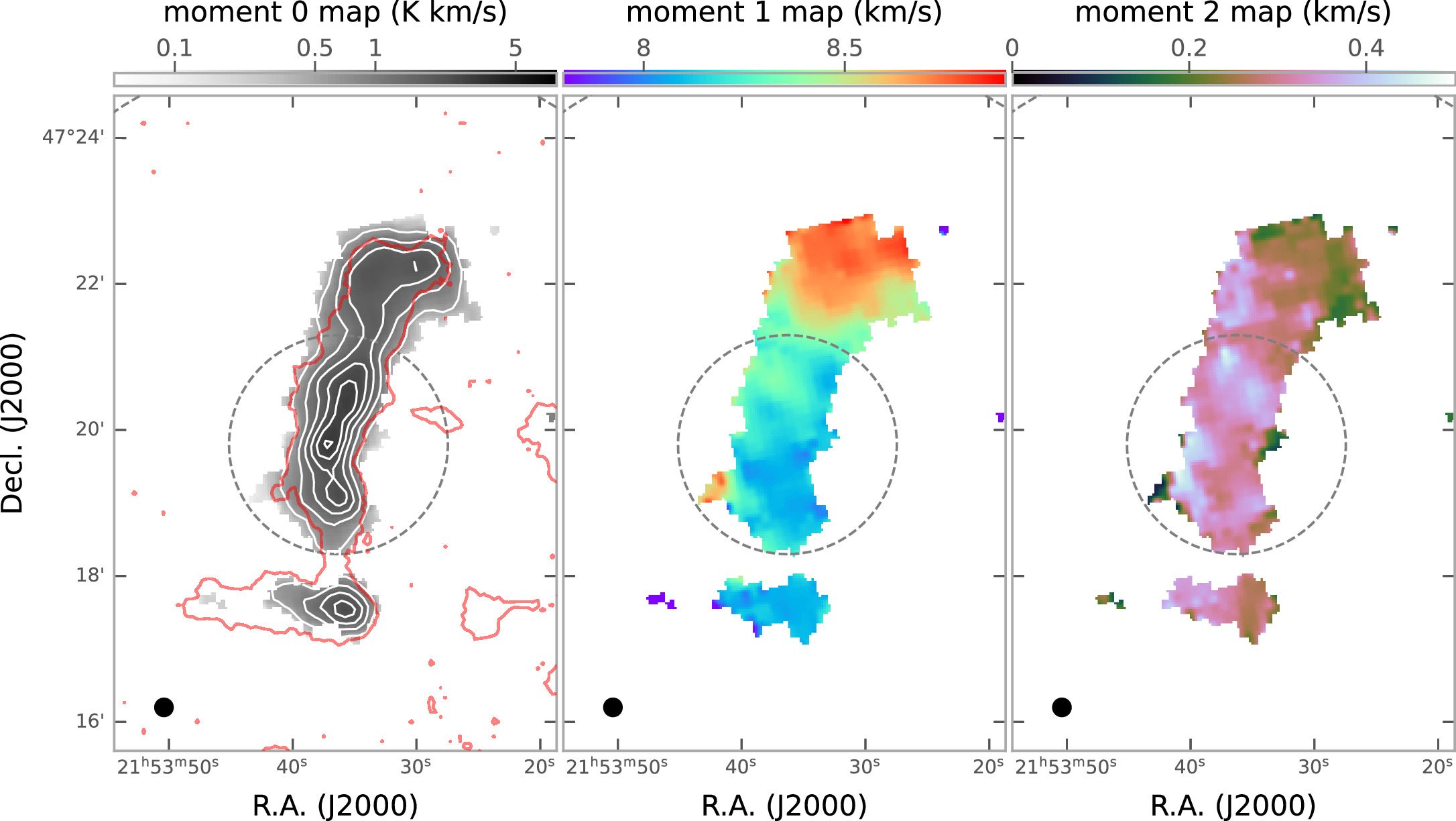
Figure 6. C18O (3 − 2) moment maps obtained from the HARP instrument of JCMT. In the moment 0 map, the integrated intensity contours of C18O are drawn with white color and the contour levels are 10, 20, 30, ⋯, 60 × σ (σ = 0.053 K km s−1). The red contour is the 3σ level of the 850 μm Stokes I intensity. The spatial resolution is 14″, and the beam is given at the bottom left panel of the maps.
Download figure:
Standard image High-resolution imageThe moment 1 map reveals a gradual increase in velocity, ranging from approximately 7.7 km s−1 in the southeast, 8.0 km s−1 in the south, to 8.8 km s−1 in the north. The mean velocity gradient of F13 is ∼0.9 km s−1 pc−1 and that of F13S is ∼1.0 km s−1 pc−1. The velocity dispersions are in a range between ∼0.2 and 0.6 km s−1 with a mean value of 0.30 ± 0.06 km s−1. We inspected the spectra and discovered that all of them exhibit a single velocity component.
Figure 7 presents the C18O (3 − 2) velocity structure along the skeleton of F13 and F13S. F13 exhibits a globally increasing velocity field from south to north, but with small oscillatory behaviors. The dotted vertical lines depict the cores’ positions, and the velocity decreases and then increases around C3 up to C4 position along the skeleton from south to north. In contrast, around the other cores, such abrupt changes in velocity direction are not observed.
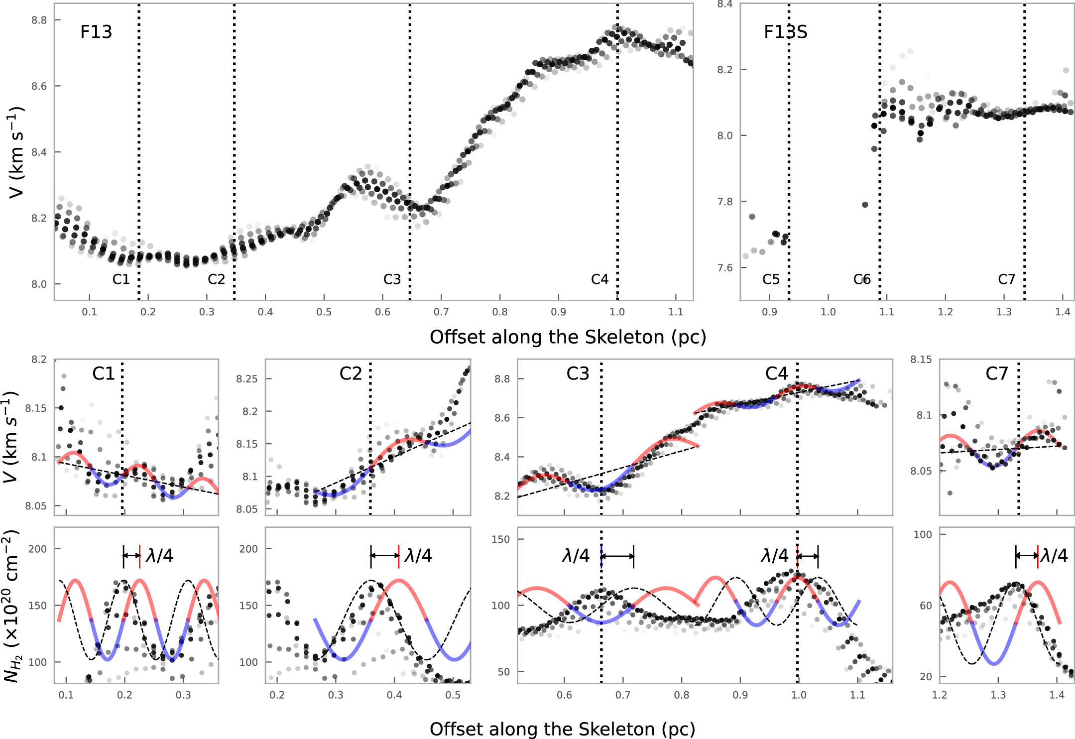
Figure 7. Longitudinal C18O (3 − 2) velocity (top and middle panels) and  variations (bottom panels) in F13 and F13S. The cores’ positions are presented with dotted vertical lines. Top: the longitudinal velocity variations along the crest, from south to north for F13 and from east to west for F13S. Only pixels located within a distance <0.05 pc from the crest are considered. Middle: same as in the top panels, but shown around each core. The curves depicted with red and blue are the best fit of the sinusoid to the radial velocity field and the dashed lines are the linear velocity gradients of the sinusoidal fits. Bottom: the longitudinal H2 column density variations, as shown in Figure 3, but around each core. The colored curve indicates the sinusoidal fit result in the middle panel, and its λ/4 shift is presented with the black dashed curve.
Download figure:
Standard image High-resolution imageA sinusoidal velocity distribution along the filament’s skeleton has been reported in previous molecular line studies (e.g., Hacar & Tafalla 2011; Chung et al. 2019, 2021; Kim et al. 2022; Shimajiri et al. 2023). It is explained as the result of core formation via fragmentation of the filament, and the oscillatory fluctuations of velocity and density are expected to present a shift of λ/4, where λ is the wavelength of both the density and velocity fluctuations (Hacar & Tafalla 2011; Kim et al. 2022; Shimajiri et al. 2023).
The middle and bottom panels in Figure 7 show the detailed longitudinal velocity and H2 column density profiles around the cores. We fitted a sinusoid function to the velocity profile and overlaid it with the red and blue curves. The λ/4-shifted curve is depicted with a dashed line on the  profile in the bottom panel. We found the best-fit sinusoid for C1, C2, and C7, where the position of the density peak is shifted by λ/4 from the velocity peak position. The observed velocity structures around the three cores agree with those of the core forming mass flow by filament fragmentation.
The sinusoidal variation for the other four cores was not clearly identified, as there were not enough C18O velocity data points for C5 and C6. C3 and C4 have the density peak position at the velocity minimum or maximum position. C3 and C4 have lower H2 column densities than C1 and C2, but the line masses Mline near C3 and C4 are larger than the critical line mass (see Figure 3 and Table 1). Hence, we can assume that the observed velocity fields around these two cores are also due to the mass inflow into cores along the filament, and we can infer the three-dimensional structure of the filament. Specifically, to have a minimum or maximum velocity at the density peak, F13 must possess a bend along the line of sight, where the high-velocity regions are located closer, and the low-velocity regions are situated farther away from us.
Figure 8 shows the velocity fields of F13 and F13S using 13CO (3 − 2) data, which were simultaneously obtained with the HARP observations of C18O (3 − 2) line. In a previous molecular line study toward this region, we found that the 13CO (1 − 0) emission is well matched with the Herschel 250 μm emission, while the C18O (1 − 0) emission is distributed only in relatively compact regions of high density (Chung et al. 2021). The 3 − 2 transitions of C18O and 13CO show similar emission distributions to their 1 − 0 transitions, and they are useful to trace dense filament regions and their diffuse envelope regions, respectively. Hence, we used the 13CO (3 − 2) emission to investigate the velocity fields covering diffuse gas over a larger area than the C18O (3 − 2) emission traces.
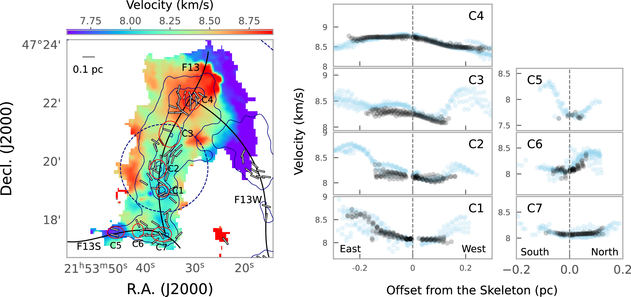
Figure 8. Velocity field map traced by the 13CO (3 − 2) molecular line data (left panel) and the radial velocity profiles centered on the cores are presented (right panels). Left: the 13CO(3 − 2) central velocity map derived by fitting the Gaussian function to the 13CO line profiles is displayed. Contour levels of H2 column density are presented at 30, 70, 110, and 150 × 1020 cm−2. The white segments represent the magnetic field vectors and the navy contours represent the Herschel column density. Right: presented are the transverse velocity profiles at each core’s position from east to west for F13 and from south to north for F13S. The black and sky-blue circles indicate the velocities traced from the C18O and 13CO (3 − 2) molecular lines, respectively.
Download figure:
Standard image High-resolution imageWe checked the 13CO (3 − 2) spectra and found that most line profiles over the region have a single Gaussian shape, but that profiles near C5 (the easternmost core of F13S) and the northern part of C4 (the northernmost core of F13) present double peaks. Hence, we performed a single Gaussian fitting for each line profile over most of the region, but a double Gaussian fitting for the spectra showing double peaks near C5 and the northern part of C4. We selected the higher velocity component between the two fitted components at the northern part of C4 and the lower velocity component near C5, which are similar to the velocity field of F13 and F13S, respectively. The central velocity map of 13CO (3 − 2) is displayed in the left panel of Figure 8, revealing a velocity field covering a broader region compared to C18O (3 − 2). In particular, in the northwest region, we can observe a low-velocity filament that was not detected in C18O. For F13, we can confirm the well-defined north–south velocity gradient seen in C18O as well as velocity gradients perpendicular to the major axis of the filament.
The transverse velocity fields at the positions of the cores are displayed in the right panels of Figure 8. The C18O emission is observed at small r (distance from the skeleton) and shows velocity gradients of ≲1 km s−1 pc−1. The 13CO data trace the velocity structure at larger r compared to the C18O data, and it is quite intriguing that they show that the velocity decreases as r decreases in all cores except for C4 core. The transverse velocity gradients range from about 1–5 km s−1 pc−1. This is quite larger than the velocity gradient along the major axis of the filament, but similar to the transverse velocity gradient shown in the B211 filament of Taurus (∼2 km s−1 pc−1; Palmeirim et al. 2013). The V-shape (or Λ-shape) transverse velocity structures have been observed in several filaments, which is explained as the result of the ongoing compression due to the propagating shock fronts (e.g., Arzoumanian et al. 2018; Bonne et al. 2020; Arzoumanian et al. 2022).
We calculated the nonthermal velocity dispersion (σNT) by extracting the thermal velocity dispersion (σT) from the observed total velocity dispersion (σobs):

where the observed total velocity dispersion was taken from the Gaussian fitting result. The thermal velocity dispersion of the observed molecule is

where kB is the the Boltzmann constant, T is the gas temperature, μobs is the atomic weight of the observed molecule (30 for C18O and 29 for 13CO), and mH the hydrogen mass, respectively. We used the dust temperature obtained from Herschel continuum data for the gas temperature (Arzoumanian et al. 2011). The resulting σNT is in a range of about 0.2–0.5 km s−1 with a mean value of 0.29 ± 0.06 km s−1.
The nonthermal velocity dispersion (σNT) of 13CO and C18O in units of the sound speed (cs
) are presented in Figure 9. The nonthermal velocity dispersion of 13CO and C18O are transonic to supersonic (cs
≲ σNT ∼ 2cs
) and subsonic to transonic (0.5cs
≲ σNT ≲ 1.5cs
), respectively. There is no increase in nonthermal velocity dispersion in specific regions of the filament, and there is no correlation with the column density. Rather, it can be seen that σNT of 13CO is about 1.5 times σNT of C18O. This larger σNT of 13CO can be caused by its larger optical depth than that of C18O. In addition, 13CO has a lower critical density than C18O, allowing it to trace regions with lower densities. Indeed, the width of 13CO in the spatial distribution is about twice that of C18O, and assuming that their depths in the line of sight are equal to their widths, σNT of 13CO will be about  times σNT of C18O. Thus, the constant ratio of nonthermal velocity dispersions between 13CO and C18O appears to be attributed to these distribution differences.
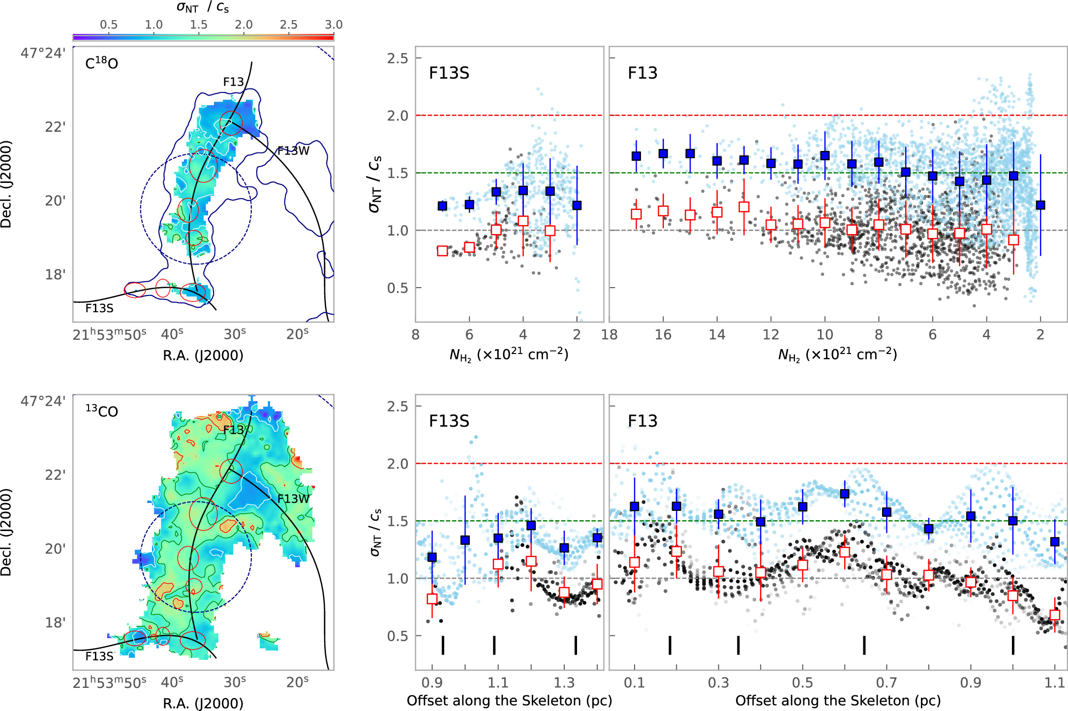
Figure 9. The distribution of nonthermal velocity dispersion normalized with the sound speed (σNT/cs). Left: the maps of σNT/cs from the C18O (top) and 13CO line profiles (bottom). The white, green, and red contours are σNT/cs = 1, 1.5, and 2, respectively. The navy contour on the σNT/cs map from the C18O is the 30 × 1020 cm−2 level of Herschel H2 column density. Right: σNT/cs as a function of H2 column density (top) and the distance along the skeleton from east to west for F13S and from south to north for F13 (bottom). σNT/cs from C18O and 13CO are illustrated with black and sky-blue colors, respectively, and their averaged values are presented with white and blue squares. The horizontal dashed lines indicate σNT/cs equals 1, 1.5, and 2. The positions of dense cores are denoted with black vertical lines in the bottom panels.
Download figure:
Standard image High-resolution image4. Analysis
4.1. Magnetic Field
4.1.1. Magnetic Field Geometry
Figure 10 illustrates the magnetic field orientations in the region. The large green segment is the large-scale magnetic field orientation obtained from the Planck 353 GHz polarization data.
10
We averaged the Q and U intensities over the F13 and F13S regions of  and measured the PA, and deduced the magnetic field angle by rotating the PA by 90°. The Planck data show that the averaged magnetic field over the filament is parallel to the main direction of F13. We note here that the size of F13 is quite smaller than the FWHM size of Planck observation (
 at 353 GHz; Planck Collaboration et al. 2016).
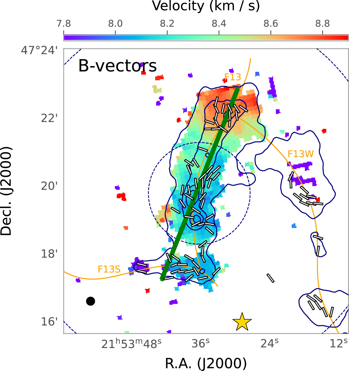
Figure 10. Magnetic field orientations on the C18O (3 − 2) moment 1 map. The navy contours are the Herschel column density of 30, 70, 110, and 150 × 1020 cm−2. The selection criteria for magnetic field vectors are the same as in Figure 4. All the B-field segments are shown with equal lengths to better display the B-field orientation. The green segment displays the large-scale B-field orientation deduced from the Planck 353 GHz polarization vector. The yellow star at the south and the black circle at the bottom left corner represent the position of BD+46 and the POL-2 850 μm beam size of 141, respectively.
Download figure:
Standard image High-resolution imageThe core-scale magnetic field vectors inferred by rotating the 850 μm polarization vectors by 90° are presented with white segments in Figure 10. The magnetic field vectors in F13S align mostly parallel to the directions of the filament’s skeleton. However, in F13, the magnetic field orientations appear to be more complex. At the northern and western parts of F13, the magnetic field vectors tend to align parallel to the direction of the filament’s skeleton. Conversely, perpendicular B-field vectors are observed in the southern and eastern parts. In Figure 11, the position angle distribution of B-field vectors is presented. The B-field angle distribution of F13 peaks at about 45° and 165°, the former attributed to the vectors near C1, while the latter is close to the mean field orientation observed with Planck. The histogram of the B-field orientation of F13S peaks at ∼105°, which is consistent with the main direction of F13S.
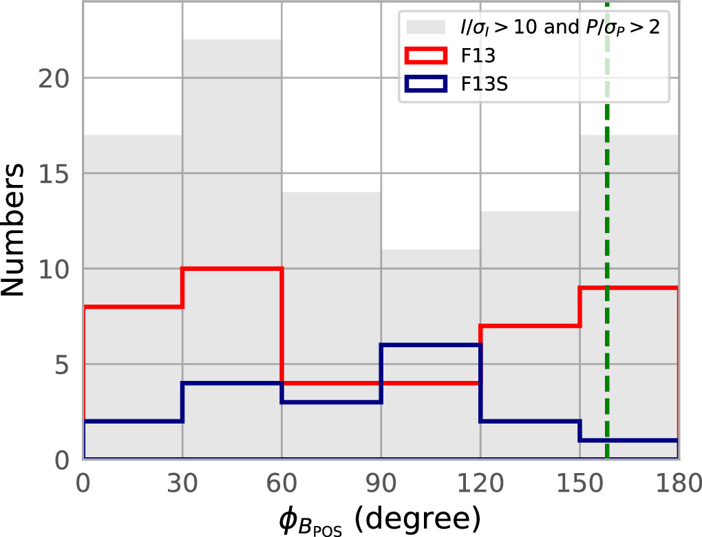
Figure 11. Histogram of the position angles for the magnetic field orientations presented in Figure 10. The filled histogram is for all the B-field vectors with I/σI > 10 and P/σP > 2 over the observed region, and the red and navy histograms are for those in F13 and F13S, respectively. The green dashed line indicates the Planck B-field orientation (see the green segment in Figure 10).
Download figure:
Standard image High-resolution imageThe magnetic field orientation with respect to the filament axis has been reported to change in a way that B fields are aligned parallel to the filament at low column density, but become perpendicular at high column density of  (e.g., Planck Collaboration et al. 2016). In the case of F13S,
  is ≲70 × 1020 cm−2.
  range of F13 is much larger than that of F13S up to ∼170 × 1020 cm−2. And the magnetic field geometry is likely to be disordered at the high-density regions of ≳110 × 1020 cm−2.
F13S shows an increase in velocity along the east–west direction, which coincides with the filament’s skeleton direction (see Figures 7 and 8). The magnetic field direction also aligns with this trend of the velocity field. F13 also shows an increment in velocity from south to north, aligned to the main direction. At the southern region of F13, near C1, a decrement in velocity is found from east to west (see the transverse velocity profile of C1 in Figure 8). The B-field orientations in the region tend to align east–west direction, which is close to the transverse velocity gradient. However, due to the low S/N of the polarization vectors, we would like to tread cautiously in interpreting these results.
4.1.2. Magnetic Field Strength
We estimated the magnetic field strength using the modified Davis–Chandrasekhar–Fermi (DCF) method (Davis 1951; Chandrasekhar & Fermi 1953a). The DCF method assumes that the underlying magnetic field is uniform but distorted by the turbulence, and calculates the strength of the magnetic field in the molecular clouds using the angular dispersion of the magnetic field vectors (δ ϕ), velocity dispersion (σ), and number density of the gas (ρ) with the following equation (Crutcher et al. 2004):

where Qc is the correction factor for the overestimation of the magnetic field strength due to the beam integration effect. Qc of 0.5 was adopted from Ostriker et al. (2001).  is the number density of the molecular hydrogen per cubic centimeter, and
  in kilometers per second.
The mean H2 volume density along the crest ( ) and Δv measured from the nonthermal velocity dispersion given in Table 1 were used.
To estimate the angular dispersion of magnetic field vectors (δ ϕ), we adopted two independent methods. One is the unsharp-masking method (Pattle et al. 2017) and the other is the structure function (Hildebrand et al. 2009). The unsharp-masking method measures the angular dispersion of the magnetic field distorted by the turbulence motions by removing the underlying magnetic field geometry (Pattle et al. 2017). To obtain the large-scale background magnetic field structure, the observed magnetic field map is smoothed with an n × n pixel boxcar filter, where n is an odd number. After obtaining the large-scale background magnetic field structure, the smoothed map is subtracted from the original map. Finally, the angular dispersion is measured from the residual map. We applied a 3 × 3 pixel boxcar filter to the observed magnetic field map.
Figure 12 shows the position angle map of the observed magnetic field vectors (left), smoothed PA map (middle), and the residual map (right). To avoid underestimating δ
ϕ due to the nondetected pixels and the small number of pixels in the boxcar filter, we used the residual values only when the number of data points in the 3 × 3 boxcar filter is at least five in the calculation of δ
ϕ. The obtained angular dispersions are δ
ϕ = 91 ± 2
4 and 16
0 ± 2
6 for F13 and F13S, respectively.
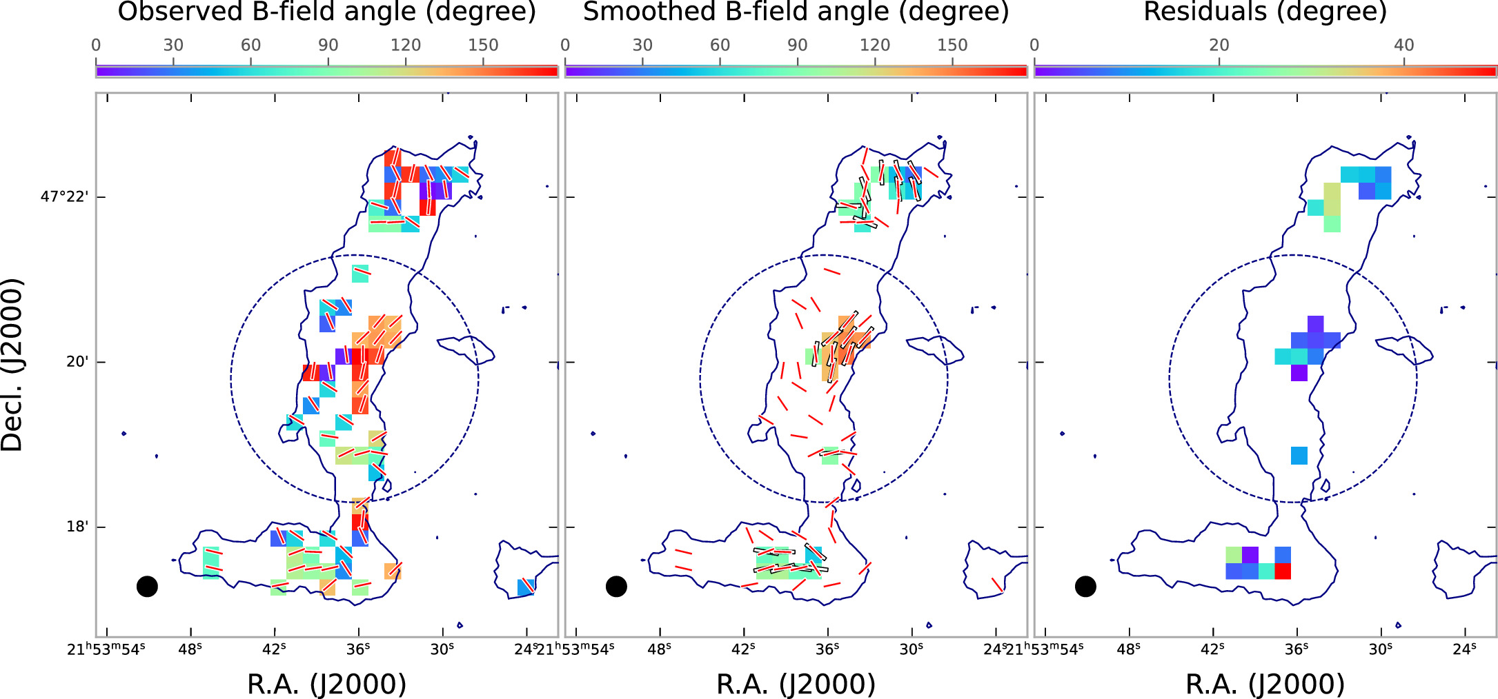
Figure 12. The magnetic field angle maps of the observed (left), smoothed (center), and residual (right). The orientations of the observed magnetic field vectors are drawn with red bars in the left and central panels and the smoothed B-field vectors are presented with white bars in the central panel. The data of smoothed and residual maps are shown only if the number of selected B-field vectors within a 3 × 3 box is ≥5. The dashed and solid circles indicate the  central region and 14
1 JCMT beam size at 850 μm.
Download figure:
Standard image High-resolution imageThe second method we have used to determine the angular dispersion of the magnetic field vectors is the structure-function model, which is “designed to avoid inaccurate estimates of turbulent dispersion due to a large-scale, nonturbulent field structure” (Hildebrand et al. 2009). In the model, the structure function of the angle difference in a map is calculated as the following equation:

where Φ(x) and ΔΦ(l) ≡ Φ(x) − Φ(x + l) are the angle at the position x and the angle difference between the vectors with separation l. N(l) is the number of pairs of the vectors. The magnetic field is considered to consist of two components: a large-scale magnetic field and a turbulence-scale magnetic field affected by the turbulence. As the scale l increases within the range 0 ≤ l ≪ d, where d is the scale of the large-scale structured magnetic field, the contribution of the large-scale magnetic field to the dispersion function is expected to increase nearly linearly. The impact of turbulence on the magnetic fields can be described as follows: (1) At very small scales (l → 0), the effect of turbulence is almost negligible or close to zero, (2) the turbulence has the most significant influence at scales approximately equal to the turbulent scale (δ), and (3) for scales larger than the turbulent scale (l > δ), the effect of turbulence remains constant. Then, the Equation (16) can be presented as follows (Hildebrand et al. 2009):

where 〈ΔΦ2(l)〉tot is the square of the total measured dispersion function. The term b represents the constant turbulent contribution to the angular dispersion within the range δ < l < d. The parameter m characterizes the linearly increasing contribution of the large-scale magnetic field.  accounts for the correction term due to the measurement uncertainty when dealing with real data.
Figure 13 illustrates the square root of corrected angular dispersion ( ) as a function of distance l. The data have been divided into distance bins with separations corresponding to the pixel size of 12″. We performed best-fit analyses using the first three data points to ensure that the condition l ≪ d is satisfied. The parameter b2 was obtained from the least square fitting of the relation, resulting in estimated values of b for F13 and F13S as 17.0 and 18.5, respectively. The corresponding angular dispersions
  to be applied to the modified DCF method are 12
0 ± 6
2 and 13
1 ± 2
1 for F13 and F13S, respectively.
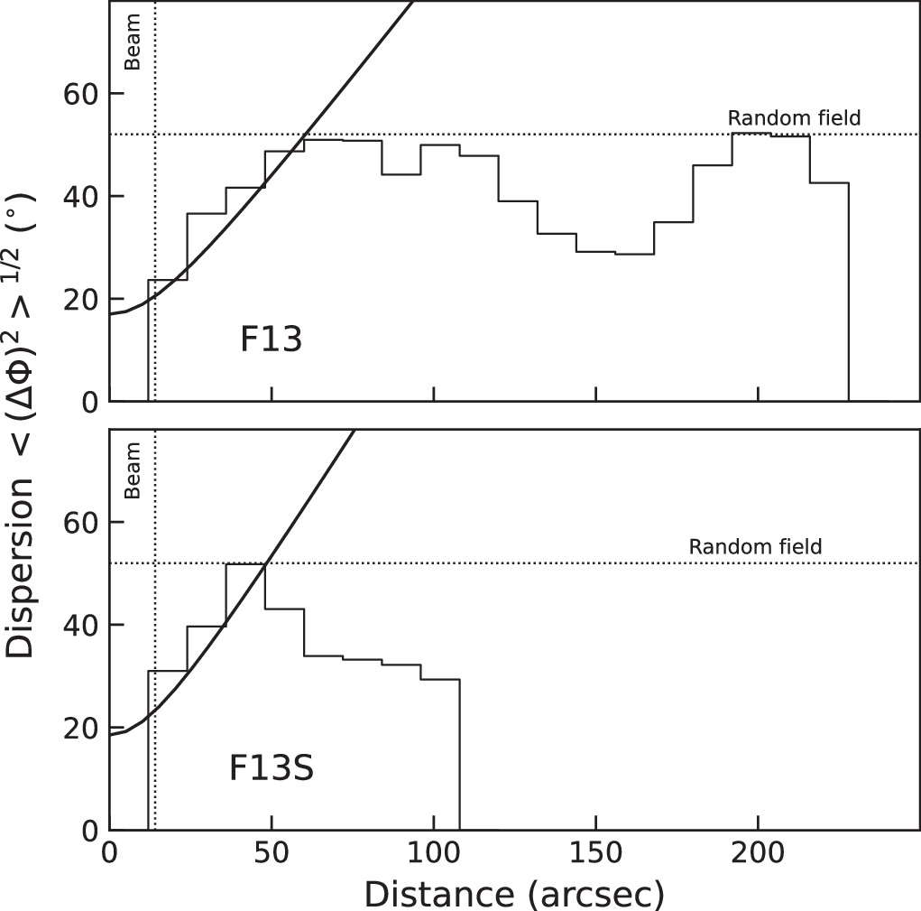
Figure 13. The angular dispersion function ( ) is shown for F13 (top) and F13S (bottom). The solid thick curve represents the best-fit model. The intercept of the fit at the zero-point determines the contribution of turbulence to the total angular dispersion. The vertical dotted line indicates the beam size of POL-2 at the 850 μm wavelength, which is 14
1. The horizontal dotted line represents the expected
 for a random field, which is 52°.
Download figure:
Standard image High-resolution imageTable 3 presents the applied  , Δv, δ
ϕ, and measured magnetic field strengths for F13 and F13S. The magnetic field strengths derived from the unsharp-masking method are 76 ± 23 and 33 ± 7 μG for F13 and F13S, respectively. Using the structure function method, the estimated magnetic field strengths are 58 ± 31 and 40 ± 9 μG for F13 and F13S, respectively. It is important to note that the values of BPOS obtained from both methods agree well with each other within the uncertainties involved. Hereafter, we will denote quantities obtained using the unsharp-masking method with the superscript UM and those from the structure-function method with the superscript SF.
, Δv, δ
ϕ, and measured magnetic field strengths for F13 and F13S. The magnetic field strengths derived from the unsharp-masking method are 76 ± 23 and 33 ± 7 μG for F13 and F13S, respectively. Using the structure function method, the estimated magnetic field strengths are 58 ± 31 and 40 ± 9 μG for F13 and F13S, respectively. It is important to note that the values of BPOS obtained from both methods agree well with each other within the uncertainties involved. Hereafter, we will denote quantities obtained using the unsharp-masking method with the superscript UM and those from the structure-function method with the superscript SF.
Table 3. Magnetic Field Strengths and Energies
| F13 | F13S | |||
|---|---|---|---|---|
 (103 cm−3) (103 cm−3) | 11.0 ± 2.4 | 7.0 ± 0.7 | ||
| Δv (km s−1) | 0.72 ± 0.08 | 0.68 ± 0.11 | ||
| Unsharp masking | Structure function | Unsharp masking | Structure function | |
| δ ϕ (deg) | 9.1 ± 2.4 | 12.0 ± 6.2 | 16.0 ± 2.6 | 13.1 ± 2.1 |
| Bpos (μG) | 76 ± 23 | 58 ± 31 | 33 ± 7 | 40 ± 9 |
| λ | 0.31 ± 0.13 | 0.40 ± 0.25 | 0.32 ± 0.12 | 0.26 ± 0.10 |
| VA (km s−1) | 1.22 ± 0.37 | 0.92 ± 0.50 | 0.66 ± 0.16 | 0.80 ± 0.19 |
| MA | 0.25 ± 0.08 | 0.33 ± 0.18 | 0.44 ± 0.13 | 0.36 ± 0.10 |
| EB (M⊙ km2 s−2) | 56.4 ± 26.9 | 32.3 ± 21.1 | 2.6 ± 1.1 | 3.9 ± 1.6 |
| EG (M⊙ km2 s−2) | 22.0 ± 16.1 | 1.1 ± 0.8 | ||
| EK (M⊙ km2 s−2) | 12.3 ± 4.9 | 2.0 ± 0.8 | ||
Download table as: ASCIITypeset image
4.2. Magnetic Field, Gravity, and Turbulence
We estimated the mass-to-magnetic flux ratio (λ) and Alfvénic Mach number (MA) to investigate the significance of magnetic fields with respect to the gravity and turbulence.
The mass-to-magnetic flux ratio (λobs) is presented as

where  and
and  are the observed and the critical mass-to-magnetic flux ratios, respectively.
  is calculated with the following equation:

where  and
and  are the mean molecular weight per hydrogen molecule of 2.8 and the H2 column density. The critical mass-to-magnetic flux ratio is
  (Nakano & Nakamura 1978). Equation (18) can be expressed following Crutcher et al. (2004) as

The mean H2 column density on the crest ( ) was used for
  . The actual λ value is assumed to be λobs/3 considering the statistical correction factor of 3 for the random inclination of the filament (Crutcher et al. 2004). The criterion for the significance of magnetic fields is given in a way that if λ is less than 1, then magnetic fields are expected to support the clouds, while λ greater than 1 would mean the structure is in a gravitational collapse.
For F13 and F13S, the values of λUM are 0.31 ± 0.13 and 0.27 ± 0.09, respectively. When using the structure function method, the corresponding values are λSF of 0.41 ± 0.25 and 0.22 ± 0.08, respectively. These results suggest that both F13 and F13S are likely supported by magnetic fields, as their λ values are less than 1.
We estimated the Alfvénic Mach number (MA) by

where σNT and VA are the nonthermal velocity dispersion and the Alfvén velocity, respectively. VA is defined as  where B and
  are the total magnetic field strength and the mean density, respectively. The statistical average value of Bpos, (4/π)Bpos, was used for B (Crutcher et al. 2004), and the mean density was obtained from
  . F13 and F13S have
  of 1.21 ± 0.36 and 0.79 ± 0.16 km s−1 and
  of 0.91 ± 0.49 and 0.97 ± 0.20 km s−1, respectively. The Alfvénic Mach numbers of the two filaments are less than 0.5, and hence, F13 and F13S are both sub-Alfvénic, indicating the magnetic fields dominate turbulence in the regions.
We calculated the total gravitational (EG), kinematic (EK), and magnetic field energies (EB) assuming the cylindrical geometry of F13 and F13S using the following equations (Fiege & Pudritz 2000):


and

where M and L are the mass and length of filament, respectively. σtot is the total velocity dispersion estimated by the equation,

where μp = 2.37 is the molecular weight of the mean free particle (Kauffmann et al. 2008).
The estimated quantities are tabulated in Table 3. F13 exhibits significantly larger EG, EK, and EB, approximately 5–20 times greater than F13S. This difference can be attributed to F13's larger mass compared to F13S. In Figure 14, the relative energy distributions are represented using donut diagrams, where  is employed to denote the energy portions. As depicted in the Figure, the largest energy contribution for both F13 and F13S comes from the magnetic field (≳50%). The energy distributions of the two filaments that have the largest portion in the magnetic field energy agree with those of filaments that have quasiperiodically aligned dense cores (Chung et al. 2023). Meanwhile, the portions of magnetic field energy in F13 and F13S are quite larger than those in the E- and W-hubs of the dark Streamer of IC 5146 (EB ∼ 20%; Chung et al. 2022). While the comparison is limited to a few filaments, this supports the proposal by Chung et al. (2021) that, in the filaments of the Cocoon Nebula, thermal pressure and magnetic fields may be more crucial than turbulence compared to the filaments in the dark Streamer.
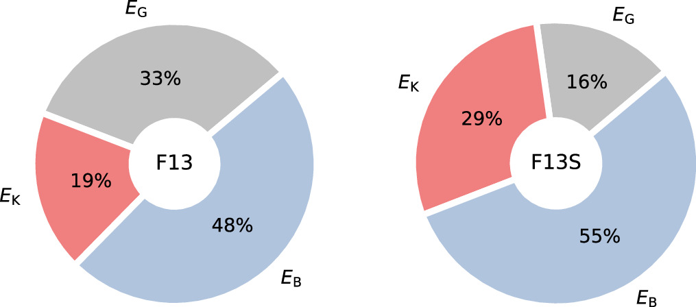
Figure 14. Respective energy components, including gravitational energy (EG), kinematic energy (EK), and magnetic energy ( ) are depicted for F13 (left) and F13S (right) with their relative proportions represented by distinct colors: gray for EG, red for EK, and blue for
  . The values indicate the occupying percentage of each energy component.
Download figure:
Standard image High-resolution image4.3. B-field Distributions
We obtained the distribution of magnetic field strengths by applying the modified DCF method on a pixel-by-pixel scale (e.g., Hwang et al. 2021). A δ
ϕ map was obtained using the residual map of magnetic field angles in Figure 12. If the number of angle residuals within a 3 × 3 box is ≥3, the standard deviation of residual PAs was measured for δ
ϕ. An H2 number density map was estimated with Equation (2) and a Δv map was made from the calculation of the nonthermal velocity dispersion as  . The distribution maps of
  , Δv, and Δϕ are presented in Figure 15. Due to the nondetected pixels mostly in dense regions, we have a total of 24 detected pixels in the map.
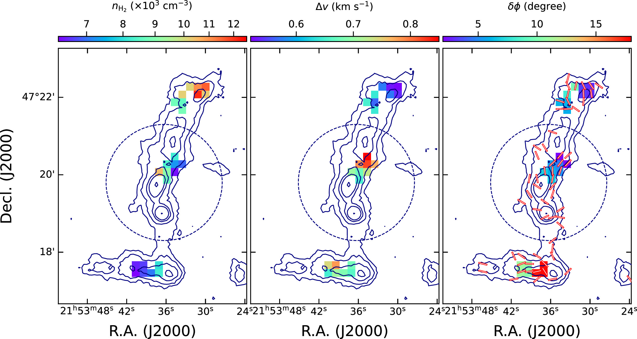
Figure 15. The spatial distributions of  , Δv, and δ
ϕ with the 850 μm emission contours. The data is shown only if δ
ϕ is measured where the number of angle residual data points within a 3 × 3 box is ≥3. The observed magnetic field vectors with I/σI
≥ 10 and P/σP ≥ 2 are drawn in the δ
ϕ map.
, Δv, and δ
ϕ with the 850 μm emission contours. The data is shown only if δ
ϕ is measured where the number of angle residual data points within a 3 × 3 box is ≥3. The observed magnetic field vectors with I/σI
≥ 10 and P/σP ≥ 2 are drawn in the δ
ϕ map.
Download figure:
Standard image High-resolution imageThe spatial distribution of Bpos was obtained by using the  , Δv, and Δϕ distributions and is shown in Figure 16 with the mass-to-magnetic flux ratio map and the Alfvénic Mach number map obtained with Equations (20) and (21). The magnetic field strength mostly ranges from ∼30–200 μG. The λ and MA
distributions show that the ranges are both between 0.2 and 0.5, indicating that the regions are magnetically subcritical and sub-Alfvénic throughout. However, although there are almost no data points in the high-density region, higher-density regions tend to exhibit a higher mass-to-magnetic flux ratio, particularly in the directions toward two dense cores, C2 and C7. Hence, we do not rule out the possibility that the dense regions are magnetically supercritical, given that the uncertainties in λ are large.
, Δv, and Δϕ distributions and is shown in Figure 16 with the mass-to-magnetic flux ratio map and the Alfvénic Mach number map obtained with Equations (20) and (21). The magnetic field strength mostly ranges from ∼30–200 μG. The λ and MA
distributions show that the ranges are both between 0.2 and 0.5, indicating that the regions are magnetically subcritical and sub-Alfvénic throughout. However, although there are almost no data points in the high-density region, higher-density regions tend to exhibit a higher mass-to-magnetic flux ratio, particularly in the directions toward two dense cores, C2 and C7. Hence, we do not rule out the possibility that the dense regions are magnetically supercritical, given that the uncertainties in λ are large.
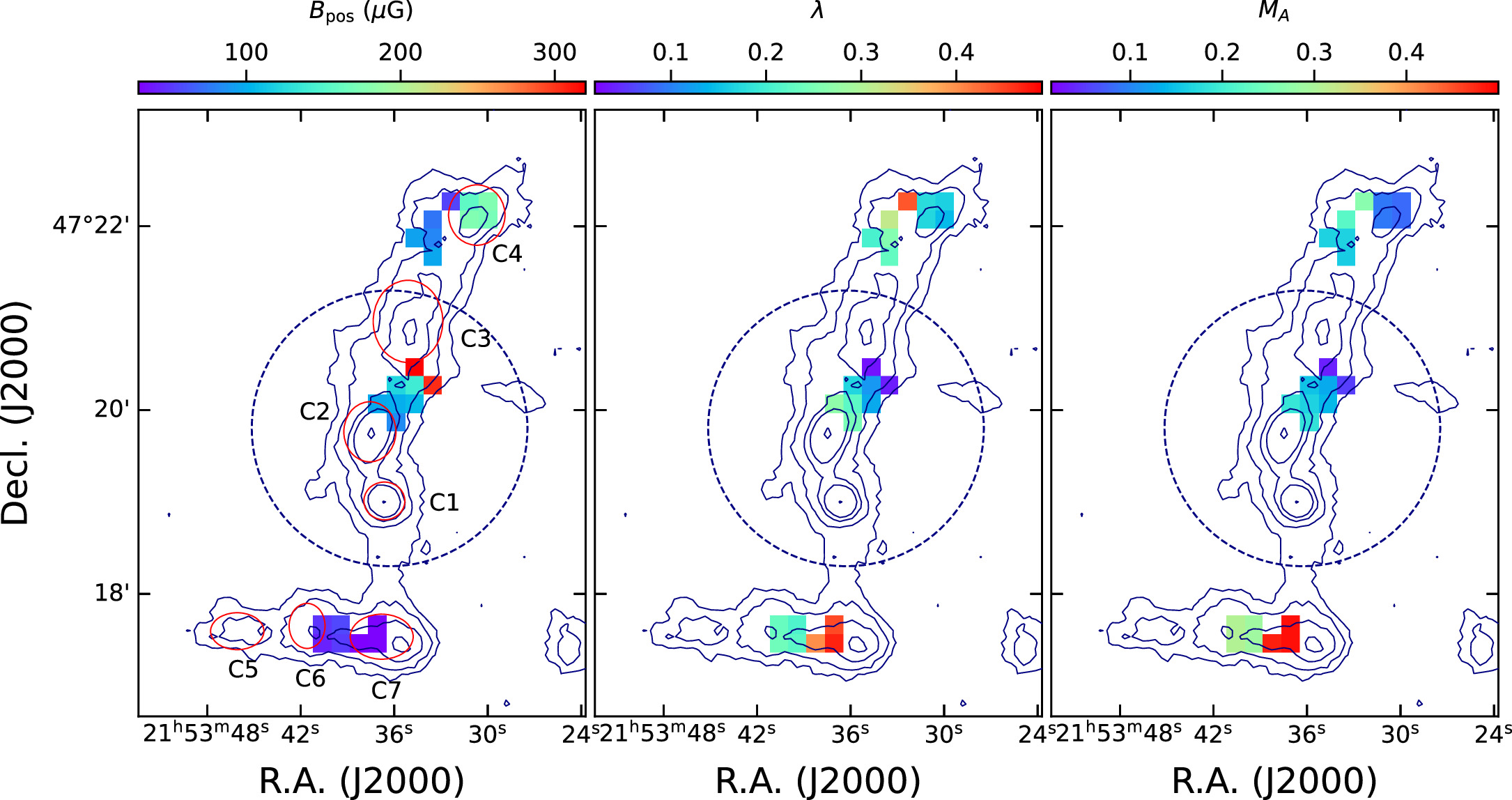
Figure 16. The spatial distributions of BPOS, λ, and MA with the 850 μm emission contours. The red ellipses in the BPOS map present the dense cores.
Download figure:
Standard image High-resolution image5. Discussion
The basic picture of the Cocoon Nebula given by the H i observations is a blister H ii region formed by a B0 V single star BD+46 in front of the parent molecular cloud (Roger & Irwin 1982). It is reported that the maximum radius of H ii region is 1.2 pc (Roger & Irwin 1982) and the H i to H2 transition is occurred at the distance of 1.44 pc from BD+46 (Aannestad & Emery 2003) assuming the distance of 813 pc to the Cocoon Nebula. F13 and F13S are located behind the H ii region formed by BD+46 (Roger & Irwin 1982). Figure 17 presents the Herschel column density map with an imaginary three-dimensional sphere. The skeletons of filaments in the region are overlaid, and the redshifted (vlsr ∼ 8.0–8.9 km s−1) and blueshifted (vlsr ∼ 7.0–8.4 km s−1) 13CO emissions are represented with red and blue contours. The H ii region and the H i to H2 transition region are depicted with the white dashed circle and solid sphere in Figure 17, respectively. As shown in the Figure, F13 and F13S likely reside on the imaginary sphere with a radius of 1.44 pc. In this section, we will discuss the dust polarization properties, filament formation, and core formation using this picture of Cocoon Nebula.
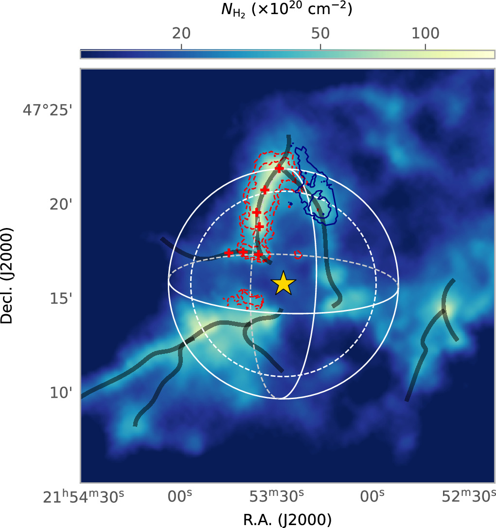
Figure 17. Imaginary picture of the Cocoon Nebula system. The H2 column density map from Herschel is presented, and the filaments’ skeletons are overlaid with thick black curves (Arzoumanian et al. 2011). The positions of dense cores and BD+46 are displayed with red crosses and a big yellow star, respectively. The blue and red 13CO components integrated over the velocity ranges of 7–8.4 and 8–8.9 km s−1, respectively, are illustrated with solid navy and dotted red lines. The imaginary three-dimensional sphere with a radius of 01 (identical to 1.44 pc at the assumed distance of 813 pc) is shown in white color. The white dashed circle indicates the size of H ii region (radius of 1.2 pc at the distance of 813 pc; Roger & Irwin 1982).
Download figure:
Standard image High-resolution image5.1. The Radiation Field of BD+46 and the Dust Polarization Fraction
Ngoc et al. (2021) found that the California LkHα 101 region surrounding an early B star, LkHα 101, has a single power-law slope of α = 0.82 ± 0.03. They interpreted the rapid decrease in P as I increases as due to the mixing effect of the magnetic field tangling and grain alignment with rotational disruption by radiative torques. In the south of F13S, there is a B0 V single star, BD+46. α of the single power-law fit over the F13 region is 0.82 ± 0.09 estimated with the vectors of I/σI ≥ 10 and P/σP ≥ 3, and it is quite similar value to that of LkHα 101.
To examine whether the α of F13 region is related to the radiation field of BD+46, we divided the filament into two near and far regions from BD+46 with respect to the skeleton of the filaments. We applied the Ricean-mean model to those vectors of the near and far regions separately. In Figure 5, the vectors of the near and far regions are colored with red and blue, respectively, and their best-fit results are drawn with the same color code. In Table 2, the best-fit results are tabulated. Shown is that the vectors of the near region to BD+46 have a slightly steeper slope (α = 0.73 ± 0.07) than the vectors in the far region have (α = 0.71 ± 0.13). However, the difference between them is smaller than their uncertainties.
Figure 18 presents the polarization fraction (P) plotted against the projected distance from BD+46. No significant correlation between distance and P is observed. However, for distances smaller than 160″, the closer vectors show a larger mean P compared to the far vectors. This could serve as indirect evidence that the radiation field of BD+46 influences the dust alignment efficiency in the region, and consequently, the polarization fraction. It is crucial to note that there is only one far vector in the bin between 80″ < r ≤ 120″, and thus, we cannot rule out the possibility of bias due to the small sample size. Above all, if F13 and F13S are indeed located on the surface of a sphere with a radius of 1.44 pc, as depicted in Figure 17, it would provide a compelling explanation for the lack of correlation between the projected distance and the degree of polarization.
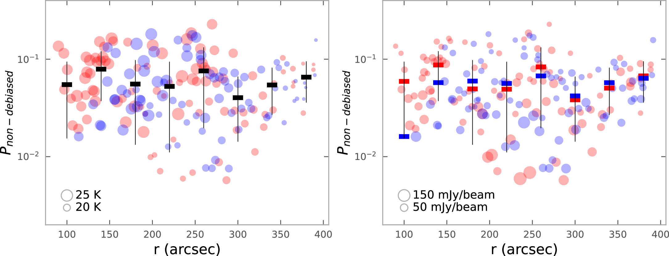
Figure 18. The polarization fraction as a function of distance from BD+46. The two panels show the same distribution with the marker sizes scaled by the dust temperature in the left panel and the Stokes I intensity in the right panel. The red and blue colors indicate the position of vectors in the filaments, i.e., the red and blue are for the vectors close to and far from BD+46. The black thick horizontal bar in the left panel is the average of non-debiased P in every 40″ bin, and the red and blue horizontal bars in the right panel are those for the vectors close to and far from BD+46, respectively.
Download figure:
Standard image High-resolution image5.2. Possible Formation of F13 by Radiation Shock Front of BD+46
Theoretically, filaments can form through self-gravitational fragmentation within a sheet-like cloud created by shock compression (e.g., Tomisaka & Ikeuchi 1983; Nagai et al. 1998). This compression is induced by feedback from massive stars, cloud–cloud collisions, and galactic spiral shocks, as well as from expanding H ii regions. In a filament formed through shock compression within a sheet-like cloud, a notable characteristic is the V-shape (or Λ-shape) transverse velocity structure, which is attributed to mass flows induced along magnetic field lines or by self-gravity (e.g., Arzoumanian et al. 2018; Inoue et al. 2018; Abe et al. 2021). In case the ordered magnetic field causes mass flow from the natal cloud and formation of filament, the major direction of the filament becomes perpendicular to the magnetic field direction (Inoue & Fukui 2013; Inoue et al. 2018). However, the large-scale magnetic field direction deduced from the Planck polarization data is almost parallel to the major direction of F13, and the high-resolution B-field vectors from the POL-2 polarization data are mostly longitudinal, too (see Figure 10). Thus, the velocity structure of F13 and F13S is not likely induced by the magnetic field lines.
When the initial magnetic field strength is smaller than 200 μG, a sheet compressed via the H ii region of a young OB star becomes unstable, leading to the formation of a dense filament (Tomisaka & Ikeuchi 1983). If the thickness of the layer is smaller than the pressure scale height, the major orientation of the filament aligns parallel to the magnetic field lines (Nagai et al. 1998). The measured magnetic field strength of F13 (≲140 μG; see Table 3 and Figure 16), along with the observed parallel magnetic field direction (Figure 10), suggests the possibility that it may have originated from a thin shock-compressed layer around the H ii region created by BD+46 with a weak magnetic field. Moreover, Abe et al. (2021) conducted isothermal magnetohydrodynamics simulations to explore filament formation, specifically examining the effects of shock velocity and turbulence. In the fast shock mode (with a shock velocity of ∼7 km s−1), they found that filaments form regardless of the presence of turbulence and self-gravity. Conversely, in the slow shock mode with a shock velocity of ∼2.5 km s−1 and low turbulence, self-gravity likely plays a more significant role. It is worth noting that Roger & Irwin (1982) reported an expanding velocity of ∼2.3 km s−1 for the H i gas in the Cocoon Nebula, with the ionization front on the far side moving at 2 km s−1. Consequently, it is presumed that F13 and F13S were formed in a low-shock environment, in which case self-gravity would have played a significant role.
Figure 19 shows the formation process of F13 schematically. The age of BD+46 is estimated to be approximately 2 Myr (García-Rojas et al. 2014), so it can be inferred that the shock wave originated from BD+46 around 2 Myr ago. Assuming a shock velocity of 2.3 km s−1 and a distance of 1.44 pc between BD+46 and F13, it would take 6 × 10⁵ yr for the shock to reach the parent molecular cloud of F13. The nonthermal velocity dispersion (σNT) is used as indirect evidence of the turbulent motion of gas induced by shocks, accompanied by velocity variations (e.g., Pineda et al. 2010; Kim et al. 2022). The gas in the region where the shock front reaches would become more turbulent and have larger σNT values. However, there is no apparent correlation between the nonthermal velocity dispersion and the radiation shock effects (Figure 9). The absence of any discernible impact from radiation shocks in the nonthermal velocity dispersion distribution is likely due to, as mentioned above, the radiation shock front passed through approximately 1.4 Myr ago.
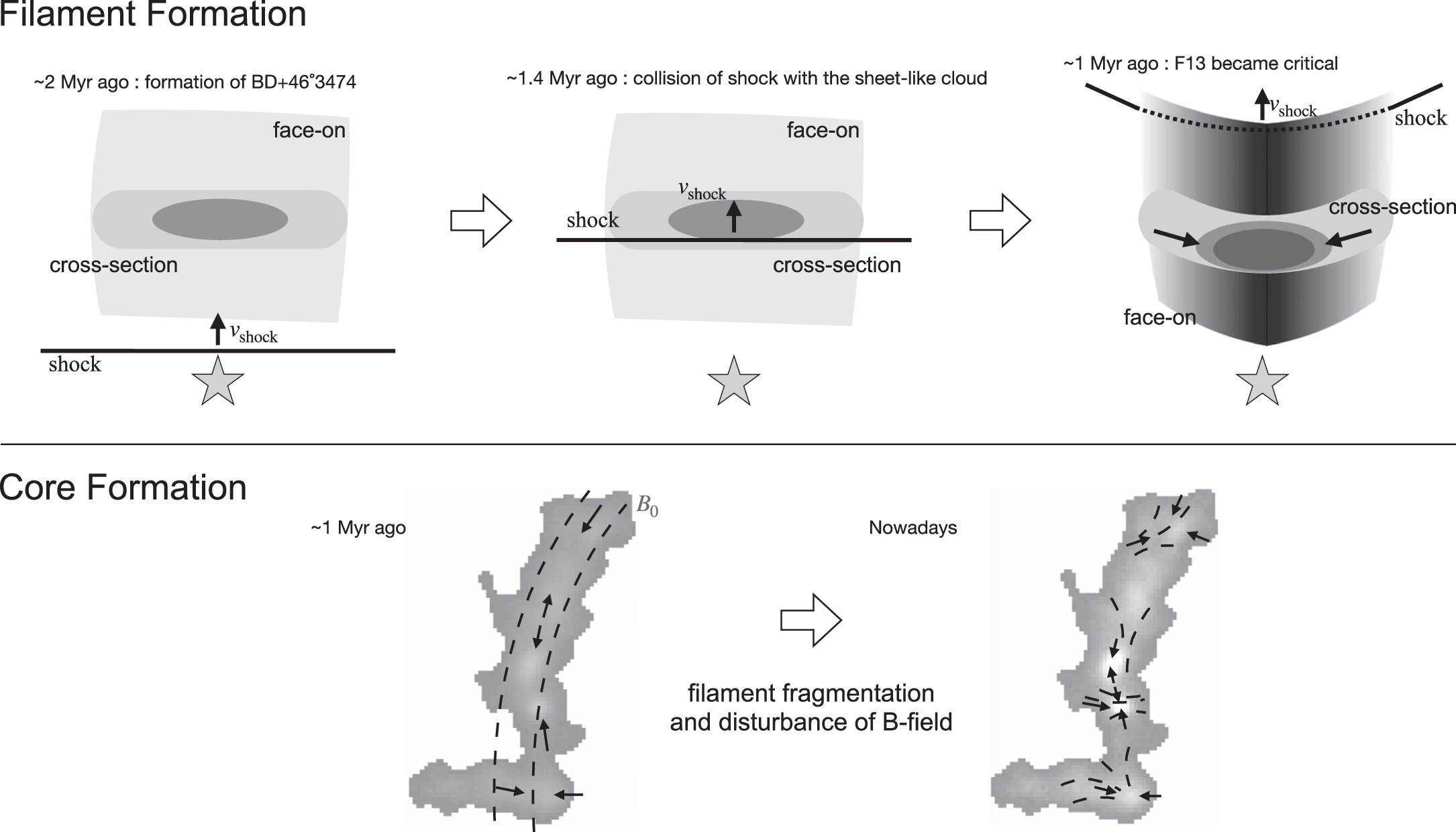
Figure 19. Schematic figure of the filament’s formation and evolution. Top: molecular cloud before and after the collision with the radiation shock front. The face-on view and cross-section of the molecular cloud are colored with a gray tone, while the dense filament formed through the collision is shaded in a deep tone. The direction of the shock front and the mass flow from the less dense ambient cloud to the dense filament are represented with arrows. Bottom: core formation by the filament fragmentation. The magnetic field and mass flow along the filament are presented with black dashed curves and arrows.
Download figure:
Standard image High-resolution imageThe shock wave might compress the sheet, causing the compressed region to become denser. Subsequently, condensation due to self-gravity would have occurred. The V-shaped velocity structure seen in Figure 8 could be attributed to the accretion of material that occurred during the formation process of F13. The transverse velocity differences at the filament crest and the radial distance of 0.2 pc of F13 (0.1 pc of F13S) as shown in Figure 8 are ∼0.2–0.7 km s−1 (∼0.1–0.5 km s−1 for F13S). Considering these transverse velocity differences, the infall velocity from the natal cloud,  , is expected to be 0.4 ± 0.1 and 0.3 ± 0.1 km s−1 for F13 and F13S, respectively. The mass accretion rate per unit length onto the filament (
 ) from the natal cloud can be measured with the following Equation (e.g., Palmeirim et al. 2013; Arzoumanian et al. 2022):

where ρ(R) is the density at the infall radius R (0.2 pc for F13 and 0.1 pc for F13S). ρ(R) is estimated to be  from the column density at R (2 × 1021 cm−2) divided by F13's width (0.32 pc), and the mean molecular weight of 2.8 is used. The measured mass accretion rate per unit length is ∼70 ± 30 M⊙ pc−1 Myr−1 for F13 and ∼30 ± 10 M⊙ pc−1 Myr−1 for F13S. Then, it would take 9 ± 5 × 10⁵ yr and 8 ± 4 × 10⁵ yr for F13 and F13S to have current mass per unit lengths of 67 and 22 M⊙ pc−1 at the current accretion rates. The thermal critical line masses of F13 and F13S are 27 and 33 M⊙ pc−1, respectively, and they may become critical in 4 ± 1 × 10⁵ yr for F13 and 12 ± 5 × 10⁵ yr for F13S. This suggests that since the formation of BD+46 occurred approximately 2 Myr ago, the radiation shock front collided with the sheet-like cloud around 1.4 Myr ago. F13 increased its line mass through infall mass driven by self-gravity, reaching a critical state around 1 Myr ago, potentially leading to the formation of dense cores. In the case of F13S, it became critical approximately 0.2 Myr ago. This indicates that a considerable period has elapsed since the formation of F13, enabling the formation of dense cores within the filament up to the present moment. In contrast, this has not been the case for F13S, possibly leading to less distinct fragmentation features due to a limited time for evolution.
5.3. Filament Fragmentation and Core Formation
After the formation of F13 and F13S through shock compression and mass infall due to self-gravity, it is likely that dense cores were generated through the fragmentation process. F13 and F13S have four and three dense cores, respectively, and the cores are well aligned on their parental filament’s crest. The mean projected separations of cores in F13 and F13S are 0.27 ± 0.08 and 0.20 ± 0.05 pc, respectively.
It is in broad agreement that the periodically aligned cores are the fragments of cylindrical filaments via gravitational instability, which was first proposed by Chandrasekhar & Fermi (1953b) and refined later in a few studies (see Section 4 of Jackson et al. 2010). The theoretical model assumes an isothermal, infinitely long cylindrical structure, and its fragmentation occurs through gravitational perturbations with critical wavelengths. Then, the filaments may possess cores with regular spacing, representing the fastest-growing mode of fragmentation. In the pressure-confined models where the isothermal cylinder with the external pressure by an ambient medium is assumed, the wavelength of the fastest-growing mode,  , is proposed to be ∼5 × the filament’s width (Nagasawa 1987; Fischera & Martin 2012). The mean core separations in F13 and F13S are similar to those of the filaments’ widths, and quite smaller than that expected by the model.
The disagreement between the theoretical prediction and observational core spacings could be caused by their different density profiles from that assumed in the theoretical model. Nagasawa (1987) stated the case in which the isothermal scale height ( ) of the filament is much smaller than the filament’s radius (H ≪ R). In this case,
  equals 22 × H. H estimated with the mean dust temperature and central density in Table 1 are 0.012 and 0.016 pc for F13 and F13S, respectively, and their radii are larger than ∼14 and 7 times the isothermal scale heights, respectively. Thus,
  pc for F13 closely matches the observed core spacing, while the mean core separation of F13S remains smaller than
  pc. Therefore, we can infer that the fragmentation of thermally supported F13 aligns with the cylindrical collapse model.
Meanwhile, the cores aligned with shorter core spacings than the theoretical prediction are commonly observed (e.g., Tafalla & Hacar 2015; Zhang et al. 2020; Shimajiri et al. 2023). This is likely because the idealized equilibrium model cannot fully describe the real filaments, and the short spacing of the dense cores along the filament can be caused by a combination of the bent geometry of the filament, mass accretion from the natal cloud into the filament, and the magnetic field geometry to the filament (e.g., Fiege & Pudritz 2000; Clarke et al. 2016; Hanawa et al. 2017). We find some supporting points for this in our observations. For example, F13 shows possible bending structures at least around C3 and C4 from the longitudinal velocity variation shown in Figure 7. In addition, the 13CO velocity field suggests that there may be a mass accretion into F13 from the natal surrounding cloud. Moreover, the magnetic field vectors obtained from our POL-2 high-resolution observations are mostly parallel to the F13S’s direction and those in F13 are also parallel to the filament’s main direction except near the high-density core regions (i.e., C1 and C4).
In Figure 19, we schematically illustrated the formation process of dense cores within the filaments. Approximately 1 Myr ago, F13 and F13S formed, accompanied by a magnetic field oriented in the north–south direction. As the filament became gravitationally unstable, fragmentation occurred, and during this process, influenced by the parallel magnetic field, the fragmentation likely happened at intervals shorter than five times the filament width. Additionally, as dense cores formed, the orientation of the magnetic field would have changed due to the influence of gravity and mass flow, resulting in the current distorted magnetic field configuration near the core regions.
6. Summary
We have carried out observations of 850 μm dust polarization and C18O and 13CO (3 − 2) molecular lines toward the filaments (F13 and F13S) in the Cocoon Nebula (IC 5146) with the JCMT POL-2 and HARP instruments. The main results of our analysis are summarized below.
- 1.By using the column density map and the filament skeletons provided by the HGBS (André et al. 2010; Arzoumanian et al. 2011), we measured the length, width, H2 number density, and mass per unit length of F13 and F13S, finding that F13 and F13S are both thermally supercritical. We identified dense cores using the FellWalke r algorithm, and found four and three dense cores along the crests of F13 and F13S, respectively. The mean projected separation between the cores is close to the filament’s width.
- 2.We found that the polarization fraction has a dependency on 850 μm intensity in a single power-law (P ∼ I−α ) whose fit index α for the data of the selection criteria of I/σI ≥ 10 and P/σP ≥ 3 is given as 0.82 ± 0.09. The polarization fraction data were also found to be fitted well with a Ricean-mean model. Using a Ricean-mean model with vectors having I/σI ≥ 10, we obtain α = 0.72 ± 0.07. This indicates that the dust grains are well aligned inside the cloud, while the degree of such alignment possibly decreases in the dense region. We examined the effect of a B0 V star BD+46 on the dust alignment efficiency on the far side and near side from the star, finding that within the distance of <160″ from BD+46, there is a tendency of the near side vectors to have higher mean polarization fraction than the far side vectors. However, this might be attributed to the limited sample size, and F13 and F13S are arranged on a sphere, ensuring that the radiation field from BD+46 uniformly affects the entire region of the filaments.
- 3.The magnetic field strengths and their related physical quantities of two filaments F13 and F13S were derived to discuss their physical status. The magnetic field strengths were estimated using the modified DCF method, which are
 for F13 and 40 ± 9 μG for F13S. The mass-to-magnetic flux ratio (λ) and the Alfvénic Mach number (MA) were calculated, finding that both filaments are magnetically subcritical and sub-Alfvénic. However, the magnetic field strength map and mass-to-magnetic flux ratio map show a higher mass-to-magnetic flux ratio in denser regions, suggesting that these areas may be magnetically supercritical. We also estimated the gravitational (EG), kinematic (EK), and magnetic energies (EB) of F13 and F13S, to compare them together, finding that both filaments have the largest fraction in EB (≃50%). The portions of EB in F13 and F13S are quite close to that in the filaments of L1478. However, they are much higher than the portions of EB in the eastern- and western hubs of the dark Streamer of IC 5146, indicating that the importance of magnetic fields is more significant in the Cocoon region than in the dark Streamer.
 - 4.We compared the C18O (3 − 2) velocity with the profile along the filament’s skeleton. We found that the velocity and density oscillations have approximately the same wavelength λ, but with a λ/4 shift between them around C1, C2, and C7. This suggests that the cores have formed by the fragmentation of a gravitationally unstable filament. The core spacings are found to be shorter than the value of ∼5 × filament width predicted in the cylindrical collapse model, but that of F13 is well matched with the prediction (∼22 × H) in the case of isothermal scale height (H) is much smaller than the filament’s radius implying that the cylindrical collapse model works well in the F13 fragmentation. Besides, the core spacings of F13 and F13S may also be influenced by gas accretion from the ambient cloud, the geometrically bending structure of the filament, and/or the orientation of the longitudinal magnetic field.
- 5.The large-scale velocity fields of F13 and F13S obtained using the 13CO (3 − 2) data reveal V-shaped transverse velocity structures, implying F13 and F13S may form through the collision of radiation shock front generated by BD+46 and mass infall by the self-gravity. The mass accretion rates per unit length of F13 and F13S are measured to be ∼70 ± 30 M⊙ pc−1 Myr−1 and ∼30 ± 10 M⊙ pc−1 Myr−1, and the times for the filaments to become thermally critical are 4 ± 1 × 10⁵ yr for F13 and 12 ± 5 × 10⁵ yr for F13S. We propose that the radiation shock might start from BD+46 about 2 Myr ago and collide with the sheet-like molecular cloud ∼1.4 Myr ago, and F13 could become critical by the shock compression and self-gravity about 1 Myr ago, and then the dense cores might form by the gravitational fragmentation with the magnetic fields distorted.


Acknowledgments
The authors are grateful to the anonymous referee for useful comments. This research was supported by the Basic Science Research Program through the National Research Foundation of Korea (NRF), funded by the Ministry of Education (grant No. NRF-2022R1I1A1A01053862 and NRF-2016R1D1A1B02015014). C.W.L. was supported by the Basic Science Research Program through the National Research Foundation of Korea (NRF) funded by the Ministry of Education, Science and Technology (NRF- 2019R1A2C1010851), and by the Korea Astronomy and Space Science Institute grant funded by the Korea government (MSIT; project No. 2022-1-840-05). M.T. acknowledges partial support from project PID2019-108765GB-I00 funded by MCIN/AEI/10.13039/501100011033. H.Y. is supported by the Basic Science Research Program through the National Research Foundation of Korea (NRF) funded by the Ministry of Education (NRF-2021R1A6A3A01087238). W.K. was supported by the National Research Foundation of Korea (NRF) grant funded by the Korea government (MSIT) (NRF-2021R1F1A1061794).
Footnotes
- 7
- 8
- 9
- 10