Abstract
We present a new empirical Type Ia supernova (SN Ia) model with three chromatic flux variation templates: one phase dependent and two phase independent. No underlying dust extinction model or patterns of intrinsic variability are assumed. Implemented with Stan and trained using spectrally binned Nearby Supernova Factory spectrophotometry, we examine this model's 2D, phase-independent flux variation space using two motivated basis representations. In both, the first phase-independent template captures variation that appears dust-like, while the second captures a combination of effectively intrinsic variability and second-order dust-like effects. We find that ≈13% of the modeled phase-independent flux variance is not dust-like. Previous empirical SN Ia models either assume an effective dust extinction recipe in their architecture, or only allow for a single mode of phase-independent variation. The presented results demonstrate such an approach may be insufficient, because it could “leak” noticeable intrinsic variation into phase-independent templates.
Original content from this work may be used under the terms of the Creative Commons Attribution 4.0 licence. Any further distribution of this work must maintain attribution to the author(s) and the title of the work, journal citation and DOI.
1. Introduction
The discovery of dark energy with standardized Type Ia supernovae (SNe Ia) solidified these transient objects' importance to cosmology (A. G. Riess et al. 1998b; S. Perlmutter et al. 1999). SNe Ia exhibit a markedly similar peak B-band brightness dispersion of only ~1 mag, and this dispersion can be reduced further with multifilter photometric time series (or light curves) by exploiting correlations between light-curve duration (also called shape, width, or stretch) and color with B-band maximum brightness (M. M. Phillips 1993; A. G. Riess et al. 1996; S. Perlmutter et al. 1997; R. Tripp 1998). These standardization results reduce the brightness dispersion by an order of magnitude to ≈0.12 mag (D. M. Scolnic et al. 2018). Standardization using spectra can reduce the dispersion even further, to ≈0.08 mag (H. K. Fakhouri et al. 2015; K. Boone et al. 2021a).
There are two errors that limit the capacity of SNe Ia to constrain cosmological parameters: the number of observed SNe Ia (statistical uncertainty), and errors resulting from observation bias, modeling errors, and calibration (systematics). Recent SN Ia cosmology analyses have significantly reduced the statistical uncertainty by utilizing over 103 spectroscopically confirmed SNe Ia (M. Betoule et al. 2014; D. M. Scolnic et al. 2018). LSST, via the Vera Rubin Observatory, will further increase our usable SN Ia sample by at least an order of magnitude over 10 yr after its commissioning (Ž. Ivezić et al 2019). Although internal photometric calibration will remain an important systematic to account for, LSST will alleviate tedious intersurvey photometric calibration systematics performed in many past analyses while still providing impressive statistics. As a result, LSST will increase the relative importance of systematics arising from SN Ia light-curve modeling and standardization for constraining cosmological parameters.
SNe Ia result from the catastrophic disruption of carbon–oxygen white dwarfs (F. Hoyle & W. A. Fowler 1960). Potential progenitor scenarios include accretion from a white dwarf's companion star or merging/collision of white dwarf binary constituents (J. Whelan & I. J. Iben 1973; I. J. Iben & A. V. Tutukov 1984). Unfortunately, accounting for observed SN Ia spectral variation while simultaneously recovering established empirical relations within the context of a detonating (or deflagrating) white dwarf framework remains a daunting and incomplete task. For example, it is suggested that progenitor mass can extend below an otherwise expected white dwarf mass limit, or Chandrasekhar mass, of 1.4 M⊙ (R. A. Scalzo et al. 2014). See N. Soker (2019) for a recent review of and summary of SN Ia theoretical modeling progress and unanswered questions. Usable parametric theoretical SN Ia models remain elusive, leaving us reliant on empirical models trained from SN Ia observations.
1.1. Photometric Variation and Empirical Models
As mentioned, light-curve width correlates with B-band maximum brightness so that longer duration SNe Ia are systematically brighter (M. M. Phillips 1993). We refer to this as the width–luminosity relation (WLR). Similarly, bluer SN Ia light curves are systematically brighter at B-band maximum, which we similarly refer to as the color–luminosity relation (A. G. Riess et al. 1996).
One can interpret SN Ia empirical models as transforming high-dimensional sets of observations to a lower-dimensional set of parametric latent templates that inscribe dominant modes of SN Ia variability. The first generation of models attempted to describe light curves in standard rest-frame filters using templates specific to those filters (A. G. Riess et al. 1996; S. Jha et al. 2007; C. R. Burns et al. 2011), which when applied to measurements made with different rest-frame filters required a K-correction (A. Kim et al. 1996; P. Nugent et al. 2002) to convert the data to the model photometric system. The limitations of models based on broadband templates were quickly recognized: K-corrections carry their own set of uncertainties and biases that are correlated with model parameters (K. S. Mandel et al. 2022). More importantly, by restricting the templates to broad band, these models were insensitive to substantially more complex SN Ia variability revealed through spectroscopy.
SN Ia spectral variability is either intrinsic to SN Ia populations or is extrinsic, instead arising from processes external to the explosion, such as dust extinction or the SN Ia's interaction with its circumstellar environments (P. Nugent et al. 2002; S. Jha et al. 2007). Furthermore, photometric relationships emerge from spectral variation, with the temperature dependence of Fe line blanketing at least partly driving the WLR and explaining its wavelength dependence being such an example (D. Kasen & S. E. Woosley 2007). Variation in progenitor mass also contributes to the WLR, as lower-mass SN Ia progenitors are systematically dimmer and have faster-declining light curves compared to their more massive counterparts (R. A. Scalzo et al. 2014). Certain spectral features directly correlate with photometric SN Ia properties, such as the F(6420 Å)/F(4430 Å) line ratio correlating with maximum B-band brightness (S. Bailey et al. 2009), and the ratio of Si ii 5972 and 6355 Å (or Si ii 5972 and 3858 Å) correlating with light-curve width (P. Nugent et al. 1995).
Many SN Ia subtypes have been categorized by their spectral variation (D. Branch et al. 2009; S. Blondin et al. 2012). Grouping SNe Ia based on Si ii velocity at maximum brightness during a Tripp standardization procedure (R. Tripp 1998) has been shown to reduce SN Ia dispersion poststandardization more than use of only color and stretch alone (X. Wang et al. 2009; R. J. Foley 2013). Furthermore, spectral information can improve the effective total-to-selective extinction RV estimation, with N. Chotard et al. (2011) using spectral features to recover an effective RV value consistent the Milky Way average of RV = 3.1. Given this plethora of spectral variety within SNe Ia, and this variety's potential to further improve standardization, commonly used and recent SN Ia models make heavy use of spectroscopic observations in training.
Most recent SN Ia models reduce the dimensionality of SN Ia observations by constructing combinations of underlying spectral or color variation templates, with one template capturing the average, or fiducial, spectral evolution of SNe Ia. This approach removes any need for K-corrections and related uncertainty propagation (J. Guy et al. 2007; K. S. Mandel et al. 2022). The ubiquitous SALT model family (and its cousin SiFTO) is the canonical example of the spectral template technique (J. Guy et al. 2007; A. Conley et al. 2008; M. Betoule et al. 2014; J. D. R. Pierel et al. 2022). This family of linear SN Ia models captures variation beyond a mean spectral surface with a first-order flux variation template and a phase-independent color template (with per-SN contribution parameters x1 and c, respectively). SALT2's success over prior models saw its widespread adoption and continuous improvement, with the most recent version SALT3 extending its wavelength coverage to the near-infrared (NIR; W. D. Kenworthy et al. 2021). More statistically rigorous linear spectral template models have also been developed, such as BayeSN with its potent hierarchical Bayesian framework (K. S. Mandel et al. 2017, 2022; S. Thorp et al. 2021).
A plethora of sophisticated models have recently been developed using The Nearby Supernova Factory (SNfactory) spectrophotometric time series (G. Aldering et al. 2002). C. Saunders et al. (2018) and their SNEMO model extracts up to 15 linear principal functional components from a set of SN Ia spectral surfaces trained using Gaussian processes to maximally explain SN Ia variation. Alternatively, P. F. Léget et al. (2020) in their SUGAR model treats SN Ia variation as a linear combination of spectral index templates, extending the initial work of N. Chotard et al. (2011) into a fully generative model. SNEMO and SUGAR, along with all the models mentioned so far, utilize linear dimensionality reduction techniques.
K. Boone et al. (2021b) apply the Isomap method with their Twins Embedding model to train a nonlinear parameterization of intrinsic SN Ia variation at maximum brightness, while G. Stein et al. (2022) introduce a nonlinear probabilistic autoencoder that captures intrinsic variation across both wavelength and phase. Both find that a nonlinear approach requires only three intrinsic model components to describe SN Ia spectral variation where more traditional linear principal component analysis model would require seven components or more (C. Saunders et al. 2018). These two models also demonstrate noticeable improvements over SALT2 in standardized SN Ia dispersion from ≈0.12 to ≲0.09 mag. Improvements through nonlinear technique application are not limited to light-curve models: D. Rubin et al. (2015) introduce the hierarchical Bayesian framework UNITY that allows for nonlinear standardization, leading again to improved SN Ia dispersion poststandardization relative to the linear Tripp approach.
1.2. Shortcomings in Phase-independent Modeling
All past models either assume a dust extinction model for explicit phase-independent templates (MCLS2k2, SNooPY, SNEMO, SUGAR, BayeSN, and current nonlinear models) or include a single phase-independent template which does not differentiate between intrinsic and extrinsic variation (the SALT family). Excluding the maximum brightness model Twins Embedding, each of these models characterize phase-independent variability with only a single model component. Physical considerations alone demonstrate this to be an insufficient treatment. As summarized in J. C. Weingartner & B. T. Draine (2001), one would expect at least two extrinsic variation parameters per SN Ia: one gauging dust column density or optical depth (i.e., AV) and the other probing second-order characteristics such as dust grain properties (i.e., RV). Furthermore, it is plausible that empirical SN Ia models could extract intrinsic variation into a phase-independent template set. In this era of precision cosmology, modeling and standardization systematics remain stubborn obstacles to maximizing current and future SN Ia survey utility. Better understanding underlying extracted modes of phase-independent variation could answer outstanding questions about the SN Ia population (i.e., the low SN Ia RV debate or the source of the bias associated with host properties), and improve both SN Ia modeling and standardization.
We present a new SN Ia empirical model to more deeply explore the phase-independent variability of SNe Ia. This model features three chromatic flux variation templates: one phase dependent and two phase independent. These two phase-dependent components provide the flexibility to account for multiparameter dust models while also absorbing an intrinsic time-averaged flux variation beyond that accounted for by the phase-dependent component. All templates are physics agnostic, as no assumptions are made about expected spectral features or dust treatment. This new model is trained on SNfactory's rest-frame spectrophotometric time series.
Our model bears some similarities with BayeSN. Both models are linear models implemented with Stan. How phase-independent variability is accounted for varies in approach, though. BayeSN implements a single-component dust extinction recipe within a hierarchical model framework, from which they recover an effective RV that is largely consistent with the Milky Way average. In contrast, our model has two phase-independent templates, providing it two model degrees of freedom for which no physical assumptions are made. Unlike BayeSN, our model does not model spectral surface residuals.
In Section 2 we introduce the training set and its quality cuts. We describe our model and fitting technique in Section 3, with global model template and refit per-SN parameter results being presented in Section 4. Finally, we provide concluding remarks in Section 5.
2. Data
Between 2004 and 2014 SNfactory observed spectrophotometric time series of nearly 300 SNe Ia (G. Aldering et al. 2002) with the SuperNova Integral Field Spectrograph (SNIFS; B. Lantz et al. 2004). SNIFS is continuously mounted at the University of Hawai'i 2.2 m telescope, using dual-channel, moderate resolution (R ~ 600–1300) spectrographs to simultaneously observe transient events from 3200 to 5200 Å and 5100–10000 Å, respectively. This unique and homogeneous SN Ia data set is calibrated with CALSPEC and Hamuy standard stars (M. Hamuy et al. 1992, 1994; R. C. Bohlin 2014). The photometric calibration method is largely summarized in C. Buton et al. (2013) with R. Pereira et al. (2013) further describing non-photometric-night calibration. Host-galaxy-subtraction methodology is presented in S. Bongard et al. (2011). Each SNe Ia has also been fit using SALT2.4 (M. Betoule et al. 2014).
For our SN Ia training sample we generate synthetic SN-frame photometry using nλ log-distributed top-hat filters from published rest-frame SNfactory spectra (G. Aldering et al. 2020). These spectra were first corrected for Milky Way extinction, then their wavelengths were de-redshifted (from an initial range of approximately 0.01 < z < 0.08), and then they are placed on a relative luminosity scale (i.e., that equivalent to having been observed at z = 0.05). Cosmological time dilation is accounted for during de-redshifting. Observed spectra are in units of 1010 erg s−1 cm−2. This work does not attempt to fit absolute magnitudes or fit for cosmological parameters, so per-SN redshifts are not used. Due to high-flux variance at wavelength boundaries, and because most objects have a higher redshift than z = 0.05, the per-spectra reference frame wavelength range is truncated to between 3350 and 8030 Å.
The spectral resolution of this top-hat filter synthetic photometry is flexible—for this work, we use a modest nλ = 10 filter count. These nλ = 10 bins are spaced at constant spectral resolution R, providing a wavelength bin size of ≈400 Å resolution for bluer bands and ≈500 Å for redder bands. SNfactory data consist of flux densities along a uniform grid of wavelengths. Because of this uniform spacing, we simply sum flux densities along the wavelength range defining our top-hat filters and then multiply said sum by the filter's wavelength range to calculate top-hat synthetic photometry:

Similarly, each corresponding variance spectrum is summed in quadrature to calculate synthetic photometry uncertainties.
For every observation, for the binned synthetic photometry a signal-to-noise ratio (SNR) of at least SNR > 5 is required. It is also required that each SN Ia have at least eight separate days of observations. Where a single SN Ia has multiple spectra observed within a few hours, the weighted average of these flux values is used as a single effective observation. This decision was made to avoid introducing two timescales in the sampling of our light curves. Given the difficulty in constraining the date of maximum in SN Ia empirical models, we demand that there exist at least one observation two days before the SALT2 maximum phase. Furthermore, no SNe Ia with an observation gap greater than 4 days within a 4 day range before and after the SALT2 maximum are used. SN Ia light curves do not have significant structure less than 4 days, so gaps of this size or smaller have no discernible impact on our results. For consistency, the chosen maximum gap size of 4 days is the same as our fixed Gaussian process mean predictor (GPMP) length scale hyperparameter later described in Section 3. These cuts leave 80 SNe Ia in the training sample.
The distribution of SN Ia color parameters for any model is asymmetric due to the positive-definite nature of dust extinction (D. M. Scolnic et al. 2014; K. S. Mandel et al. 2017; D. Brout & D. Scolnic 2021). SN Ia stretch parameters such as SALT2's stretch proxy x1 are also best modeled with asymmetric distributions (D. M. Scolnic et al. 2014). We are interested in the Gaussian core of these distributions and partly “symmetrize” the data set by clipping the extended tails of our SALT2 c and x1 samples. Specifically, a 2σ clipping is done on each SALT2 c and x1 parameter sample in the direction each parameter's longer tail (Figure 1). The c clipping prevents heavily reddened SNe Ia from dominating the recovered dust-like behavior and obscuring the dust properties of the average SN Ia in training set—this c cut removes particularly reddened SNe Ia with peak apparent B − V > 0.18. The clipping is motivated by our interest in the core of the SN distribution that is used for cosmology, but comes at the expense of removing rarer objects that potentially provide more information on modeling SN Ia colors. A total of 73 SNe Ia remain after the SALT2 parameter σ clippings, consisting of 1155 individual spectra.
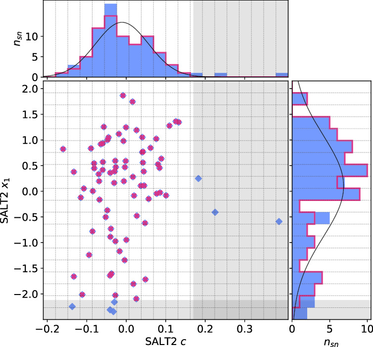
Figure 1. SALT2 c and x1 cuts to better capture a Gaussian “core” for training. The shaded regions correspond to 2σ clippings along the longer tail of each respective c and x1 distribution; blue points correspond to σ-clipped SNe.
Download figure:
Standard image High-resolution imageRelative to G. Aldering et al. (2020), and similar in spirit to K. Boone et al. (2021b), we remove spectra having poor extractions caused by SNR < 3; adjusting this threshold higher up to 10 did not affect our results. This step removes seven spectra, leaving 1148 to train the model.
3. Model
Global template parameters and per-SN parameters are differentiated by upper-case and lower-case characters, respectively. This model discretizes phase and wavelength space, using np = 16 phase nodes ranging from −16 ≤ tp,i ≤ 44 in 4 day intervals; as mentioned in Section 2, nλ = 10 with bins of constant R. Each phase-dependent template is an np × nλ matrix of parameter nodes, while each phase-independent template is a length-nλ vector.
The model prediction of the time-dependent spectral energy distribution evolution of an individual SN Ia is based on a temporal interpolation over a set of wavelength-dependent light curves at fixed phases Fλ,eff that are specific to that SN. The interpolation is controlled by a kernel K, which operates on Fλ,eff as shown in Equation (2). This equation is the same used to predict the mean in a Gaussian process, so we refer to this interpolation scheme as the GPMP:23

These GPMP kernel matrices K specifically are calculated with a stationary p = 2 Matérn covariance function C5/2 to ensure the interpolated curves are twice differentiable:

Fλ,eff is the light curve at wavelength λ on a grid of phase nodes; all nλ = 10 light curves form the flux node matrix Feff. tp,i ∈ tp is a vector indexing the model's np phase nodes and the per-SN parameter t0 aligns said SN Ia's observations with the model's phase grid. Intuitively, the first kernel matrix K in Equation (2) maps each observation to our phase node space after said observation phase ti is translated by t0, while the second accounts for Fλ,eff flux node covariance at grid phases tp,i and tp,j. GPMPs provide a natural framework to translate observed phase ti by the per-SN t0 parameter to the model grid's phase zero-point.
Note that t0 is not the fit date of maximum brightness—instead, t − t0 aligns the observation phase with the model's phase grid tp. As we train the model using rest-frame transformed spectrophotometry, each t0 is fit in its SN Ia's reference z = 0.05 frame. The kernel length scale hyperparameter ρ is fixed to match the phase node interval resolution of 4 days, although the model is insensitive to any reasonable choice in ρ (for example, ρ ≈ 1 week). Furthermore, by fixing ρ = 4, the matrix K is calculated and inverted only once during sampling. The uncertainty hyperparameter σ2 is fixed to unity since it is divided out in Equation (2).
The Feff of each SN is decomposed via element-wise multiplication (also called the Hadamard operation ∘) from a fiducial flux template matrix F0 and a warping matrix Ω:

F0 encodes the training sample's mean flux evolution via a set of fiducial light curves, while Ω encodes deviations from these fiducial light curves for a given SN Ia. Specifically, each column Ωλ of matrix Ω, for a given λ node, is defined as:

Mλ,1 is the λ-node column of the phase-dependent chromatic flux variation template matrix M1. M1 therefore encodes training sample light-curve variation. Lλ,1 and Lλ,2 are the λ-node elements of the two phase-independent chromatic flux variation template vectors L1 and L2, respectively (these appear as scalars in Equation (5) because of their phase independence). Each explicit per-SN parameter is contained within the warping template: the achromatic offset parameter χ0, the phase-dependent chromatic flux variation parameter s1, and the two phase-independent chromatic flux variation parameters c1 and c2. Both differences in intrinsic brightness and peculiar velocity effects are accounted for by the χ0 parameters.
Figure 2 illustrates this model's architecture, specifically displaying the transformed phase-independent template basis  and
and  vectors later discussed in Section 3.3. Figure 3 is a directed acyclic graph of our model. Its conditional probability structure only connects observations to the model flux—deterministic connections (transformations and definitions) are presented with dashed arrows. Global template parameters are located in the top blue box and per-SN parameters in the bottom red box.

Figure 2. A schematic of our model's flux nodes. Each SN Ia has an effective flux node matrix Feff that is an element-wise product of the sample's fiducial flux template F0 and a warping matrix Ω. This warping matrix includes the phase-dependent chromatic flux variation template M1, two phase-independent chromatic flux variation templates  and
and  (which make up the 2D phase-independent chromatic variation model), and per-SN parameters χ0 (achromatic offset), s1 (phase-dependent chromatic flux variation contribution), and c1 and c2 (phase-independent chromatic flux template contributions). Presented here are the
  and
and  basis representation of the phase-independent templates (see Section 3.3 for more information). Per-band nodes are presented in this plot having the same figure color.
Download figure:
Standard image High-resolution image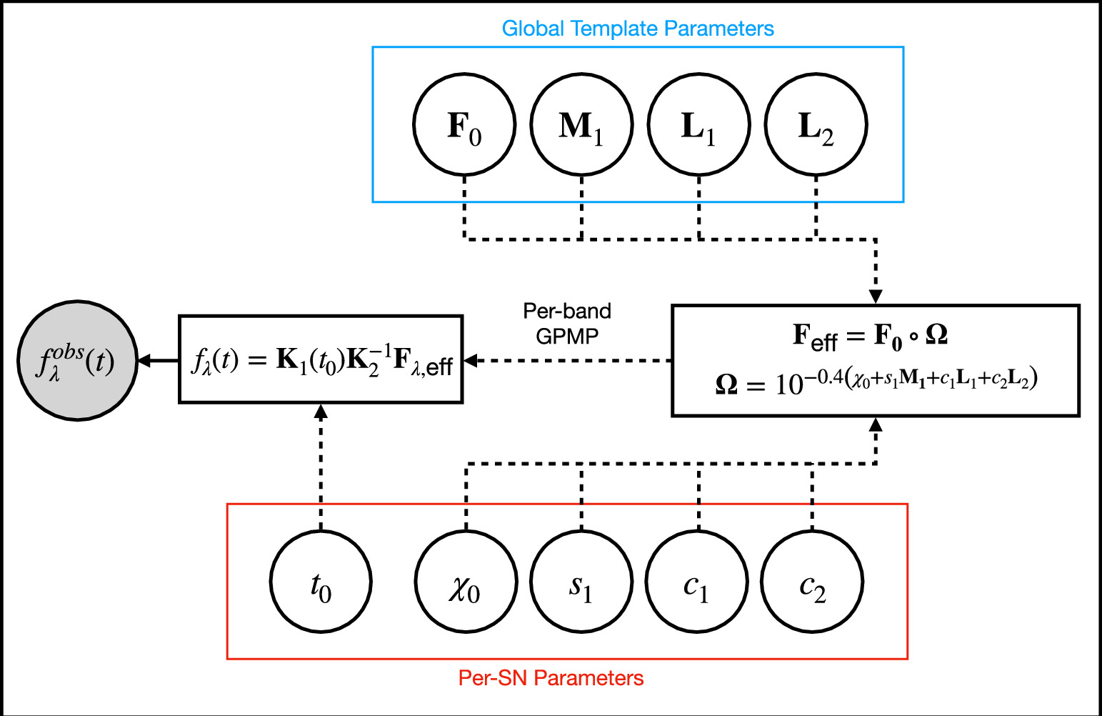
Figure 3. A directed acyclic graph representation of our model. Per-SN model parameters are located in the bottom red box; global template parameters are in the top blue box. The dashed arrows are deterministic relations (transformations and definitions). The only explicit conditional probability in the model's architecture relates observations  to modeled flux fλ(t). We use GPMP interpolation per band in mapping effective template nodes Feff nodes to a predicted flux fλ(t).
Download figure:
Standard image High-resolution image3.1. Template Constraints and Per-supernova Parameter Models
The third λ band, tp,i = 0 phase node of F0 is fixed to 1—it is referred to here as fixed band 3 and corresponds to the wavelength node at 4084 Å, the top-hat filter band closest to a standard B-band. This constraint prevents any scaling degeneracy between F0 and the model's χ0 parameter while also setting the specific phase node that the t0 parameter aligns observations to. Physical consideration further requires all F0 flux node parameters be bound to greater than or equal 0, so we enforce nonnegative values for all flux values.
All chromatic flux variation templates L1, L2, and M1 have scaling degeneracies with their respective per-SN parameters c1, c2, and s1. For example, the transformations s1 → s1/α and M1 → αM1 leave the model unchanged; identical degeneracies exist for c1–L1 and c2–L2. Each scaling degeneracy is removed by requiring these three templates be normalized. This is a straightforward procedure for L1 and L2, where each is instantiated in Stan as unit vectors, but a more involved process is used to normalize the template matrix M1. We first define a unit vector of length np × nλ that is then transformed into M1 by “chopping” said unit vector into nλ column vectors (each of length np) that form the column space of a now normalized M1.24 No further constraints or bounds are placed on the template parameters.
Zero-mean constraints are placed on the per-SN parameter sets c1, c2, and s1. A reference SN Ia could be selected to serve as the c1, c2, and s1 zero-points, but we opt instead to require these per-SN parameter sets to always have a mean of 0. These constraints are enforced structurally by instantiating these parameter sets as centered vectors (Appendix A).
3.2. Fitting the Model
As described in, e.g., C. Saunders et al. (2018) and D. Rubin et al. (2022), the SNfactory data are extracted from the 15 × 15 spaxels of the SNIFS (G. Aldering et al. 2002; B. Lantz et al. 2004) that are projected as spectra onto 2000 × 4000 CCD detectors. In this extraction process the Poisson noise and the readout noise for each pixel are included with appropriate weights. The host galaxy is subtracted from this data cube using a reference data cube taken more than 1 yr later, as described in S. Bongard et al. (2011). Gray dimming by clouds is corrected as described in R. Pereira et al. (2013). The remaining SN-only light is fit with a point-spread function (PSF) model, as described in C. Buton et al. (2013) and D. Rubin et al. (2022), again propagating the Poisson and detector noise uncertainties. Due to small unmodeled PSF shape variations, there is additional uncertainty, which is empirically determined to be approximately 3% (P. F. Léget et al. 2020). The final calculated uncertainties are dominated either by this PSF shape noise or the Poisson plus detector noise.
Initial trial runs confirmed that the nominal uncertainties were underestimated, not having included galaxy-subtraction errors, and that the overall distribution had broader tails than a normal distribution. We thus added a further uncertainty equal to 2% of each SN Ia's maximum observed flux and treat measurement uncertainties as having a Cauchy distribution, which led to stable convergence of the fit. The credibility of this ansatz was checked though inspection of the pull distribution of photometric residuals around the final best fit. This approach has previously been used to represent model uncertainty in B. M. Rose et al. (2021).
The first source of error preferentially increases the high-flux observational errors, while the second largely affects low-flux observations, particularly those 20 or more days after peak brightness. All added uncertainties are diagonal: no covariance is injected into our data before training.
The nominal SNfactory measurement and uncertainty are used as the Cauchy distribution location and scale. For each flux observation  with its corresponding measurement uncertainty
  , our likelihood function takes the form:

No correlations are added between measurement errors.
The model is implemented and trained using the statistics programming language Stan (B. Carpenter et al. 2017). Built into Stan is a No U-Turns (NUTS) Hamiltonian Monte Carlo (HMC) sampler well suited for sampling our model's high-dimensional posterior. No explicit priors are placed on the templates or per-SN parameter sets, instead leaving them with default implicit flat priors along any aforementioned bounds (Section 3.1).
Stan is informed with initial conditions estimated by first running simpler versions of the model. We do this only to improve sampling efficiency—it is not necessary for our model's convergence. This process is done iteratively, starting with the simplest model that only obtains the t0, F0, and χ0 parameters (a mean light-curve model). The results of this simplest model then become the initial conditions for a more complex model that includes the L1 and c1 parameters. Other components (specifically, L2 and c2, and then M1 and s1) are then added and trained using the prior model iteration's fit as initial conditions until all the described model's components are incorporated. Note that we use SALT2's  as initial conditions for the t0 parameters when training the simplest of these models.
With Stan's default NUTS we pull 4000 samples for each of 16 types of instantiated samplers: 2000 warm-up followed by 2000 samples iterations per chain. Stan is run on the University of Pittsburgh's Computational Resource Center.25
The convergence metrics “split- ” and “effective sample size” were calculated after postprocessing using techniques provided in A. Vehtari et al. (2021). After training and postprocessing, each SN Ia is refit with the template parameters fixed (F0, M1, L1, and L2) to determine the final values for the per-SN Ia χ0, s1, c1, and c2, permitting a direct comparison of these per-SN parameters against other empirical SN Ia models.
There is no selected standard ΔMB = 0 SN Ia identified in the training sample, leaving a nontrivial linear degeneracy between the achromatic offset parameter χ0 and phase-independent parameters c1 and c2. For physical reasons, c1 and c2 should not correlate with the intrinsic magnitude, which ideally should only be captured by χ0.
Linear transformations from P. F. Léget et al. (2020) are used to remove correlations between both the c1 and χ0 parameters, and the c2 and χ0 parameters, as summarized in Appendix B. Implementing this directly in the Stan model leaves the results unchanged but does reduce the sampling efficiency, so this step is performed after sampling.
3.3. Interpreting the Phase-independent Templates
Each sampler from Stan explores a plane spanned by the template vectors L1 and L2.26
Even after decorrelating χ0 from c1 and c2, the output basis {L1, L2} is not unique, a consequence of this model's physics-agnostic architecture. This is because for any nonsingular linear transformation the output basis vectors (i.e., aL1 + bL2 and cL1 + dL2 for  and ab − cd ≠ 0) necessarily span the aforementioned plane. To quantify this plane's convergence (as opposed to only its basis vectors), for each posterior sample we calculate a bivector
  that, by definition, spans the plane of interest. Importantly, the bivector representation
  is no longer ambiguous.
A bivector is a geometric object representing an oriented plane element constructed from the wedge product (see Figure 4 for an illustration). Intuitively, a bivector corresponds to a plane like a vector corresponds to a line, and the wedge product is the dual to a cross product in 3D. Unlike the cross product, the wedge product generalizes to any finite-dimensional vector space greater than 2, meaning bivectors are well-defined in this model's 10D wavelength node space. Now any SN Ia'a phase-independent chromatic flux variation curve c = c1L1 + c2L2 can be interpreted as residing in the plane spanned by  , regardless of the selected L1, L2 basis.
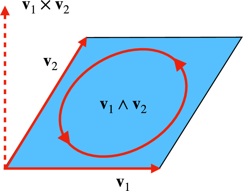
Figure 4. This is an illustration of a bivector (the blue parallelogram) v1 ∧ v2 constructed by the vectors v1 and v2 (the red vectors) in 3D. A 3D space allows for the corresponding cross product to be included for reference (the red dashed vector). Bivectors, like vectors, are oriented objects, with the bivector v1 ∧ v2 having a counterclockwise orientation determined by component vector ordering (here represented with an oriented red loop). Reversing the product order reverses a bivector's “circulation” or orientation: v2 ∧ v1 = −v1 ∧ v2. Note that the cross product does not generalize to all finite-dimensional vector spaces, while the wedge product ∧ does.
Download figure:
Standard image High-resolution imageEach component of the bivector  is calculated as follows:

where  is the ith wavelength component of template L1 and
  is the ith wavelength component of template L2. Importantly, this representation is independent of the L1, L2 choice. Note that
  is normalized so as to represent a unit plane element. With these transformed parameters
  , the model can unambiguously be tested for convergence and the best-fit templates be determined.
3.4. Bases for the Phase-independent Chromatic Variation Model
We now seek a pair of vectors, L1 and L2, that span  and readily provide insight into the physical origin of the model's 2D phase-independent chromatic flux model. Two such bases are considered.
3.4.1. Maximum Variance Ratio Basis
The first basis, called the maximum variance ratio (MVR)27 basis, is derived directly from the corresponding c1–c2 distribution.
New and uncorrelated parameter sets  and
and  with their relative variances maximized are found via a linear transformation. The result is a basis for
  where
where  accounts for the most chromatic flux diversity by a single template in
  , while
  captures any remaining variation. This basis amounts to the assumption that two independent physical effects affect chromatic flux variation (e.g., the amount of dust or intrinsic SN Ia diversity) while designating as much of the variance as possible to one source (e.g., dust). This assumption provides some useful insights even if it does not totally satisfy our physical expectations, as it does not consider additional possible effects (e.g., the kind of dust), nor that SNe and their progenitor environments likely correlate with said effects. This basis's solution is found by numeric minimization; it is not orthogonal.
The MVR basis is determined as follows. A basis centered at the origin can be described by the angle between the unit vectors and their orientation. Starting with an orthogonalized output basis from Stan ![${\boldsymbol{L}}=[{{\boldsymbol{L}}}_{1}^{\,\rm{orth}\,},{{\boldsymbol{L}}}_{2}^{\,\rm{orth}\,}]$](https://content.cld.iop.org/journals/0004-637X/982/2/110/revision1/apjad9f32ieqn28.gif) for
for  and a per-SN coefficient matrix c (here arranged as an nsn × 2 matrix), adding an extra angle θ between the basis is achieved with the transformation:

In this  basis, the per-SN coefficients
  have an orientation given by VT from the singular value decomposition (SVD) of
  . Taking VTM and normalizing its rows to be unit vectors gives the properly oriented basis given θ. Note that these primed components here are unrelated to those introduced below.
For this basis, the ellipticity of its corresponding c distribution is again found using SVD, given by  . An optimizer is used to determine the θ that maximizes the ellipticity.
3.4.2. Cardelli–Clayton–Mathis-derived Basis
We also desire a basis that readily separates rapidly changing chromatic flux variation (i.e., that akin to SN absorption/emission features) from continuum-like chromatic flux variation (i.e., dust-like behavior). This continuum-like variation is assumed to be dust-like, given dust extinction's ubiquitous contribution to SN Ia color/chromatic flux variation. The two phase-independent plots found in Figure 2 provide an example of what we want from this basis—specifically, one template being more smooth with respect to wavelength than the other.
For the second basis, the vector  simultaneously resides within the planes spanned by both
  and the Cardelli–Clayton–Mathis (CCM89) dust model (J. A. Cardelli et al. 1989), defining the first basis component. This intersection ensures it captures smooth, CCM89-like chromatic variability. The other basis vector
  is chosen to be perpendicular to
  , while still residing in the
  plane; this basis is orthogonal by construction. Note that
  will not necessarily be perpendicular to the plane spanned by CCM89, but is still guaranteed to provide the least continuum-like variability with respect to (w.r.t.) wavelength (and therefore, the most spectral-feature-like behavior) allowed by
  . This basis provides a useful representation not because it recovers a mathematically valid dust extinction curve, but instead because it clearly separates rapidly changing chromatic flux variation from SN continuum-like variability. It is important to remember that intrinsic variability could still affect the direction of the first basis vector
  , which means this basis does not guarantee a physical decomposition into exclusive dust and intrinsic components. As such, any dust-like properties inferred from L1 in isolation are physically ambiguous.
The CCM89-derived basis is calculated as follows. Since CCM89 has two basis curves a(λ) and b(λ) (one for each parameter AV and AV/RV, respectively), one can construct a CCM89 unit bivector  from discretized curves a(λ) → a and b(λ) → b using an appropriately modified version of Equation (7):
  and
and  . The two planes spanned by
  and
and  then intersect within the nλ-dimensional wavelength vector space along a line. It is the vector which spans this intersecting line that defines the new
  template:

We are free to choose a new L2 as long as it resides within the subspace represented by  . To minimize this L2 template's dust-like properties,
  is defined as a θ = π/2 radian rotation of
  within the plane spanned by
  via a rotation operator
  :
:

This rotation maximizes the component of  that is perpendicular to the plane spanned by
  . The new
  also transforms the c1 and c2 parameters sets, here labeled
  and
and  .
.
Figure 5 provides a 3D view of the geometric intuition involved in finding the CCM89-derived basis. All calculations discussed here are implemented using geometric algebra, which provides a novel approach to study oriented subspaces. Geometric algebraic implementations for calculating intersections, projections, and rotation operations are summarized in Appendix C. Although we exploit geometric algebra's elegance and interpretability to perform all said operations, each operation could be done using more classical linear algebraic techniques if desired.
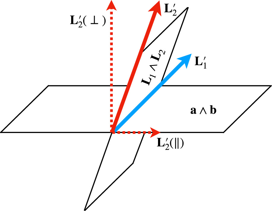
Figure 5. A 3D representation the CCM89 basis's geometric intuition. The blue solid vector is the transformed  template spanning the intersection of two planes, one spanned by the model bivector
  and the other spanned by the CCM89 bivector
  . The red solid vector is a π/2 rotation in the plane spanned by
  that defines the transformed
  template. The decomposition
  with respect to the CCM89 plane spanned by
  is given with the red dashed arrows.
Download figure:
Standard image High-resolution image3.5. Handling Similar Solutions
In training, the samplers converge to one of three sets of very similar solutions, as is apparent in the per-chain values of L1 shown in Figure 17. We find that simultaneously obtaining global template and per-SN parameters leaves the resulting samplers sensitive to the three least representative SNe Ia in the training sample (based on residuals). These groups are associated with slightly different solutions for these three SNe Ia, as seen by eye and quantitatively through their χ0 solutions. Consider the following analogy: consider the inertia tensor of a space station as being the model's global templates and the coordinates of its crew members corresponding to the per-SN parameters. The moment of inertia changes only slightly if crew members move to another location on the station (assuming the space station is much more massive than the crew's total weight). Similarly, it is this “change in position” of per-SN solutions that is causing a very subtle change in template parameters, preventing complete convergence. Obviously this is not a fair comparison, but the resulting effects are very similar, hence this comparison.
The worst performing SN Ia PTF11mkx consistently sees a 1σ difference between χ0 values between different chain groups—considering that this χ0 parameter fit uncertainty is only ≈1%, this tail wagging is very subtle. Indeed, when refitting per-SN parameters with one of the group solutions as a fixed global template (Section 4.4), all chains converge to the same solutions for the three SNe Ia. Similarly, if two different group solutions are separately held constant and refit individually, the two resulting per-SN parameter sets are indistinguishable. Because each group's solutions are consistently very similar, we opt to use the weighted average of all solutions for the best-fit template. This decision to use an average of all groups, as opposed to using a specific solution, has no impact on the remaining analysis.
Note that refitting with a fixed t0 parameter does not prevent this subtle grouping, nor does cutting these three SNe Ia from the training set. If these three aforementioned troublesome SNe Ia are removed, the next few SNe Ia that are the least representative of this newly trimmed sample start “wagging.” This instability may be a feature of our model. In particular, the flat priors we use for the c1 and c2 distributions may bias the results for the least representative SNe Ia of a given training sample. Considering that global template parameters again were effectively unchanged with their removal, we retain those three SNe Ia for the remainder of the analysis.
4. Best-fit Model Results
Our model, as implemented with Stan, consists of global template parameters and per-SN parameters. We define the best-fit solution to be the mode of a 365D template parameter space,28 with each per-SN parameter marginalized before estimating from HMC sampling the posterior's maximum. This mode is estimated using a mean shift clustering algorithm implemented in the scikit-learn package using the default flat kernel (F. Pedregosa et al. 2011). To estimate a consistent best-fit solution, bivector components L = L1 ∧ L2 (Equation 7) are used instead of the L1 and L2 components directly. This process is analogous to maximum a posteriori estimation of the HMC-sampled posterior, but allows first for the aforementioned postprocessing. The marginal posterior dispersion for each parameter is presented as 68th percentile error bars. The residuals of the best-fit model, alongside binned averages, are presented in Figure 6.
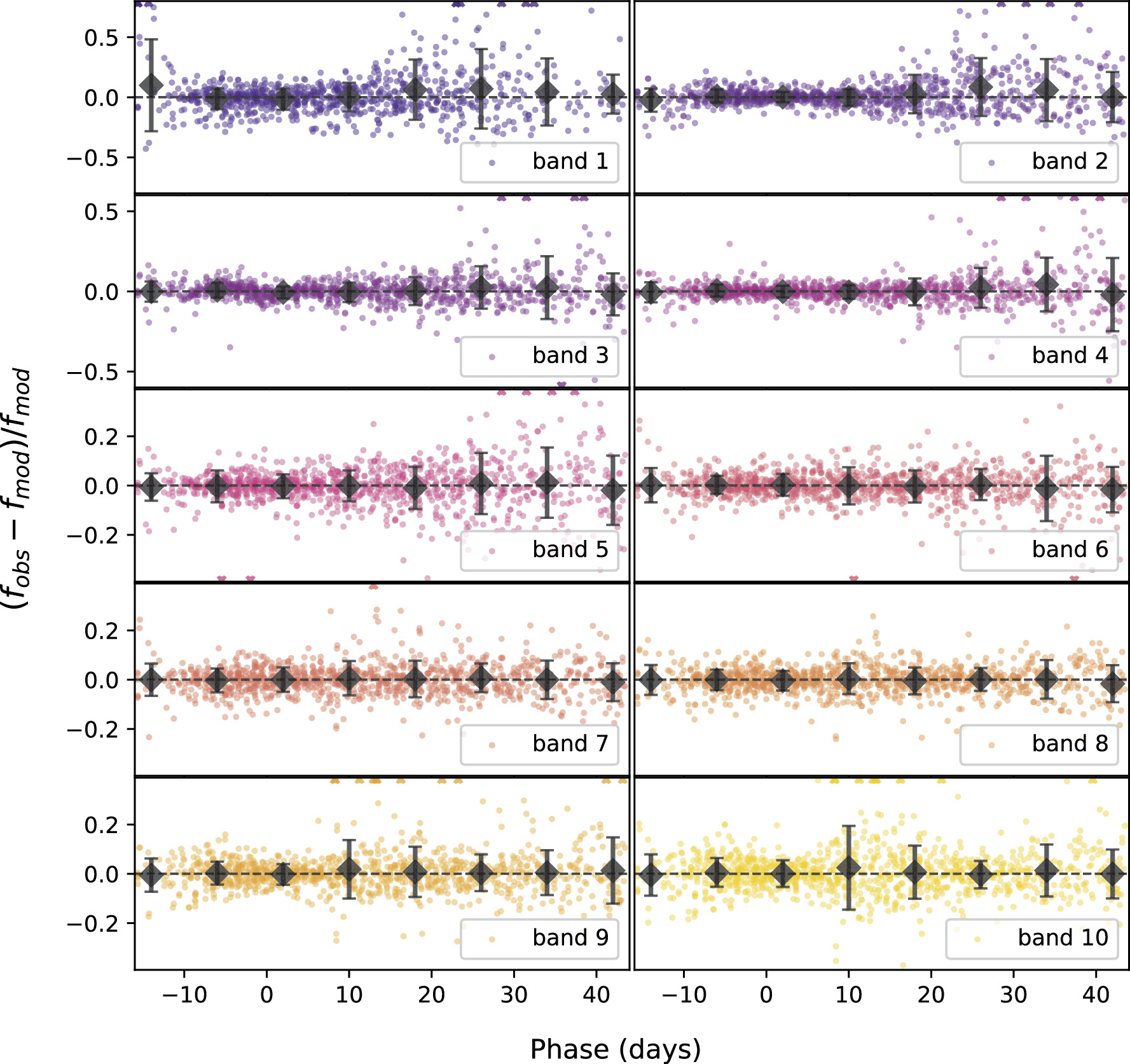
Figure 6. Best-fit model residuals with respect to observations presented for each of our 10 bands. Eight day binned averages for each band are presented as black diamonds, with error bars being binned standard deviations. The carets at the top and bottom edges represent points that lie outside the range of the plots.
Download figure:
Standard image High-resolution imageTwo of the 16 HMC samplers were rejected after fitting because (1) their resulting mean t0 parameter values were systematically inconsistent by 4 to 5 days with SALT2 date of maximum, 2) the corresponding light-curve shapes were nonphysical, and (3) these two samplers have notably inconsistent  values relative to the 14 retained samplers. The 14 remaining samplers converge to three very similar group solutions of which the weighted average is taken; see Section 3.5 for more details.
Table 1 provides the median values and 68th percentile upper and lower values for the per-SN light-curve model parameters.
4.1. Phase-independent Chromatic Flux Variation Templates
Ostensibly, if  were to only capture CCM89 dust-like behavior, then the planes spanned by
  and
and  would be effectively parallel and any intersection poorly constrained. This turns out to not be the case, with the best-fit solution recovering a planar separation angle of about 80∘.
4.1.1. Maximum Variance Ratio Basis
Figure 7 presents the MVR basis as described in Section 3.4. Qualitatively,  appears nominally more dust-like than its counterpart
  . Figure 7 includes the best-fit CCM89 curve
  for reference, showcasing that its most extreme divergence from CCM89 is blueward of 5000 Å.
  , on the other hand, captures variation that is not readily describable as dust-like: normal dust extinction should be absorptive across the optical wavelength range whereas the sign flip in
  produces simultaneous brightening/dimming on either side of 4000 Å. Although the degree of variation increases as wavelength decreases, there is a distinct flip in behavior around 4000 Å. Such behavior is inconsistent with dust extinction.
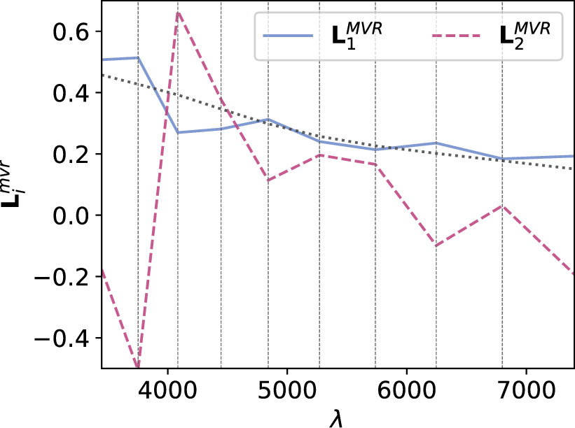
Figure 7. The blue solid line corresponds to the first MVR component  , which appears nominally more consistent with dust-like variation than its counterpart
  , given as the magenta dashed.
  has a best-fit
  given as the gray dotted line, with most of its divergence from a CCM89 curve occurring blueward of 5000 Å.
  captures variation not readily describable as dust-like.
Download figure:
Standard image High-resolution imageThe conditions for the target parameter set distributions are to assign maximum variance to one component while keeping the second component uncorrelated. These conditions yield a basis consistent with the expectation that dust-like variation is the primary contributor to SN Ia phase-independent chromatic flux variation while intrinsic SN Ia diversity uncorrelated with dust accounts for additional variability.
4.1.2. Cardelli–Clayton–Mathis-derived Basis
The template  is presented in the top plot of Figure 8. As summarized in Section 3.4, the intersection of the plane spanned by
  with the plane spanned by
  defines the first phase-independent chromatic flux template
  . This
  template, as expected, captures continuum-like variation akin to dust extinction.
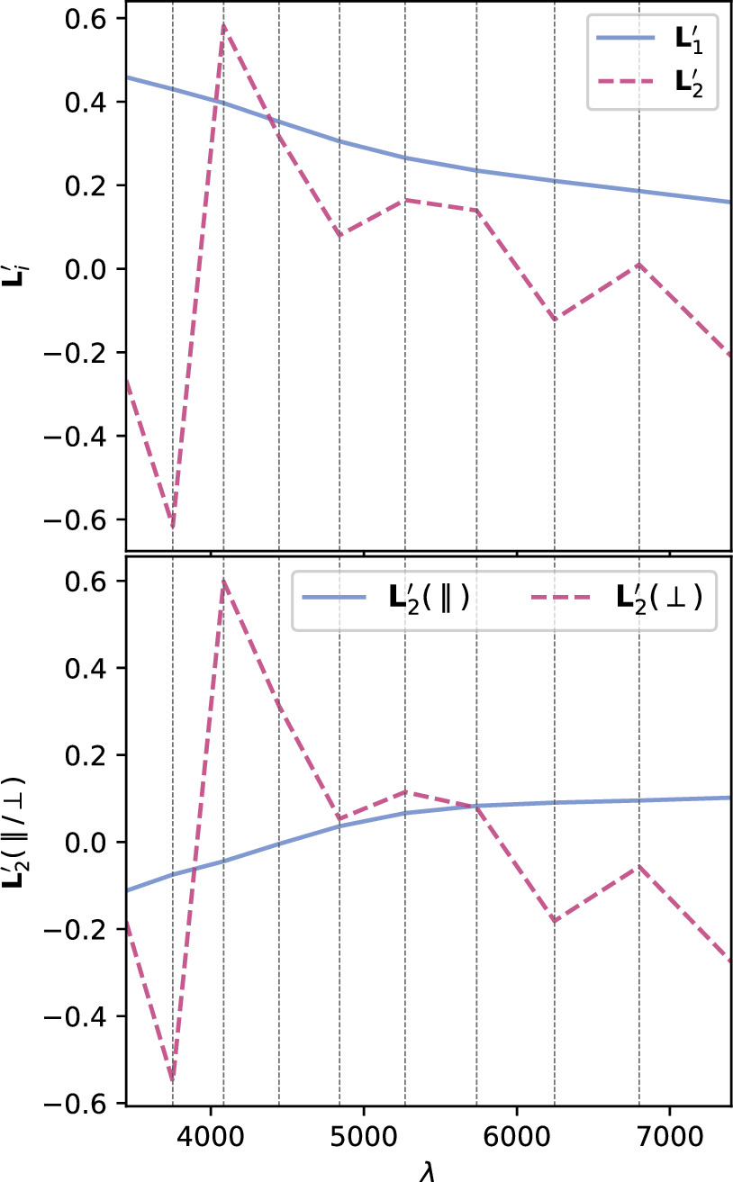
Figure 8. The top plot presents phase-independent chromatic flux variation templates  and
and  .
.  has a recovered total-to-selective extinction of
  . The bottom plot presents a decomposition of
  into its parallel and perpendicular components with respect to the CCM89 plane.
  clearly captures some dust-like variability, despite being dominated by intrinsic modes. Although the low-resolution wavelength binning prevents quantification of spectral features, the most impressive
  variability appears in the Ca ii H and K regime.
Download figure:
Standard image High-resolution imageFrom  we find an intersection total-to-selective extinction ratio of
  . As mentioned in 3.4, this RV is not immediately physically interpretable without an AV model.
Also presented in the top plot of Figure 8 is template  . Unlike
  ,
,  captures the more rapidly changing flux variability allowable by
  . Specifically, L2 is capturing wavelength variation at scales smaller than that expected by continuum dust variability, at least within the optical regime. Indeed, its features nominally align with spectral features. Also note the similarity between
  and
and  despite their vastly different constructions.
 is not perpendicular to the CCM89 plane because the plane spanned by
  is itself not perpendicular. As such,
  also captures a dust-like component alongside its dominating spectral-like component. The bottom panel presents this template's decomposition into parallel and perpendicular components defined with respect to CCM89's plane for reference.
4.1.3. Intrinsic Variation
Both of the best-fit template representations  and
and  capture pronounced phase-independent chromatic flux variation blueward of 4500 Å that is inconsistent with dust (see Figure 9). Indeed, no extrinsic phenomena readily describe this behavior. Variation blueward of 4500 Å includes the prominent Ca ii H and K feature and its Si iii counterpart, Si ii λ4130, C ii λ4267, Fe ii λ4404, and Mg ii λ4481. With our choice of splitting the spectral range into nλ = 10 synthetic filters, the model cannot completely distinguish between said features, although at least one node for both
  and
and  and their corresponding variation seemingly align with the wavelength bin where Ca ii H and K is the dominant contributor to a strong spectral feature; Si ii and Fe ii features also contribute to this variation. Hints of chromatic flux variability ostensibly aligns with the SNe Ia signature Si ii λ6347 feature and O i λ7774, which are visible in Figure 8, but in practice do not affect any resulting model flux predictions (again, see Figure 9).
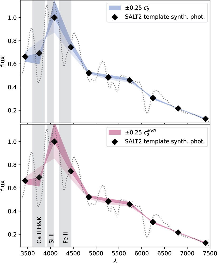
Figure 9. This figure demonstrates a ± 0.2 mag c2 variation (blue for the CCM89 basis  , maroon for
  ) of
) of  overlaid on SALT2's mean template t = 0 phase spectrum (dashed black line). The spectrum is binned via synthetic photometry with top-hat filters, presented as black diamonds. Flux units are normalized by synthetic photometry wavelength 4048 Å value to unity and example spectral features blueward of 4500 Å are presented for reference.
Download figure:
Standard image High-resolution imageWe use the same data set used by C. Saunders et al. (2018) for their SNEMO analysis. Comparing both  and
and  to SNEMO2 and SNEMO7 eigenvectors (with two and seven components, respectively) yields indecisive insight, though. Figure 6 from C. Saunders et al. (2018) shows SNEMO eigenvectors describing similar
  or
or  behavior at maximum, but all of these eigenvectors are clearly phase dependent—no eigenvector's evolution seems approximately phase independent. Figures 9 through 12 from C. Saunders et al. (2018) present some unexplained variation for SNEMO2 blueward of 4500 Å that is nominally phase independent up to 6 days postmaximum; this all but disappears with SNEMO7. That SNEMO2, itself similar to SALT2, sees unexplained phase-independent variability around maximum that aligns with the
  and
and  features seems indicative of our model's performance, but such a claim taken alone is likely an excessive interpretation.
SNfactory data are also used by K. Boone et al. (2021b) with their Twins Embedding nonlinear model. More interesting insight is gained in comparing their findings with our template representations  and
and  , since Twins Embedding is currently a phase-independent, maximum-phase model. Blueward of 4500 Å, spectral variation recovered by Twins Embedding loosely aligns with the both
  and
and  templates (see Figures 4, 6, and 10 from K. Boone et al. 2021a for reference). Recovering this consistent variation in our phase-independent template, albeit at lower wavelength bin resolution, lends credibility that
  as a whole is capturing intrinsic variation.
Past analyses by D. Branch et al. (1993) and A. G. Riess et al. (1998b) find Ca ii H and K features are relatively stable in the week before and weeks after peak B-band brightness, with this effective phase independence being sufficiently stable to exploit for the latter's “snapshot” methodology from which they constrain luminosity distances. Both  basis representations do capture intrinsic, phase-independent variation around Ca ii H and K, but this alone is not profound evidence of fundamental Ca ii H and K time independence in the SN Ia population. SN Ia Ca ii H and K features, as with all spectral features, demonstrably evolve with time. In its current form, this model cannot distinguish between phase-averaged spectral variation or truly phase-independent intrinsic variation. Indeed, a goal of this project is to demonstrate that intrinsic chromatic flux variation can “leak” into phase-independent components, something that is occurring in these results.
4.2. Fiducial Template
Figure 10 presents GPMP interpolations of each band's best-fit Fλ,0 nodes as solid curves. The fixed band 3 template is the third solid curve presented in the top plot of Figure 10. The ubiquitous NIR bump is recovered for redder bands (bottom plot of Figure 10), with this second maximum occurring ≈25 days after our fixed-band peak brightness as expected (S. W. Jha et al. 2019). Apart from the reddest template curve centered at 7401 Å, the peak brightness phase per band occurs earlier for bluer bands and later for redder bands, again consistent with established trends (S. W. Jha et al. 2019). As would be expected by its I-band overlap, the reddest template curve exhibits somewhat more complex behavior than the other curves, such as the inflection point between its two local maxima (bottom plot, Figure 10).
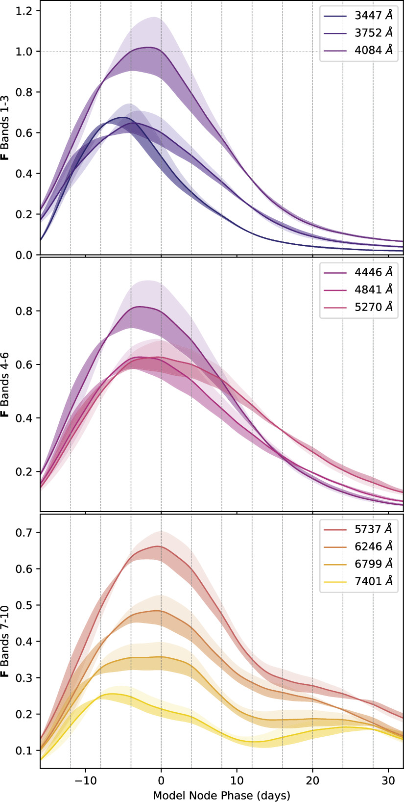
Figure 10. A visualization of ±0.09 mag variation in s1 on the model's fiducial flux template F0, as warped by the phase-dependent chromatic flux template M1. Positive s1 contribution is given by light shaded regions, while negative s1 contribution is given by the dark shaded regions. Solid lines are the GPMP-interpolated light curve for that band's fiducial template nodes, which is deterministic (not stochastic) in our model. The top two plots illustrate recovered stretch-like behavior by the template M1, with broadening to narrowing of the effective light curve as s1 increases in value. The bottom plot captures stretch-like behavior further convolved with NIR bump variational modes (bump location and size). Note that these figures are not portraying model uncertainty, only model response to s1 parameter variation.
Download figure:
Standard image High-resolution imageNote that each fiducial template light curve's peak brightness phase does not align with our tp,i = 0 flux node, meaning t0 should not be interpreted as the fixed band 3's peak brightness phase. This is ultimately inconsequential, requiring only that each light curve's peak brightness phase be calculated deterministically after fitting, and has no effect on this analysis or its conclusions.
4.3. Phase-dependent Chromatic Flux Variation Template
As shown in Figure 10, the best-fit phase-dependent variation template M1 exhibits stretch-like behavior across all bands. The shaded regions in these plots show phase-dependent light-curve variation from −0.09 < s1 < 0.09 mag, which approximately captures the dispersion of the fit s1 parameter set (the set's standard deviation is 0.09 mag). The lighter shaded regions correspond to positive s1 values, while the darker correspond to negative values. As s1 increases (decreases), the Feff node values increases (decreases) with respect to F0's node values, resulting in each GPMP interpolation curve's global maximum decreasing (increasing). This change in Feff node scaling is offset for by a change in χ0, correlating the χ0 and s1 parameter sets (see Section 4.4).
The sign of M1 template's contribution is a function of phase: for each curve there are two phases where the M1 template's contribution reverses in sign. For positive (negative) s1, the result is a narrowing (broadening) of the effective flux curve. The phase and degree of this broadening varies between bands in a manner consistent with D. Kasen & S. E. Woosley (2007), being more extreme for bluer wavelengths. Furthermore, Figure 11 plots our model's Δm3(15) as a function of s1, demonstrating our M1 template indeed recovers stretch-like behavior for this model's B-band analog fixed band 3.
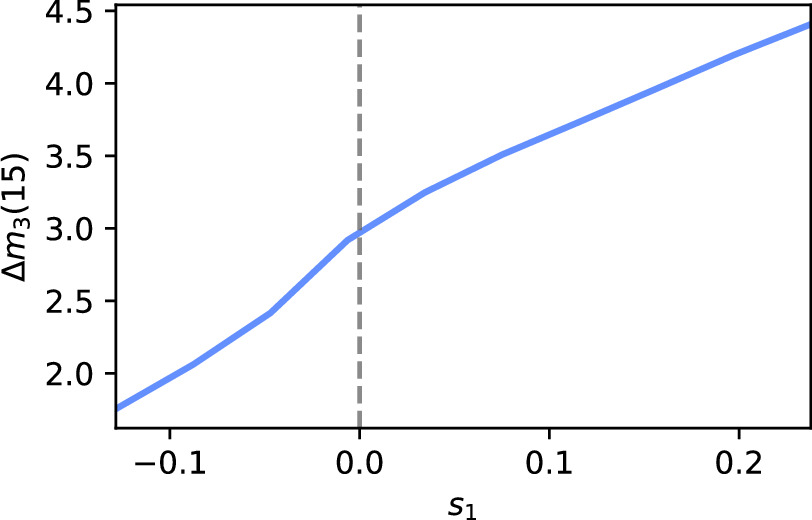
Figure 11. The model's Δm3(15) (the ΔmB(15) analog for the fixed band 3) as a function of s1 calculated for the fixed band 3 along the training sample's obtained s1 value range.
Download figure:
Standard image High-resolution imageFor redder bands, stretch-like behavior is convolved with NIR bump variation (bottom plot of Figure 10). A 3D mesh plot (Figure 12) best illustrates these two modes of NIR variation: bump depth and bump location. As expected, these variation modes also correlate with stretch (C. R. Burns et al. 2011; S. Dhawan et al. 2015), with stretch appearing as the valley-like feature in Figure 12.
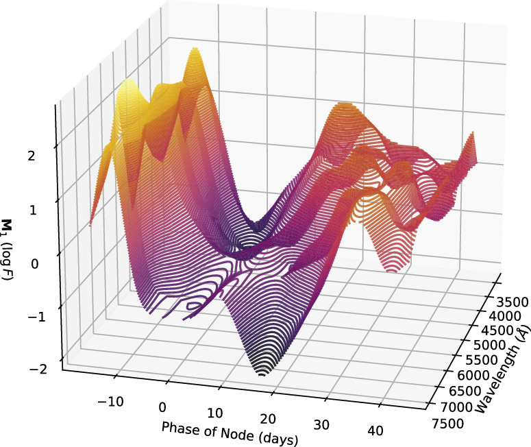
Figure 12. A contoured 3D view of our phase-dependent variation template—this is our model's equivalent to SALT2's M1 stretch template. The valley-like structure corresponds to stretch-like behavior extracted by our M1 template.
Download figure:
Standard image High-resolution imageFor fixed band 3, the phase of maximum brightness relative to our zero-phase node is a function of s1. This movement in maximum brightness location, made clear in Figure 10, ranges from +1 day for our most negative s1 = −0.15 mag SN Ia to −3 days for our most positive s1 = 0.22 mag. Again, this has no effect on our analysis, requiring only an a posteriori calculation at the phase of maximum brightness if desired.
4.4. Per-supernova Results
Each SN Ia is refit with template parameters fixed to the previously discussed best-fit solution. Scatterplots comparing parameter sets include Spearman rank correlation coefficient (SCC) calculations alongside corresponding p-values. For color, only the CCM89-derived basis parameter sets  and
and  are presented. As the MVR and CCM89-derived bases yield parallel
  planes, we choose to present results from the latter since the CCM89-derived basis is more readily interpreted—its first component is, by definition, a mathematically valid CCM89 curve. Note that we do not compare per-SN parameter sets from different basis decompositions.
In Figure 13, per-SN parameter sets for  ,
,  , and s1 are compared with their corresponding χ0 values. The measured SCC value of 0.59 between the training sample's s1 and χ0 parameter sets results from a varying s1 changing the resulting Feff scaling, requiring a compensating change in χ0 to offset (see Section 4.3). By construction, the
  and
and  sets are de-correlated with χ0 (see Section 3.3). Higher rank correlations are recovered for
  versus s1 and
  versus
  compared to
  versus s1, as seen in the scatterplots of Figure 14.
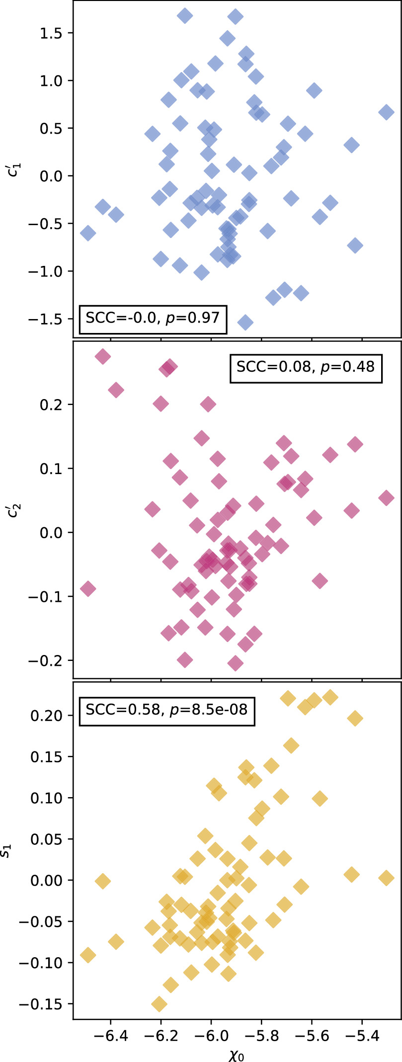
Figure 13. Comparison of fit  (top, blue),
  (middle, magenta), and s1 (bottom, yellow) samples against our χ0 samples. The correlation between χ0 and s1 arises from s1's changing of Feff's scale, which is then compensated for by a change in χ0. There are no correlations between either
  and χ0 or
  and χ0 by construction.
Download figure:
Standard image High-resolution image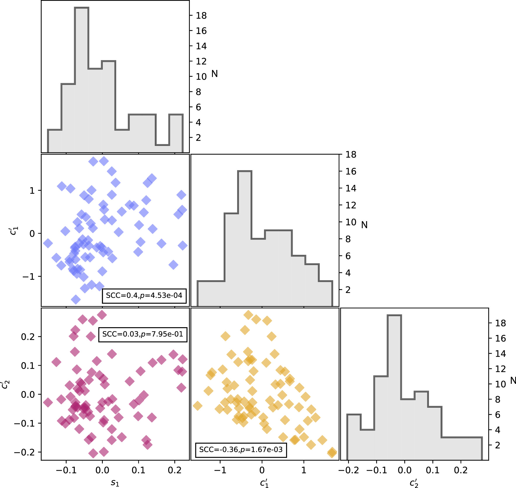
Figure 14. Corner plot for the per-SN parameters s1,  , and
, and  . Magenta points compare s1 and
  , yellow points compare
  and
and  , and blue points compare
  and
and  parameter sets. We measure only marginal rank correlations between both
  vs. s1 and
  vs.
vs.  . N is the number of SNe Ia.
Download figure:
Standard image High-resolution imageWe also quantify the fractional variance of the  and
and  bivariate distributions not explained by CCM89-like behavior. Each SN Ia phase-independent chromatic flux variation vector
  is first normalized. The perpendicular component with respect to the CCM89 plane spanned by
  of each normalized c is then calculated via a projection operation (see Appendix C.2). This resulting distribution has a median value of 0.13 with 68th percentiles [0.05, 0.4] and provides a measure of our sample's fractional variance attributable to captured phase-independent chromatic variability which is not dust-like. Unsurprisingly, dust-like variation, which explains the remaining ≈87% variance, dominates the captured phase-independent variability. Even if this dust-like variation was the exclusive result of actual dust extinction (no “leaking” of intrinsic variability into dust-like behavior), the remaining ≈13% variance, which instead arises from intrinsic variability in the sample, is not negligible.
  , with
  in particular, is capturing a discernible addition of SN Ia variation over past two-component models (i.e., SALT2).
4.4.1. Comparison to SALT2
This new SN Ia model and SALT2 are trained using optical wavelength observations, with neither making assumptions about dust extinction, making SALT2 an obvious comparator. One technical difference is our model's accounting for phase-dependent variability with a multiplicative variation template as opposed to SALT2's flux variation linear component, which is obviously additive in flux space. Nonetheless, s1 and x1 should correlate. This is the case as seen in Figure 15, with a rank correlation of −0.89 between x1 and s1. As presented in Section 4.3, this model's M1 templates obtains stretch-like behavior, just as SALT2's first-order variation template M1(t, λ) does.
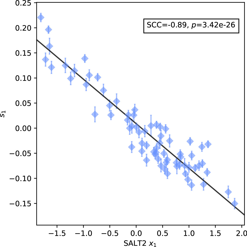
Figure 15. Per-SN comparison of our stretch parameter s1 vs. SALT2's stretch proxy x1. An ordinary least squares linear best fit is provided with a solid black line. Error bars correspond to 68th percentiles.
Download figure:
Standard image High-resolution imageThe phase-independent chromatic flux variation template basis  is selected without consideration of SALT2's CL(λ) phase-independent chromatic variation model. As such, any correlations between
  or
or  and SALT2 c are nontrivial—as seen in the top plot of Figure 16, only SALT2 c and
  are correlated with a rank correlation of 0.78. Considering
  is the maximal CCM89 dust-like vector allowed, that SALT2 c and
  are strongly correlated is because SALT2's CL(λ) template predominately captures dust-like variation. Indeed, the latest SALT3 recovers a CL(λ) curve that is consistent with SALT2 and similarly aligns with CCM89 between 4000 and 7000 Å (W. D. Kenworthy et al. 2021). As seen in Figure 13 of W. D. Kenworthy et al. (2021), both of the SALT2 and SALT3 CL(λ) templates begin to diverge from CCM89 near where
  starts to exhibit most of its variability.
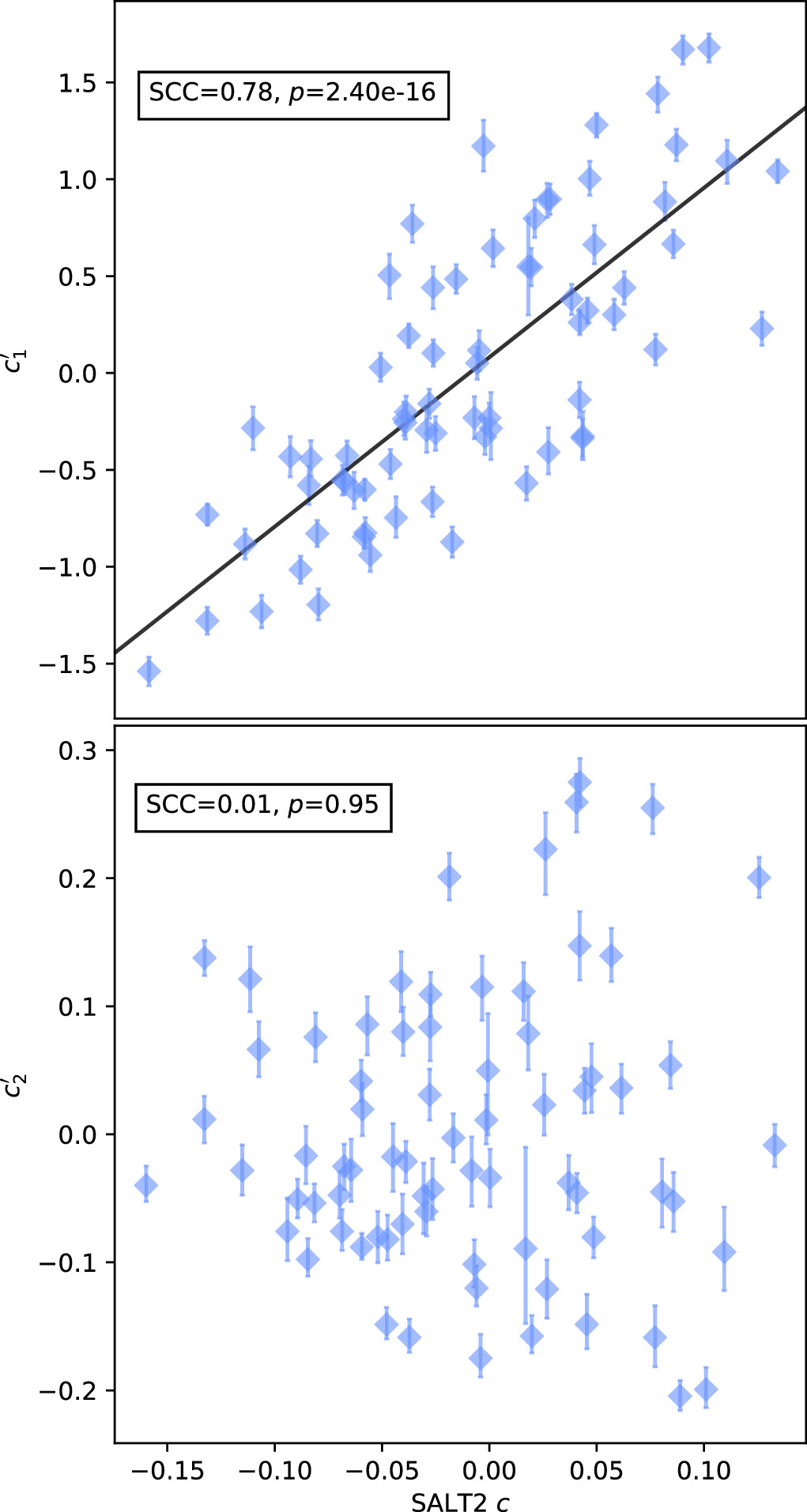
Figure 16. A per-SN comparison of our per-SN chromatic flux variation parameters  (top) and
  (bottom) against SALT2's c parameter. We measure a clear rank anticorrelation between
  and SALT2 c, but measure no correlation between
  and SALT2 c. We interpret this as template
  capturing chromatic flux variation not modeled by SALT2. An ordinary least squares linear best fit between
  and SALT2 c is provided by a solid black line. Error bars correspond to 68th percentiles.
Download figure:
Standard image High-resolution imageThe bottom plot of Figure 16 demonstrates that the  and SALT2 c parameter sets are uncorrelated. As one would hope, the presented model's two-component phase-independent chromatic variation model captures SN Ia variation beyond that of SALT2. For reference, we provide best-fit linear relationships between SALT2 x1 and s1, and between SALT2 c and
  :
:


5. Conclusion
In this article, we introduce a new empirical SN Ia linear model that expands beyond similar analyses by introducing a second phase-independent chromatic flux variation template into its architecture. Our model converges to a solution with three variation components: one phase-dependent chromatic flux variation template M1 and two phase-independent chromatic flux variation templates L1 and L2, which are represented together by the bivector  . The phase-dependent model component recovers stretch and NIR bump variation; it along with the phase-independent templates are consistent with SALT2's two model components.
The model's extended phase-independent architecture captures a nuanced combination of variability. Analysis of the 2D phase-independent chromatic flux variation plane spanned by  is done two bases: one that maximizes variation ratios (MVR) between the c1 and c2 parameter sets, and another that is defined with respect to the CCM89 dust plane. The MVR approach recovers nominally dust-like variation for its dominant component
  , with a fit
  , while
  trace potentially low-resolution intrinsic features. The CCM89 basis yields similar, albeit somewhat more physically interpretable, results. Specifically, this basis naturally decomposes
  into one template capturing continuum-like wavelength variation (
 ) and another capturing rapidly changing chromatic flux variation w.r.t. wavelength (
 ). Component
  is defined as the intersection of our model's phase-independent chromatic flux variation plane with CCM89 dust-like behavior.
  is orthogonal to
  and can contain phase-averaged intrinsic spectral variation not related to the M1 template; by construction, it can also contain residual CCM89-like variation.
Despite very different construction methods,  and
and  are remarkably similar. As derived from the CCM89 basis, the fractional variance of intrinsic spectral variation for the 2D phase-independent chromatic flux variation plane (with 68th percentiles) is
  —dust-like variation dominates
  and
and  in combination, but residual spectroscopic-feature-like variation is not negligible. Despite this model's coarse nλ = 10 wavelength bin count, we find that the features in
  and
and  both align with known SN Ia spectral features. Because of intrinsic variation “leaking” into these two phase-independent components, we make no strong conclusion about the recovered dust extinction curve from either
  or
or  .
.
In our approach of SN standardization, we avoid setting conditions on the properties of unextinguished SNe or of dust, and hence are unable to directly make conclusions about foreground dust, apart from recovering a model component whose behavior is like that of dust (specifically, CCM89). Either forward modeling via additional postprocessing, or directly integrating a dust model into an improved version of our SN Ia model are options to consider—such augmentations will be the focus of work in the future. Such future work will also increase synthetic photometry spectral resolution to allow for better identification of spectral features.
Acknowledgments
The authors thank Prof. Michael Wood-Vasey for his continuous feedback about model implementation and interpretation of results. This material is based upon work supported by the U.S. Department of Energy, Office of Science, Office of Workforce Development for Teachers and Scientists, Office of Science Graduate Student Research (SCGSR) 2018 S2 program. The SCGSR program is administered by the Oak Ridge Institute for Science and Education for the DOE under contract number DE-SC0014664. This work is also supported in part by the US Department of Energy Office of Science under DE-SC0007914. This research is supported in part by the University of Pittsburgh Center for Research Computing through the resources provided.
This work was supported in part by the Director, Office of Science, Office of High Energy Physics of the US Department of Energy under contract No. DE-AC02-05CH11231. Support in France was provided by CNRS/IN2P3, CNRS/INSU, and PNC and French state funds managed by the National Research Agency within the Investissements d'Avenir program under grant reference numbers ANR-10-LABX-0066, ANR-11-IDEX-0004-02, and ANR-11-IDEX-0007. Additional support comes from the European Research Council (ERC) under the European Union's Horizon 2020 research and innovation program (grant agreement No. 759194-USNAC). Support in Germany was provided by DFG through TRR33 “The Dark Universe” and by DLR through grants FKZ 50OR1503 and FKZ 50OR1602. In China support was provided by Tsinghua University 985 grant and NSFC grant No. 11173017. Some results were obtained using resources and support from the National Energy Research Scientific Computing Center, supported by the Director, Office of Science, Office of Advanced Scientific Computing Research of the US Department of Energy under contract No. DE-AC02-05CH11231. We also thank the Gordon & Betty Moore Foundation for their support.
M.R. has received funding from the European Research Council (ERC) under the European Union's Horizon 2020 research and innovation program (grant agreement No. 759194-USNAC).
The first author extends their gratitude to Prof. Wood-Vasey and Dr. Kim for their constant, unconditional, and unwavering support during a period of health struggles. This project would not have come to fruition without their mentorship, constant advocating, and kindness.
Appendix A: Centered Vectors for Type Ia Supernova Parameters
A centered vector is a vector v with the mean of its components being zero. There are numerous ways to structurally enforce centered vectors in Stan.29 For performance reasons we opt for a shifted simplex method.
A simplex Δ of dimension n is a vector with the constraint that its components sum to one:  . Dividing the sum of the simplex by its component count n gives that simplex's mean: 〈Δ〉 = 1/n. Therefore, any simplex Δ instantiated in Stan can be transformed via translation by a factor −1/n into a centered simplex Δ〈0〉 with a mean of zero:

Finally, any centered vector r with component ri can be defined as the product of a centered simplex Δ〈0〉 and a scaling parameter r:

Appendix B: Achromatic Offset and Chromatic Parameter Degeneracy
As described in P. F. Léget et al. (2020), for all SNe Ia there is a degeneracy between an achromatic offset parameter (i.e., χ0) and a phase-independent chromatic variation vector (i.e., c1L1 + c2L2). With an explicit length-nλ vector of ones 1 to represent achromatic offset behavior in wavelength space, one can define a vector for each SN Ia:

For two arbitrary constants {α1, α2}, the vector v is invariant under the following transformations:
At each iteration during sampling or in postprocessing, this degeneracy can be removed by choosing a fixed {α1, α2} and then recalculating the components of v. Both the c1 and c2 parameter sets should be uncorrelated with peak brightness dispersion, so α1 or α2 are calculated so that both c1 and χ0, and c2 and χ0, are uncorrelated. Representing parameter sets as length-nsn vectors c1, c2, and  , and starting from the transformation definition for
  above, we require:

or after solving for the vector ![${[{\alpha }_{1},{\alpha }_{2}]}^{T}$](https://content.cld.iop.org/journals/0004-637X/982/2/110/revision1/apjad9f32ieqn190.gif) :
:

where the matrix on the right-hand side of this equation is the precision matrix for our c1 and c2 samples.
Both  and
and  are maintained as unit vectors. This is enforced after each transformation by normalizing
  and
and  by factors ∣L1 − α11∣ and ∣L2 − α21∣, respectively. Each parameter set for c1 and c2 is multiplied by their respective factors to preserve the products
  and
and  , respectively.
Appendix C: Brief Introduction to Geometric Algebra
Geometric algebra provides a robust, elegant, and easy to interpret framework to perform geometric operations. It extends linear algebra by introducing the geometric product, a combination of the inner product and outer product. Although we directly calculate intersections, rotations, and projections/rejections using geometric algebra, these operations can be performed using linear algebra instead.
We will assume through that our vector space is finite dimensional and that each vector's elements is real-valued (specifically, we assume our vector space's field are the real numbers  ). We will also utilize a canonical basis representation of our vector, such a Cartesian basis for
  ,
,  . All geometric algebra calculations are implemented with the Clifford package (Robert Kern and the Clifford Team 2021). For a more detailed introduction, see E. Hitzer (2013).
Geometric algebra extends elementary vector algebra using the geometric product. The geometric product of two vectors  combines a symmetric inner (or dot) product with an antisymmetric outer (or wedge) product:


In the last step we define the angle θxy as the angle between the two vectors x and y. The inner product maps our vectors to our underlying field  , yielding a scalar and is a symmetric operation: x · y = y · x. The wedge product of two vectors x and y is an antisymmetric operation:
  . The object output by the wedge product of two vectors is called a bivector and is an oriented plane element.
It is common in geometric algebra to refer to a scalar as a 0-blade and a bivector as a 2-blade. Similarly, vectors such as x and y are referred to as 1-blades. In general, a k-blade is a k-dimensional object with can be generated by k-wedge (or k-geometric) products of k independent vectors. These k-vectors are themselves oriented k-dimensional subspace elements. The produced object xy is a linear combination of two grades of k-blades (a 0-vector and a 2-vector, specifically) that we call a multivector. In general, a multivector is a linear combination of k-blades. Also, each multivector M has an inverse such that via the geometric product MM−1 = 1. Furthermore, any multivector defined as a product of vectors M = a1a2...am has a corresponding multivector called its reverse: M† = amam−1...a1.
We can derive a canonical basis of our geometric algebra using the geometric product on our starting vector space's canonical basis as a generating set. Because canonical basis is orthogonal, the geometric product of canonical basis components reduces to a wedge product for i ≠ j:  , or to an inner product for i = j:
  . As an example, for a vector space of dimension n = 3, the generated geometric algebraic canonical basis has eight basis elements:
  . This set of basis elements naturally fall into grades of equal subspace dimension: one scalar element, three 1D basis vectors (the starting vector space's canonical vector basis), three 2D basis bivectors, and one 3D basis trivector. The geometric algebra over
  basis elements therefore prescribes corresponding sets of orthogonal bases for all possible subspaces that exist within
  . The generation of basis elements generalizes naturally for any finite dimension vector space
  , with the resulting geometric algebra
  having 2n generated basis components. The respective subspaces, or grades, of the geometric algebra (i.e., the bivector or grade-2 components) have dimensionality
  , where k is the grade of interest. Note that the last element in this geometric algebra basis is called the pseudoscalar i, since ii = −1 for any dimension n in a way analogous with an imaginary number. Finally, we can decompose any multivector M using a grade projection operation:

where the k-grade projection operator 〈M〉k returns the k-blade component of M.
C.1. Reflections and Rotations
Consider two vectors  . Say we reflect r along x. This operation can be interpreted as negating the component of r perpendicular to x. The geometric product can be used to decompose r into its parallel and perpendicular components relative to the unit vector
  :
:


The component  is proportional to the projection of r onto x, while the component
  is the perpendicular (or rejected) remainder. From this decomposition we can define a reflection
  of r along x:
Here we exploit the unit vector's geometric algebra inverse being itself ( ).
).
Any rotation can be decomposed into two reflections, with the rotational plane being spanned by two vectors we reflect against. Picking another vector  , we write the rotation
  of r in the plane corresponding to grade-2 (or bivector component) of the multivector
  as:
as:

This bilinear operation on r by the unit 2-vector R is indeed a rotation. To see this, let us insert a more illuminating form of R:

To interpret this result, consider first the geometric algebra of vector space  with its four generated basis elements
  . In 2D any bivector
  is proportional our unit pseudoscalar
  , itself which behaves identically to the imaginary number (similarly denoted as i). Substituting i for
  into Equation (C6), we recover the canonical form of a rotation by an angle θ in 2D:

For higher dimensions we can similarly treat the bivector  as being the imaginary number of the 2D subspace spanned by said bivector. Therefore, any rotation of a vector r by an angle θ within a plane spanned by the unit bivector
 can be written:

This unit bivector is interpreted as a generator of rotation within the plane spanned by  ; the multivector R (which has scalar and bivector components) is called a rotor.
C.2. Projection and Rejection of Vectors onto a Bivector
Consider a vector v and a bivector  . Similar to Appendix C.1, we can decompose a v into components parallel and perpendicular to the plane spanned by
  :
:


If the wedge product of any vector with a  is 0, then said vector must exist within the plane spanned by that
  . Alternatively, any vector with no projection onto
  requires said vector be perpendicular to
  . Just as in Appendix C.1, we therefore identify this decomposition into parallel (projected) and perpendicular (rejected) components relative to a plane spanned by
  :
:


C.3. Intersection of Planes
This section describes the formalism readily displayed in Figure 5. It is the most complicated of the operations we implement using geometric algebra and is included for completeness, despite its complexity. As with other operations, it is possible to calculate this intersection using conventional linear algebra techniques. Indeed, we confirmed this geometric algebraic implementation with such a conventional approach.
Intuitively, a bivector is to a plane what a vector is to a line. Just as one can find the intersection of two lines using their representing vectors, one also can find the intersection of two planes using their representing bivectors.
Consider two bivectors  and
and  , each of which represent two different planes. If these two planes intersect (which we will assume they do), then there are at most two linearly independent vectors a and b that exist each of the respective planes spanned by
  and
and  , but that do not reside along these two planes' intersection. Furthermore, the intersection of
  and
and  is a well-defined, 1D subspace necessarily spanned by some vector, a vector that we will call c. This means that
  and
and  , and taken together, these two bivectors span a 3D subspace (because they share the intersection subspace spanned by c). This volume and its orientation can be represented using a trivector a ∧ b ∧ c. Normalizing this then trivector gives us the intersection's unit volume element:

We want a formal expression for c from the starting bivectors  and
and  , though. To get this, we first find a bivector whose plane is simultaneously perpendicular to both
  and B, which can be done by taking the grade projection of the geometric product
  to its bivector component:
  . The vector perpendicular to this bivector
  , but which still exists within the volume spanned by the intersection unit volume i, is the intersection vector c we are looking for. It turns out that taking the geometric product of i with
  performs exactly this operation:

Once way to think about this is that the unit volume i rotates the bivector  by π/2 and projects out the vector c perpendicular to the bivector
  .
.
Appendix D: Hamiltonian Monte Carlo Sample Chains
As mentioned and interpreted in Sections 3 and 4, we identify three HMC sampler groupings during postprocessing. Here we present the HMC posterior. Sampling chains for the raw L1 parameters before achromatic offset de-correlation (Appendix B) or basis selection (Section 4.1). As such, the sampler chains seen here are not yet physically interpretable, nor are they used to measure convergence. Although also present in postprocessed basis representations, the sampler groupings are far more visible before postprocessing, providing easier “by eye” identification. See Figure 17 for a presentation of the HMC sample chains.
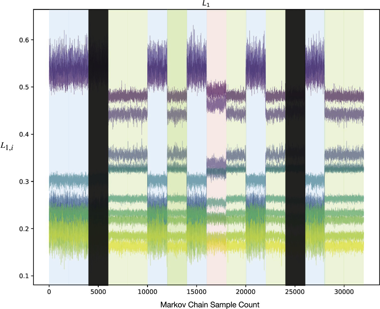
Figure 17. Posterior samplings for each of the L1 template's 10 components. The x-axis labels the 2000 samples for each of the 16 samplers, concatenated in sequence for 32,000 total draws. The aforementioned groupings are shaded blue, green, and pink. The dark gray rectangles mask the samples drawn by two samplers which became lost during sampling and were subsequently excluded from our analysis.
Download figure:
Standard image High-resolution imageTable 1. Model Per-supernova Parameter Median Values with 68th Percentile Upper and Lower Values
| SN | χ0 − 〈χ0〉 | s1 | c1 | c2 | t0 (MJD) |
|---|---|---|---|---|---|
| SNF 20060512-001 | − 0.04 ± 0.03 | −0.02 ± 0.01 | −0.33 ± 0.09 | 0.12 ± 0.03 | 53882.5 ± 0.12 |
| SNF 20060526-003 | −0.06 ± 0.03 | −0.07 ± 0.01 | −0.31 ± 0.09 | −0.04 ± 0.02 | 53893.4 ± 0.21 |
| SNF 20061020-000 | 0.30 ± 0.03 | 0.21 ± 0.01 | 0.44 ± 0.11 | 0.08 ± 0.03 | 54037.9 ± 0.19 |
| SNF 20061021-003 | −0.08 ± 0.03 | −0.05 ± 0.01 | 0.38 ± 0.08 | −0.04 ± 0.02 | 54039.7 ± 0.13 |
| SNF 20061022-005 | −0.11 ± 0.03 | −0.08 ± 0.02 | −0.34 ± 0.10 | 0.15 ± 0.03 | 54040.8 ± 0.17 |
| SNF 20061111-002 | 0.08 ± 0.03 | −0.01 ± 0.01 | −0.30 ± 0.12 | −0.05 ± 0.03 | 54060.8 ± 0.18 |
| SNF 20070424-003 | 0.08 ± 0.03 | −0.05 ± 0.01 | −0.26 ± 0.09 | −0.07 ± 0.02 | 54225.8 ± 0.16 |
| SNF 20070506-006 | −0.19 ± 0.03 | −0.07 ± 0.01 | −0.94 ± 0.08 | 0.09 ± 0.02 | 54245.9 ± 0.10 |
| SNF 20070630-006 | −0.09 ± 0.02 | −0.04 ± 0.01 | −0.16 ± 0.08 | −0.06 ± 0.02 | 54294.9 ± 0.11 |
| SNF 20070717-003 | −0.12 ± 0.02 | 0.03 ± 0.01 | 0.90 ± 0.08 | −0.12 ± 0.02 | 54310.3 ± 0.11 |
| SNF 20070802-000 | −0.19 ± 0.03 | −0.03 ± 0.01 | 1.00 ± 0.09 | −0.15 ± 0.02 | 54326.7 ± 0.13 |
| SNF 20070818-001 | −0.24 ± 0.03 | −0.04 ± 0.01 | 0.80 ± 0.10 | −0.16 ± 0.01 | 54339.0 ± 0.18 |
| SNF 20070831-015 | −0.28 ± 0.03 | −0.15 ± 0.01 | −0.23 ± 0.11 | −0.03 ± 0.03 | 54352.4 ± 0.26 |
| SNF 20070902-018 | 0.11 ± 0.03 | 0.08 ± 0.01 | 0.66 ± 0.10 | 0.04 ± 0.03 | 54353.2 ± 0.17 |
| SNF 20080507-000 | −0.30 ± 0.02 | −0.06 ± 0.01 | 0.44 ± 0.08 | 0.04 ± 0.02 | 54601.7 ± 0.16 |
| SNF 20080510-001 | −0.01 ± 0.03 | −0.05 ± 0.01 | −0.55 ± 0.08 | −0.05 ± 0.02 | 54607.5 ± 0.12 |
| SNF 20080510-005 | −0.00 ± 0.03 | −0.11 ± 0.01 | −0.75 ± 0.11 | −0.02 ± 0.03 | 54608.1 ± 0.18 |
| SNF 20080512-010 | 0.25 ± 0.03 | 0.16 ± 0.02 | −0.24 ± 0.09 | 0.12 ± 0.02 | 54603.9 ± 0.12 |
| SNF 20080514-002 | 0.50 ± 0.02 | 0.20 ± 0.01 | −0.73 ± 0.05 | 0.14 ± 0.01 | 54613.6 ± 0.06 |
| SNF 20080522-000 | −0.27 ± 0.02 | −0.08 ± 0.01 | −0.87 ± 0.08 | 0.20 ± 0.02 | 54624.3 ± 0.10 |
| SNF 20080522-011 | −0.11 ± 0.02 | −0.05 ± 0.01 | −1.02 ± 0.07 | −0.05 ± 0.02 | 54619.1 ± 0.12 |
| SNF 20080531-000 | 0.08 ± 0.02 | 0.05 ± 0.01 | 0.03 ± 0.07 | −0.08 ± 0.02 | 54625.9 ± 0.11 |
| SNF 20080614-010 | 0.24 ± 0.03 | 0.22 ± 0.01 | 0.55 ± 0.10 | 0.08 ± 0.03 | 54637.7 ± 0.10 |
| SNF 20080620-000 | 0.13 ± 0.03 | 0.09 ± 0.01 | 0.64 ± 0.10 | −0.03 ± 0.02 | 54642.7 ± 0.16 |
| SNF 20080626-002 | −0.16 ± 0.02 | −0.08 ± 0.01 | −0.47 ± 0.08 | −0.08 ± 0.02 | 54654.0 ± 0.15 |
| SNF 20080714-008 | −0.17 ± 0.02 | 0.00 ± 0.01 | 1.68 ± 0.07 | −0.20 ± 0.02 | 54670.0 ± 0.15 |
| SNF 20080725-004 | −0.07 ± 0.03 | −0.10 ± 0.01 | 0.05 ± 0.08 | −0.10 ± 0.02 | 54680.8 ± 0.20 |
| SNF 20080803-000 | −0.09 ± 0.03 | −0.05 ± 0.01 | 0.88 ± 0.10 | −0.04 ± 0.03 | 54693.1 ± 0.13 |
| SNF 20080810-001 | 0.17 ± 0.02 | 0.14 ± 0.01 | 0.10 ± 0.07 | 0.11 ± 0.02 | 54700.9 ± 0.08 |
| SNF 20080821-000 | −0.13 ± 0.02 | −0.06 ± 0.01 | −0.23 ± 0.08 | 0.01 ± 0.02 | 54710.1 ± 0.15 |
| SNF 20080825-010 | −0.04 ± 0.03 | 0.11 ± 0.01 | −0.20 ± 0.08 | 0.08 ± 0.02 | 54715.1 ± 0.10 |
| SNF 20080909-030 | −0.15 ± 0.05 | −0.04 ± 0.01 | −0.29 ± 0.17 | 0.05 ± 0.05 | 54733.8 ± 0.16 |
| SNF 20080913-031 | −0.19 ± 0.07 | 0.00 ± 0.02 | 0.55 ± 0.25 | −0.09 ± 0.07 | 54734.6 ± 0.40 |
| SNF 20080918-000 | −0.15 ± 0.03 | −0.11 ± 0.01 | 1.10 ± 0.11 | −0.09 ± 0.03 | 54736.8 ± 0.17 |
| CSS130502_01 | 0.29 ± 0.03 | −0.01 ± 0.01 | −1.23 ± 0.08 | 0.07 ± 0.02 | 56425.0 ± 0.14 |
| LSQ12fhe | −0.45 ± 0.03 | −0.07 ± 0.01 | −0.41 ± 0.12 | 0.22 ± 0.03 | 56214.9 ± 0.19 |
| LSQ14cnm | −0.00 ± 0.03 | −0.00 ± 0.01 | −0.88 ± 0.08 | −0.03 ± 0.02 | 56833.9 ± 0.14 |
| PTF09dlc | −0.00 ± 0.02 | −0.03 ± 0.01 | −0.56 ± 0.07 | −0.08 ± 0.02 | 55077.4 ± 0.13 |
| PTF09dnl | −0.23 ± 0.02 | −0.07 ± 0.01 | 0.26 ± 0.06 | −0.05 ± 0.02 | 55077.7 ± 0.16 |
| PTF09fox | 0.01 ± 0.02 | −0.08 ± 0.01 | −0.83 ± 0.07 | −0.05 ± 0.01 | 55135.8 ± 0.14 |
| PTF09foz | −0.06 ± 0.02 | 0.11 ± 0.01 | 0.48 ± 0.07 | −0.00 ± 0.02 | 55133.8 ± 0.11 |
| PTF10hmv | 0.11 ± 0.02 | −0.09 ± 0.01 | 1.04 ± 0.06 | −0.01 ± 0.02 | 55355.3 ± 0.11 |
| PTF10icb | 0.49 ± 0.02 | 0.01 ± 0.01 | 0.32 ± 0.07 | 0.03 ± 0.02 | 55363.7 ± 0.09 |
| PTF10mwb | 0.21 ± 0.02 | 0.10 ± 0.01 | 0.19 ± 0.06 | −0.02 ± 0.02 | 55392.6 ± 0.08 |
| PTF10nlg | 0.03 ± 0.02 | −0.03 ± 0.01 | 1.67 ± 0.07 | −0.20 ± 0.01 | 55394.8 ± 0.16 |
| PTF10qyz | 0.36 ± 0.03 | 0.10 ± 0.01 | −0.43 ± 0.10 | −0.08 ± 0.02 | 55429.0 ± 0.12 |
| PTF10wnm | −0.00 ± 0.02 | −0.09 ± 0.01 | −0.66 ± 0.08 | 0.03 ± 0.02 | 55480.5 ± 0.17 |
| PTF10wof | 0.02 ± 0.03 | −0.06 ± 0.01 | 0.12 ± 0.10 | −0.12 ± 0.02 | 55476.7 ± 0.28 |
| PTF11bgv | 0.22 ± 0.03 | 0.03 ± 0.01 | 0.30 ± 0.08 | 0.14 ± 0.02 | 55645.6 ± 0.12 |
| PTF11bju | −0.23 ± 0.03 | −0.05 ± 0.01 | −0.14 ± 0.09 | 0.26 ± 0.02 | 55652.7 ± 0.14 |
| PTF11bnx | −0.00 ± 0.03 | 0.03 ± 0.01 | 1.44 ± 0.09 | −0.16 ± 0.02 | 55655.6 ± 0.16 |
| PTF11mkx | −0.50 ± 0.04 | −0.00 ± 0.01 | −0.33 ± 0.13 | 0.27 ± 0.02 | 55837.8 ± 0.10 |
| PTF11mty | −0.04 ± 0.02 | −0.07 ± 0.01 | −0.82 ± 0.08 | 0.02 ± 0.02 | 55840.2 ± 0.12 |
| PTF12dxm | 0.34 ± 0.03 | 0.22 ± 0.01 | 0.89 ± 0.09 | 0.02 ± 0.02 | 56054.8 ± 0.09 |
| PTF12fuu | 0.18 ± 0.02 | −0.05 ± 0.01 | −451.28 ± 0.07 | 0.01 ± 0.02 | 56115.2 ± 0.09 |
| PTF12grk | 0.10 ± 0.03 | 0.12 ± 0.01 | 0.77 ± 0.10 | −0.16 ± 0.01 | 56137.0 ± 0.10 |
| PTF12iiq | 0.07 ± 0.04 | 0.12 ± 0.01 | 1.17 ± 0.13 | −0.17 ± 0.02 | 56183.6 ± 0.16 |
| PTF13anh | −0.09 ± 0.03 | 0.05 ± 0.01 | 0.51 ± 0.12 | −0.15 ± 0.01 | 56416.1 ± 0.16 |
| SN 2004ef | 0.07 ± 0.02 | 0.14 ± 0.01 | 1.28 ± 0.06 | −0.08 ± 0.02 | 53265.0 ± 0.08 |
| SN 2005hc | 0.00 ± 0.03 | −0.07 ± 0.01 | −0.61 ± 0.09 | −0.03 ± 0.02 | 53670.5 ± 0.18 |
| SN 2005hj | −0.23 ± 0.03 | −0.13 ± 0.01 | −0.57 ± 0.09 | 0.11 ± 0.02 | 53677.9 ± 0.23 |
| SN 2006cj | 0.02 ± 0.02 | −0.06 ± 0.01 | −0.84 ± 0.06 | 0.04 ± 0.02 | 53882.4 ± 0.11 |
| SN 2007bd | 0.16 ± 0.03 | 0.03 ± 0.02 | −0.58 ± 0.10 | −0.02 ± 0.02 | 54207.6 ± 0.16 |
| SN 2010dt | 0.03 ± 0.03 | 0.00 ± 0.01 | −0.44 ± 0.09 | −0.10 ± 0.01 | 55363.4 ± 0.11 |
| SN 2011bc | −0.05 ± 0.02 | 0.04 ± 0.01 | 1.18 ± 0.08 | −0.05 ± 0.02 | 55669.6 ± 0.15 |
| SN 2011be | 0.22 ± 0.03 | −0−0.03 ± 0.01 | −1.20 ± 0.08 | 0.08 ± 0.02 | 55656.9 ± 0.12 |
| SN 2011ga | 0.05 ± 0.02 | 0.02 ± 0.01 | −0.43 ± 0.08 | −0.03 ± 0.02 | 55832.7 ± 0.13 |
| SN 2011gf | 0.07 ± 0.03 | −0.07 ± 0.01 | −1.54 ± 0.07 | −0.04 ± 0.01 | 55833.5 ± 0.12 |
| SN 2011hr | −0.25 ± 0.03 | −0.03 ± 0.01 | 0.12 ± 0.08 | 0.25 ± 0.02 | 55891.0 ± 0.10 |
| SN 2012cg | 0.63 ± 0.02 | 0.00 ± 0.01 | 0.67 ± 0.07 | 0.05 ± 0.02 | 56084.5 ± 0.10 |
| SN 2012dn | −0.08 ± 0.03 | −0.03 ± 0.01 | 0.23 ± 0.09 | 0.20 ± 0.02 | 56135.1 ± 0.06 |
| SN 2012fr | −0.56 ± 0.02 | −0.09 ± 0.01 | −0.60 ± 0.05 | −0.09 ± 0.01 | 56247.1 ± 0.05 |
| SN 2013bt | 0.40 ± 0.04 | 0.22 ± 0.01 | −0.28 ± 0.11 | 0.12 ± 0.03 | 56411.4 ± 0.11 |
Note. Per-SN parameters χ0 − 〈χ0〉, s1, c1, and c2 have been transformed to magnitudes. The parameter t0 is the date corresponding to maximum-phase node of the light-curve model for the third band centered at 4084 Å.
Footnotes
- 23
The use of GPMPs over other techniques (e.g., spline interpolation) is partly historical. Our original intention was to treat model functions probabilistically, a use for which Gaussian processes would have been suited. We later opted to use the more conventional approach of using a deterministic function as is done in SALT2.
- 24
The unit vector constraints for L1, L2, and M1 are what prevent these templates from being described as color variation templates. If instead we constrained these templates at a reference wavelength node to be fixed to zero, then these templates would have units color, per the usual astronomical definition.
- 25
- 26
In general, a plane is an affine space, not a vector space. All planes described in this paper do pass through the embedding vector space's origin, which ensures they are proper 2D vector subspaces. Because of this, all planes discussed either intersect or are parallel. For brevity, in this paper we refer to any 2D subspaces as planes.
- 27
We developed this technique and are not aware of any previous equivalent use.
- 28
159 from F0, 159 from M1, nine from L1, and nine from L2, specifically.
- 29