Abstract
We present an analysis of oscillation mode variability in the hot B subdwarf star EPIC 220422705, a new pulsator discovered from ∼78 days of K2 photometry. The high-quality light curves provide a detection of 66 significant independent frequencies, from which we identified nine incomplete potential triplets and three quintuplets. Those g- and p-multiplets give rotation periods of ∼36 and 29 days in the core and at the surface, respectively, potentially suggesting a slightly differential rotation. We derived a period spacing of 268.5 s and 159.4 s for the sequence of dipole and quadrupole modes, respectively. We characterized the precise patterns of amplitude and frequency modulations (AM and FM) of 22 frequencies with high enough amplitude for our science. Many of them exhibit intrinsic and periodic patterns of AM and FM, with periods on a timescale of months as derived by the best fitting and Markov Chain Monte Carlo test. The nonlinear resonant mode interactions could be a natural interpretation for such AMs and FMs after other mechanisms are ruled out. Our results are the first step to building a bridge between mode variability from K2 photometry and the nonlinear perturbation theory of stellar oscillation.
Original content from this work may be used under the terms of the Creative Commons Attribution 4.0 licence. Any further distribution of this work must maintain attribution to the author(s) and the title of the work, journal citation and DOI.
1. Introduction
Hot B subdwarf (sdB) stars burn helium in the core and are typically wrapped in a thin hydrogen envelope at the surface. Their compact ( dex) and hot (Teff = 20,000 ∼ 40,000 K) properties place them in the extreme horizontal branch (EHB) in the Hertzsprung–Russell diagram (see Heber 2009, 2016, for a review). A fraction of those blue faint objects have luminosity variations which can be attributed to oscillations of gravity (g-) or pressure (p-) modes or both (Green et al. 2003; Kilkenny et al. 1997; Schuh et al. 2006). Those modes are driven by the classical κ-mechanism due to an opacity bump produced by the ionization of iron group elements (Charpinet et al. 1996, 1997; Fontaine et al. 2003). Due to their rich oscillations, sdB variables (sdBV) are good candidates to probe their interior via the tool of asteroseismology (Charpinet et al. 2005).
As advanced by observations from space, for instance, Kepler/K2 and TESS (Borucki et al. 2010; Howell et al. 2014; Ricker et al. 2015) oscillation frequencies in sdBV stars can be sharply resolved to unprecedented high precision, which leads to fruitful achievements for probing the interior of sdB stars (see, e.g., Van Grootel et al. 2010; Reed et al. 2014; Charpinet et al. 2019). There are 18 sdBV stars discovered in the original Kepler field (Østensen et al. 2010, 2011; Pablo et al. 2011; Reed et al. 2012), among which most stars were continuously observed after they were discovered to pulsate. In contrast to ground-based photometry, several sdBV stars are found with more than 100 frequencies, such as KIC 03527751 (Foster et al. 2015; Zong et al. 2018). A preliminary mass survey on sdBV stars established that they are distributed around the canonical value ∼0.47 M⊙ in a narrow region (Fontaine et al. 2012) with rotational periods distributed from a few days up to even hundreds of days (Charpinet et al. 2018; Reed et al. 2021; Silvotti et al. 2021). In individual analyses, many sdBVs show clear variations in amplitude with a timescale much longer than their oscillation periods (Reed et al. 2014; Zong et al. 2016a; Kern et al. 2017). Focusing on amplitude modulations, Zong et al. (2016a) found that frequencies are not stable for many rotational components in KIC 10139564. They concluded that the amplitude and frequency modulations (AM/FM) could be attributed to nonlinear interactions of resonant mode coupling (Goupil & Buchler 1994; Buchler et al. 1995, 1997), a mechanism of intense focus in other pulsators, for instance, pulsating white dwarfs (Zong et al. 2016b) and slowly pulsating B stars (Van Beeck et al. 2021). Observational AM/FM variations provide strong constraints for the development of nonlinear stellar oscillation theory.
However, the Kepler space telescope had to begin the reborn mission with pointing using only two reaction wheels. This so-called K2 phase provided nearly uninterrupted photometry for almost 3 months but could observe a larger spatial coverage than the original Kepler mission. Therefore, K2 offers a higher chance of finding more sdBV stars. In the 20 campaigns of K2, nearly 200 sdBV candidates were observed to search for pulsations or transits, leading to 10 sdBV stars already published (see, e.g., Reed et al. 2019; Baran et al. 2019; Silvotti et al. 2019). These ∼80 days K2 observations could also be helpful for characterizing the amplitude modulations of pulsation modes in sdBVs (see, e.g., Silvotti et al. 2019). Similar to Kepler results, K2 photometry will shed new light on AM/FM oscillations in sdBV stars on shorter-term timescales.
As demonstrated by a series of works from Zong et al. (2016a, 2016b, 2018), evolved compact pulsators, including pulsating white dwarfs and sdBVs, could be excellent candidates for providing observational constraints for developing the nonlinear amplitude equations that describe how amplitudes and frequencies modulate. Gained from those experiences, we initiated a new survey of AM/FM in sdBV stars from K2 on relatively shorter modulation timescales appropriate for K2. In this paper, we concentrate on the bright sdB star, EPIC 220422705, or PG 0039+049, which has Kp
= 12.875 and is located at α = 00h42m06124 and δ = + 05d09m23
376. This star was originally identified as a faint blue star by Berger & Fringant (1980) and then was classified as an sdB star with spectra (Kilkenny et al. 1988). Moehler et al. (1990) derived atmospheric parameters of Teff = 26700 K and
 dex for EPIC 220422705, with a distance of d = 1050 ± 400 pc and refined by GAIA EDR3 to
  pc (Gaia Collaboration et al. 2021). It is a binary system containing a cool companion, as disclosed by Copperwheat et al. (2011), and further confirmed as a G2V dwarf star with a preliminary period of 150–300 (±220) days (Barlow et al. 2012). The structure of the paper is organized as follows: we analyze the photometric data from K2 and analyze the asteroseismic properties in Section 2. We then characterized the amplitude and frequency modulations of 22 frequencies in Section 3, followed by a discussion of those modulation details in Section 4. Finally, we summarize our findings in Section 5.
2. Frequency Content
2.1. Photometry and Frequency Extraction
EPIC 220422705 had been observed by K2 in short-cadence (SC) mode over a period of 78.72 days during Campaign 8. Its assembled light curves were downloaded from Mikulski Archive for Space Telescopes 7 (MAST). These archived data were processed through the EPIC Variability Extraction and Removal for Exoplanet Science Targets (EVEREST) pipeline. 8 The photometry corrected by EVEREST has comparable precision to the original Kepler mission for targets brighter than Kp ≈ 13 (Luger et al. 2018). EPIC 220422705 is within this brightness range.
The EVEREST flux was first shifted to the relative fraction of their mean value. We then used a sixth-order polynomial fitting to detrend the whole light curve due to residual instrumental drifts. To avoid discontinuities in the light curve across gaps longer than 0.02 days, we separated the light curve piecewise where such gaps occurred for our fitting. This detrending method will flatten the light curves and dismiss signals with a period (≳2 days) in Fourier transform, which will not have an impact on the modulating patterns for our prime aim. We note that those signals are not concerned here due to the fact that the EVEREST pipeline may not recover those signals correctly. Then the light curves were iteratively clipped of a few outliers three times by filtering at 4.5σ around the light curve before we produced a Fourier transformation. Figure 1 (top panel) shows the final light curve of EPIC 220422705, which contains 106,444 data points over a duration of 76.43 days with a 1.2 days gap in the middle. The amplitude scatter clearly reveals multiperiodic signals of hours in a close-up view (middle panel). The corresponding Lomb–Scargle periodogram (LSP; Lomb 1976; Scargle 1982) up to the Nyquist frequency is shown in the bottom panel where the g-mode frequencies are clearly dominant in a region of [∼100–1000] μHz.
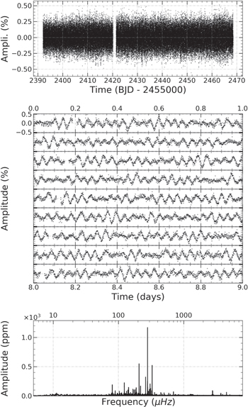
Figure 1. K2 photometry and frequency signals obtained for EPIC 220422705. Top panel: the complete light curve (amplitude is the percentage of the mean brightness) with a data sampling of 58.85 s. Middle panel: a close-up view of a 9 day light curve (starting at BJD 2457433) with each panel having a one-day slice. Bottom panel: the Lomb–Scargle periodogram of the assembled light curve (amplitude in ppm vs. frequency in μHz on a logarithmic scale).
Download figure:
Standard image High-resolution imageWe used the specialized software FELIX 9 to perform frequency extraction from the light curves. The frequencies were prewhitened in order of decreasing amplitude until the value of 5.2 times the local noise level, a value that is the median amplitude in the LSP (Zong et al. 2021). This detection threshold is adopted as a compromise between 2 yr Kepler and 27 days of TESS photometry (Zong et al. 2016b; Charpinet et al. 2019). The highest peak will be extracted in the case where there are several close frequencies of <0.4 μHz, i.e., about 3 × Δf (Δf = 1/T, and T ∼76.43 days). We have detected 66 independent frequencies and 13 linear combination frequencies, with the highest (1172 ppm) frequency at 279.767 μHz, which are listed in Table 1.
Table 1. All Frequencies Above the 5.2σ Threshold Detected in EPIC 220422705, by Order of Increasing Frequency
| ID | Frequency | σf | Period | σP | Amplitude | σA | S/N | ℓ | nl=1 | nl=2 | Comments |
|---|---|---|---|---|---|---|---|---|---|---|---|
| (μHz) | (μHz) | (s) | (s) | (ppm) | (ppm) | ||||||
| f36 | 78.513718 | 0.013490 | 12736.627704 | 2.188323 | 48.530 | 7.840 | 6.2 | 1/2 | 41 | 71 | ⋯ |
| f07 | 80.593286 | 0.003472 | 12407.981531 | 0.534585 | 190.710 | 7.930 | 24.0 | 2 | ⋯ | 69 | AFM |
| f47 | 81.745528 | 0.015576 | 12233.085076 | 2.330880 | 42.300 | 7.890 | 5.4 | 1/2 | 39 | 68 | ⋯ |
| * f18 | 89.477815 | 0.007410 | 11175.954576 | 0.925537 | 89.440 | 7.940 | 11.3 | 2 | ⋯ | 61 | ⋯ |
| f46 | 97.679239 | 0.015759 | 10237.590017 | 1.651719 | 42.470 | 8.020 | 5.3 | 2 | ⋯ | 55 | ⋯ |
| f22 | 103.303172 | 0.008272 | 9680.244884 | 0.775105 | 81.070 | 8.030 | 10.1 | 1 | 30 | ⋯ | ⋯ |
| f44 | 105.886042 | 0.015751 | 9444.115392 | 1.404888 | 42.790 | 8.070 | 5.3 | 2 | ⋯ | 50 | ⋯ |
| f32 | 112.125753 | 0.012740 | 8918.557707 | 1.013372 | 52.680 | 8.040 | 6.6 | 1/2 | 27 | 47 | ⋯ |
| * f05 | 123.087962 | 0.002951 | 8124.271307 | 0.194805 | 225.750 | 7.980 | 28.3 | 1 | 24 | ⋯ | AFM |
| f26 | 123.938687 | 0.010759 | 8068.505692 | 0.700420 | 61.000 | 7.860 | 7.8 | ⋯ | ⋯ | ⋯ | ⋯ |
| f42 | 129.430699 | 0.014990 | 7726.142304 | 0.894816 | 43.060 | 7.730 | 5.6 | ⋯ | ⋯ | ⋯ | ⋯ |
| f21 | 133.290520 | 0.007839 | 7502.409023 | 0.441213 | 81.810 | 7.680 | 10.7 | 1/2 | 22 | 38 | ⋯ |
| f16 | 139.917867 | 0.006231 | 7147.050042 | 0.318290 | 101.460 | 7.570 | 13.4 | 2 | ⋯ | 36 | AFM |
| f09 | 143.418651 | 0.004274 | 6972.593805 | 0.207766 | 146.640 | 7.510 | 19.5 | 1/2 | 20 | 35 | AFM |
| f28 | 153.730694 | 0.010519 | 6504.881834 | 0.445117 | 58.670 | 7.390 | 7.9 | 2 | ⋯ | 32 | ⋯ |
| f48 | 159.361976 | 0.014897 | 6275.022613 | 0.586567 | 40.200 | 7.170 | 5.6 | ⋯ | ⋯ | ⋯ | ⋯ |
| f12 | 166.836670 | 0.005122 | 5993.886121 | 0.184000 | 116.840 | 7.170 | 16.3 | 1/2 | 16 | 29 | AFM |
| f15 | 173.403913 | 0.005551 | 5766.882542 | 0.184615 | 103.960 | 6.910 | 15.0 | ⋯ | ⋯ | ⋯ | AFM |
| * f14 | 180.391866 | 0.005258 | 5543.487202 | 0.161575 | 106.320 | 6.700 | 15.9 | 1 | 14 | AFM | |
| f34 | 183.040112 | 0.011008 | 5463.283371 | 0.328564 | 49.530 | 6.530 | 7.6 | ⋯ | × | ⋯ | ⋯ |
| f10 | 187.474901 | 0.003790 | 5334.047369 | 0.107838 | 141.280 | 6.410 | 22.0 | ⋯ | ⋯ | ⋯ | AFM |
| f25 | 189.829069 | 0.008628 | 5267.897084 | 0.239427 | 62.020 | 6.410 | 9.7 | ⋯ | ⋯ | ⋯ | ⋯ |
| f40 | 191.060597 | 0.012136 | 5233.941562 | 0.332457 | 43.830 | 6.370 | 6.9 | 2 | ⋯ | 24 | ⋯ |
| * f41 | 198.891984 | 0.012027 | 5027.854728 | 0.304024 | 43.560 | 6.270 | 6.9 | 1 | 12 | ⋯ | ⋯ |
| f31 | 203.922726 | 0.009663 | 4903.818333 | 0.232369 | 53.600 | 6.200 | 8.6 | 2 | ⋯ | 22 | ⋯ |
| f02 | 207.239959 | 0.000919 | 4825.324262 | 0.021389 | 555.800 | 6.120 | 90.9 | ⋯ | ⋯ | ⋯ | AFM |
| f56 | 213.023531 | 0.015460 | 4694.317078 | 0.340689 | 32.410 | 6.000 | 5.4 | ⋯ | ⋯ | ⋯ | ⋯ |
| f08 | 218.362945 | 0.002993 | 4579.531562 | 0.062779 | 166.040 | 5.950 | 27.9 | 2 | ⋯ | 20 | AFM |
| f57 | 237.295070 | 0.015685 | 4214.162557 | 0.278551 | 30.530 | 5.740 | 5.3 | ⋯ | ⋯ | ⋯ | ⋯ |
| f04 | 261.267965 | 0.001401 | 3827.488003 | 0.020527 | 326.870 | 5.490 | 59.6 | 1/2 | 8 | 15 | AFM |
| f01 | 279.767107 | 0.000388 | 3574.401619 | 0.004957 | 1172.450 | 5.450 | 215.2 | ⋯ | × | ⋯ | AFM |
| f51 | 281.531170 | 0.012426 | 3552.004566 | 0.156770 | 36.490 | 5.430 | 6.7 | ⋯ | ⋯ | ⋯ | ⋯ |
| * f23 | 288.561685 | 0.005718 | 3465.463543 | 0.068675 | 80.340 | 5.500 | 14.6 | 1 | 7 | ⋯ | AFM |
| f13 | 299.038501 | 0.003969 | 3344.051003 | 0.044386 | 110.410 | 5.250 | 21.0 | 2 | ⋯ | 12 | AFM |
| f37 | 299.821635 | 0.009171 | 3335.316351 | 0.102016 | 47.790 | 5.250 | 9.1 | ⋯ | ⋯ | ⋯ | ⋯ |
| f06 | 306.222893 | 0.002015 | 3265.595173 | 0.021489 | 208.080 | 5.020 | 41.4 | 1 | 6 | ⋯ | AFM |
| f11 | 311.999395 | 0.003205 | 3205.134420 | 0.032923 | 128.280 | 4.920 | 26.1 | ⋯ | ⋯ | ⋯ | AFM |
| * f19 | 324.165036 | 0.004423 | 3084.848419 | 0.042093 | 89.190 | 4.730 | 18.9 | 1 | 5 | ⋯ | AFM |
| f03 | 328.746189 | 0.000716 | 3041.860354 | 0.006628 | 529.150 | 4.540 | 116.5 | 2 | ⋯ | 10 | AFM |
| f27 | 358.059551 | 0.005609 | 2792.831516 | 0.043749 | 60.530 | 4.070 | 14.9 | ⋯ | ⋯ | ⋯ | ⋯ |
| f29 | 447.460239 | 0.005372 | 2234.835441 | 0.026831 | 56.730 | 3.650 | 15.5 | 1/2 | 2 | 5 | ⋯ |
| f50 | 466.933411 | 0.007938 | 2141.632997 | 0.036406 | 37.600 | 3.570 | 10.5 | ⋯ | ⋯ | ⋯ | ⋯ |
| * f30 | 501.251468 | 0.005673 | 1995.006626 | 0.022580 | 54.020 | 3.670 | 14.7 | 1 | 1 | ⋯ | ⋯ |
| f35 | 590.545320 | 0.006904 | 1693.350139 | 0.019798 | 48.610 | 4.020 | 12.1 | 1 | 0 | ⋯ | ⋯ |
| f66 | 591.095424 | 0.013287 | 1691.774221 | 0.038028 | 25.300 | 4.030 | 6.3 | ⋯ | ⋯ | ⋯ | ⋯ |
| * f54 | 622.788529 | 0.010358 | 1605.681470 | 0.026705 | 32.650 | 4.050 | 8.1 | 2 | ⋯ | 1 | ⋯ |
| * f24 | 697.626978 | 0.004600 | 1433.430803 | 0.009453 | 71.660 | 3.950 | 18.1 | 2 | ⋯ | 0 | AFM |
| f53 | 698.271310 | 0.009803 | 1432.108101 | 0.020105 | 33.660 | 3.950 | 8.5 | ⋯ | ⋯ | ⋯ | ⋯ |
| f55 | 698.742459 | 0.010012 | 1431.142457 | 0.020507 | 32.600 | 3.910 | 8.3 | ⋯ | ⋯ | ⋯ | ⋯ |
| f78 | 738.045426 | 0.015618 | 1354.930150 | 0.028672 | 20.240 | 3.790 | 5.3 | ⋯ | ⋯ | ⋯ | ⋯ |
| f64 | 745.027287 | 0.011907 | 1342.232717 | 0.021451 | 26.370 | 3.760 | 7.0 | ⋯ | ⋯ | ⋯ | ⋯ |
| f61 | 835.597738 | 0.012233 | 1196.748093 | 0.017520 | 26.870 | 3.940 | 6.8 | ⋯ | ⋯ | ⋯ | ⋯ |
| f70 | 977.688720 | 0.013094 | 1022.820434 | 0.013699 | 23.660 | 3.710 | 6.4 | ⋯ | ⋯ | ⋯ | ⋯ |
| f68 | 1250.082073 | 0.012890 | 799.947477 | 0.008249 | 24.200 | 3.740 | 6.5 | ⋯ | ⋯ | ⋯ | ⋯ |
| f59 | 1263.268911 | 0.011052 | 791.597095 | 0.006925 | 28.960 | 3.830 | 7.6 | ⋯ | ⋯ | ⋯ | ⋯ |
| f73 | 1280.609422 | 0.014074 | 780.878216 | 0.008582 | 22.930 | 3.860 | 5.9 | ⋯ | ⋯ | ⋯ | ⋯ |
| f67 | 1293.989776 | 0.013128 | 772.803633 | 0.007840 | 24.410 | 3.840 | 6.4 | ⋯ | ⋯ | ⋯ | ⋯ |
| f63 | 1315.516923 | 0.011645 | 760.157458 | 0.006729 | 26.450 | 3.690 | 7.2 | ⋯ | ⋯ | ⋯ | ⋯ |
| f76 | 1339.686713 | 0.014558 | 746.443172 | 0.008111 | 21.080 | 3.680 | 5.7 | ⋯ | ⋯ | ⋯ | ⋯ |
| f79 | 2702.635472 | 0.013530 | 370.009204 | 0.001852 | 20.170 | 3.270 | 6.2 | ⋯ | ⋯ | ⋯ | ⋯ |
| f17 | 2768.529437 | 0.003033 | 361.202589 | 0.000396 | 89.530 | 3.250 | 27.5 | ⋯ | ⋯ | ⋯ | AFM |
| f20 | 2781.657771 | 0.003223 | 359.497854 | 0.000417 | 86.390 | 3.330 | 25.9 | ⋯ | ⋯ | ⋯ | AFM |
| f69 | 2829.666372 | 0.011498 | 353.398553 | 0.001436 | 24.150 | 3.330 | 7.3 | ⋯ | ⋯ | ⋯ | ⋯ |
| * f52 | 3706.124351 | 0.009301 | 269.823650 | 0.000677 | 34.070 | 3.800 | 9.0 | 1 | ⋯ | ⋯ | ⋯ |
| * f39 | 3720.773872 | 0.006863 | 268.761294 | 0.000496 | 45.960 | 3.780 | 12.2 | 1 | ⋯ | ⋯ | AFM |
| * f62 | 3741.962308 | 0.011572 | 267.239464 | 0.000826 | 26.740 | 3.710 | 7.2 | 1 | ⋯ | ⋯ | ⋯ |
| Combination Frequencies | |||||||||||
| f38 | 95.909702 | 0.014504 | 10426.473881 | 1.576715 | 46.290 | 8.040 | 5.8 | ⋯ | ⋯ | ⋯ | f37 − f31 |
| f45 | 98.046119 | 0.015753 | 10199.281873 | 1.638675 | 42.570 | 8.030 | 5.3 | ⋯ | ⋯ | ⋯ | f31 − f44 |
| f33 | 110.348492 | 0.013488 | 9062.199093 | 1.107641 | 50.150 | 8.100 | 6.2 | ⋯ | ⋯ | ⋯ | f3 − f8 |
| f43 | 148.317644 | 0.014488 | 6742.286152 | 0.658587 | 42.970 | 7.460 | 5.8 | ⋯ | ⋯ | ⋯ | f3 − f14 |
| f49 | 232.563301 | 0.012359 | 4299.904569 | 0.228515 | 38.320 | 5.670 | 6.8 | ⋯ | ⋯ | ⋯ | 1/3f24 |
| f59 | 326.972087 | 0.014200 | 3058.365043 | 0.132823 | 26.940 | 4.580 | 5.9 | ⋯ | ⋯ | ⋯ | 4f47 |
| f57 | 388.249071 | 0.010933 | 2575.666174 | 0.072529 | 29.350 | 3.840 | 7.6 | ⋯ | ⋯ | ⋯ | 3f42 |
| f73 | 587.586784 | 0.015314 | 1701.876263 | 0.044356 | 21.950 | 4.030 | 5.5 | ⋯ | ⋯ | ⋯ | f23 + f13 |
| f70 | 764.253882 | 0.013222 | 1308.465713 | 0.022638 | 23.550 | 3.730 | 6.3 | ⋯ | ⋯ | ⋯ | 4f40 |
| f76 | 1330.731963 | 0.014910 | 751.466131 | 0.008419 | 20.490 | 3.660 | 5.6 | ⋯ | ⋯ | ⋯ | f7 + f68 |
| f64 | 1343.875889 | 0.011808 | 744.116334 | 0.006538 | 25.620 | 3.620 | 7.1 | ⋯ | ⋯ | ⋯ | f7 + f59 |
| f71 | 1374.605015 | 0.012746 | 727.481705 | 0.006746 | 23.050 | 3.520 | 6.6 | ⋯ | ⋯ | ⋯ | f7 + f67 |
| f74 | 1396.135693 | 0.013454 | 716.262757 | 0.006902 | 21.530 | 3.470 | 6.2 | ⋯ | ⋯ | ⋯ | f7 + f63 |
Note. Column (1) The identification (ID in order of decreasing amplitude). (2) and (3) List frequencies in μHz and errors. (4) and (5) Periods in seconds and errors. (6) and (7) Amplitudes in ppm (parts per million) and errors. (8) Signal-to-noise ratio (S/N) above the local noise level. (9)–(11) The quantum number identified by the asymptotic regime (see Section 2.4). (12) Comments on whether amplitude or frequency modulations were explored or not. AM/FM/AFM indicates that the frequency has a modulation of amplitude (AM), frequency (FM), or both (AFM). “×” means the mode identified with period spacing but close to the value identified with potential splitting frequencies.
2.2. p and g Modes
Pulsating stars with both acoustic p-mode oscillations and gravity g-mode oscillations are excellent candidates to probe their internal profiles since acoustic and gravity waves propagate in different regions of the stellar structure (Aerts et al. 2010; Kurtz 2022). From spaceborne photometry, some g-mode-dominated sdBVs are found with low-amplitude p-mode pulsations (see, e.g., Baran et al. 2017; Zong et al. 2018; Sahoo et al. 2020). A direct and easy way to distinguish the two different types of modes is by their pulsation period. In general, theoretical sdB star calculations suggest that dipole p-modes typically have frequency >2500 μHz (P < 400 s), whereas g-modes <1000 μHz (P > 1000 s) (Fontaine et al. 2003; Charpinet et al. 2005, 2011). But p-mode frequencies can decrease below 1700 μHz (periods can increase beyond 600 s) as Teff and  decreases (Charpinet 1999; Charpinet et al. 2001, 2002).
Figure 2 shows preliminary classification for the p- and g-mode regions based only on the period. We detect 53 independent frequencies in the range [∼80–1000] μHz, which are clearly g-mode (P > 1000 s) pulsations (top two panels). Another seven independent frequencies are found in the high-frequency p-mode (P < 400 s) region, [∼2600–3800] μHz (bottom panel). There are six independent frequencies in the region of [∼1100–1400] μHz or [∼715–910] s, which might be low-order high-degree (ℓ > 3) g-modes or mixed modes that need further classification (see, e.g., Charpinet et al. 2011, 2019). Those frequencies, hardly directly classified to be p or g mode by merely their frequency value, can be used to penetrate a much larger portion of stellar interior or to detect the differential rotation in radial or longitude. However, determining the exact modes requires an exploration of seismic models. We note that a few frequencies were detected in this intermediate region in sdB stars observed with Kepler photometry; for instance, KIC 3527751 and KIC 10001893 (Foster et al. 2015; Uzundag et al. 2017). In addition, we have resolved 13 linear combinations with frequencies >1400 μHz, which could be intrinsic resonant modes (Zong et al. 2016a) or nonlinear effects from the linear eigenfrequencies (Brassard et al. 1995).
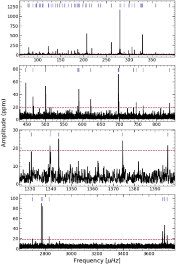
Figure 2. Close-up views of the LSP of EPIC 220422705. The entire periodogram is divided into two different ranges: the low-frequency g-mode region (top two panels) and the high-frequency p-mode region (bottom two panels). The horizontal dashed line denotes the 5.2σ detection threshold and the (blue) vertical segments at the top of each panel indicate the locations of extracted frequencies.
Download figure:
Standard image High-resolution image2.3. Rotational Multiplets
From linear perturbation theory, an eigenmode of oscillation can be characterized by spherical harmonics that are described by three quantum numbers: the radial order n, the degree ℓ, and the azimuthal order m. When a star rotates, the degenerated m components will split into 2ℓ + 1 multiplets. Referring to Ledoux (1951), their frequencies are related by,

where νn,l,0 is the frequency of the central m = 0 component, Ω is the solid rotational frequency, and Cn,ℓ is the Ledoux constant. For acoustic p mode, Cn,ℓ is very near to zero and can be ignored, whereas it is estimated as Cn,ℓ ∼ 1/ℓ(ℓ + 1) for high-radial order gravity g modes.
To resolve any rotational split multiplet from spaceborne photometry, a minimum criterion is that the observations should cover at least twice the rotation periods. Charpinet et al. (2018) and Silvotti et al. (2021) present the distribution of rotation periods for sdB stars determined from Kepler photometry. Frequency multiplets found rotation periods from a few days to near 1 yr, with most having periods a bit longer than 1 month. This indicates that K2 photometry can likely resolve frequency multiplets in sdB stars.
Figure 3 shows the frequency spacings of 12 groups of frequencies. We first consider six g-mode frequency groups that are detected with close frequency spacings around 0.17 μHz, which we consider to be dipole modes, i.e., f5 ∼ 123.09 μHz, f14 ∼ 180.39 μHz, f41 ∼ 198.89 μHz, f23 ∼ 288.56 μHz, f19 ∼ 324.16 μHz, and f30 ∼ 501.25 μHz. The weighted (by 1/σ fi ) average value is 0.168 ± 0.016 μHz. Those dipole modes give a rotational frequency of 0.33 μHz, which would mean quintuplet splitting of 0.28 μHz using Cn,1 = 1/2 and Cn,2 = 1/6. Three g-modes, f18 ∼ 89.48 μHz, f54 ∼ 622.79 μHz, and f24 ∼ 697.63 μHz, have close frequency spacings of ∼0.23 μHz, which could be rotational quintuplets, considering frequency uncertainties. We also resolve three ℓ = 1 p-mode multiplets, f52 ∼ 3706.12 μHz, f39 ∼ 3720.77 μHz, and f62 ∼ 3741.96 μHz, with low-amplitude peaks at a frequency distance of ∼0.4 μHz.
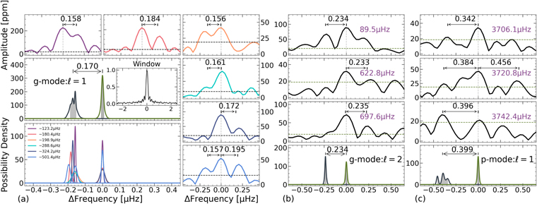
Figure 3. Likely multiplet frequencies induced by rotation detected in EPIC 220422705. (a) Six g-mode triplet components. The multiplets are shown in the top and right panels, with the horizontal lines indicating the 5.2σ threshold, and the frequency spacings are given in each panel. Different frequencies are marked by their colors provided in the bottom-left panel, where each Gaussian distribution represents the probability density of a component by their shifted frequency and error. In the middle-left panel, the superposition function of all components gives the probability density of frequency spacing, and the area in shadow defines the probability of 68.27%, which is identical to 1σ of N ∼ (0, 1). (b) Similar to (a) but for three incomplete g-mode quintuplets. (c) Similar to (a) but for three p-mode triplet components.
Download figure:
Standard image High-resolution imageIn order to determine the rotational period in a quantitative way, we propose a new approach that defines the rotation period associated with errors by their probability of occurrence. As shown in Figure 3, we adopt a Gaussian distribution,  , to represent the probability of a group of resolved frequencies at their shifted values. Here δ
fi
is the relative frequency to the central component. The probability of 68.27% (i.e., 1σ in N ∼ (0, 1)) was calculated to define the values and the uncertainties of frequency spacings. We obtained the values of 0.170 ± 0.049 μHz, 0.234 ± 0.035 μHz, and 0.399 ± 0.132 μHz for ℓ = 1, and 2 g modes and p modes, respectively. The corresponding rotation periods are
, to represent the probability of a group of resolved frequencies at their shifted values. Here δ
fi
is the relative frequency to the central component. The probability of 68.27% (i.e., 1σ in N ∼ (0, 1)) was calculated to define the values and the uncertainties of frequency spacings. We obtained the values of 0.170 ± 0.049 μHz, 0.234 ± 0.035 μHz, and 0.399 ± 0.132 μHz for ℓ = 1, and 2 g modes and p modes, respectively. The corresponding rotation periods are  ,
,  , and
, and  days, respectively.
Our result suggests that a slightly differential rotation occurs in EPIC 220422705 as g and p modes probe the stellar interior under different depths (see, e.g., Kurtz 2022). We note that our results are completely based on only marginally resolved frequencies with low amplitudes near the detection limit. We do not detect multiplets in the four highest-amplitude frequencies or 12 of the 13 highest-amplitude frequencies. Nevertheless, the rotation period we determine is consistent with that of a typical sdB star (see details in Charpinet et al. 2018; Silvotti et al. 2021). Foster et al. (2015) claim to detect a differential rotation in KIC 3527751 whose core rotates slower than the envelope, which, however, was challenged by an independent analysis of the same photometry by Zong et al. (2018), citing that the claimed rotational p-mode multiplets had missing components under significant confidence. In reverse, Kawaler & Hostler (2005) suggest that the core might rotate faster than the envelope of sdB stars from evolutionary models. In the case of EPIC 220422705, a binary system with a poorly measured orbital period (Barlow et al. 2012), a slightly faster-rotating envelope could be interpreted that the orbital companion has accelerated it via the tidal force. Theory predicts that angular momentum transportation leads to a radiative envelope first synchronized and then gradually proceeds to the inner part (Goldreich & Nicholson 1989). In combination with the poorly determined orbital and rotation period (because of low-amplitude multiplets), it would be unwise to speculate too much on this star. There are other sdBV stars that would be better for such work. To be cautious, EPIC 220422705 can still be a rigid object if the uncertainties of rotational periods are fully considered.
2.4. Period Spacing
For g-mode pulsations in the asymptotic regime, consecutive high-radial orders (n ≫ ℓ) follow a pattern of equal period spacing (see, e.g., Aerts et al. 2010), which depends on the structure. Seismology theory provides the following relationship,

with Π0 defined as,

where N is the Brunt–Väisälä frequency and r is the radial coordinate. For the period spacing of ℓ = 2 sequence, it is related to the ℓ = 1 sequence as,

Previous analysis of sdBV stars from Kepler and TESS reveals that the period spacing is about 250 s and 150 s for dipole and quadrupole modes, respectively (see, e.g., Reed et al. 2011; Sahoo et al. 2020). To find the spacing periods in EPIC 220422705, we performed the popular Kolmogorov–Smirnov (KS) test on the independent g-mode frequencies. The KS test returns spacing correlations as highly negative values for the most common spacings in a data set (Kawaler 1988). We first apply the KS test to the six rotational (incomplete) triplets, which have the deepest trough at 63 s = 252/4 (Figure 4 (a)). In addition, we perform a linear fitting to those 6 periods with a result of ∼265.5 s. Then we applied another KS test for the 53 independent frequencies lower than 1000 μHz as probable g-modes, which gives a value around 276.8 s for dipole modes (Figure 4 (a)). All values are consistent with that of dipole modes in sdB stars (Reed et al. 2011; Sahoo et al. 2020).
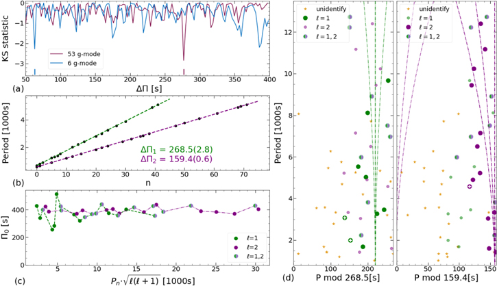
Figure 4. Period spacing and mode identification for independent g-modes. (a) Kolmogorov–Smirnov (KS) tests on two period sets. The vertical segments locate the minimum values for preliminary spacing. (b) The linear fitting for the identified ℓ = 1 and ℓ = 2 modes, respectively, where the slopes indicate the values (text) of their period spacing. (c) The reduced period spacing,  , as a function of the reduced pulsation period. (d) Échelle diagram for dipole (left) and quadrupole (right) modes. The vertical curve locates the corresponding period for rotational components, 3 and 5 for triplet and quintuplet, respectively. The modes marked with white “+” get larger period deviations.
Download figure:
Standard image High-resolution imageBased on the preliminary period spacings, we have identified nine modes as dipole, 13 as quadrupole, and additional eight frequencies which fit both period sequences. We note that the four identified modes include one of the above six dipole modes, f5 ∼ 123.1 μHz. We obtained the average period spacing of 268.5 ± 2.8 s and 159.4 ± 0.6 s for ℓ = 1 and ℓ = 2 modes, respectively, via linear fitting to 17 (4 + 5 + 8) dipole modes and 21 (13 + 8) quadrupole modes (Figure 4(b)). We list ℓ and relative n values in Table 1. We note that the real radial order can only be obtained through seismic modeling. Our results suggest that EPIC 220422705 has a somewhat large period spacing among the known sdB variables, in a range of [220, 270] s for the dipole mode (see, e.g., Reed et al. 2011; Sahoo et al. 2020; Uzundag et al. 2021). As stellar models presented in Uzundag et al. (2021), the evolution tracks suggest that the lower value of period spacing, the lower value of  . This agrees well with a low
  derived for EPIC 220422705. However, atmospheric parameters, with much higher precision, are encouraged for EPIC 220422705 to test the results of Uzundag et al. (2021) in the future.
The échelle diagrams for two sequences are presented in Figure 4(d), where the ℓ = 2 sequence is more consistent than the ℓ = 1 sequence. There are two ℓ = 1 frequencies with larger period deviations, f19 ∼ 324.16 μHz, f30 ∼ 501.25 μHz, whereas only one occurs in the ℓ = 2 sequence, f8 ∼ 218.36 μHz. Asymptotic theory indicates that period spacings are determined by the size of the pulsation resonant cavity (see, e.g., Tassoul 1980) and could be affected by the extent of the convective core (Smeyers & Moya 2007). The ideal pattern for a period sequence in the échelle diagram is a vertical ridge for central components of a star with an internally homogeneous composition. Some deviations from the mean period spacing are to be expected in g-mode pulsating sdB stars—and indeed have already been unambiguously detected in some cases (Østensen et al. 2014)—due to the phenomenon of mode trapping by steep composition gradients. Such deviations reflect properties of the stellar interior, and in particular could reveal the character of the mixing processes at work near the core boundary (see, e.g., Charpinet et al. 2011; Ghasemi et al. 2017). Figure 4(c) shows the deviation of period spacing as a function of the reduced pulsation period. We only observe a large deviation that might be associated with a trapped mode at the fifth order. Indeed, seismic models suggest that strong trapping is more likely found for the lower-order (higher-frequency or shorter-period) modes than the higher-order g modes (Charpinet et al. 2014).
3. Amplitude and Frequency Modulations
This section provides our methodology and characterization of amplitude and frequency modulations (AM/FM) for the most significant frequencies. In practice, we follow the processes as described in Zong et al. (2018) to extract frequency information of subsets of the entire light curve. Here the time interval and window widths are 1 and 30 days, respectively. If close peaks within the frequency resolution (∼0.4 μHz) are detected, we keep the highest peak as the measured value for that frequency. In order to measure AF/FM significantly, frequencies should have amplitudes above 8.8σ of the local noise in each piece of the light curve. This ultimately leads to 22 frequencies that could be analyzed for AMs/FMs, which are marked in the last column of Table 1.
3.1. The Fitting Method
A quick look at all AM/FM patterns occurring in these 22 frequencies suggests that most of them exhibit simple or quasi-regular variations (Figures 5, 6, 7 and 8). In order to quantitatively characterize the modulation patterns, we apply three simple types of fittings: linear, parabolic, and sinusoidal waves. We first calculate standard deviations of our subset data, σ0. Then we adopt a simple AM/RM fitting, typically linear first and then a second type on the residuals. This fitting method may be iterated several times until the residuals present no clear structure and look like random noise. For each fitting, a standard deviation of residuals will be calculated as:

where Gk (t) defines as,
Here k = 1, 2, 3, 4, 5. N denotes the number of data points, and mi is the measured value of amplitude or frequency.
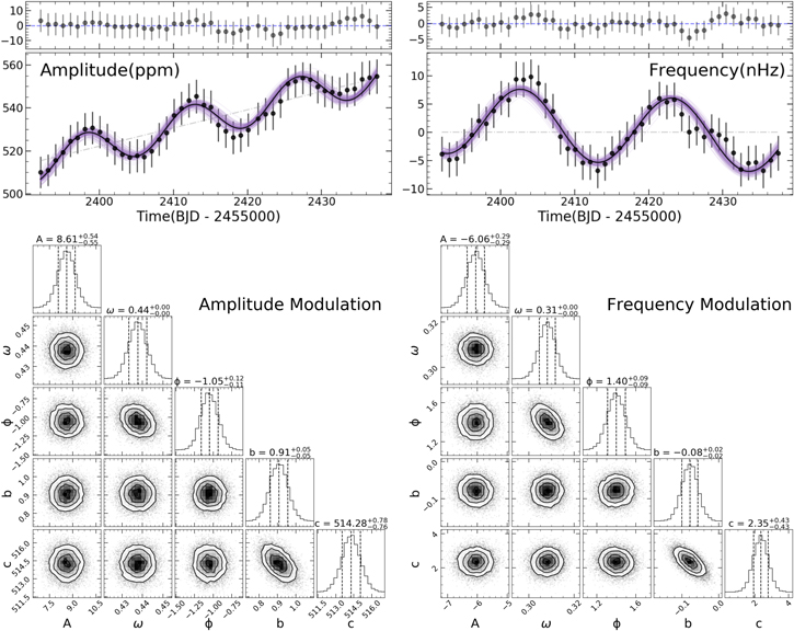
Figure 5. A demonstration of amplitude and frequency modulation for the frequency f3 ∼ 328.75 μHz. The top panels show precise patterns of AM and FM together with the residuals after the best fittings, indicated by solid curves. The shadow curves indicate 100 confidence fitting curves that are randomly taken from Markov Chain Monte Carlo (MCMC) chains. The dashed lines indicate linear relationships to the modulated patterns or constant to zero. The bottom panels show the distributions and the correlations of the five fitting parameters by the MCMC method. The vertical lines, from left to right, define the confidential fittings and stand for 16, 50, and 84 percentiles. The contours are at the 1σ, 2σ, and 3σ levels, respectively.
Download figure:
Standard image High-resolution imageIn principle, the freedom degree of Gk (t) increases as k increases, which in turn results in a lower σk . However, to avoid overfitting of the modulation patterns, for instance, by including a linear or parabolic fitting, we follow the statistical test by Pringle (1975), who defines λ as,

Here Di is the freedom degree of the fitting function, e.g., 2 and 3 for linear and parabola fitting, respectively. A significant improvement for the higher freedom degree fitting should have the parameter that meets the F − distribution, λ > FP=99.75%(D2 − D1, N − D2). For each AM/FM, we prefer to keep the fitting function with a lower freedom degree as indicated by the parameter λ. The results of our fitting for each AM/FM are listed in Table 2, where most frequencies have a sinusoidal component, G3(t), or with an additional linear fitting, G4(t).
Table 2. AM/FM detected in EPIC 220422705, Sorted by Order of Increasing Frequency
| ID | Freq. | Corr. | AM/FM | A | T=2 π/ω | ϕ | a | b | c | Fitting | Comment |
|---|---|---|---|---|---|---|---|---|---|---|---|
| (μHz) | (ppm/nHz) | (d) | [0, 2π) | (10−3) | |||||||
| f7 | 80.5936 | −0.35 | AM |

|

|

| ⋯ |

|

| G4 | I |
| FM |

|

|

| ⋯ | ⋯ | ⋯ | G3 | ||||
| * f5 | 123.0877 | 0.86 | AM |

|

|

| ⋯ |

|

| G4 | B |
| FM |

|

|

| ⋯ |

|

| G4 | ||||
| f16 | 139.9180 | 0.27 | AM |

|

|

| ⋯ |

|

| G4 | I |
| FM |

|

|

|

|

|

| G5 | ||||
| f9 | 143.4188 | −0.37 | AM | ⋯ | ⋯ | ⋯ | ⋯ |

|

| G1 | I |
| FM |

|

|

| ⋯ | ⋯ |

| G3 | ||||
| f12 | 166.8356 | 0.21 | AM | ⋯ | ⋯ | ⋯ |

|

|

| G2 | B |
| FM |

|

|

| ⋯ | ⋯ | ⋯ | G3 | ||||
| f15 | 173.4053 | 0.68 | AM |

|

|

| ⋯ |

|

| G4 | I |
| FM |

|

|

| ⋯ | ⋯ | ⋯ | G3 | ||||
| * f14 | 180.3917 | 0.73 | AM |

|

|

| ⋯ |

|

| G4 | I |
| FM |

|

|

| ⋯ | ⋯ |

| G3 | ||||
| f10 | 187.4747 | 0.14 | AM |

|

|

|

|

|

| G5 | I |
| FM |

|

|

| ⋯ | ⋯ |

| G3 | ||||
| f2 | 207.2400 | −0.15 | AM |

|

|

| ⋯ |

|

| G4 | B |
| FM |

|

|

| ⋯ | ⋯ | ⋯ | G3 | ||||
| f8 | 218.3630 | 0.6 | AM |

|

|

| ⋯ | ⋯ |

| G3 | I |
| FM |

|

|

| ⋯ | ⋯ | ⋯ | G3 | ||||
| f4 | 261.2680 | −0.45 | AM | ⋯ | ⋯ | ⋯ | ⋯ |

|

| G1 | I |
| FM |

|

|

| ⋯ |

|

| G4 | ||||
| f1 | 279.7670 | −0.35 | AM |

|

|

| ⋯ |

|

| G4 | I |
| FM |

|

|

| ⋯ |

|

| G4 | ||||
| * f24 | 288.5611 | −0.88 | AM |

|

|

| ⋯ |

|

| G4 | I |
| FM |

|

|

| ⋯ |

|

| G4 | ||||
| f13 | 299.0409 | 0.67 | AM | ⋯ | ⋯ | ⋯ |

|

|

| G2 | B |
| FM |

|

|

| ⋯ |

|

| G4 | ||||
| f6 | 306.2220 | −0.82 | AM | ⋯ | ⋯ | ⋯ |

|

|

| G2 | I |
| FM | ⋯ | ⋯ | ⋯ |

|

|

| G2 | ||||
| f11 | 311.9932 | 0.12 | AM | ⋯ | ⋯ | ⋯ |

|

|

| G2 | I |
| FM |

|

|

| ⋯ | ⋯ | ⋯ | G3 | ||||
| * f18 | 324.1648 | 0.74 | AM |

|

|

| ⋯ | ⋯ |

| G3 | I |
| FM |

|

|

| ⋯ | ⋯ |

| G3 | ||||
| f3 | 328.7461 | −0.45 | AM |

|

|

| ⋯ |

|

| G4 | I |
| FM |

|

|

| ⋯ |

|

| G4 | ||||
| * f24 | 697.6268 | 0.07 | AM | ⋯ | ⋯ | ⋯ | ⋯ | ⋯ | ⋯ | ⋯ | I |
| FM | ⋯ | ⋯ | ⋯ | ⋯ | ⋯ | ⋯ | ⋯ | ||||
| f17 | 2768.5293 | 0.53 | AM | ⋯ | ⋯ | ⋯ | ⋯ |

|

| G1 | I |
| FM |

|

|

| ⋯ |

|

| G4 | ||||
| f20 | 2781.6577 | 0.19 | AM |

|

|

| ⋯ |

|

| G4 | B |
| FM |

|

|

| ⋯ |

|

| G4 | ||||
| * f44 | 3720.7735 | 0.52 | AM |

|

|

| ⋯ |

|

| G4 | I |
| FM |

|

|

| ⋯ |

|

| G4 |
Note. Columns (1) and (2) The ID and frequency are taken from Table 1. (3) The value of correlation between the amplitude and frequency modulations. (4) The indication of amplitude modulation (AM) or frequency modulation (FM). (5), (6), and (7) The fitting coefficients amplitude (A), period (T = 2π/ω), and phase (ϕ) of sinusoidal function if periodic patterns are found. (8), (9), and (10) The coefficients of polynomial fitting up to second order. (11) The index of fitting function to the modulation pattern. (12) The comments are discussed for the modulation patterns in Section 4.1. B and I denote the beating effect and intrinsic modulations of amplitude and frequency, respectively.
Download table as: ASCIITypeset image
After the fitting function was set, we adopted the posterior distributions based on the Bayesian frame to estimate the best fitting parameters and their uncertainties. The posterior distributions of parameters are sampled by the Markov Chain Monte Carlo (MCMC), which is implemented by the EMCEE code (Foreman-Mackey et al. 2013). The MCMC sampling is performed with more than 22 chains, according to the number of free parameters. It proceeds until the chains converge to values that are inferred by the autocorrelation time module of the EMCEE. Parameters of the best fittings are given by the medians of marginalized posterior distributions, associated with the corresponding errors that are calculated by the half-widths between the 16th and 84th percentiles of the distributions.
Figure 5 is an example of the MCMC application for AM and FM occurring in the frequency f3 ∼ 328.75 μHz. We clearly see that both AM and FM exhibit periodic variations but with different periods and phases. In general, we find that almost all measurements are consistent with the fitting curves, accounting for uncertainties. The best fittings return A = 8.61 ± 0.54 ppm and 6.1 ± 0.3 nHz, T = 14.4 ± 0.1 and 20.4 ± 0.2 days, ϕ = 5.2 ± 0.1 and 1.4 ± 0.1, b = −0.91 ± 0.05 and −0.08 ± 0.02, and c = 514 ± 1 and 2.4 ± 0.4 for AM and FM, respectively.
3.2. Characterization of Modulation Patterns
In this section, we describe the modulation patterns in AM/FM of all 22 significant frequencies except the frequency of f3, which has already been described. Figure 6 is a gallery of 16 frequencies with various modulation patterns, which are identified by different fitting function Gk (t) and summarized in Table 2. In general, the fitting periods of AMs and FMs are on a timescale of months.
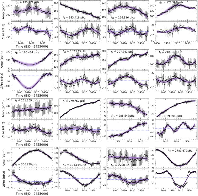
Figure 6. A gallery of 16 frequencies with AM/FM variations. Each module refers to the AM (top panel) and FM (bottom panel) variations of one single frequency. The frequencies are shifted to the average values as represented by the dashed horizontal lines, which are indicated in the bottom panel. The solid curves in purple and black represent the fitting results from the M CMC method and the optimal fitting, respectively.
Download figure:
Standard image High-resolution imageWe now specifically describe these AMs and FMs. A few modes have been observed with simple modulation patterns of only linearly decreasing or increasing in amplitude or frequency. For instance, the amplitude of f9 ∼ 143.4 μHz decreases from 200 to 100 ppm over the time interval of about 50 days. In other observed minor cases, a few modes can be characterized by a simple parabolic fitting, such as the AM/FM of f6 ∼ 306.2 μHz, where both the amplitude and frequency reach their vertex values near the time BJD = 2457420 days. The majority of modulations we observed have quasi-sinusoidal patterns, most with extra linear and a few with parabolic fittings. For example, the amplitude and frequency of f8 ∼ 218.4 μHz exhibit a completely sinusoidal pattern and evolve in phase. Whereas the frequency of f13 ∼ 299.0 μHz demonstrates a sinusoidal pattern with an additional linear fitting. We only find the frequency of f16 ∼ 139.9 μHz and amplitude of f10 ∼ 187.5 μHz show a sinusoidal plus a parabolic pattern. We note that the amplitude of f14 ∼ 180.434 μHz decreases below the detection threshold from BJD − 24554000 = 200 days to 225 days, which holds even if our subsets span 70 d. For most frequencies, a variation of frequency scale is around 20 nHz but there are a few exceptions with large values around 100 nHz. For instance, f20 ∼ 2781.672 μHz, f19 ∼ 324.164 μHz and f23 ∼ 288.547 μHz. The variations of amplitude can span up to a few hundred ppm (f1 ∼ 279.767 μHz) or down to a few ppm (f4 ∼ 261.269 μHz). We note that the amplitudes of AM and FM are not strictly proportional to each other. For instance, the amplitude of f1 increases from about 50 to 250 ppm, but the frequency only varies around 1 nHz.
A very interesting feature of the observed AM/FM is that several frequencies are found with (anti)correlations between AM and FM. We thus calculate the values of correlation for all frequencies as listed in Table 2. The frequencies f23 ∼ 288.561 μHz and f6 ∼ 306.223 μHz all exhibit a strong correlation with a coefficient ∣ρa,f∣ > 0.8 between their amplitude and frequency variation. For instance, f23 and f6 show clear anticorrelation between AM and FM, with derived coefficients of −0.867 and −0.824, respectively. For f23, the amplitude exhibits a slightly decreasing trend, whereas the frequency is the opposite. For f6, its AM and FM are both represented by parabolic fits but with antiphase evolutions. We also note several frequencies with correlated AM and FM patterns showing sinusoidal variations, such as f15 ∼ 173.4 μHz and f8 ∼ 218.3 μHz.
Figure 7 shows another 4 frequencies, f5 ∼ 123.087 μHz, f7 ∼ 80.595 μHz, f11 ∼ 312.0 μHz, and f39 ∼ 3720.7 μHz, whose FM patterns still present modulation structures after fitting by a Gk
(t) function with k = 4, 5. To remove those FM residuals, they needed additional sinusoidal functions, i.e., three fitting functions to present FM patterns. For a strong correlation frequency, f5, with ρa,f = 0.862, exhibits regular AM and FM with periods of  and
and  days, respectively, derived from EMCEE. The other three frequencies, f7, f11, and f39 are determined by EMCEE with either different fitting types of functions or different periods of sinusoidal patterns between AM and FM. For instance, the periods of AM and FM in f7 are calculated as
  and
and  days, respectively, almost with a ratio of 1: 2. The EMCEE returns periods with values of ∼10.3, 19.0, 17.4, and 11.3 days for the additional sinusoidal fittings of the FM residuals of f7, f5, f11, and f39 after extracting Gk
(t), respectively. We note that the FM periods of these residuals are shorter than the periods fitted by Gk
(t).
days, respectively, almost with a ratio of 1: 2. The EMCEE returns periods with values of ∼10.3, 19.0, 17.4, and 11.3 days for the additional sinusoidal fittings of the FM residuals of f7, f5, f11, and f39 after extracting Gk
(t), respectively. We note that the FM periods of these residuals are shorter than the periods fitted by Gk
(t).
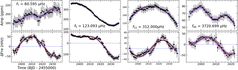
Figure 7. Similar to Figure 6 but for four frequency residuals still showing regular patterns. The dashed (red) curves refer to the final fitting with additional components together with the Gk function.
Download figure:
Standard image High-resolution imageFigure 8 presents the AM and FM of the frequency f24 ∼ 697.62 μHz that shows a quasi-regular behavior but cannot be described by simple fittings of Gk functions, which is also suggested by the fine profile of the LSP and the sliding LSP (sLSP). Thus we do not perform fitting and EMCEE on its AM and FM. We observe that both the AM and FM began with a decreasing trend: the amplitude went down from ∼80 ppm to a local minimum value of ∼60 ppm and the frequency varied from +120 nHz down to −100 nHz relative to its averaged frequency. Then the frequency and amplitude experienced an increasing trend. The amplitude reaches its maximum with a time interval of about 30 days but passes across one stationary point, whereas the frequency generally goes up to around the average value with a back and forth trend.
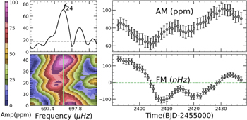
Figure 8. AM and FM of f24 ∼ 697.6 μHz, a frequency that cannot be fitted by the simple function of Gk . The top left panel shows the local LSP where the dashed horizontal line is the 5.2σ threshold. The bottom-left panel provides the sLSP around that frequency and the color bar (indicating amplitude) is shifted to the leftmost side, in which the vertical line is the averaged frequency. Precise measurements of amplitude and frequency variations are presented in the top- and bottom-right panels, respectively. The frequencies are shifted to their average as indicated by the horizontal line.
Download figure:
Standard image High-resolution image4. Discussion
In this section, we will discuss the potential interpretation of the observed AM and FM for all 22 frequencies of EPIC 220422705. Most of those modulations can be fitted with simple functions, Gk (t), with most having sinusoidal fittings. They could be induced by the resonant coupling mechanism that predicts periodic amplitude and frequency modulation as a consequence of nonlinear weak interaction between different coupling modes (see, e.g., Dziembowski 1982; Buchler et al. 1995). However, the relatively short duration of K2 photometry may suffer from other effects on the observed AMs and FMs, such as beating between unresolved frequencies. We therefore generate a series of quantitative simulations of close signals and compare the modulation patterns of those unresolved frequencies with the observed patterns of AM/FM.
4.1. Presence of Closely Spaced Frequencies
As presented in Section 2.3, we detected several potential rotation multiplets with frequency spacings of about 0.2 to 0.4 μHz, which is comparable to the frequency resolution determined by the observation duration, Δf ≈ 1/T. This finding suggests that close frequencies, not only the multiplets we found, may be present in EPIC 220422705 with a very high probability. In literature, many sdBV stars are resolved with such nearby frequencies from the original 4 yr Kepler observations (see, e.g., Zong et al. 2018; Foster et al. 2015; Baran et al. 2012). Those close frequencies will induce amplitude variations, not frequency variations, called beating, if they are unresolved, as demonstrated in Zong et al. (2018). Here we only take two close frequencies as an example,
If we consider two comparable amplitudes, A1 ∼ A2 = A, and a very small frequency separation, Δω ≪ ω0, the Equation (8) will be reduced to
The above equation indicates that two close frequencies will generate amplitude modulations if they are not resolved. We thus have to evaluate this effect on the observed AMs in EPIC 220422705.
A series of simulations was performed to quantitatively compare the observed and calculated AMs. The simulation process is similar to that of Zong et al. (2018), including light-curve construction and frequency injection, but adopted to K2 observations. In practice, we set three parameters A1, A2, and Δω to be constant in the construction of each light curve based on Equation (8) and phase to be zero for simplicity. We then make all parameters as variants in a series of 1331 light curves, with A1, A2 ∈ [0.5, 0.6, ..., 1.5] × A0 and Δω ∈ [0.1, 0.12, 0.14, ...0.3] μHz. Then we transform the simulated light curves into sLSP and directly compare them with the observed sLSP via direct subtraction. Both types of sLSPs have to be transformed into the same time step and window length and scaled to the same maximum amplitude. The flatness of the residual sLSP defines the goodness of similarity between the two sLSPs. We finally select an optimal sLSP for the simulation and return the parameters.
Figure 9 shows the comparison results for five representative frequencies, f9 ∼ 143.4 μHz, f13 ∼ 299.0 μHz, f11 ∼ 312.0 μHz, f24 ∼ 697.6 μHz, and f20 ∼ 2781.6 μHz. We can conclude that the modulations of f13 and f20 are potentially induced by two close frequencies as revealed by no significant residuals. The modulation of f11 and f24 can hardly be simulated by two close frequencies, which indicates the AM and FM to be intrinsic, as revealed by the complex structure of the residual sLSP. The sLSPs of f9 suggest that it is dominated by the beating effect but also experienced intrinsic AM and FM. We list the results of simulations in the last column in Table 2 as “B” for the completely beating effect and “I” for intrinsic modulation. Here we note that the index “I” may also contain beating effects such as the close multiplets discovered, but their AMs cannot be completely represented by those beating effects. In summary, we found that five frequency modulations can be attributed to beating, f5 ∼ 123.1 μHz, f12 ∼ 166.8 μHz, f2 ∼ 207.2 μHz, f13 ∼ 299.0 μHz, and f20 ∼ 2781.1 μHz. Their modulations will not be discussed later. However, the other 17 frequencies are not well represented by beating and must suffer from intrinsic modulations in amplitude and frequency.
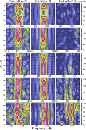
Figure 9. Comparison of sliding LSP of five representative frequencies between observations and simulations. The left, middle and right panels are the observed modulations, the simulated modulations, and the residuals. The flatness of residuals fluctuates gradually worse from top to bottom panels. The residuals present double ridge structures if the sLSP cannot be simulated merely by two close signals.
Download figure:
Standard image High-resolution image4.2. Potential Interpretation of Intrinsic Modulation
As stated above, in EPIC 220422705 many frequencies exhibit intrinsic AM and FM even though they may be contaminated by unresolved frequencies limited by K2 observing duration. These kinds of variations have previously been investigated for several sdBV stars (Zong et al. 2016a, 2018, 2021), showing several characteristics of their modulation patterns: stable, regular, irregular, or complex features. In contrast to Kepler sdBV stars, the observed AMs and FMs here can only be determined for shorter temporal modulations or suffering from the beating of close frequencies. For instance, Zong et al. (2016a) found that in KIC 10139564 the modulating period is about 600 days for the dominant triplet, which is much longer than the derived periods of months in EPIC 220422705.
From a theoretical perspective, we expect various types of AMs and FMs when perturbation theory is extended to nonlinear orders where different resonant modes can have weak interactions governed by amplitude equations (see, e.g., Dziembowski 1982; Buchler & Goupil 1984; Buchler et al. 1995; Moskalik 1985; Buchler et al. 1997). Both in multiplet resonance and direct parent–daughter resonance (e.g., fi + fj ∼ fk ), the frequency mismatch, δ f = fi + fj − fk , is a key parameter to determine the modulating timescale together with the coupling coefficients and linear damping and growth rates. The latter ones cannot be directly obtained from observation, while δ f can be measured if the consecutive subset light curves are long enough. The values of those quantities determine the exact modulation patterns of AMs and FMs.
We do not provide direct calculations of nonlinear amplitude equations constrained by the observed results since many of the physical quantities are not currently available. The linear growth/damping rates and coupling coefficients need sophisticated seismic models before they can be determined. Once those physical quantities are available, we could constrain the growth/damping rates using the observed modulation periods provided in this analysis. At least we can conclude that oscillation modes are unstable, and this characteristic is a ubiquitous phenomenon in oscillation modes of these pulsating sdB stars.
Other mechanisms can also produce frequency modulations but in a systematic trend. For instance, magnetic cycles generally lead all frequencies to shift with a similar pattern (Salabert et al. 2015). The magnetic field is very rare or completely absent in sdB stars (Landstreet et al. 2012), except for one particular object claimed to be produced through the merger channel (Vos et al. 2021). In addition, sdB stars have very stable radiative envelopes and are not known to show magnetic cycles. Frequency or phase modulations can be induced by orbital companions through periodic variations of light traveling time (Silvotti et al. 2007, 2018; Murphy & Shibahashi 2015). This kind of FM for all frequencies has to be found with an identical orbital period and phase. EPIC 220422705's FMs and AMs cannot be well explained by the above two mechanisms in terms of their modulation patterns. Montgomery et al. (2020) recently proposed that temporal changes in depth of a surface convective zone can distort the coherent pulsations in hydrogen atmosphere white dwarfs. That could produce AMs and FMs in sdB stars, but there is no significant convective zone near the surfaces of sdB stars. They also claim a much wider frequency width than what we observed in EPIC 220422705.
5. Conclusion
We have analyzed the nearly consecutive K2 photometry spanning ∼76 days on EPIC 220422705, a g-mode-dominated hybrid pulsating sdB star. A rich frequency spectrum with 66 independent frequencies is detected above the 5.2σ threshold. We attribute 12 frequencies to unresolved rotational multiplets. Rotational periods of  ,
,  , and
, and  days were derived based on six dipole g modes, three quadrupole g modes, and three dipole p modes, respectively. This suggests that EPIC 220422705 has a differential rotation with a slightly slower core than the envelope. The period spacings within the asymptotic regime are derived with ∼268.5 s and 159.4 s for dipole and quadrupole modes on average, respectively. We thus identified nine dipole modes and 13 quadrupole modes with eight additional periods that could fit both sequences.
We characterize 22 significant frequencies with amplitude and frequency modulations. All those frequencies show clear modulation patterns, which are then fitted with simple functions, and their uncertainties were tested by MCMC simulations. Most of those AMs and FMs can be fitted with periodic patterns with periods on a timescale of months which is relatively shorter than that found from Kepler sdBV stars (Zong et al. 2018). A notable feature of the modulations we detect is that they exhibit (anti)correlations between their amplitude and frequency, a similar result to that in Kepler sdBV stars. Limited by the duration of K2 photometry, we have not performed any detailed characterization of the relationship between resonant modes of those modulations, since the frequency resolution is not precise enough.
To quantitatively determine whether the discovered modulations are intrinsic or result from two close frequencies, a series of close frequency simulations were produced and sliding LSPs were compared for each of the 22 frequencies. Only five frequencies are well represented by two close frequencies. Thus we conclude that 17 frequencies have AMs and FMs, which must be intrinsic modulations.
A natural interpretation for such mode variability is the nonlinear mode interactions through resonance (see, e.g., Buchler et al. 1995). Depending on the physical quantities in the amplitude equations, resonant modes can have various types of modulation patterns both in amplitude and frequency. We have expelled other mechanisms account for our findings, although they can also generate AM and FM, for instance, phase variations as depth-of-convective-zone changes (Montgomery et al. 2020). Finally, our results are the first step to precisely characterize the patterns of mode modulations in sdB stars from K2 photometry. Similar to recent results from Kepler (e.g., Zong et al. 2021), as well as several compact pulsators in the continuous view zones of TESS to be analyzed, these AMs and FMs will open a new avenue to develop nonlinear stellar oscillation theory in the near future.
We thank an anonymous referee for their comments to improve the manuscript and the helpful discussion with Dr. Li Gang, Guo Zhao, Zhang Xianfei, and Prof. Wei Xing. We acknowledge the support from the National Natural Science Foundation of China (NSFC) through grants 11833002, 11903005, 12090040, and 12090042. W.Z. is supported by the Fundamental Research Funds for the Central Universities.
S.C. is supported by the Agence Nationale de la Recherche (ANR, France) under grant ANR-17-CE31-0018, funding the INSIDE project, and financial support from the Centre National d’Études Spatiales (CNES, France). The authors gratefully acknowledge the Kepler team and all who have contributed to making this mission possible. Funding for the Kepler mission is provided by NASA's Science Mission Directorate.
Footnotes
- 7
- 8
The EVEREST, as developed by Dr. R. Luger, is an open-source pipeline for removing ∼6.5 hr instrumental systematics in K2 light curves. One can see details through the link: https://archive.stsci.edu/hlsp/everest.
- 9
Frequency Extraction for Light-curve exploitation, developed by S. Charpinet, greatly optimizes the algorithm and accelerates the speed of calculation when performing frequency extraction from dedicated consecutive light curves. See details in Charpinet et al. (2010, 2019) and Zong et al. (2016b, 2016a).