Abstract
While β Pic is known to host silicates in ring-like structures, whether the properties of these silicate dust vary with stellocentric distance remains an open question. We re-analyze the β Pictoris debris disk spectrum from the Spitzer Infrared Spectrograph (IRS) and a new Infrared Telescope Facility Spectrograph and Imager spectrum to investigate trends in Fe/Mg ratio, shape, and crystallinity in grains as a function of wavelength, a proxy for stellocentric distance. By analyzing a re-calibrated and re-extracted spectrum, we identify a new 18 μm forsterite emission feature and recover a 23 μm forsterite emission feature with a substantially larger line-to-continuum ratio than previously reported. We find that these prominent spectral features are primarily produced by small submicron-sized grains, which are continuously generated and replenished from planetesimal collisions in the disk and can elucidate their parent bodies’ composition. We discover three trends about these small grains: as stellocentric distance increases, (1) small silicate grains become more crystalline (less amorphous), (2) they become more irregular in shape, and (3) for crystalline silicate grains, the Fe/Mg ratio decreases. Applying these trends to β Pic’s planetary architecture, we find that the dust population exterior to the orbits of β Pic b and c differs substantially in crystallinity and shape. We also find a tentative 3–5 μm dust excess due to spatially unresolved hot dust emission close to the star. From our findings, we infer that the surfaces of large planetesimals are more Fe-rich and collisionally processed closer to the star but more Fe-poor and primordial farther from the star.
Original content from this work may be used under the terms of the Creative Commons Attribution 4.0 licence. Any further distribution of this work must maintain attribution to the author(s) and the title of the work, journal citation and DOI.
1. Introduction
Debris disks are planetary systems that contain dust, planetesimals, planets, and gas (Hughes et al. 2018), and they provide important insights into planet formation. Theoretical models suggest that two main mechanisms efficiently remove dust grains. Stellar radiation pressure removes grains smaller than the so-called “blowout size” from debris disks (Dent et al. 2014), while it causes the micron-to-millimeter grains to drift toward their star via the Poynting–Robertson (P-R) effect (Guess 1962). However, debris disks are observed to be dust-rich, containing grains with a wide range of sizes from submicron to several millimeters in diameter. The presence of sub-blowout-sized grains in observations points to an active dust replenishing mechanism: collisions among parent bodies such as planetesimals, asteroids, and/or unseen planets. The Spitzer Space Telescope has revealed signatures of such collisional activities in the mid-infrared (MIR) wavelengths through spectroscopy, imaging, and time-series photometry (Chen et al. 2020).
The properties of small dust grains in debris disks, such as crystallinity and Fe-to-Mg abundance, inform us about properties of their larger parent bodies and offer a direct comparison with asteroids and Kuiper Belt Objects (KBOs) in the solar system. In the solar system, asteroidal and cometary relic planetesimals are abundant with crystalline silicates (Lisse et al.2006, 2007; Brownlee 2008; Reach et al. 2010; Wooden et al. 2017). Specifically, comets that originate from the trans-Neptunian region contain Mg-rich silicates (Wooden et al. 2017), whereas asteroids and chondrites originating from the asteroid belt are Fe-rich (Le Guillou et al. 2015). Similar to the solar system, a significant fraction ( ∼ 25%) of debris disks are also found to contain crystalline silicate grains (Chen et al. 2014; Mittal et al. 2015). However, most of these disks are too far to be spatially resolved, and thus we cannot map the crystallinity or Fe-to-Mg ratio in these disks.
As one of the few nearby (20 pc) systems that can be spatially resolved by existing telescopes, β Pic provides us with the opportunity to compare its dust distributions and properties with solar system dust grain distributions and properties. β Pictoris (β Pic) is a 20 Myr old A-type dwarf star and hosts dust, planetesimals, gas, and at least two planets (Lagrange et al. 2009, 2010, 2020; Nowak et al. 2020). Ground-based MIR spectra and images of the β Pic disk have revealed MIR thermal emission attributed to amorphous and crystalline silicate species (Weinberger et al. 2003; Telesco et al. 2005). These silicate species display distinct spatial structures (Okamoto et al. 2004). Specifically, high angular resolution spectroscopy with Subaru COMICS has shown that the crystalline silicates are located toward the center of the disk, and submicron-sized amorphous silicates are distributed in three concentric rings (Okamoto et al. 2004; Wahhaj et al. 2003). However, ground-based MIR observations are inherently limited by the sky thermal background and are unable to resolve regions beyond 30 au from the star, missing the majority of the disk that spans out to 1400 au in the Spitzer Multiband Imaging Photometer (MIPS) 24 μm image (Ballering et al. 2016) and 1800 au in the scattered-light image (Larwood & Kalas 2001).
Space-based mid and far-infrared (FIR) observations enable both the discovery and characterization of cool crystalline silicates in the far out regions of the β Pic disk that are inaccessible to ground-based observations. The Spitzer Infrared Spectrograph (IRS) has detected forsterite emission bands at 28 and 33.5 μm, indicating a cool crystalline silicate population (Chen et al. 2007). The Herschel Space Observatory’s FIR Photodetector Array Camera and Spectrometer (PACS) has revealed a separate population of cool crystalline forsterite through the 69 μm forsterite band. These silicates have been found to have a Mg/Fe ratio of 99: 1 (de Vries et al. 2012). Such a Mg-rich silicate grain composition suggests that the parent bodies, planetesimals, are primitive and unprocessed, similar to the comets seen in the Kuiper Belt in our solar system.
Since the β Pic debris disk contains multiple populations of silicates, our goal is to investigate whether there are any trends in dust properties as a function of wavelength. In this work, we re-extract the β Pic Spitzer IRS spectrum using Advanced Optimal extraction (AdOpt; Lebouteiller et al. 2010) and re-analyze the silicate properties in the spectrum. In addition, we measure the 0.7–3 μm spectrum with the NASA Infrared Telescope Facility (IRTF) Spectrograph and Imager (SpeX) to better constrain the stellar properties. In Section 2, we describe the IRTF observations and the re-reduction of the Spitzer IRS observations. In Section 3, we present our photosphere modeling. In Section 4, we describe our modeling of the photosphere-subtracted thermal continuum and silicate emission features in detail. In Section 5, we analyze the abundance of dust grain species and the trends in grain properties. In Section 6, we discuss the implications of trends in grain properties. We conclude our paper in Section 7.
2. Observations
2.1. SPEX
We observe the β Pic system using NASA’s IRTF Medium Resolution SpeX in its short wavelength cross-dispersed (SXD; R ∼ 2000, 0.7–2.55 μm) and long wavelength cross-dispersed (LXD; R∼2500, 1.7–5.5 μm) modes (Rayner et al. 2003) on 2021 February 2 at 05:47:18 UT and 07:12:12 UT. We use nearby (within 0.5 deg and 0.1 in airmass) HD 37781 (A0V, K = 6.516) as a calibration standard to measure the atmospheric effects on our observations of β Pic. We observe β Pic and HD 37781 in SXD mode with a total on-target integration time of 92 s and 180 s, and in LXD mode for a total on-target integration time of 66 s and 637 s, respectively, at an airmass ∼3. Both stars are observed in ABBA nod mode for telescope and sky background removal.
We reduce our data using Spextool v4.1 (Cushing et al. 2004; Vacca et al. 2003). The calibrated β Pic SXD spectrum has a signal-to-noise ratio (S/N) of 100–300, similar to that of the calibrator HD 37781. However, although the β Pic LXD has an S/N of 100–300, most regions in the calibrator’s LXD have an S/N < 1, due to insufficient on-target integration time (calibrator is ∼4 mags fainter than β Pic). As a result, the calibrated β Pic spectrum has S/N ≥ 10 only at wavelengths 1.7–2.55 and 3.0–4.0 μm. The region in between these windows is heavily impacted by the atmospheric transmission window.
We perform absolute flux calibration of the IRTF SXD spectrum using ESO VLT/NACO JHK photometry (Bonnefoy et al. 2013). First, we calculate the synthetic photometry  ,
,  , and
, and  by convolving the SXD spectrum with NACO JHK’s filter transmission functions. Next, we calculate a scaling factor

We calculate a scaling factor CSXD of 1.04, indicating that the FSXD for JHK bands are on average 4% dimmer than FNACO for JHK bands. This 4% difference is within the IRTF SpeX instrumental accuracy (5%; Rayner et al. 2003). Therefore, we multiply the IRTF SpeX spectrum by 1.04 to be consistent with NACO photometry data. The S/N of the LXD spectrum is limited by the S/N of the standard star and thus suffers from a ∼30% loss in brightness compared to the L’ band photometry. In addition, the LXD spectrum is heavily impacted by the atmospheric transmission. Therefore, we do not perform any further analysis on the LXD spectrum.
2.2. Spitzer IRS
We re-extract and re-calibrate the Spitzer IRS (Houck et al. 2004) low-resolution β Pic spectrum (originally published in Chen et al. 2007) with the most up-to-date IRS extraction and calibration tools (Lebouteiller et al. 2010). In the original β Pic spectrum, Chen et al. (2007) discovered the 23 and 35 μm crystalline silicate emission bands. However, their spectrum displays “sawtooth” fringing patterns as a result of detector artifacts that were not able to be corrected for at the time. With advancements in both Spitzer science center pipelines and knowledge of empirical point-spread functions (PSFs), we now attempt to minimize those detector artifacts that could mask astrophysical signals. In the following subsections, we describe in detail our procedures for re-extracting and re-calibrating the β Pic observations.
IRS is an MIR spectrograph that covers 5.2 − 38 μm with low (R ∼ 60–130) and moderate (R ∼ 600) resolution spectroscopic capabilities, and has two operating modes: a mapping mode and a staring mode. For our work, we focus on low-resolution observations of β Pic. The low-resolution mode consists of two modules, short-low (SL) and long-low (LL). Both have three grating orders with two main orders SL1, SL2, LL1, and LL2 and a short “bonus” order (SL3, LL3). Since SL3 (LL3) is observed simultaneously with the SL1 (LL1) and shares the same observation setups, we omit a separate description of SL3 (LL3). β Pic is observed with a combination of mapping mode and staring mode. See Table 1 for details. All low-resolution observations are made with the spectrographlong slit aligned along the position angle of β Pic disk to within 15°. We describe details in the following subsections.
Table 1. Observation Setup
| Order | Wavelength | Mode | Date | AOR Key | # Pointings | Pointing Extracted | Slit Size | Plate Scale |
|---|---|---|---|---|---|---|---|---|
| (μm) | (”/pix) | |||||||
| SL2 | 5.2–7.7 | Mapping | 2004 Nov 16 | 9872288 | 7 | Exp 4 | 57″ × 3.7″ | 1.8 |
| SL3 | 7.3–8.7 | Mapping | 2004 Nov 16 | 8972544 | 11 | Exp 6 | 57″ × 3.6″ | 1.8 |
| SL1 | 7.4–14.5 | Mapping | 2004 Nov 16 | 9872288 | 11 | Exp 6 | 57″ × 3.6″ | 1.8 |
| LL2 | 13.9–21.3 | Mapping | 2005 Feb 9 | 9016832 | 5 | Exp 3 | 168″ × 10.5″ | 5.1 |
| LL3 | 19.4–21.7 | Staring | 2005 Feb 9 | 9016832 | 2 | Exp 1, 2 | 168″ × 10.7″ | 5.1 |
| LL1 | 19.9–38.0 | Staring | 2004 Feb 4 | 9016064 | 2 | Exp 1, 2 | 168″ × 10.7″ | 5.1 |
Note. “SL” stands for short-low module and “LL” stands for long-low module. See Figure 1 for a visualization of mapping mode dither patterns.
Download table as: ASCIITypeset image
2.2.1. β Pic Observations Using the IRS Mapping Mode
During SL2, SL3, SL1, and LL2 observations, Spitzer mapped the vertical extent of the disk by stepping the telescope across the disk at a specific number of positions (number of pointings in Table 1), each separated by 18 except for LL2 (2
1 for LL2). Because the slits are long and narrow (slit size), the disk is only fully captured in the slit in the central map position (pointing extracted), where the star is well centered in the slit in the dispersion direction. Figure 1 shows a cartoon of three SL2 pointings including the central pointing (exposure 6). In the rest of the pointings, the midplane of the disk is outside of the slit and results in low S/N. Thus, we only perform analysis on the central pointing.
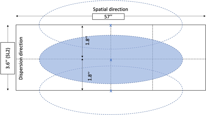
Figure 1. A cartoon illustration of the position of the β Pic disk with respect to the SL slit (57″ × 36 slit) for the IRS SL1 and SL2 mapping mode observations. The telescope was stepped across the β Pic disk in the dispersion direction in increments of 1
8 with the disk well centered in the central pointing as illustrated by the shaded ellipse. The pointings represented by the dotted empty ellipses are not centered in the dispersion direction. The LL2 observations follow similar mapping patterns, where only the central pointing is well centered in the dispersion direction. Drawing not to scale.
Download figure:
Standard image High-resolution imageFor well-centered exposures, we compare slit sizes with the size of β Pic disk and determine the effect of telescope PSF on SL and LL observations to ensure that the disk is completely captured in the slit. Since Spitzer is diffraction-limited, the PSF scales as 1.22 λ/D, where D is the diameter of Spitzer’s mirror and λ is the wavelength. For SL observations, the PSF is 15 (1 pixel) at 5 μm and 4
4 (2.5 pixel) at 15 μm. For LL observations, the PSF is 4
4 (0.9 pixel) at 15 μm and 10
4 (2 pixel) at 35 μm. We find that the β Pic disk roughly spans 3 pixels (approximately 15″) 15 μm in the radial direction and therefore the slits are long enough to capture the entire disk. We also find that disk is spatially resolved in both SL and LL and plan to publish the spatially resolved IRS spectra of the β Pic disk in a subsequent paper. We measure the misalignment angle between the LL slit position angle (PAslit = 44.97 ± 0
02) and disk midplane PA (PAdisk = 29
51) to be 15°. We overlay the IRS LL2 slit on top of the data for a visualization (see
We re-extract SL1,2,3 and LL2 spectra with AdOpt (Lebouteiller et al. 2010). AdOpt first uses empirical super-sampled PSFs to simultaneously fit the PSF to all of the pixels in the spatial direction of the slit and determine weights for individual pixels. In doing so, AdOpt weights the pixels in the extraction window by their S/N and position on the detector to measure the flux at every wavelength. We do not observe any obvious effects of fringing in the extracted SL1,2,3, and LL2 spectra and therefore do not apply fringing correction.
2.2.2. β Pic Observations Using the IRS Staring Mode
The β Pic LL1 and LL3 spectra were observed with IRS staring mode, which stepped the disk at two nod positions (equivalent to pointings) at one-third (Nod 1) and two-thirds (Nod 2) along the slit. First, we extract the spectrum from each nod position with AdOpt. β Pic is well centered in the dispersion direction of the slit in Nod 1 but not well centered in Nod 2. The flux in Nod 2 is 20% lower across all wavelengths than in Nod 1. For the IRS staring mode, the AdOpt supports user-input extraction positions. Therefore, we use the manual optimal extraction option in Spectroscopic Modeling Analysis and Reduction Tool (SMART; Lebouteiller et al. 2010) to adjust the extraction position on the detector plane. We test offset position values between −1 and +1 in 0.1 increments. We find that an extraction offset (offset = −0.39 pixels) best matches the radial profile for the detector image by minimizing the residual (the difference between between the data and extraction profile) across all LL1 wavelengths. After manually extracting the Nod 2 spectrum, we find that the fluxes between Nod 1 and Nod 2 spectra are consistent with one another to within ≤ 1%.
We find artifacts from fringing in LL1 spectra and corrected for them by using an empirical relative spectral response function (RSRF) to correct for out-of-slit light losses. The calibrator star’s RSRF spectrum is defined as the model photosphere divided by the empirical spectrum and therefore characterizes the detector artifacts across pixels. We construct a 1D RSRF for the LL1 wavelength range using a standard K giant star, ξ Dra. ξ Dra was observed on 2005 February 12 (AOR key 13195008) as a part of the IRS calibration program (Sloan et al. 2015). Since ξ Dra is very bright in the mid IR (7 Jy at 15 μm) and has no observed infrared excess, its spectrum is approximately a bare stellar photosphere. We divide out a normalized ξ Dra IRS spectrum from the β Pic spectrum for the RSRF correction. The fringe-correction is effective in removing the fringing effects (e.g., bumps and wiggles) from the spectrum.
2.3. Absolute Flux Calibration and Order Stitching
We perform absolute flux calibration by pining the LL1 spectrum to the MIPS 24 μm flux using LL1 as an anchoring order to calibrate the rest of LL and SL spectra. First, we perform our own MIPS 24 μm aperture photometry extraction by measuring the flux of the unresolved point source in the MIPS 24 μm image. We cannot use existing MIPS 24 μm photometry reported in Ballering et al. (2016) as AdOpt’s extraction window differs from that used by Ballering et al. (2016). AdOpt weights the extraction for the pixels by their S/Ns and their relative positions on the detector. In doing so, AdOpt emphasizes the contribution from the high S/N unresolved point source. Specifically, we calculate the MIPS 24 μm flux, F24 μm,MIPS, that is consistent with an unresolved point source, using aperture photometry with a radius of 3.5″. We use the IDL-based tool, Image Display Paradigm #3 (Lytle et al. 1999) with background subtraction and aperture correction. We choose an annulus with an inner radius of 30″ and an outer radius of 305 from disk center as the background, because the disk attenuates out to roughly 30″ (Ballering et al. 2016). Next, we multiply our extracted flux by 2.57, the aperture correction given in the MIPS Instrument Handbook for a 3.5″ aperture. We estimate F24 μm,IRS, the synthetic photometry from the IRS spectrum. We convolve the MIPS 24 μm filter response function with the IRS spectrum. For the unresolved central point source, we estimate the F24 μm,MIPS = 6.66 Jy and the F24 μm,IRS = 7.01 Jy. Therefore, we apply a scaling factor CIRS = F24 μm,IRS/F24 μm,MIPS = 0.95 to the IRS observations to make them consistent with the MIPS 24 μm observations. We report this scaling factor and any subsequent ones in Column 5 of Table 2 and photometry data in Table 3.
Table 2. Absolute Flux Calibration Parameters
| Order | Wavelength | Ref. Order or Photometry | Overlapping Wavelength | Scaling Factor |
|---|---|---|---|---|
| (μm) | (Corder ) | |||
| LL1 | 19.9–38.0 | MIPS24 | ⋯ | 0.95 |
| LL3 | 19.4–21.7 | LL1 | 19.9–21.7 | 1.12 |
| LL2 | 13.9–21.3 | LL3 | 19.4–21.3 | 1.18 |
| SL1 | 7.4–14.5 | LL2 | 13.9–14.5 | 1.35 |
| SL3 | 7.3–8.7 | SL1 | 7.4–8.7 | 1.0 |
| SL2 | 5.2–7.7 | SL3 | 7.3–7.7 | 1.07 |
Download table as: ASCIITypeset image
Table 3. Photometric Measurements of β Pic
| Filter | Effective Wavelength Midpoint | Magnitude | Flux | Reference |
|---|---|---|---|---|
| λeff for Standard Filters | ||||
| (μm) | (mag) | (Jy) | ||
| U | 0.3518 | 4.13 ± 0.01 | 40.6 ± 0.4 | (a) |
| B | 0.4407 | 4.03 ± 0.01 | 100.9 ± 1.0 | (a) |
| V | 0.5479 | 3.86 ± 0.01 | 108.0 ± 1.1 | (a) |
| R | 0.6864 | 3.74 ± 0.03 | 93.4 ± 2.6 | (b) |
| J | 1.265 | 3.524 ± 0.009 | 62.4 ± 0.75 | (c) |
| H | 1.66 | 3.491 ± 0.009 | 43.2 ± 0.4 | (c) |
| Ks | 2.18 | 3.451 ± 0.009 | 27.8 ± 0.3 | (c) |
| L | 3.77 | 3.454 ± 0.03 | 10.6 ± 0.03 | (d) |
| W1 | 3.35 | 3.484 ± 0.4 | 12.5 ± 4.3 | (e) |
| W3 | 11.6 | 2.597 ± 0.3 | 2.9 ± 0.6 | (e) |
| W4 | 22.1 | 0.014 ± 0.016 | 7.9 ± 0.8 | (f) |
| MIPS24 (Full Disk) | 23.7 | ⋯ | 7.28 ± 0.73 | (g) |
| IRS 24 (Unresolved Point Source ) | 23.7 | ⋯ | 7.01 ± 0.7 | This Work |
| MIPS24 (Unresolved Point Source) | 23.7 | ⋯ | 6.66 ± 0.67 | This Work |
Note. (a). The General Catalogue of Photometric Data (GCPD) Mermilliod et al. (1997) (b). Ducati (2002) (c). Bonnefoy et al. (2013) (d). Bouchet et al. (1991) (e). AllWISE Source Catalog Wright et al. (2010); Mainzer et al. (2011); Cutri et al. (2012). Note: W1 and W2 have 24% pixels saturated and W3 has 8% of pixels saturated. The saturation affects the measurement’s precision as reflected in the inflated error bars. (f). Morales et al. (2012) (g). Su et al. (2006); Ballering et al. (2016). We exclude W2 photometry because for source brighter than magnitude of 5, W2 photometry becomes unreliable.
Download table as: ASCIITypeset image
We use flux-calibrated LL1 spectrum as an anchoring spectrum to scale the rest of LL and SL spectra in descending wavelength order. There is an overlapping wavelength range (Column 2 in Table 2) between every two adjacent orders (Column 3 in Table 2). To calibrate the flux in an order, we take the data points in its overlapping wavelength range with its reference order and calculate an average flux, forder. We repeat this procedure for its reference order and obtain fref.order. Then, we take the ratio of the two to be the scaling factor Corder = fref.order/forder. Specifically, take LL3, for example: LL3 and LL1 overlap between 19.9–21.7 μm. The scaling factor is  . We report the rest of the scaling factors in Table 2. Finally, we check our absolute flux calibration for the entire IRS spectrum with Wide-field Infrared Survey Explorer (WISE) photometry, and we show that our absolute flux calibration is consistent with WISE in Figure 2.
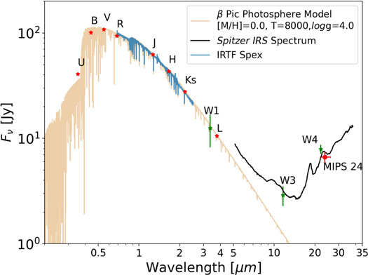
Figure 2.
β Pic SED showing our best-fit model for the stellar photosphere overlaid on UBVRJHKs
photometry (see Table 3) and our 0.7–2.5 μm IRTF spectrum. Our best-fit model has [M/H] = 0.0, Teff = 8000K,  , Av
= 0.078, and RV
= 3.1. The red stars indicate photometry used in the stellar photosphere fitting, and the red circle is the MIPS 24 μm flux derived here for the unresolved central point source. The horizontal error bars indicate the FWHM of the bandwidth for the MIPS 24 μm filter. The L-band photometry indicates that the disk has no infrared excess at 3.77 μm. We omit W2 photometry because it is unreliable for sources brighter than a magnitude of 5.(The data used to create this figure are available.)
, Av
= 0.078, and RV
= 3.1. The red stars indicate photometry used in the stellar photosphere fitting, and the red circle is the MIPS 24 μm flux derived here for the unresolved central point source. The horizontal error bars indicate the FWHM of the bandwidth for the MIPS 24 μm filter. The L-band photometry indicates that the disk has no infrared excess at 3.77 μm. We omit W2 photometry because it is unreliable for sources brighter than a magnitude of 5.(The data used to create this figure are available.)
Download figure:
Standard image High-resolution image2.3.1. IRS Spectrum Uncertainties
We take separate approaches to determine uncertainties for staring mode and mapping mode observations of β Pic. For orders observed in IRS Staring mode (LL1 and LL3), we take the absolute value of the difference in flux between the two nod positions as the uncertainty of the spectra. For orders observed in IRS Mapping mode (SL1, SL2 and LL2 orders), we fit polynomials to part of the spectrum that are not affected by solid-state features. We select regions at 5.6–7.9 and 14.32–14.83 μm of the spectrum and measure the rms of the spectrum from the polynomial fit. We assign the rms as the uncertainty for the spectrum if the rms is bigger than 1% and adopted a 1% error floor according to Higdon et al. (2004). The resulting spectrum is shown in Figure 2.
3. Analysis
In this section, we first describe fitting our new IRTF spectrum and existing photometry with stellar photosphere models to better predict the stellar photospheric emission at MIR wavelengths. We then report our discovery of new silicate emission features from AdOpt extraction. Lastly, we describe our discovery of an infrared excess at 3–5 μm, consistent with the presence of hot dust in the system.
3.1. Stellar Photosphere
We model the β Pic stellar photosphere to understand (1) the relative flux contribution of disk emission to the overall brightness at the shortest wavelength in IRS β Pic spectrum and (2) to rigorously determine the overall shape of the disk emission spectrum. At the H band, Very Large Telescope Interferometer (VLTI) measurements suggest that the β Pic disk emission only constitutes 0.88% of the total emission (Ertel et al. 2014). Similarly, at the shortest wavelengths of the IRS spectrum (5.3 μm), the spectrum is expected to be dominated by the stellar photosphere. We use the VLTI measurement to accurately estimate the brightness of the stellar photosphere at the shortest IRS wavelengths.
To predict the stellar photosphere at 5.5 μm, we fit β Pic’s UBVRJHKs
photometry (Table 3) and IRTF spectrum from 0.7–2.5 μm with BT-NextGen models (Allard et al. 2012; Hauschildt et al. 1999). The addition of an IRTF β Pic spectrum better constrains the model’s spectral slope in the infrared wavelength range. β Pic has an edge-on disk, and therefore the disk might provide a small amount of extinction along the line of sight. Therefore, we assume that extinction, E(B-V), is a free parameter and redden photosphere models using the general extinction law with Rv
= 3.1 with “dust extinction” software. We also include the effect of stellar rotation and limb darkening by convolving photosphere models with a line spread function consistent with  (Claret 2000) and applying a limb-darkening coefficient of 0.24 consistent with the H-band measurements of β Pic (Claret et al. 1995). Our best-fit model has Teff = 8000K, Rv
= 3.1, Av
= 0.078,
(Claret 2000) and applying a limb-darkening coefficient of 0.24 consistent with the H-band measurements of β Pic (Claret et al. 1995). Our best-fit model has Teff = 8000K, Rv
= 3.1, Av
= 0.078,  , and [M/H] = 0.0 with a reduced χ2 = 0.012. Our best-fit values for
  , metallicity, and the Teff are consistent with those reported in the literature (e.g., Pecaut & Mamajek 2013). We note that this fit incorporates extinction as a free parameter for the first time. In Figure 2, we show the β Pic stellar photosphere model, the IRTF spectrum, and the Spitzer IRS spectrum together.
Next, we subtract off our best-fit stellar photospheric model from the IRS AdOpt spectrum. In Figure 3, we plot the photosphere-subtracted AdOpt spectrum of the unresolved point source in blue and the Chen et al. (2007) full-slit extraction spectrum in black for comparison. We can see the change in extraction window sizes brings out a new spectral feature at 18.5 μm and recovers the 23.7 μm crystalline forsterite feature previous reported in Chen et al. (2007) with a higher line-to-continuum ratio.
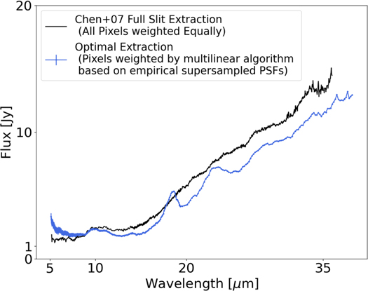
Figure 3. The β Pic IRS spectrum showcasing the newly discovered 18 μm feature and a 23 μm feature with larger line-to-continuum ratio than previously reported by Chen et al. (2007). The optimal extraction (this work) is in blue, while the full-slit extraction published in Chen et al. (2007) is in black. The uncertainties for the spectrum extracted with AdOpt are on average at the 1% level. The Chen+07 spectrum reduced using a full-slit extraction has fringes.
Download figure:
Standard image High-resolution image3.2. Discovery of the New Spectral Features
We discover an 18.5 μm spectral feature. We attribute the discovery of a new 18.5 μm feature to advancements in the knowledge of empirical Spitzer PSFs (Sloan et al. 2015; Lebouteiller et al. 2010). These improvements enable us to (1) extract a spectrum with high S/N in the slit and (2) correct for fringing in the spectrum to further validate the fidelity of the new spectral feature using all of the calibration data obtained during the cryogenic mission. Specifically, compared to Chen et al.’s (2007) full-slit extraction, which weights every pixel in the entire slit equally, our AdOpt spectrum emphasizes the region close to the star. As the S/N increases toward the central star, most of the data points in our spectrum have less than 1% uncertainties.
We conclude that the 18 μm feature must be astrophysical and is emitted by dust grains in the disk. For the newly discovered 18 μm feature, we verify that it is not a detector artifact by examining the entire IRS calibrator star library for LL2 observations to understand detector characteristics. Most fringing patterns only span two to a few (usually five) data points, but our 18 μm feature has an FWHM of ∼ 2 μm that spans more than 30 data points. More importantly, we do not see any 18 μm artifacts in the calibrator star spectra that resemble our new 18 μm feature. Therefore, we rule out the possibility that the 18 μm arises from detector artifacts.
3.3. Constraints on the Spatial Distribution of the New 18 μm Feature
Next, to constrain the spatial distribution of dust grains that are responsible for the 18 μm and 23 μm spectral features, we analyze the Gemini Thermal-Region Camera Spectrograph (T-ReCS) spatially resolved broadband MIR images of the β Pic disk (Telesco et al. 2005). Telesco et al. (2005) took images of the β Pic disk in Qa (central wavelength at 18.3 μm) and Qb (central wavelength at 24.6 μm) bands. In these broadband MIR images, both the disk continuum emission and the characteristic solid-state emission from dust contribute to the flux. As Qa and Qb bandpass’s wavelength range (17.57–19.08 and 23.62–25.54 μm) overlaps with our IRS solid-state emission features (18.5 μm and 23.8 μm), these MIR images can constrain the spatial distributions of the dust grains responsible for the solid-state features. The T-ReCS images are diffraction-limited with beam sizes of 0.356″ (7 au) at 18.3 μm and 0.445″ (9 au) at 24.6 μm, respectively, much finer than that of the Spitzer IRS. Therefore to include the effect of the changing PSF size with wavelength, we convolve the 18.3 μm image with the a PSF profile at 24.6 μm, such that when we take the ratio of two images in subsequent analysis, the PSF will not bias the results.
We find that the majority of the emission at 18.3 μm comes from a region within 2″ (∼50 au) and that 18 μm emission arises from a spatial extent closer to the star than that of the 24 μm emission. As shown in Figure 4, we construct a 1D surface brightness profile of the disk at 18.3 and 24.6 μm. To do so, we exclude the top and bottom 10 rows of pixels to eliminate the background and then sum the flux along the y-axis direction. We find that the 18.3 μm brightness profiles drop sharply at ∼2″, indicating that the majority of the flux at 18.3 μm comes from regions within ∼50 au. We compare the spatial distribution of 18.3 μm emission with that of 24.8 μm by taking the ratio of the two profiles. We find that the F18 μm/ F24 μm flux ratio also drops sharply at ∼ 2″, indicating that the 18.3 μm emission is mostly concentrated in the inner ∼50 au, while the 24.6 μm emission is more spread out throughout the disk. The brightness profiles shown in Figure 16 of Ballering et al. (2016) display a similar conclusion.
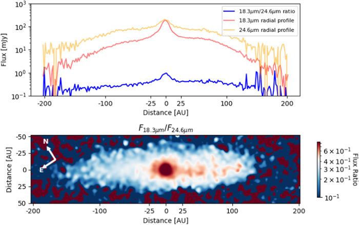
Figure 4. Top: radial surface brightness profile of the 18.3 μm band and 24.6 μm β Pic images from T-ReCS Telesco et al. (2005) imaging and ratio of the surface brightness profile. Bottom: flux ratio between the 18.3 μm band and 24.6 μm from T-ReCS imaging (Telesco et al. 2005). The red color indicates regions in which the 18.3 μm emission is relatively bright compared with the 24.6 μm emission. The bottom panel shows that the 18 micron flux originates from regions (red colors) close to central star (within 10”) while the 24 μm flux originates from more distant regions in the disk (blue).
Download figure:
Standard image High-resolution imageWe estimate the physical location of the grains responsible for the new ∼18 μm emission feature and compare this distance with the semimajor axis (∼10 au) of β Pic b. We assume that the dust is optically thin and is in radiative equilibrium. If the dust grains are large, then they will absorb and emit radiation like blackbodies and be located at the blackbody distance. For example, large dust grains at a distance of 9 au are expected to have a temperature of 160 K and to emit blackbody radiation whose emission peaks at ∼18 μm. However, scattered-light images of debris disks indicate that the blackbody distance tends to underestimate the actual distance of dust by a factor of ∼2 (Schneider et al. 2018). Therefore, the grains that are responsible for the ∼18 μm feature are expected to be located at ∼20 au. For comparison, the β Pic b planet is located at 10 au from the star, interior to the dust that produces the feature 18 μm. Given the loose constraints set by the blackbody distance and the Gemini T-ReCS observations, there is still some uncertainty in the relation of the 18 μm dust distance to the β Pic b planet.
We exclude the possibility that the new 18 μm feature arises from a halo component. Recent modeling of multiwavelength β Pic debris disk images (e.g., Ballering et al. 2016) requires the presence of a spatially extended halo (45–1800 au or ∼ 225 to 90″) of fine dust grains to reproduce the thermal emission spectral energy distribution (SED). If the 18 μm feature were generated in the halo, then the spectral feature would have been present in the full-slit extraction of the beta Pic spectrum (Chen et al. 2007). However, the full-slit extraction does not show an 18 μm micron feature. Our optimal extraction, on the other hand, weights pixel fluxes by their S/Ns in the extraction. In doing so, the extraction heavily weights the emission from the unresolved point source. Specifically, an unresolved point source is expected to have an FWHM of ∼1.5″ at 5 μm and ∼ 7″ at 24 μm (∼ 5″ at 18 μm). Indeed, at 5–7.6 μm, the AdOpt extraction window is too small to include the halo; therefore, we rule out the halo contribution to the spectrum at these wavelengths. At longer wavelengths, the extraction window includes increasingly more of the halo until it reaches a maximum FWHM ∼ 12″ at 40 μm. Even at this longest wavelength, the extraction aperture is not large enough to capture all of the halo flux given the halo geometry from Ballering et al. (2016). Since the full-slit extraction did not reveal the new 18 μm feature, we conclude that the new 18 μm feature in our optimal extraction spectrum is not due to the halo component in the β Pic disk.
3.4. Tentative Evidence of Weak Infrared Excess around 3–5 μm
In the 5–7 μm region, the IRS spectrum is above the stellar photosphere model, indicating a possible excess at 5 μm. The elevated flux in the spectrum is unlikely to be an artifact because the uncertainty in the point-to-point calibration of IRS spectra is less than 1%. This 5 μm excess is tentative evidence for the existence of a hot dust population at ∼ 600 K, which must be physically located within 0.7 au to the star. A 5 μm excess has not been previously reported; however, near-infrared (NIR) interferometric observations have discovered an 0.88% excess at the H band (Defrére et al. 2012; Ertel et al. 2014). We used all of the available photometric measurements including WISE W1, W3, W4, and an L-band measurement from Bouchet et al. (1991) along with our new IRTF SpeX spectra to determine the onset of the NIR excess. As shown in Figure 2, we find that the L-band flux is in good agreement with β Pic’s photosphere model prediction. The lack of infrared excess at 3.77 μm and the infrared excess at 5 μm indicates that there could be a sudden turn-on of infrared excess in that region. This tentative, weak infrared excess indicates that there might be a population of host dust emitting in the wavelength range of 4–5 μm. We discuss the implication of this result in Section 6.3.
We find that the 3–5 μm excess is probably due to thermal emission from hot dust. To first order, light that is scattered off of dust grains has the same SED as the stellar host star. Our discovered 3–5 μm excess does not have a color consistent with a Rayleigh–Jeans blackbody as would be expected for the SED of an A-type star at 3–5 μm. Second, the magnitude of scattered light from the disk is significantly smaller than the observed infrared excess. Even in the brightest cases (Space Telescope Imaging Spectrograph scattered-light images of debris disks), only ∼0.1% of the incident starlight is scattered by the dust (e.g., Schneider et al. 2014). At 5 μm, the IRS AdOpt spectrum has a 30%–50% excess flux with respect to the flux predicted from its stellar photosphere model. Therefore, we exclude the scattered-light hypothesis.
4. Spectral Feature Fitting
In this section, our objective is to find the best-fit models of grain properties—composition, size, shape, and temperature—for the β Pic AdOpt spectrum. To obtain these properties, we first construct a disk model. Next, we select a suite of lab-measured dust optical constants and use them to calculate dust emissivities by varying grain properties. We then describe our fitting procedure. Finally, we report our best-fit models and immediate findings from these models.
4.1. Modeling Disk Continuum Emission
To isolate the solid-state emission from the disk continuum emission, we first model the disk continuum emission by fitting two blackbody components to it. As large grains (10–100 μm) mainly contribute to disk continuum emission, most disk continua can be modeled by a two blackbody model (Mittal et al. 2015). We use 5.61–7.94, 13.02–13.50, 14.32–14.83, 30.16–32.19, and 35.07–35.92 μm regions as anchoring points to fit for two blackbodies. We find the disk continuum consists of a warm blackbody at ∼374 ± 80 K and a cool blackbody at ∼90 ± 10 K by minimizing the χ2 value. We plot the two blackbodies alongside the disk spectrum in Figure 5. The ∼300 K and ∼100 K blackbodies are later used for estimating the temperatures of the small grains, which are responsible for the solid-state emission features. Finally, to obtain a spectrum with only solid-state emission features, we subtract the two fitted blackbodies from the IRS photosphere-subtracted β Pic disk spectrum. In the following sections, we work with this version of the spectrum.
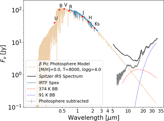
Figure 5. β Pic SED with best-fit blackbodies overlaid. The cool dust component has a temperature of 91 K (blue dotted line) while the warm dust component has a temperature of 374 K (red dotted line). We use these blackbody temperatures to select the temperature-dependent forsterite and enstatite optical constants used in our spectral feature fitting.
Download figure:
Standard image High-resolution image4.2. Modeling Solid-state Emission Features
We investigate the mass and composition of the silicate grains in the β Pic debris disk by fitting the solid-state features in the IRS spectrum. We model the emission from small grains assuming the Rayleigh limit, in which the grain sizes are much smaller than the wavelength of the incident light ( ). Such small grains are responsible for sharp, well-defined spectral features, while the large grains (in β Pic’s case, 10 μm or larger) can only produce very flat spectral features (e.g., Kessler-Silacci et al. 2006; see their Figures 6, 7, 8). Specifically, for β Pic, past analyses have revealed that submicron- sub-blowout-sized grains are abundant in the β Pic disk, indicating an active dust replenishing mechanism (e.g., Okamoto et al. 2004; Czechowski & Mann 2007; Dent et al. 2014; Kral et al. 2016). In addition, as these submicron-sized grains are expected to be the most abundant grain sizes in β Pic, they dominate the emission cross sections according to the power-law number distribution (e.g., f(a) ∝ a−3.5; Dohnanyi 1969; Pan & Schlichting 2012).
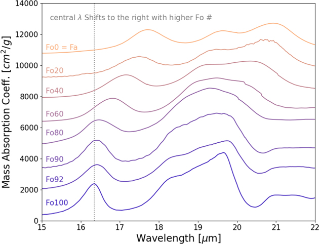
Figure 6. Spectra of forsterite as a function of Fo number at room temperature (∼300 K). The silicate emission feature central wavelengths shift toward longer wavelengths with increasing Fe abundance from the bottom (Fo100 means 100% Mg and no Fe) to the top (Fa means 100% Fe and no Mg). To help visualize the differences among samples, we vertically offset the spectra, adding multiples of 1000 cm2 g−1 to each spectrum. We note that the emission features vary with both the Fo number and silicate temperature. We fix the temperature at ∼ 300 K to showcase the effect of Fo number in this plot.
Download figure:
Standard image High-resolution imageTo describe the size distribution of these submicron-sized grains, we use three shape distributions: spheres (Mie theory), a continuous distribution of ellipsoids characterized by equal probability of all shapes (CDE1 hereafter) and by a quadratic weighting in which extreme shapes such as plates and needles have been removed (CDE2; for the analytical functions of CDE1 and CDE2, see Fabian et al. 2001). The ellipsoids in the CDE distributions can range from prolate ellipsoids such as needles and footballs to oblate ellipsoids such as pancakes and plates. The CDE approximations not only offer analytical solutions for the mass absorption coefficients (MACs), but can also be computed fast enough to quickly explore a large parameter space for different dust compositions at different temperatures and abundances.
We assume that the β Pic debris disk is optically thin at all Spitzer IRS wavelengths, and therefore the exact solution to the disk model is simply the sum of the emission from each grain population. Previous models have shown that the β Pic system is well-approximated using two thin dust rings, each with distinct composition and temperature (e.g., Li & Greenberg1998; Chen et al. 2007). We follow this convention and assume separate temperatures and compositions for each of the two populations. Our model of the disk is similar to that used by Sargent et al. (2009a) to model protoplanetary disks,

where Fν is the flux at each wavelength, Bν is the spectral radiance of a blackbody as a function of temperature, Tc and Tw are the temperatures of the cool and warm components of the disk, respectively, and ac,i (aw,j ) are the mass fraction in which ac,i = mc,i /d2 (aw,j = mw,j /d2). mc,i is the mass of the ith (jth) dust grain species at Tc (Tw ), and d is the distance to β Pic. ac,0 and aw,0 are offset values that account for the disk continuum emission from large grains. κν,i and κν,j are the MAC in cm2 g−1 (or emissivity for simplicity). We note that κν,i for the crystalline silicate species are temperature dependent, but we omit this temperature dependence in the notation.
Our model has a total of 16 free parameters: Tc and Tw , the mass fractions for six species of dust grains with temperatures Tc and Tw , respectively, and two offset values ac,0 and aw,0. Table 4 lists the parameters. We model our spectrum by adapting code developed by Sargent et al. (2009a). Since the Sargent et al. (2009a) study, the library of silicate optical constants has grown, expanding to include measurements with a larger number of Fe/Mg ratios and temperatures (e.g., Zeidler et al. 2015). We tailor the set of optical constants to better fit the β Pic debris disk, leveraging the new laboratory measurements. We require the mass fractions to be nonnegative numbers in the fitting procedure and use χ2 optimization. If the grains were blackbodies with the same emissivity, then the two populations would form two concentric thin rings, each with negligible radial width. However, since our model includes six different species of dust, where each species has distinct emissivities, grains with different compositions but the same temperature will not be colocated. The model can be simply understood as a disk with 12 dust rings, with six rings emitting at Tc and the other six emitting at Tw . Note that our choice of emissivities, κ, is limited to lab-measured optical constants at 100 K, but in reality, the cool grains can vary from ∼ 80 K to ∼ 120 K, and their emissivities will change with temperature.
Table 4. Dust Masses for the Best-fit Models of the β Pic Debris Disk
| Species | Shape | 10 μm | 18 μm | 23 μm | 28 and 33 μm |
|---|---|---|---|---|---|
| (10−3 Mmoon) | (10−3 Mmoon) | (10−3 Mmoon) | (10−3 Mmoon) | ||
| Cool Dust Continuum Temperature (Tc ) | 91 K | 84 K | 82 K | 82 K | |
| Pyroxene (Mg0.7Fe0.3SiO3) | CDE2, Rayleigh Limit | 11.6 ± 2.0 | 0 ± 2.8 | 0 ± 3.6 | 0 ± 3.5 |
| Pyroxene | Mie, 5 μm radius, 60% porosity | 0 ± 1.5 | 0 ± 2.2 | 0 ± 2.7 | 0 ± 2.7 |
| Olivine (MgFeSiO4) | CDE2, Rayleigh Limit | 10.9 ± 1.5 | 34.5 ± 2.3 | 26.0 ± 2.7 | 19.6 ± 2.6 |
| Olivine | Mie, 5 μm radius, 60% porosity | 0 ± 1.0. | 0 ± 1.4. | 0 ± 1.8 | 0 ± 1.7 |
| Forsterite (Mg1.72Fe0.21SiO4) | (1) | 3.5 ± 0.8 | 2514 ± 507 | 4483 ± 594 | 3031 ± 425 |
| Enstatite (Mg0.92Fe0.09SiO3) | (1) | 0 ± 0.7 | 183 ± 564 | 260 ± 250 | 391 ± 474 |
| Warm Dust Continuum Temperature (Tw ) | 374 K | 298 K | 282 K | 272 K | |
| Pyroxene (Mg0.7Fe0.3SiO3) | CDE2, Rayleigh Limit | 0.019 ± 0.003 | 0.046 ± 0.006 | 0.064 ± 0.007 | 0.067 ± 0.008 |
| Pyroxene | Mie, 5 μm radius, 60% porosity | 0 ± 0.003 | 0.017 ± 0.006 | 0.031 ± 0.008 | 0.074 ± 0.009 |
| Olivine (MgFeSiO4) | CDE2, Rayleigh Limit | 0 ± 0.002 | 0 ± 0.004 | 0 ± 0.005 | 0 ± 0.005 |
| Olivine | Mie, 5 μm radius, 60% porosity | 0 ± 0.003 | 0 ± 0.005 | 0 ± 0.006 | 0 ± 0.007 |
| Forsterite (Mg1.72Fe0.21SiO4) | (1) | 0.0024 ± 0.0017 | 0.82 ± 0.81 | 0.82 ± 1.33 | 0.37 ± 1.46 |
| Enstatite (Mg 0.92 Fe 0.09SiO3) | (1) | 0 ± 0.0016 | 0 ± 0.8 | 2.3 ± 1.6 | 1.94 ± 1.69 |
| χ2 | ⋯ | 23.8 | 23.6 | 25.3 | 30.3 |
Note. 1. The shape distribution for forsterite and enstatite are CDE1 for 10 μm feature, Mie for 18 μm feature, CDE2 for 23 μm, CDE1 for 28 and 33 μm features. 2. The warm dust species share the same stoichiometry as the cold dust species. 3. The optical constants for the forsterite and enstatite used for the cool dust are measured at 100 K, while those for the warm dust are measured at 300 K. Therefore, their mass fraction coefficients are independent from each other. 4. The χ2 values calculated for the best-fit models use the full wavelength range (5–35 μm) in the IRS spectrum.
Download table as: ASCIITypeset image
4.3. Dust Emissivity
Past analyses based on spectra and imaging data indicate that grains are predominantly composed of silicates and organics (e.g., Chen et al. 2007; Ballering et al. 2016). Since the IRS β Pic spectrum shows prominent emission features associated with silicates, we investigate lab-measured optical constants for silicate species. The grain composition primarily affects the central wavelength location of emission features. In addition, for every grain species, four additional grain properties (crystallinity, Fe/Mg ratio, shape, and temperature) can shift the central wavelength features around. Therefore, we explore the Jena database for the most suitable optical constant measurements.
First, we select grain species based on the observed central peak wavelengths and rule out the species from visual examinations. We select olivine and pyroxene, which have characteristic features in the 10, 18–20, 23–25, and 28–33 μm regions. We exclude quartz (SiO2), as quartz has sharp and triangular 9 μm features that are inconsistent with our trapezoidal 10 μm feature. We also exclude carbonates because our IRS spectra do not have any 6 μm features that resemble their characteristic features.
Next, we divide the olivine and pyroxene into amorphous and crystalline groups. We use amorphous pyroxene (Mg0.7Fe0.3SiO3) and crystalline pyroxene, which is known as enstatite (Chihara et al. 2002). We also use amorphous olivine (MgFeSiO4) from Dorschner et al. (1995) and crystalline olivine, which is known as forsterite from Zeidler et al. (2015) and Fabian et al. (2001). 12 Since amorphous grains have only two broad emission features (at 10 and 20 μm), their emission features are primarily affected by their size distribution. Therefore, we calculate the emissivities of the small amorphous grains using CDE2 and the emissivities of the large amorphous grains using Mie theory and grains with a 5 μm radius.
For crystalline silicates, there are three grain properties that can shift the peak wavelengths of crystalline grain emission features to a shorter wavelength: (1) a decrease in Fe/Mg ratio, (2) a decrease in the grain temperature, and (3) an increase in the grain sizes or porosity. For (1), the peak wavelengths of the emission features shift toward shorter wavelengths as the Fe/Mg ratio decreases, and toward longer wavelengths as the ratio increases. We show an example in Figure 6 that an 8% increase in the Fe content (from Fo100 to Fo92) broadens and redshifts the bands by 0.18 μm in the 18–20 μm features (Chihara et al. 2002; Koike et al. 2003). 13 For (2), the peak wavelength of the emission feature shifts toward a longer wavelength as the temperature of the crystalline silicate increases. For example, a 200 K decrease in forsterite grain temperature (from 300 K to 100 K) would redshift the peak wavelength by 0.09 μm from 18.95 to 18.85 μm (Zeidler et al. 2015). According to our dust continuum model in Section 4.1, we use the 300 and 100 K lab-measured forsterite and enstatite optical constants. Given that Zeidler et al. (2015) measured the optical constants of forsterite and enstatite on a sparse temperature grid of 10, 100, 200, 300, 551, 738, and 928 K, we choose not to interpolate the grid to obtain finer temperature resolutions to avoid introducing artifacts. Even though our best-fit grain temperature might deviate from these exact values by as much as ∼ 80 K, we only use the optical constants reported in Zeidler et al. (2015). For (3), as the grain sizes increase or become more porous, the spectral features become flatter for both amorphous and crystalline silicates, and the peak wavelength of the feature shifts toward longer wavelengths (Kessler-Silacci et al. 2006). To account for the change in grain emission feature due to size and shape effect, we create three different shape groups for the same species (see Table 4 Column 2) as aforementioned in Section 4.2.
For forsterite, we experiment with the optical constants measured from the San Carlos low-Fe olivine (98.9% Mg-content) sample (Zeidler et al. 2015) at temperatures from 10 K to 928 K. We also experiment with the earlier optical constants from Fabian et al. (2001) measured at room temperature. Among all temperatures, we find that the 100 K, 98.9% Mg-rich forsterite (Fo99) provides the best wavelength match to the IRS spectrum’s 18.5 μm feature. Interestingly, this Fe/Mg ratio is also consistent with the Fe/Mg ratio (99% Mg) measured from the Herschel/PACS 69 μm forsterite band (de Vries et al. 2012), which is highly sensitive to the Fe/Mg ratio (Koike et al. 2003). We also include a 300 K Fo90 component for our warm dust component. In addition, we examine the high-Fe content crystalline olivine (known as fayalite) and find that fayalite has double emission peaks in the range of 15–20 μm. We exclude fayalite from our model, because its spectral features are not consistent with our observed single peak emission feature in the same wavelength range.
For enstatite, we use temperature-dependent optical constants from Zeidler et al. (2015). Similarly, we find that a 98.9% Mg-content enstatite (En99; Zeidler et al. 2015) at 300 K and 100 K has spectral features that are consistent with our IRS emission features. Therefore, we also include them in our suite of emissivities. We also find that past works (e.g., Sargent et al. 2009a, 2009b) demonstrated that the 95% Mg-content forsterite (Fo95; Fabian et al. 2001) and 90% Mg-content enstatite (En90; Chihara et al. 2002) produce good matches with IRS spectra. Therefore, we include an additional set of opacities (Fo95 and En90) as alternative opacities for (Fo99 and En99).
4.4. Fitting Procedures
Based on our blackbody continuum fit described above, we constrain Tc
and Tw
to be within (80, 160) and (260, 380) K. Each temperature range is divided into 11 steps, and hence the uncertainties for the fit are  K and
K and  K. We minimize χ2 for our fit by iterating over these two temperature ranges. For a more in-depth description of the fitting procedure, we refer the reader to Section 3.4 in Sargent et al. (2009b) and Section 3.7 in Sargent et al. (2009a).
4.5. Best-fit Models
We find that β Pic at minimum contains a warm (∼300 K) and a cool (∼100 K) population of dust, where the cool population is mainly responsible for the 18–33 μm emission. We plot our best-fit models in Figures 7, 8, 9, and 10 and tabulate their various species of dust masses in Table 4. The best-fit model shows that the 18 μm feature is mostly emitted by the 100 K cool forsterite. The best-fit model contains 3000 times more cool forsterite mass than the 300 K warm forsterite mass.
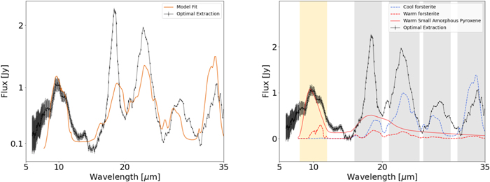
Figure 7. Best-fit model for the 10 μm region. Left: model fit (orange) plotted over the data (black). Right: components of different grain species plotted over the data. Warm and cool dust species are plotted in red and blue, respectively. Flux from all dust species sums to the model fit (orange) in the left panel. We use gray bands to mark the 18, 23, 28, and 33 μm bands where the model does not fit the data well and use pale yellow bands to highlight the areas where the model fits the data well.
Download figure:
Standard image High-resolution imageEven though the 18 μm feature is well modeled in Figure 8, the 23, 28, and 33 μm features are not well modeled. The model-predicted features all have peak wavelengths shorter than the observed peak wavelengths. In Figure 8, gray bands mark the 23, 28, and 33 μm bands where the model does not fit the data well, and pale yellow bands showcase where the model performs well.
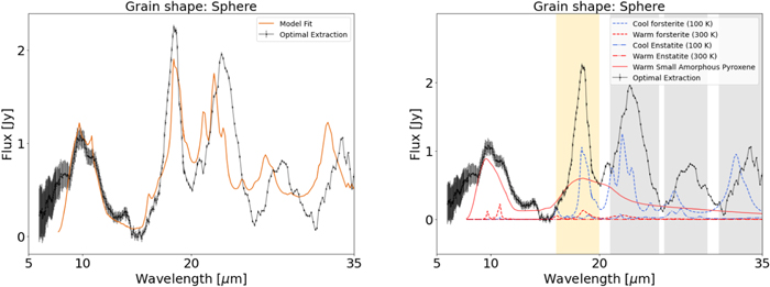
Figure 8. Best-fit model with particle shape calculated with the Mie theory. We show the disk spectrum with its featureless blackbody components subtracted from the total flux. Left: model fit (orange) plotted over the data (black). Right: components of different grain species plotted over the data. Warm and cool dust species are plotted in red and blue, respectively. Flux from all dust species sums to the model fit (orange) in the left panel. We use gray bands to mark the 23, 28, and 33 μm bands where the model misfits and use pale yellow bands to showcase where the model performs well.
Download figure:
Standard image High-resolution imageBy modifying our grain shapes to be a moderate continuous distribution of ellipsoids (CDE2), we optimize the fit of the model for the 23 μm spectral feature. Similarly, by modifying our grain shapes to contain extreme shapes in a continuous distribution of ellipsoids (CDE1), we optimize the fit of the model for the 28 and 33 μm spectral features. However, any particular shape distribution (whether spherical, CDE2, or CDE1) only improves the model fit for a localized region (18, 23, or 28 & 33 μm) in the spectrum. We experiment with a four-grain model with four different temperature components, but find that increasing the number of model parameters does not improve the quality of the fit. The four-grain model produces a similar χ2 value (χ2 ≈ 26) to the two-grain models. Therefore, we report numbers for the two-grain models. In addition, we also experiment with fitting only an isolated region in the spectrum (instead of the entire spectrum). For example, we fit the 18 μm feature by minimizing only the residual between the model and the data in the 15–20 μm region. However, the model wildly overpredicts the flux in the 10 μm region by more than 200%, sacrificing all other spectral features to optimize one single feature. These undesirable results with alternative models motivate our choice to minimize the residual over the entire wavelength range.
From the dust masses reported in Table 4, we find that the dust population responsible for the 18–33 μm features consists of more than 90% submicron-sized crystalline grains and less than 10% of submicron-sized amorphous grains in mass. Our best-fit models indicate that the amorphous pyroxene and olivine grains with radii larger than 5 μm cannot account for the solid-state emission features in the IRS spectrum. Specifically, in Table 4, the coefficients for “pyroxene (Mie, 5 μm radius, 60% porosity)” and “olivine (Mie, 5 μm radius, 60% porosity)” are all consistent with 0.
Furthermore, for the cool dust population, we find that the submicron grain shape becomes increasingly irregular with increasing wavelength. For the terrestrial-temperature, warm dust, the 10 μm feature is best-fit using CDE1 grain shapes, which indicates that the grain shapes are irregular. For the cool dust grains, the best-fit models require different grain shape distributions for 18, 23, and 28 & 33 μm features to optimize the model’s χ2 value. The 18 μm feature is very sharp and is best fitted using spherical grains, while the 23 μm feature is best-fit using CDE2, and the 28 and 33 μm features are best-fit using CDE1.
To conclude, we find that the grain’s properties, such as shape, crystallinity, and composition, change with increasing wavelength. In the next section, we examine if there is a trend in silicate crystallinity and Mg/Fe abundance as a function of stellocentric distance, of which wavelength is a proxy.
5. Abundance Analysis
In this section, we investigate whether there is a trend in (1) crystallinity and (2) Fe/Mg in small grains as a function of wavelength, a proxy for stellocentric distance, in the β Pic debris disk. The crystallinity and Fe/Mg ratio inform us about the formation conditions and origins of these silicate dust grains. In Section 4, we discover that submicron-sized grains are responsible for all prominent 10–33 μm features, where each feature is best fitted by a separate population of grains consisting of both crystalline and amorphous silicates with a distinct mass ratio and a preferential shape distribution. We group the features by their optimal fits and investigate the properties for each group as a way to probe their parent bodies’ properties.
5.1. A Crystallinity Gradient
We investigate crystallinity fractions in small, submicron-sized grains as a function of wavelength, as a proxy for radial distances. Note that we do not investigate the crystallinity fraction in large grains with radius equal to or larger than 5 μm, because both amorphous and crystalline grains in this size regime produce very broad and difficult-to-fit features.
Our model assumes a simplified scenario of grains emitting at two temperatures. If the grains are perfect blackbodies from a single population of dust species, then this scenario can be viewed as two concentric, infinitesimally narrow rings. However, our fitting results show that the cold outer belt contains multiple populations of cool forsterite and amorphous silicates that, on average, emit at ∼100 K. Hence, this belt must have a nonnegligible radial width. To separate the different forsterite populations, we assume the silicates in the disk are in radiative equilibrium and consider grains as blackbodies. Then we calculate the blackbody temperatures that correspond to the peak wavelength of the emission feature with Wien’s law and obtain a blackbody distance. The 10, 18, 23, 28, and 33 μm silicate emission features correspond to blackbody temperatures of 290, 160, 126, 103, and 83 K and radial distances of 3, 9, 14, 21, and 33 au in the disk, respectively. Note that these distances are lower limits for the actual radial distances, because small grains have lower emission efficiency than blackbodies and can stay warm at farther radial distances. Note also that our two-temperature model cannot accurately constrain the temperatures of different cool forsterite populations, as our data is limited to the 100 K forsterite opacity.
We use the values in best-fit models at 10, 18, 23, 28, and 33 μm silicate emission features as presented in Figures 7, 8, 9, and 10, respectively, to calculate the abundance of the four silicate species. The crystalline silicate species are enstatite (Mg 0.92 Fe 0.09 SiO3) and forsterite (Mg 1.72 Fe 0.2 SiO4), and the amorphous silicate species are olivine and pyroxene. In Figure 11, we calculate the mass percentages of enstatite (green), forsterite (blue), and amorphous silicates (gray) as a function of radial distance.
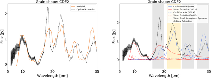
Figure 9. The best-fit model with particle shape calculated with the continuous distribution of ellipsoids (CDE2; Fabian et al. 2001) with quadratic weighting for forsterite grains and enstatite grains. We show the disk spectrum with its featureless blackbody components subtracted from the total flux. Left: model fit (orange) plotted over the data (black). Right: components of different grain species plotted over the data. The flux from all of the grain species (blue and red lines) sums up to the total flux, which equals the model fit (orange) in the left panel.
Download figure:
Standard image High-resolution image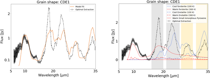
Figure 10. The best-fit model with particle shape calculated with the continuous distribution of ellipsoids (CDE1; Fabian et al. 2001) for forsterite grains and enstatite grains by assuming all shapes are equally probable. We show the disk spectrum with its featureless blackbody components subtracted from the total flux. Left: model fit (orange) plotted over the data (black). Right: components of different grain species plotted over the data. Warm and cool dust species are plotted in red and blue, respectively. Flux from all dust species sums to the model fit (orange) in the left panel.
Download figure:
Standard image High-resolution image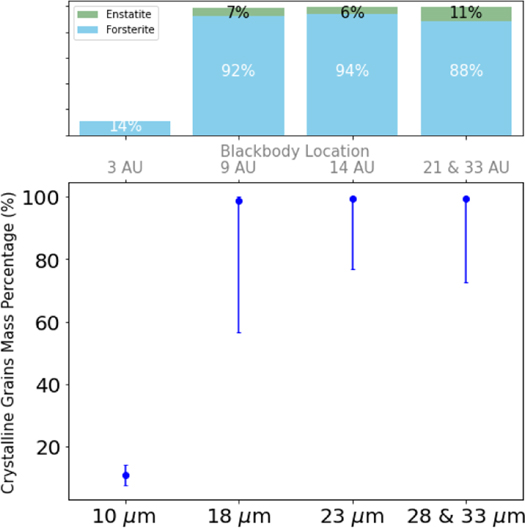
Figure 11. The crystallinity of small silicate grains as a function of radial distance as represented by spectral features emitting at increasing larger disk radii. The y-axis shows the percentage of different grain compositions by mass. The x-axis shows the best-fit models for 10, 18, 23, 28, and 33 μm silicate features. We calculate a blackbody distance at each wavelength by assuming that the grains are blackbodies and in thermal equilibrium such that the incident stellar radiation on a grain equals its thermal re-emission. Note that these distances are lower limits to the actual distances where the grains reside because the grain opacity changes with wavelength, where the blackbody’s opacity does not have a wavelength dependence.
Download figure:
Standard image High-resolution imageThe crystalline fraction in small grains increases from 14 ± 3% at 10 μm (∼3 au) to  % at 18 μm (∼10 au) and remains high from 18 μm (∼10 au) to 33 μm (∼33 au). This sudden increase in grain crystallinity at ∼10 au highlights a major change in the crystallinity of the grain composition. We tabulate the crystallinity fractions in Table 5. Applying these trends to β Pic planetary architecture, we find that the submicron-sized silicate grains exterior to the β Pic b (10 au) are highly crystallized, while the ones interior to β Pic b are mostly amorphous.
Table 5. Fe/Mg Ratio for Crystalline Silicates and Crystallinity Fraction for Grains as a Function of Wavelength
| Quantity | 10 μm | 18 μm | 23 μm | 28 and 33 μm |
|---|---|---|---|---|
| Fe/Mg | 0.05 ± 0.017 | 0.12 ± 0.08 | 0.12 ± 0.05 | 0.11 ± 0.5 |
| Crystallinity (%) | 14 ± 3 |

|

|

|
Download table as: ASCIITypeset image
To understand the abundance of crystalline grains in the β Pic debris disk, we examine their production mechanisms. Two processes produce crystalline grains in a debris disk: (1) Thermal annealing and (2) collisional grinding between parent bodies with crystalline silicate-rich surfaces. Thermal annealing is a process in which amorphous silicates are heated to high temperatures (but below their vaporization temperatures) for enough time that their internal structure rearranges to be crystal-like, producing forsterite, enstatite, and silica (Henning2010). Since thermal annealing is more likely to occur closer to the star, the abundance of crystalline silicates should be the highest closer to the star and decrease with increasing radial distance. However, we find the opposite trend in crystallinity to that predicted by the thermal annealing scenario, which rules out thermal annealing as the main crystallization mechanism. Alternatively, if the surfaces of the parent bodies are crystalline-rich, continuous collisions among these parent bodies can graze off the surface materials and produce grains with high crystallinity. In our solar system, the A-type asteroids in the main asteroid belt are known to have olivine-dominated surfaces based on their reflection spectra (DeMeo et al. 2019). In debris disks, collisional grinding of crystalline-rich parent bodies’ surfaces is also thought to generate enstatite-rich dust grains (Fujiwara et al. 2010; Olofsson et al. 2009). Therefore, the collisional grinding production of crystalline silicates remains a possible production mechanism to explain the crystallinity trend in β Pic.
5.2. The Fe/Mg Abundance Ratio as a Function of Distance
To constrain the formation conditions of the parent bodies in the debris disk, we investigate the Fe/Mg ratio in the crystalline silicates in the disk. We calculate the Fe/Mg ratio by using the silicate masses reported in Table 4 and converting the reported masses into molecular abundance in moles. We then calculate the absolute abundances of Fe and Mg from the stoichiometry of the chemical formulas reported in Table 4. We report the Fe/Mg ratio in Table 5 and plot the Fe/Mg ratio in crystalline silicates as a function of radial distance in Figure 12.
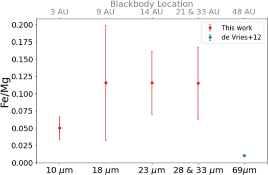
Figure 12. The Fe to Mg ratio for small grains plotted as a function of spectral feature wavelength that can be used as a proxy for stellocentric distance. The red dots with error bars are from this work, and the blue dot is the Fe to Mg ratio measured from Herschel PACS spectra (de Vries et al. 2012).
Download figure:
Standard image High-resolution imageThe Fe/Mg ratio remains constant from 10 to 33 μm, but decreases to less than 1% at 69 μm, when we incorporate the Fe/Mg abundance of (1 ± 0.1)% measured from Herschel/PACS 69 μm forsterite feature (de Vries et al. 2012). Applying this trend to the β Pic planetary architecture, we find that the small dust grains interior to β Pic b (10 au) are more Fe-rich while the dust grains exterior to β Pic b become increasingly Fe-poor. We further discuss the implications of this trend on parent body properties in Sections 6.1 and 6.2.
In addition, we compare β Pic’s Fe/Mg ratio with the Fe/Mg ratio measured from white dwarf atmosphere compositions. Recent measurements of precise elemental abundances from white dwarf atmospheres enable us to probe the compositions of extrasolar rocky planetesimals. Interestingly, we find that our reported Fe/Mg olivine ratio for the 10 μm warm dust is consistent with that of G29-38 (Xu et al. 2014), suggesting that G29-38's rocky planetesimals could contain olivine. We also tabulate the Si, O, Mg, and Fe abundances as a function of radial distance (see Table 6). We find that the abundance of all four species in small grains increases by a factor of 100 from 22 log(Mole) at 10 μm (∼300 K) to 24 log(Mole) at 18 μm (∼160 K).
Table 6. Element Abundance for the Best-fit Models of the β Pic Debris Disk
| Species | 10 μm | 18 μm | 23 μm | 28 and 33 μm |
|---|---|---|---|---|
[ (Mole)] (Mole)] | [ (Mole)] (Mole)] | [ (Mole)] (Mole)] | [ (Mole)] (Mole)] | |
| Si | 22.2 ± 0.7 | 24.3 ± 0.2 | 24.5 ± 0.4 | 24.4 ± 0.4 |
| O | 22.8 ± 0.7 | 24.8 ± 0.2 | 25.1 ± 0.5 | 24.9 ± 0.4 |
| Mg | 22.2 ± 0.7 | 24.5 ± 0.3 | 24.7 ± 0.6 | 24.6 ± 0.5 |
| Fe | 21.9 ± 0.8 | 23.5 ± 0.3 | 23.8 ± 0.6 | 23.6 ± 0.5 |
Download table as: ASCIITypeset image
6. Discussion
6.1. Trends in Silicates and Implications on Parent Body Surface Properties
In Section 5, we report our findings that the submicron-sized silicate grains are increasingly crystalline, Mg-rich (Fe-poor), and irregular in shape as stellocentric distance increases. We highlight that this critical transition in silicate properties occurs in the vicinity of β Pic b’s orbit. As submicron-sized grains must be constantly replenished from planetesimal collisions on orbital timescales, short compared to the age of the disk, these grains reflect the surface composition and conditions of their parent planetesimals.
From the Fe/Mg trend in silicates, we infer that the surfaces of planetesimals interior to β Pic b are more Fe-rich compared to the surfaces of planetesimals exterior to β Pic b. As Fe-bearing silicates are preferentially produced by planetesimal collisions, as we argue in Section 5, the planetesimals close to or interior to β Pic b might have experienced more collisions compared to the planetesimals exterior to β Pic b (outward of 10 au). If the parent planetesimals have not fully differentiated, then the bulk composition of the planetesimals could be increasingly Fe-poor as stellocentric distance increases.
From the crystallinity trend in silicates, we infer that the surfaces of planetesimals interior to β Pic c (∼3 au) are mostly amorphous, while the surfaces of planetesimals exterior to β Pic b are highly crystalline. As crystalline olivine can be easily turned into amorphous olivine via collisions (Henning 2010), the highly crystallized silicate surfaces of planetesimals exterior to β Pic b indicate that these planetesimals have not undergone major collisions.
6.2. Comparing Mineralogy of β Pic and the Solar System
We compare the Fe/Mg gradient of the β Pic chemical reservoir with that observed in the solar system. In the solar system, comets that originate from the trans-Neptunian region contain Mg-rich silicates (Wooden et al. 2017), whereas asteroids and chondrites are Fe-rich (Le Guillou et al. 2015). Such an Fe/Mg trend in the solar system also leaves imprints on terrestrial planetary surfaces. Specifically, most surfaces on Mars contain Fo68, an olivine that is relatively Fe-rich, while ancient craters on Mars contains Fo91, which is relatively Fe-poor; Fo91 is thought to originate from the Kuiper Belt (Hamilton 2010). Therefore, β Pic and the solar system share a similar Fe/Mg trend.
We also compare the olivine grain shape distributions in β Pic with the olivine grain sizes observed in our solar system. In the solar system, submicron-sized forsterite grains are abundant in the chondritic porous interplanetary dust particles (IDP) and comets that originate from the Kuiper Belt (Wozniakiewicz et al. 2012), while much larger and less porous forsterite grains are present in asteroids. In contrast, in the β Pic system, we see submicron forsterite grains throughout the entire disk; their shapes become increasingly irregular as a function of radial distance. Simulations have shown that the fluffy, irregular grain aggregates can produce qualitatively similar spectral features as porous grains (Kolokolova & Kimura 2010). If we consider grain shape a proxy for grain porosity, then the submicron-sized, irregular forsterite grains in the outskirts of β Pic disk correspond to the forsterite grains in our solar system’s comets and IDP.
Our discovery of these similarities paves the way for future space-based spatially resolved MIR spectroscopy studies. Higher spatial resolution observation of the James Webb Space Telescope (JWST) will improve our understanding of β Pic’s planetary system architecture. Future JWST GTO (ID: 1294) observations will be able to probe the spatial distribution of the forsterite population with an improved resolution (by a factor of ∼10 in spatial resolution compared to Spitzer’s spatial resolution) with the MIRI Medium Resolution Spectroscopy as well as a higher overall S/N (compared to ground-based high-resolution observations). The Gemini T-ReCS images revealed an asymmetric dust distribution at 18.3 μm in the disk (Telesco et al. 2005), while the Spitzer discovery provides complimentary spectroscopic information by pinpointing the 18 μm forsterite emission that gives good constraints on grain properties such as Fe/Mg and crystallinity and shape. JWST would be able to map and compare the size, shape, and mass distributions of cool forsterite grains in the southwest and northeast side of the disk, leveraging the knowledge from Gemini and Spitzer. The future JWST MRS observations will also potentially resolve more solid-state emission features and therefore refine measurements of the Fe/Mg and crystallinity ratios for the 18–33 μm features.
6.3. Tentative Evidence for Weak 3–5 μm Hot Dust
In Section 3.4, we showed that a population of ∼600 K hot dust located within 0.7 au likely contributes to ∼50% of excess flux at around 3–5 μm. In comparison, past H- and K-band interferometric measurements indicate a ∼1500 K hot dust population located at least within 4 au of the star (Ertel et al. 2014; Defrére et al. 2012). It is uncertain whether the tentative ∼600 K hot dust is related to the ∼1500 K hot dust population. The ∼600 K hot dust could have multiple origins. Atacama Large Millimeter/submillimeter Array (ALMA) dust continuum images (e.g., Kral et al. 2016) have shown that the inner disk does not have an obvious cavity and can still contain abundant small planetesimals to produce the ∼600 K hot dust. Alternatively, inward P-R drag could operate to move the 10 μm warm dust grains into the inner region of the disk. It is also possible that there are stochastic events in the inner region of the disk, such as comets’ infalling activities (Kiefer et al. 2014), that could produce the ∼600 K hot dust population. Future observations are needed to confirm the tentative ∼600 K hot dust population. β Pic is too bright to be observed by JWST from space but can be observed from the ground. IRTF is a suitable facility for obtaining the 2.5–5 μm NIR spectrum with a high S/N to constrain the level of hot dust excess in this system.
7. Conclusion
We re-analyze the Spitzer IRS data of the β Pic debris disk with AdOpt (Lebouteiller et al. 2010). To better constrain the stellar parameters, we obtained a new NASA IRTF SpeX spectrum from 0.7–3 μm and found a weak 3–5 μm excess possibly due to hot dust close to the star. We discover a prominent 18 μm silicate feature for the first time and an enhanced 23 μm feature. These narrow spectroscopic features placed good constraints on grain properties such as the Fe/Mg ratio, crystallinity, and shape. We find that the ∼100 K forsterite grains are the main contributors to these two features. Furthermore, we find three trends in grain properties as functions of wavelengths: (1) the Fe/Mg ratio in silicates decreases with stellocentric distances. We infer that the surface composition of the planetesimals is increasingly Mg-rich and pristine the farther away they are from the star. We find β Pic’s chemical gradient offers an analogy to our solar system’s clearly divided grain chemical reservoirs; (2) the grains become more crystalline with increasing wavelengths; and (3) lastly, the grain shapes become increasing irregular with increasing wavelengths. The findings imply that the properties of the dust population in the vicinity of β Pic b and c differ significantly in crystallinity, shape, and Fe/Mg ratio. This is the first time that such a trend in spectral features has been studied with space-based MIR spectroscopy for a debris disk. Future JWST MIRI observations will constrain the spatial location of the grains that are responsible for the newly discovered 18 and 23 μm spectral features and probe β Pic b’s atmospheric cloud composition for comparison with dust properties in the planet’s vicinity.
We thank Alycia Weinberger, Benjamin Montesinos, Francisca Kemper, John Debes, Roc Cutri, Bin Ren, and Jingwen Fan for useful discussions. C.L. acknowledges support from the STScI Director’s Discretionary Fund and NASA through the FINESST program (Award No. 80NSSC21K1844). This work is supported by the National Aeronautics and Space Administration under grant No. 80NSSC21K1844 issued through the Mission Directorate. This work is based on archival data obtained with the Spitzer Space Telescope, which was operated by the Jet Propulsion Laboratory, California Institute of Technology under a contract with NASA. This research has made use of the NASA/IPAC Infrared Science Archive, which is funded by the National Aeronautics and Space Administration and operated by the California Institute of Technology. This publication makes use of data products from the Wide-field Infrared Survey Explorer, which is a joint project of the University of California, Los Angeles, and the Jet Propulsion Laboratory/California Institute of Technology, and NEOWISE, which is a project of the Jet Propulsion Laboratory/California Institute of Technology. WISE and NEOWISE are funded by the National Aeronautics and Space Administration. This research has made use of NASA’s Astrophysics Data System. This research has made use of the SIMBAD database, operated at CDS, Strasbourg, France (Wenger et al. 2000). This research has made use of the VizieR catalog access tool, CDS, Strasbourg, France (DOI: 10.26093/cds/vizier). The original description of the VizieR service was published in 2000, A&AS 143, 23 (Ochsenbein et al. 2000).
Appendix: Spitzer IRS Spectrograph Slit Orientation
We showcase the misalignment angle between the LL slit position angle (PAslit = 44.97 ± 0.02°) and disk midplane PA (PAdisk = 29.51°) by overlaying IRS LL2 slit on top of the data for a visualization (as mentioned in Section 2.2.1).
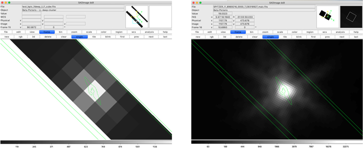
Figure A1. The β Pic debris disk in the slit of IRS spectrograph. The coordinate display here is the world coordinate system, in which north points upwards and east points to the left. The green contour shows the disk of β Pic in scattered light, and is obtained from the scattered-light image with the Space Telescope Imaging Spectrograph on the Hubble Space Telescope (Ren et al. 2017; see Figure 6(c) therein). The southwest side of the disk contains gas clumps as seen in ALMA. The disk is measured to have a position angle of PAdisk = 2951. The edges of the IRS spectrograph slit are indicated by the green lines (we zoomed in to show part of the slit, since the entire slit is too long). The slit has a position angle of PAslit = 44.97 ± 0
02. The disk is 15° misaligned with respect to the slit. Left: the mosaic image in the background is the β Pic 2D spectral map taken with IRS long-low 1 (LL1) mode and assembled using Cubism (Sings IRS Team et al. 2011). Shown here is the disk at 20.52 μm, and there are 100 other slices (not shown here) in LL1 that span λ ∼ 20–39 μm in wavelength. The disk roughly spans 2.5 pixels in this image, and each pixel is square with 5.1″ on each side. Right: the background image is taken with the Spitzer MIPS 24 μm image. The image pixel has a size of 2
49 × 2
60. We use MIPS photometry for absolute flux calibration for the IRS spectrum.
Download figure:
Standard image High-resolution imageFootnotes
- 12
For forsterite and enstatite, we leave their exact stoichiometry for a discussion in the next paragraph.
- 13
Here we use the Fo notation, where Fo stands for the percentage of Fe in forsterite stoichiometry. Fo100 represents the magnesium-rich end-member of olivine, forsterite (Mg2SiO4) with 100% Mg and 0% Fe, and Fo0 represents the Fe-rich end-member of olivine, fayalite (Fe2SiO4, known as Fa), with 100% Fe and 0% Mg. For example, Fo80 represents 80% Mg and 20% Fe. The same convention is used to describe the enstatite stoichiometry.