Abstract
Using 2D particle-in-cell (PIC) simulations, the generation of electrostatic solitary waves (ESWs) and the associated plasma waves in symmetric magnetic reconnection are studied, and multiple kinds of ESWs with different propagating speeds are identified. Near the current sheet in the outflow region, there are two kinds of ESWs propagating away from the X line: their propagating speeds are about 0.73VTe0 and 1.2VTe0 (where VTe0 is the initial electron thermal velocity), and their generation is associated with the Buneman instability and the electron two-stream instability, respectively. In the separatrix region, there is one kind of ESW propagating toward the X line with a propagating speed of about 1.2 VTe0, which is formed during the nonlinear evolution of the electron two-stream instability. We also run a case with a guide field, and there exist two kinds of ESWs: the ESWs propagating away from the X line can be generated near the separatrices with electron outflow, while the ESWs propagating toward the X line can be generated near the separatrices with electron inflow. The two kinds of ESWs are associated with the electron two-stream instability and the Buneman instability, respectively.
Original content from this work may be used under the terms of the Creative Commons Attribution 4.0 licence. Any further distribution of this work must maintain attribution to the author(s) and the title of the work, journal citation and DOI.
1. Introduction
Electrostatic solitary waves (ESWs) are one kind of highly nonlinear structures in collisionless plasma, which are often interpreted as electron phase-space holes (electron holes or EHs) with electron trapping (Bernstein et al. 1957; Roberts & Berk 1967; Ng & Bhattacharjee 2005; Wu et al. 2011; Hutchinson 2017). These Debye-scale waves have bipolar parallel electric fields, presenting a positive potential structure (Matsumoto et al. 1994; Krasovsky et al. 1997; Mangeney et al. 1999; Franz et al. 2000; Lu et al. 2005b; Steinvall et al. 2019). Kinetic simulations have demonstrated that ESWs are produced in the nonlinear stage of various plasma instabilities related to electron beams (Omura et al. 1994, 1996; Lu et al. 2005a; Umeda et al. 2006; Lu et al. 2008; Norgren et al. 2015). The first instability is the electron two-stream instability, where the densities of the two streams are comparable and the propagating velocity of the resulting ESWs is between the drift velocities of the two streams (Omura et al. 1994, 1996; Lu et al. 2008). The second one is the electron bump-on-tail instability, where the density of the background electron component is much larger than that of the electron beam. The propagating velocity of ESWs generated by the electron bump-on-tail instability is almost the same as the drift velocity of the electron beam (Omura et al. 1996; Umeda et al. 2002; Lu et al. 2005a). The third one is the Buneman instability, which is generated because of the relative drift between ion and electron components, and the propagating velocity of the ESWs is between the drift velocity of ion and electron components and is closer to the ion drift velocity (Omura et al. 1994; Norgren et al. 2015). Satellite observations have shown that besides these kinds of ESWs excited by instabilities related to electron beams, the acoustic instability and the lower hybrid instability can also lead to the generation of ESWs (Steinvall et al. 2021).
Magnetic reconnection, where magnetic energy is dissipated into plasma kinetic energy via the topological change of magnetic field lines (Parker 1957; Vasyliunas 1975; Lu et al. 2013; Burch et al. 2016; Shu et al. 2021), is believed to be responsible for various phenomena in the space plasma, such as magnetospheric substorms and solar flares. Electrons can be accelerated during magnetic reconnection, and electron beams are consequently formed (Nagai et al. 2001; Pritchett 2001; Lu et al. 2010). Electrostatic waves associated with beam instabilities can be converted to electromagnetic emissions through wave–wave coupling, which is a widely accepted mechanism of type III solar radio bursts (Schmitz & Tsiklauri 2013; Yao et al. 2021). Electron beams in reconnection may also generate ESWs. Actually, satellite observations and numerical simulations have demonstrated the existence of ESWs in the vicinity of the X line (Drake et al. 2003; Yu et al. 2021), the separatrix region (Matsumoto et al. 2003; Pritchett & Coroniti 2004; Cattell et al. 2005; Fujimoto & Machida 2006; Retinò et al. 2006; Lapenta et al. 2010), and the jet front of magnetic reconnection (Deng et al. 2010; Liu et al. 2019). Satellite observations have also revealed the close relation between ESWs and electron beams in magnetic reconnection (Yu et al. 2021). Drake et al. (2003) used an initial force-free equilibrium of current sheet with a strong guide field in a 3D particle-in-cell (PIC) simulation of magnetic reconnection and found that the Buneman instability, unstable to the initially imposed interaction between ions and electrons, can produce ESWs near the X line. Numerous PIC simulations have shown that the ESWs in the separatrix region are related to electron beams. During antiparallel reconnection, Fujimoto & Machida (2006) considered that the ESWs in the separatrix region propagating to the downstream direction are generated by the electron two-stream instability, while Huang et al. (2014) attributed them to the electron bump-on-tail instability. In magnetic reconnection with a guide field, Lapenta et al. (2010) and Divin et al. (2012) found that ESWs in the separatrix region propagating to the X line are produced by the Buneman instability.
Recently, both in situ satellite observations and kinetic simulations indicated that multiple kinds of ESWs with distinct propagating velocities may coexist near the reconnection separatrices (Graham et al. 2015, 2016; Chang et al. 2021). Graham et al. (2015) found that ESWs have different length scales and propagating velocities in the same asymmetric magnetopause reconnection event. Detailed analysis showed that these various kinds of ESWs may be related to the electron two-stream instability, the bump-on-tail instability, or the Buneman instability (Graham et al. 2015, 2016). By analyzing the wave characteristics in asymmetric reconnection, Chang et al. (2021) showed that the same electron beam can drive both the Buneman instability and the electron two-stream instability in the separatrix region with electron outflow and lead to two kinds of ESWs propagating away from the X line. Besides the magnetopause, magnetic reconnection can also occur in the magnetotail. The plasma parameters across the magnetotail current sheet are almost the same, and magnetic reconnection is symmetric. By performing a 2D PIC simulation of symmetric reconnection, Fujimoto (2014) found the existence of two kinds of ESWs around the separatrices propagating toward the X line: at the region far away from the X line, the speed of the electron beam is relatively weak and the ESWs are excited by the Buneman instability, while at the region closer to the X line, the ESWs are excited by the electron two-stream instability. Satellite observations of magnetotail reconnection exhibited that ESWs tend to propagate away from the X line near the plasma sheet and toward the X line near the lobe region (Li et al. 2014). This motivates us to perform a 2D PIC simulation of symmetric reconnection, with the focus on the excitation of various kinds of plasma waves in the separatrix region, and to analyze the detailed characteristics of the consequently generated ESWs, including propagating directions and velocities.
2. Simulation Model
In the PIC simulation model, given the initial configuration of electric and magnetic fields, as well as the spatial and velocity distributions of particles, the particle motions and electromagnetic fields are closely coupled. The electric and magnetic fields are updated by solving Maxwell equations with an explicit leapfrog algorithm, and the particle motions are calculated by the Newton–Lorentz equations. In this paper, a 2D PIC simulation code is used.
The initial configuration is a 2D Harris current sheet with magnetic field  , where B0 and By0 are the asymptotic magnetic field and initial guide field, respectively, and δ is the half-width of the current sheet. The plasma density is
  , where n0 is the peak density of the current sheet and the background density is nb
= 0.1n0. We set δ = 0.5di
(where di
= c/ωpi
denotes the ion inertial length defined by n0), mi
/me
= 100 (where mi
denotes ion mass and me
denotes electron mass), and c = 15VA (where c denotes the light speed and
, where n0 is the peak density of the current sheet and the background density is nb
= 0.1n0. We set δ = 0.5di
(where di
= c/ωpi
denotes the ion inertial length defined by n0), mi
/me
= 100 (where mi
denotes ion mass and me
denotes electron mass), and c = 15VA (where c denotes the light speed and  is the Alfvén speed). The distribution functions of ions and electrons are Maxwellian, and the initial temperature ratio is set to be Ti0/Te0 = 4 (where Ti0 is initial temperature of ions and Te0 is the initial temperature of electrons). The velocities are expressed in units of the initial electron thermal velocity
  , and VTe0/VA = 4.5. The grid number is Nx
× Nz
= 1600 × 400, and the grid size is Δx = Δz = 0.05di
. The time step is
, and VTe0/VA = 4.5. The grid number is Nx
× Nz
= 1600 × 400, and the grid size is Δx = Δz = 0.05di
. The time step is  (where Ωi
= eB0/mi
is the ion gyrofrequency). In the z-direction, conducting boundary conditions are employed, while periodic boundary conditions are employed in the x-direction. In order to trigger magnetic reconnection quickly, a small magnetic flux perturbation is given as
(where Ωi
= eB0/mi
is the ion gyrofrequency). In the z-direction, conducting boundary conditions are employed, while periodic boundary conditions are employed in the x-direction. In order to trigger magnetic reconnection quickly, a small magnetic flux perturbation is given as  and ψ0 = 0.05 cB0/ωpi
.
and ψ0 = 0.05 cB0/ωpi
.
3. Simulation Results
In this paper, we run two cases to investigate the excitation of ESWs in magnetic reconnection. In Run 1 we use the current sheet without an initial guide field, and in Run 2 we use the current sheet with an initial guide field By0/B0 = − 1.0.
Figures 1(a) and (b) plot the parallel electric field E∣∣ and parallel electron bulk velocity Ve∣∣ (where E∣∣ = E • B /∣B∣, Ve∣∣ = V e • B /∣B∣) at Ωi t = 23 for Run 1. In the regions near the separatrices, electrons flow toward the X line along the magnetic field lines, while electrons flow away from the X line in the outflow regions. From the figure, we can identify simultaneously three kinds of ESWs with the bipolar structure of E∣∣. Detailed analysis shows that there are two kinds of ESWs propagating away from the X line and one kind of ESW propagating toward the X line. The ESWs propagating away from the X line are situated downstream of the dipolarization fronts and can be observed far away from the reconnection region. The bipolar structures of E∣∣ propagating away from the X line begin to appear at about Ωi t = 18, while the bipolar structures propagating toward the X line are formed later and appear at about Ωi t = 23. The propagation of these ESWs is exhibited in the supplementary animation.
Figure 1. The (a) parallel electric field E∣∣ and (b) parallel electron bulk velocity Ve∣∣, normalized by the initial electron thermal velocity  (where E∣∣ =
E
•
B
/∣B∣, Ve∣∣ =
V
e
•
B
/∣B∣) at Ωi
t = 23 for Run 1. Two typical bipolar structures with slower and faster velocities moving away from the X line are denoted as “OUT-S” and “OUT-F,” respectively. A bipolar structure moving toward the X line with fast speed is denoted as “IN-F.” Here the magnetic field lines and separatrices are represented by solid and dashed curves, respectively. An animation of Figure 1(a) is available. The animation starts at Ωi
t = 18 and ends at Ωi
t = 24, and the time interval is
(where E∣∣ =
E
•
B
/∣B∣, Ve∣∣ =
V
e
•
B
/∣B∣) at Ωi
t = 23 for Run 1. Two typical bipolar structures with slower and faster velocities moving away from the X line are denoted as “OUT-S” and “OUT-F,” respectively. A bipolar structure moving toward the X line with fast speed is denoted as “IN-F.” Here the magnetic field lines and separatrices are represented by solid and dashed curves, respectively. An animation of Figure 1(a) is available. The animation starts at Ωi
t = 18 and ends at Ωi
t = 24, and the time interval is  . The bipolar structures propagating away from the X line begin to appear at about Ωi
t = 18 and are situated downstream of the dipolarization fronts, while the bipolar structures propagating toward the X line are formed later and are located in the separatrix region. The total, real-time duration of the animation is 14 s.Animationmp=4
. The bipolar structures propagating away from the X line begin to appear at about Ωi
t = 18 and are situated downstream of the dipolarization fronts, while the bipolar structures propagating toward the X line are formed later and are located in the separatrix region. The total, real-time duration of the animation is 14 s.Animationmp=4
(An animation of this figure is available.)
Download figure:
Video Standard image High-resolution imageThe simultaneous existence of various kinds of ESWs is shown in Figure 2, which exhibits the distribution of E∣∣ in the region 44di ≤ x ≤ 64di , −4.5di ≤ z ≤ 0 at (a) Ωi t = 21.2, (b) Ωi t = 21.8, (c) Ωi t = 22.4, (d) Ωi t = 23.0, and (e) Ωi t = 23.6 for Run 1. In the reconnection outflow region, there are two kinds of ESWs propagating away from the X line. Two typical bipolar structures selected from the two kinds of ESWs are denoted as “OUT-S” and “OUT-F,” and they move away from the X line along the magnetic field lines. The bipolar structure “OUT-F” lags behind “OUT-S” at Ωi t = 21.2; however, it catches up with “OUT-S” at about Ωi t = 21.8 and then overtakes “OUT-S.” The propagating speed of the bipolar structure “OUT-F” is faster than that of “OUT-S.” At about Ωi t = 23.0, a bipolar structure denoted as “IN-F” appears in the separatrix region, and it propagates toward the X line along the magnetic field. In the figure, we only plot the ESWs around the lower right separatrix, while those around other separatrices are almost the same.
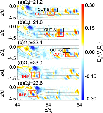
Figure 2. The distributions of the parallel electric field E∣∣ within 44di ≤ x ≤ 64di , −4.5di ≤ z ≤ 0 at Ωi t = 21.2, (b) Ωi t = 21.8, (c) Ωi t = 22.4, (d) Ωi t = 23.0, and (e) Ωi t = 23.6 for Run 1. Two typical bipolar structures with slower and faster velocities moving away from the X line are denoted as “OUT-S” and “OUT-F.” A bipolar structure moving toward the X line with fast speed is denoted as “IN-F.”
Download figure:
Standard image High-resolution imageIn Figure 3(a), we plot the distribution of E∣∣ within 52di
≤ x ≤ 72di
, −4.5di
≤ z ≤ 0 at Ωi
t = 22 for Run 1. Then, in Figures 3(b)–(c) we show the electron distributions in the x − ve∣∣ space along the red dashed lines in Figure 3(a). Figure 4(a) describes the distribution of E∣∣ in the region 46di
≤ x ≤ 54di
, −4.5di
≤ z ≤ 0 at Ωi
t = 23 for Run 1, and Figures 4(b) and (c) exhibit the profile of E∣∣ and the electron distribution in the x − ve∣∣ space along the magnetic field line  (indicated by the red dashed line in Figure 4(a)). Figures 3 and 4 describe the characteristics of the ESWs moving away from and toward the X line, respectively. Obviously, every bipolar structure of parallel electric field corresponds to one electron hole in the x − ve∣∣ space. Thus, the generated ESWs may be consistent with the BGK mode (Ng & Bhattacharjee 2005; Huang et al. 2014). With the periodic boundary conditions used in the simulation, some high-speed electrons are able to cross the boundary at the late stage of reconnection. We have confirmed that our analyses are not affected by these electrons.
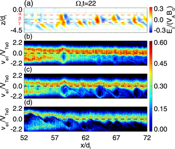
Figure 3. (a) The distribution of the parallel electric field E∣∣ within 52di ≤ x ≤ 72di , −4.5di ≤ z ≤ 0 at Ωi t = 22 for Run 1. Panels (b)–(d) show the electron distributions in the x − ve∣∣ space along the red dashed lines indicated by α, β, and γ in panel (a), respectively.
Download figure:
Standard image High-resolution image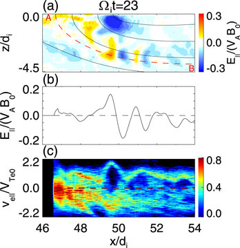
Figure 4. (a) The distribution of the parallel electric field E∣∣ within 46di
≤ x ≤ 54di
, −4.5di
≤ z ≤ 0 at Ωi
t = 23 for Run 1. (b) The profile of E∣∣ and the electron distribution in the x − ve∣∣ space along a magnetic field line indicated by  .
.
Download figure:
Standard image High-resolution imageFigures 5(a)–(c) show the time evolution of E∣∣ along red dashed lines in Figure 3(a) from Ωi
t = 21 to 27 for Run 1. These ESWs move away from the X line. There is only one kind of ESW along the lines α and γ, and their propagating speeds are estimated to be about 0.73VTe0 and 1.2VTe0, respectively. Both kinds of ESWs can exist along the line β. Figure 6 presents the time evolution of E∣∣ along the dashed line denoted by  in Figure 4(a). The ESWs propagate toward the X line with a speed of about 1.2 VTe0.
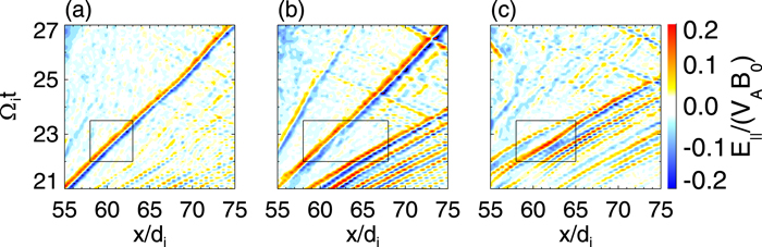
Figure 5. The time evolution of the parallel electric field E∣∣ along (a) z = − 1.3di (the red dashed line indicated by α in Figure 3), (b) z = − 2.0di (the red dashed line indicated by β in Figure 3), and (c) z = − 2.7di (the red dashed line indicated by γ in Figure 3) from Ωi t = 21 to 27 for Run 1.
Download figure:
Standard image High-resolution image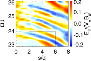
Figure 6. The time evolution of E∣∣ along the magnetic field line indicated by  in Figure 4(a) from Ωi
t = 23 to 26 for Run 1. The origin of the s axis is point A (the intersection between the magnetic field line
in Figure 4(a) from Ωi
t = 23 to 26 for Run 1. The origin of the s axis is point A (the intersection between the magnetic field line  and z = 0).
Download figure:
Standard image High-resolution imageIn order to identify the plasma instabilities generating these ESWs in our PIC simulation of magnetic reconnection, we analyze the electron and ion velocity distributions in the regions with ESWs. Figures 7(a)–(c) show the parallel velocity distributions of electrons f(ve∣∣) and ions f(vi∣∣) within (a) 57.5di ≤ x ≤ 58.0di , −1.6di ≤ z ≤ − 1.0 di , (b) 58.0di ≤ x ≤ 58.5di , −2.3di ≤ z ≤ − 1.7di , and (c) 58.5di ≤ x ≤ 59.0di , −3.0di ≤ z ≤ − 2.4di at Ωi t = 22 for Run 1. The ion distributions can be fitted well by a Maxwellian function without an obvious bulk velocity. The electron distributions can be considered to consist of two components, and each component is fitted well with a Maxwellian function. The first electron component is the electron inflow moving toward the X line along the separatrices, while the second electron component is the electron outflow. The fitting parameters are listed in Table 1. The bulk velocities of the first electron component are about 0.73 VTe0, 0.76 VTe0, and 0.53 VTe0, and the bulk velocities of the second electron component are about −1.34 VTe0, −1.41 VTe0, and −1.41 VTe0 in these regions.
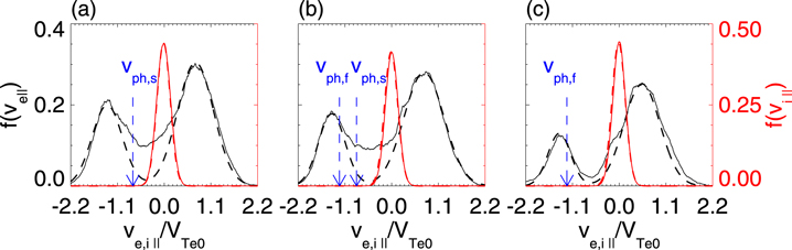
Figure 7. The parallel velocity distributions of electrons f(ve∣∣) (black) and ions f(vi∣∣) (red) within (a) 57.5di ≤ x ≤ 58.0di , −1.6di ≤ z ≤ − 1.0di , (b) 58.0di ≤ x ≤ 58.5di , −2.3di ≤ z ≤ − 1.7di , and (c) 58.5di ≤ x ≤ 59.0di , −3.0di ≤ z ≤ − 2.4di at Ωi t = 22 for Run 1. The velocity distributions fitting with the Maxwellian function are represented by the dashed lines. The blue arrows indicate the phase speeds at the maximum growth rate of the electron two-stream instability (“vph,f ”) and the Buneman instability (“vph,s ”), respectively.
Download figure:
Standard image High-resolution imageTable 1. Fitting Parameters of Electron and Ion Velocity Distribution
| Figure 7(a) | Figure 7(b) | Figure 7(c) | Figure 9 | |
|---|---|---|---|---|
| Ve1/VTe0 | 0.73 | 0.76 | 0.53 | 1.1 |
| Ve2/VTe0 | −1.34 | -1.41 | −1.41 | −1.3 |
| Vi /VTe0 | −0.02 | -0.02 | −0.02 | −0.01 |
| Vte1/VTe0 | 0.43 | 0.47 | 0.43 | 0.3 |
| Vte2/VTe0 | 0.36 | 0.31 | 0.27 | 0.67 |
| Vti /VTe0 | 0.16 | 0.16 | 0.16 | 0.16 |
| ne1/ni | 0.64 | 0.70 | 0.75 | 0.27 |
| ne2/ni | 0.36 | 0.30 | 0.25 | 0.73 |
Note. Ve1 (Vte1) and Ve2 (Vte2) are the bulk velocities (thermal velocities) of the first and second electron component, and Vi (Vti ) is the bulk velocity (thermal velocity) of the ion component. We normalize the bulk velocities and the thermal velocities of electrons and ions based on the initial electron thermal velocity VTe0. ne1 and ne2 are the number densities of the first and second electron components, respectively, and both are normalized by the local ion number density ni .
Download table as: ASCIITypeset image
According to these parameters, both the Buneman instability and the electron two-stream instability are unstable. Their dispersion relations (ω, k) and the growth rates (γ) deduced from the electrostatic dispersion relation are plotted in Figures 8(a)–(c). We also plot the wave spectra obtained by the Fourier transform of E∣∣ within (a) 58di
≤ x ≤ 63di
(at z = − 1.3di
), (b) 58.5di
≤ x ≤ 68.5di
(at z = − 2.0di
), (c) 59di
≤ x ≤ 66di
(at z = − 2.7di
), and the time interval 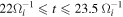 (the black boxes in Figure 5). In Figure 8(a), the power spectral density of E∣∣ has only one peak around (ω/ωpe
, kde
) ∼ (0.045, 0.2). The simulation result is consistent with the theoretical profile of the Buneman instability, that is, the spectral peak is located near the wavenumber with the maximum growth rate obtained from the dispersion relation. By comparing the wave spectra with the calculated dispersion relations and growth rates, we can easily find that in Figures 8(a) and (c) the formed ESWs correspond to the Buneman instability and the electron two-stream instability. In Figure 8(b), both the Buneman instability and the electron two-stream instability are unstable, which leads to the coexistence of two kinds of ESWs.
(the black boxes in Figure 5). In Figure 8(a), the power spectral density of E∣∣ has only one peak around (ω/ωpe
, kde
) ∼ (0.045, 0.2). The simulation result is consistent with the theoretical profile of the Buneman instability, that is, the spectral peak is located near the wavenumber with the maximum growth rate obtained from the dispersion relation. By comparing the wave spectra with the calculated dispersion relations and growth rates, we can easily find that in Figures 8(a) and (c) the formed ESWs correspond to the Buneman instability and the electron two-stream instability. In Figure 8(b), both the Buneman instability and the electron two-stream instability are unstable, which leads to the coexistence of two kinds of ESWs.
Figure 8. Wave spectra of E∣∣ within (a) 58di
≤ x ≤ 63di
(at z = − 1.3di
), (b) 58.5di
≤ x ≤ 68.5di
(at z = − 2.0di
), (c) 59di
≤ x ≤ 66di
with time interval  (at z = − 2.7di
) (the black boxes in Figure 5) for Run 1. The theoretical dispersion relations (dashed curves) and growth rates (solid curves) based on the electron two-stream instability (black) and the Buneman instability (red) are plotted for reference.
(at z = − 2.7di
) (the black boxes in Figure 5) for Run 1. The theoretical dispersion relations (dashed curves) and growth rates (solid curves) based on the electron two-stream instability (black) and the Buneman instability (red) are plotted for reference.
Download figure:
Standard image High-resolution imageFigure 9 shows the electron parallel velocity distribution f(ve∣∣) and ion parallel velocity distribution f(vi∣∣) in the region 51di
≤ x ≤ 51.5di
, −4.0di
≤ z ≤ − 3.4di
at Ωi
t = 23 for Run 1. Similar to Figure 7, the ion distribution can be fitted by a Maxwellian function without an obvious bulk velocity, and the electron distribution consists of two Maxwellian components. The fitting parameters are listed in Table 1. The bulk velocities of the first and second electron components are about 1.1VTe0 and −1.3 VTe0, respectively. With the same method, we can calculate the dispersion relations and growth rates of both the Buneman instability and the electron two-stream instability, which are plotted in Figure 10. By comparing them with the wave spectrum obtained by the Fourier transform of E∣∣ within 2di
≤ s ≤ 6di
,  (the black box in Figure 6), we can know that the ESWs are formed by the electron two-stream instability.
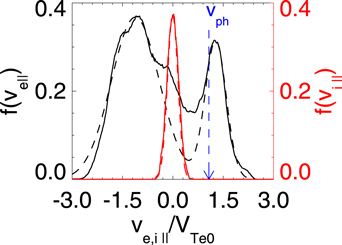
Figure 9. The parallel velocity distributions of electrons f(ve∣∣) (black) and ions f(vi∣∣) (red) within 51di ≤ x ≤ 51.5di , −4.0di ≤ z ≤ − 3.4di at Ωi t = 23 for Run 1. The velocity distributions fitting with the Maxwellian function are represented by the dashed lines. The blue arrow indicates the phase speed at the maximum growth rate of the electron two-stream instability.
Download figure:
Standard image High-resolution image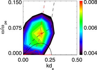
Figure 10. Wave spectrum of E∣∣ within 2di
≤ s ≤ 6di
 (the black box in Figure 6) for Run 1. The theoretical dispersion relations (dashed curves) and growth rates (solid curves) based on the electron two-stream instability (black) and the Buneman instability (red) are plotted for reference.
Download figure:
Standard image High-resolution imageIn Run 2, the characteristics of ESWs during guide field reconnection are investigated. Figures 11(a) and (b) plot the parallel electric field E∣∣ and parallel electron bulk velocity Ve∣∣ at Ωi t = 24 for Run 2. ESWs can be generated around the separatrix regions. Electron inflows appear near the upper left and lower right separatrices, where the ESWs move toward the X line along the magnetic field with a speed of about 0.8 VTe0. The ESWs near the separatrices with electron inflow are generated as a result of the Buneman instability. Electron outflows appear near the lower left and upper right separatrices, where the ESWs move away from the X line with a speed of about 1.0VTe0. The ESWs near the separatrices with electron outflow are excited by the electron two-stream instability.
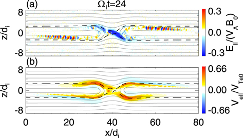
Figure 11. The (a) parallel electric field E∣∣ and (b) parallel electron bulk velocity Ve∣∣ at Ωi t = 24 for Run 2. Here magnetic field lines and separatrices are represented by solid and dashed curves, respectively.
Download figure:
Standard image High-resolution image4. Conclusions and Discussion
In summary, with 2D PIC simulations, we investigate the characteristics of ESWs in symmetric magnetic reconnection and find that multiple kinds of ESWs can be simultaneously formed around the separatrices. In Run 1 without an initial guide field, there are two kinds of ESWs moving away from the X line near the current sheet in the outflow region, and their propagating speeds are about 0.73 VTe0 and 1.2 VTe0. The slower one corresponds to the Buneman instability, and the faster one results from the electron two-stream instability. In the separatrix region, there is one kind of ESW propagating toward the X line with a propagating speed of about 1.2 VTe0. The ESWs propagating toward the X line are generated by the electron two-stream instability. In Run 2 with an initial guide field, the ESWs propagating toward the X line can be generated near the separatrices with electron inflow, and the ESWs propagating away from the X line can be generated near the separatrices with electron outflow, and they are associated with the Buneman instability and the electron two-stream instability, respectively.
In our simulations, the ion-to-electron mass ratio is set to 100. In the case of a realistic mass ratio, the spatial size of the ESWs will be changed, and the parallel electric field strength in the electron holes is found to be suppressed (Lapenta et al. 2010). Furthermore, the phase velocities of the ESWs generated by electron-beam instabilities are also affected by the mass ratio because the mass ratio will change the generated electron-beam velocity and then the phase velocities of the ESWs. However, the phase velocities normalized by the initial electron thermal velocity, as presented in this paper, change little in the case of different mass ratios. Therefore, our main conclusions are expected to be valid in the case of a realistic mass ratio.
Multiple kinds of ESWs with different propagating speeds have been simultaneously observed in magnetic reconnection, which are suggested to correspond to different plasma instabilities. The fast-propagating ESWs are considered to be formed by the electron two-stream instability or the electron bump-on-tail instability, while the slow ESWs are formed by the Buneman instability (Graham et al. 2015, 2016). In this paper, with PIC simulations, we verified that multiple kinds of ESWs can simultaneously exist in magnetic reconnection. The electron beams are generated in the separatrix region and then excite electrostatic instabilities: the electron two-stream instability and the Buneman instability. We further identified that both the fast and slow ESWs propagating away from the X line can coexist near the current sheet in the outflow region, while there only exist fast ESWs propagating toward the X line in the separatrix region. Our results provide theoretical support for these observations. With PIC simulations of guide field reconnection, Lapenta et al. (2010) and Divin et al. (2012) also showed that ESWs can be generated near the four separatrices. The formation of the ESWs near the separatrices with electron inflow propagating to the X line is attributed to the Buneman instability. In our study, besides the ESWs produced near the separatrices with electron inflow by the Buneman instability, we further demonstrate that the ESWs near the separatrices with electron outflow result from the electron two-stream instability.
This work was supported by the Fundamental Research Funds for the Central Universities WK2080000164, WK3420000017, and KY2080000088; the NSFC grant 42174181; the Key Research Program of Frontier Sciences CAS (QYZDJ-SSW-DQC010); and the Strategic Priority Research Program of Chinese Academy of Sciences, grant No. XDB41000000.