Abstract
We present a census of photometrically detected rotation periods for white dwarf (WD) stars. We analyzed the light curves of 9285 WD stars observed by the Transiting Exoplanet Survey Satellite up to Sector 69. Using Fourier transform analyses and the TESS_localize software, we detected variability periods for 318 WD stars. The 115 high-probability likely single WDs in our sample have a median rotational period of 3.9 hr and a median absolute deviation of 3.5 hr. Our distribution is significantly different from the distribution of the rotational period from asteroseismology, which exhibits a longer median period of 24.2 hr and a median absolute deviation of 12.1 hr. In addition, we reported nonpulsating periods for three known pulsating WDs with rotational periods previously determined by asteroseismology: NGC 1501, TIC 7675859, and G226-29. We also calculated evolutionary models including six angular momentum transfer mechanisms from the literature throughout evolution in an attempt to reproduce our findings. Our models indicate that the temperature–period relation of most observational data is best fitted by models with low metallicity, probably indicating problems with the computations of angular momentum loss during the high-mass-loss phase. Our models also generate internal magnetic fields through the Tayler–Spruit dynamo.
Original content from this work may be used under the terms of the Creative Commons Attribution 4.0 licence. Any further distribution of this work must maintain attribution to the author(s) and the title of the work, journal citation and DOI.
1. Introduction
The rotation period is an essential parameter for the study of stellar evolution. It plays a significant role in the stellar dynamo mechanism and is directly related to the mass loss experienced by stars during the asymptotic giant branch (AGB; e.g., Dominguez et al. 1999; Catalán et al. 2008; Romero et al. 2015; Choi et al. 2016). For single stars and stars in binary systems, photometry allows us to detect the rotation period of stars directly and indirectly through asteroseismology (e.g., Córsico et al. 2019).
Depending on the geometry of the system and the orientation of the orbital plane as observed from Earth, binary stellar systems can exhibit light variability due to different effects. All variabilities resulting from the orbital motion of binary systems—ellipsoidal variation, reflection, or eclipses—indicate the system’s orbital period or a harmonic (e.g., Krtička et al. 2023). However, in the case of spin–orbit coupling, there is no difference between the orbital and rotational periods. The spin–orbit coupling occurs when there is mass loss due to winds, trying to balance the variation in the spin of each star with the angular momentum of the system. Zahn (1977) demonstrated that the synchronization time between stellar rotation and the orbital period of a binary system is proportional to  , where Porb is the orbital period of the system. This implies that the shorter the orbital period, the faster the synchronization process occurs. Zahn (1977) suggests that systems with orbital periods shorter than 17 days are synchronized. On the other hand, for compact stars such as white dwarfs (WDs), Fuller & Lai (2011), Pablo et al. (2012), Fuller & Lai (2013), Fuller (2017), and Fuller & Mathis (2023) estimate that synchronization may occur only for orbital periods of the order of 1 hr.
Single stars, such as the Sun, may also exhibit light variability because of the presence of dark spots and patches on their surface. These inhomogeneities are typically associated with the presence of a magnetic field or with a variation in the chemical composition across the stellar surface (e.g., Babcock 1960; Kochukhov 2011). In this case, the rotation period as well as some harmonics can be present in the frequency spectrum, depending on the number of spots.
WD stars are the most common end of stellar evolution, constituting the fate of 95%–97% of all stars in the Galaxy (e.g., García-Berro et al. 1997; Poelarends et al. 2008; Siess 2010; Langer 2012; Doherty et al. 2014; Woosley & Heger 2015). As fossils, WDs preserve valuable information about their past evolution, making them essential for studying the structure, evolution, chemical enrichment, and star formation history of our Galaxy (Diaz-Pinto et al. 1994). WDs are classified into spectral classes based on the dominant chemical element on their surface. Approximately 80% of all WDs belong to the DA spectral type (e.g., Kepler et al. 2021); that is, they exhibit H-dominated spectra. The remaining 20% consist mainly of WD stars of the spectral types DB and DO, featuring helium-dominated atmospheres. When the spectral type is followed by a “V” it means that the star is variable. Thus, for instance, a DAV is a variable WD with H-dominated spectra.
Although WDs have been studied since 1915 (Adams 1915), their rotation period distribution is still largely undetermined. Ground-based observations cannot easily measure rotation periods because of atmospheric and instrumental limitations, as WDs are intrinsically faint stars. Furthermore, the time gap due to daylight constrains the period range that can be determined (Nather et al. 1990). Long-time baseline observations from space-based telescopes have largely overcome the latter problem. The Kepler spacecraft was launched in 2009, obtaining excellent data to search for stellar variability (e.g., Molnár et al. 2016). However, the failure of its second reaction wheel in 2013 caused significant noise problems at low frequencies. It presented a serious challenge in identifying rotation periods for faint stars. The launch of the Transiting Exoplanet Survey Satellite (TESS) in 2018 (Ricker et al. 2015) allowed for a reliable analysis of low frequencies for WD stars. Even with some gaps, the TESS data enabled the detection of photometric rotation periods directly in the frequency spectrum (e.g., Labadie-Bartz et al. 2023). Finally, photometry analysis also benefits from the high-precision astrometry obtained by the Gaia mission (Gaia Collaboration et al. 2018), which has considerably improved the determination of the parallax and the positions of each star.
Stellar rotation rates can also be estimated through spectroscopic observations, by measuring the rotational broadening of the Hα line or the Ca ii K line, as in Berger et al. (2005). This method has provided rotational velocity estimates for more than 80 WDs, although, for the majority of the sample, it has allowed only the determination of an upper limit. The results indicate that most WDs exhibit rotational velocities lower than 15 km s−1, corresponding to rotation periods longer than 1 hr for a 0.6 M⊙ WD.
Another possibility for estimating rotational periods is through asteroseismology (e.g., Kepler & Romero 2017), by measuring the separation between the components of multiplets. Hermes et al. (2017b) determined the rotation period for 20 WDs, all pulsating hydrogen atmosphere DAVs, using photometric data from the Kepler spacecraft. The authors combined these results with the early estimates compiled by Kawaler (2015) and found a mean rotation period of 35 ± 28 hr for a sample of 40 WDs, indicating a slight tendency to shorter periods for higher masses.
Our work presents the first analysis of the rotation period distribution of a large sample of WD stars based on photometric data from the TESS telescope. We analyze the 21,832 light curves of the 9285 WDs observed by TESS from Sectors 1 to 69. We also compile all known WDs with rotation periods determined by asteroseismology and search for nonpulsating periods using TESS data. We search for stable variability and use the TESS_localize software to confirm the signal source, as presented in Section 2. In Section 3, we present a compilation of all WDs with the rotation period estimated by asteroseismology to date, which we refer to as the seismological sample. In Section 4, we present the rotation period distribution for 318 WDs, analyze its dependence on the stellar parameters, and compare it with the seismological sample. Additionally, we also report the nonpulsating variabilities we detect for three known pulsating WDs from the seismological sample. In Section 5, we discuss our theoretical model computations aimed at reproducing our observational results. Finally, we present our concluding remarks in Section 6.
2. Data Analysis
We selected all known WDs (e.g., Wenger et al. 2000; Dufour et al. 2017; Kepler et al. 2019, 2021; Kilic et al. 2020; Tremblay et al. 2020; Guo et al. 2022; Amorim et al. 2023; O’Brien et al. 2023), including Gaia candidates from Gentile Fusillo et al. (2021), and matched them with the TESS telescope data for objects up to magnitude G = 17.5—the observational limit that we determined for the WD analysis using the TESS data. This process yielded a sample of 9285 stars, each of which was observed for 1–29 sectors. We analyze the available 21,832 light curves for all 9285 WDs observed with TESS from Sectors 1 (beginning 2018 July 25) to 69 (ending 2023 September 20). All the TESS data used in this article can be found in MAST (MAST Team 2021a, 2021b, 2021c, 2021d).
We use the Lightkurve package (Lightkurve Collaboration et al. 2018) to download the photometric data observed by TESS. We selected data taken with a cadence of 120 s, and 20 s when available, and processed using the SPOC pipeline (Caldwell et al. 2020). The TESS telescope observes each sector for 27 days, interrupting the observation every ∼13 days—or less—to send the data to Earth. Due to these gaps in the light curve, we searched for stable variability only for periods up to 13 days.
We combined the light curves of all sectors in which the star was observed and performed a complete Fourier transform (FT) on it. We computed a false-alarm probability (FAP) of 1/1000; that is, the limit beyond which peaks on the FTs have less than one chance in 1000 of being due to noise. We use this detection limit to define whether the observed signal is significant. The FAP was computed by randomizing (in a Monte Carlo–like simulation) the fluxes at the observed timings, as described in Kepler (1993). If the FT exhibited any peak with an amplitude above the detection limit, we considered its period as a potential variability signal from the WD. When confronted with the detection of multiple harmonic frequencies in the FT, we analyzed the shapes of the dips in brightness and examined the light curve folded in phase to determine the variability period. When a noisy light curve hindered the observation of the variability curve, our approach was to select the harmonic peak with the lowest frequency.
Following these criteria, we detected variability periods for the 2728 WDs. To avoid including pulsation periods, we checked whether the temperature of the candidate stars with periods shorter than 1500 s matched the temperature ranges of the DOV, DBV, and DAV/ELMV (extremely low-mass variable) WD instability strips, and also for linear combination of pulsation frequencies. As we are interested here in rotation periods, we excluded periods that matched any of these pulsation criteria. The excluded stars include 64 known pulsators, 207 new pulsators, and 93 pulsator candidates. We also did not include in this work the 171 variability periods from cataclysmic variables. For the remaining 2193, we performed a simple selection using TESS_localize. We selected those for which the software indicated that, for at least the first observed sector, the WD was the most likely signal source, eliminating 61% of the targets. In this way, we compile a target list of 854 WDs with a detected nonpulsator variability frequency, corresponding to 9% of the initial list of 9285 WDs. This was a preliminary selection. In Section 2.1, we describe the stricter selection criteria applied to this initial sample of 854 WDs using TESS_localize.
We identified within the WDs that make up our sample those with a detected magnetic field as well as those in binary systems. For magnetic WDs, we first used the classification from the catalog of Amorim et al. (2023), and the literature for other objects (e.g., McCook & Sion 2016; Kilic et al. 2020; Tremblay et al. 2020; Wenger et al. 2000; Kepler et al. 2021; Guo et al. 2022; O’Brien et al. 2023). We used the classification of WDs in binary systems from the literature (e.g., Wenger et al. 2000; Dufour et al. 2017) and also detected new systems by inspecting the Gaia proper-motion and parallax data within a box of 120″ around the WD and by checking the variability shape of the light curve from TESS data.
In addition, we compiled all 61 WDs with rotation periods determined by asteroseismology up to now—which we refer to as the seismological sample—and matched them with the TESS data. 45 of these pulsating WDs were in our initial list of WDs observed by TESS. For these stars, we inspect all the light curves, searching for reliable nonpulsating periods. To check the presence of a rotation period in the FT, we identified the pulsation frequencies and their linear combination. Our initial sample of 854 WDs with detected nonpulsating periods includes 14 WDs from the seismological sample.
2.1. Localizing the Signal
The TESS telescope offers long-time light curves and high-frequency resolution. However, because of its large plate scale of 21″ × 21″ per pixel, it exhibits low spatial resolution. Consequently, signals from nearby sources contaminate many TESS light curves. We overcome this problem by using the TESS_localize software (Higgins & Bell 2023) to determine whether the detected period arises from the WD or a nearby star. For each star on our target list, we run TESS_localize for all sectors in which the star was observed, setting the “Principal Components” parameter to 3 (see Higgins & Bell 2023).
There are two crucial TESS_localize output parameters that need to be checked to ensure the quality of the fit: “Height” and “p-value.” When TESS_localize fits the position of the signals, the strength of the signals is represented as the best-fit height parameter. Similar to the challenge of identifying stars in an image, the signal needs to stand out significantly from the background noise. Higgins & Bell (2023) recommend that the height parameter exceed 5 times its uncertainty for the localization to be considered significantly above the noise floor. Another critical parameter is the p-value; this number supports the hypothesis that the location of the fit of the signal is consistent with the position of the source. Because we do not reject this hypothesis, the p-value should be reasonably high. We adopt the same threshold as Pedersen & Bell (2023): p-value ≥ 0.05. Applying these criteria, we select only those sectors for which TESS_localize achieved a significant localization of the signal of interest that is consistent with the location of a known Gaia source brighter than G = 18 mag. Therefore, since we excluded noisy sectors, we do not need to be concerned about the variation in noise from sector to sector.
The final constraint step involves an examination of the “Relative Likelihood,” also an output parameter of TESS_localize. Essentially, it ranks the proximity of Gaia sources to the localized position of the signal within the pixels. For the same target, TESS_localize can fit distinct values of relative likelihood for each available sector of data. So, for analysis purposes, we denote the mean relative likelihood over all selected sectors as “Like.” To be consistent, we only consider that the signal originates from the WD if TESS_localize indicates the WD as the most probable source for all selected sectors.
The two-sample Kolmogorov–Smirnov (K-S) test is a robust statistical method used to assess the likelihood of two distinct samples originating from the same population. To ensure that we are not including false-positive data in our sample, we performed the two-sample K-S test comparing samples with different thresholds on the selection parameter like. The K-S tests indicated that we would be discarding valuable data if we embraced a like limit higher than 0.75. Given that, and the fact that the software estimates like ≃ 0.75 even for confirmed periods from known variables (see Appendix A), we selected all the stars with like ≥0.75.
The TESS_localize analysis with strict conditions reduced by 56% our initial sample of 854 candidate stars. However, the sample of 854 WDs is already a consequence of a preliminary selection using TESS_localize that resulted in a reduction of 61%. Therefore, in total, TESS_localize reduced our sample of 2193 WDs, with nonpulsating periods detected in 83%. It is important to point out that in this second selection, 89% of the stars discarded by TESS_localize were rejected because the software was unable to perform a high-quality fit, presenting a low p-value and height. Only 11% were rejected because the software indicated a low probability of the signal having the WD as the source.
Our “complete sample“ consists of 318 WDs, including 76 in binary systems and 30 with detected magnetic fields, counting one WD in a binary system that exhibits a magnetic field. Table 1 lists all stars that compose our samples, providing information about their Gaia ID, R.A., decl., variability period, relative and absolute amplitude, like, mean height parameter normalized by uncertainty, temperature, mass, and additional information. Table 1 also reports the fraction of sectors whose TESS_localize fit achieved our quality criteria as “Q/S.” WDs confirmed to be in binary systems or with a detected magnetic field can be identified in Table 1 by the column “Info.” The character “+” indicates binarity (e.g., DA+M and WD+pair), while the characters “H” and “P” indicate magnetic field (e.g., DAH and DAP). WDs in binary systems with the designation “WD+pair” were identified through proper motion and parallax, while the ones with the designation “eclipse” were identified by the shape of the light-curve variability.
Table 1. Photometric Rotation Periods
| Number | Units | Label | Explanation |
|---|---|---|---|
| 1 | ⋯ | TIC | TESS Input Catalog identifier |
| 2 | ⋯ | Gaia ID | Gaia DR3 Identifier |
| 3 | deg | R.A. | R.A. in J2000 |
| 4 | deg | decl. | Decl. in J2000 |
| 5–6 | hr | Period | Period and uncertainty |
| 7 | mma | Amp. | Amplitude of the signal |
| 8 | ⋯ | Relative Amp. | Amplitude divided by the mean amplitude of the target |
| 9 | ⋯ | Like | Mean likelihood parameter |
| 10 | ⋯ | 〈Height [σ]〉 | Mean height parameter divided by their uncertainty |
| 11 | K | Teff | Stellar effective temperature |
| 12 | M⊙ | Mass | Stellar spectroscopic mass |
| 13 | ⋯ | Q/S | Fraction of sectors whose TESS localized fits achieved our quality criteria |
| 14 | ⋯ | Info | Additional information |
Only a portion of this table is shown here to demonstrate its form and content. A machine-readable version of the full table is available.
Download table as: Machine-readable (MRT)Typeset image
In addition to the sample of 318 WDs, we found that for only three of the 14 stars in our seismological sample the WD is also the source of the nonpulsating periods we detected. These three stars are discussed separately in Section 4.4. Table 2 presents the details of the nonpulsating periods we identified, including amplitude, and quality parameters from the TESS_localize fit.
Table 2. Nonpulsating Periods from Pulsating WDs
| Name | TIC | FT Period | Relative Amp. | Like | 〈Height〉 | Q/S |
|---|---|---|---|---|---|---|
| (hr) | (σ) | (σ) | ||||
| NGC 1501 | 84306468 | 138 ± 32 | 15.377 | 1.0 | 7.46 | 1/1 |
| 39 ± 2 | 18.104 | 1.0 | 18.4 | 1/1 | ||
| 4.11 ± 0.03 | 14.571 | 1.0 | 15.4 | 1/1 | ||
| TIC 7675859 | 7675859 | 12.344 ± 0.008 | 8.768 | 1.0 | 8.1 | 5/6 |
| G226-29 | 199666369 | 0.93-3.25 | 4.129–13.934 | 1.0 | 9.4 | 27/29 |
Download table as: ASCIITypeset image
2.2. Samples
Stars in binary systems have a completely different evolution from single stars if their companions are close enough to interact, affecting their structure. Consequently, variability periods from close binary systems represent a distinct population from single WD rotational periods. Given that, we divided our sample of 318 WDs between those that probably evolved as single stars and those that might have evolved by binary interaction.
Our complete sample comprises 76 WDs in binary systems: 22 identified through parallax and proper motion, 16 identified by the light-curve shape, and 38 identified through spectral analysis from the literature. The WDs with pairs we identified through parallax and proper motion are all dozens of astronomical units away from their companions; consequently, they probably evolved single stars. The binary systems in our sample identified through spectral observations comprise a WD and a main-sequence star of spectral type M, L, or K. About 75% of the stars in this type of binary system are far enough from their pair to evolve as single stars (Willems & Kolb 2004). However, we cannot distinguish the specific evolutionary status of each system; thus, we will also assume that the 38 WDs with pairs identified by spectral analysis had their evolution affected by their pairs. Finally, the 16 WDs that show eclipses on their light curves are likely to be close to their pairs, since the periodicities of the eclipses are shorter than 13 days for all cases. Therefore, we select a sample labeled “WDs with close pair” encompassing the 54 WDs in our sample with pairs identified by spectra and eclipses.
It is important to recognize that our sample may include more WDs originally in binary systems than those that we detect. WDs with a mass lower than 0.45 M⊙ are formed by binary interaction (e.g., Marsh et al. 1995; Kilic et al. 2007), since it would take longer than the age of the Universe for them to evolve as single stars. This does not necessarily imply that these stars are currently in binary systems, but they certainly originate from such a population. Therefore, we classified the stars in our sample with a mass less than 0.45 M⊙ as “potential WDs with pair.” We also included stars with an effective temperature higher than 40,000 K, based on the fact that “WDs with close pairs” might exhibit overestimated temperatures due to the reflection effect caused by a brighter companion (e.g., Schaffenroth et al. 2023; Steen et al. 2024). Once high-temperature WDs are uncommon, we assumed that WDs with temperatures higher than 40,000 K, an arbitrary choice, are more likely to have a pair than to be a single high-temperature WD. Furthermore, we assumed that the remaining stars—those neither confirmed to have companions nor meeting the criteria for potential pairs—are "likely single WDs.”
We performed a K-S test comparing the sample of potential WDs with pair with the sample of WDs with close pairs; the test indicated that these samples may originate from the same population. That suggested that the mass and temperature parameters that we used as a criterion for dividing our sample of WDs with no confirmed pairs into likely single WDs and potential WDs with pair were well chosen.
Our complete sample consists of 318 WDs, including 54 WDs with close pairs, 149 potential WDs with pairs, and 115 likely single WDs. Further details of these samples are available in Table 3, which summarizes information about the quantities of magnetic WDs in each sample, their median periods  , and the period median absolute deviation (MAD).
Table 3. Compilation of Our Samples’ Information: Their Star Number, Number of Magnetic WDs, Median Period ( ), and MAD
| Sample | Stars | Mag. |
 MAD MAD |
|---|---|---|---|
| (hr) | |||
| Complete sample | 318 | 30 | 6.8 ± 5.2 |
| WDs with close pairs | 54 | 1 | 8.1 ± 5.4 |
| Potential WDs with pairs | 149 | 4 | 7.6 ± 5.2 |
| Likely single WDs | 115 | 25 | 3.9 ± 3.5 |
Download table as: ASCIITypeset image
3. Compilation of Rotation Periods from Asteroseismology
This section compiles results from the literature to compare them with our findings. Consequently, this section does not present the results of our work using TESS data.
Kawaler (2015), Hermes et al. (2017b), and Kepler & Romero (2017) reported rotation periods of WDs using determinations from asteroseismological analysis. Extending their work, we compile all 61 WD stars with reported seismological rotation periods up to the present. Their rotation periods are listed in Table 4, as well as their spectroscopy mass and spectral type. Most of the masses reported were taken from Gentile Fusillo et al. (2021), because they include the measured parallax. The seismological rotational periods have a median rotational period of 24.2 hr and a MAD of 12.1 hr—its histogram is shown in the last line of Figure 7. Investigating the trend of decreasing rotation period with increasing WD mass claimed by Hermes et al. (2017b), we present Figure 1. The colored dots indicate the spectral types of stars according to the legend. The current plot does not show this trend; instead, the data appear to be scattered around a central point.
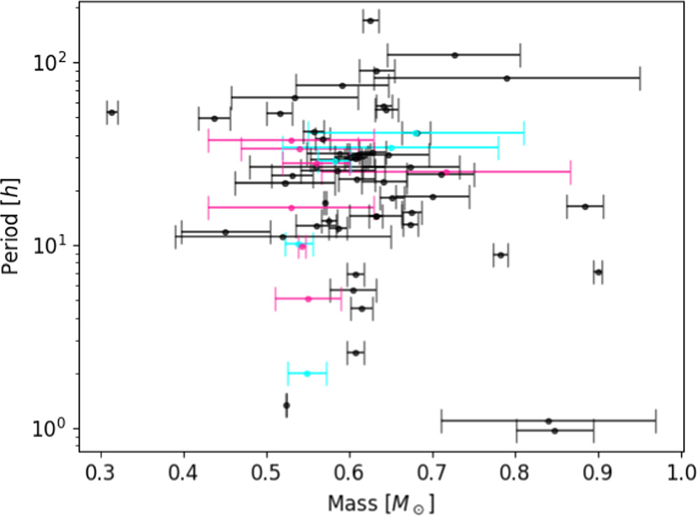
Figure 1. Rotation period vs. mass relation for period determinations from asteroseismology. The period axis is in log scale. The black, cyan, and pink dots indicate DAV, DBV, and DOV stars, respectively.
Download figure:
Standard image High-resolution imageTable 4. WDs with Rotation Periods Determined Previously by Asteroseismology
| Star | Pseism | Type | Mass | References | Star | Pseism | Type | Mass | References |
|---|---|---|---|---|---|---|---|---|---|
| (hr) | (M⊙) | (hr) | (M⊙) | ||||||
| TIC 7675859 | 7.15 | DAV | 0.900 ± 0.005 | (0) | TIC 55650407 | 13.56 | DAV | 0.576 ± 0.009 | (0) |
| TIC 79353860 | 17.06 | DAV | 0.571 ± 0.002 | (0) | TIC 149863849 | 18.07 | DAV | 0.652 ± 0.015 | (0) |
| TIC 201860926 | 8.64 | DAV | 0.548 ± 0.021 | (0) | TIC 343296348 | 12.35 | DAV | 0.587 ± 0.011 | (0) |
| TIC 353727306 | 4.51 | DAV | 0.615 ± 0.013 | (0) | TIC 800126377 | 15.1 | DAV | 0.675 ± 0.012 | (0) |
| TIC 1102242692 | 24.14 | DAV | 0.531 ± 0.025 | (0) | TIC 394015496 | 29.76 | DAV | 0.607 ± 0.013 | (1) |
| TIC 21187072 | 53.76 | DAV | 0.3138 ± 0.0068 | (1) | PG 1159-035 | 33.6 | DOV | 0.54 ± 0.07 | (2) |
| RX J2117.1+3412 | 25 | DOV | 0.716 ± 0.150 | (3) | EPIC 228782059 | 34.1 | DBV | 0.65 ± 0.13 | (4) |
| GD133 | 168 | DAV | 0.6257 ± 0.0098 | (5) | EPIC220274129 | 12.7 | DAV | 0.560 ± 0.024 | (6) |
| PG 0112+104 | 10.2 | DBV | 0.539 ± 0.017 | (7) | EPIC220347759 | 31.7 | DAV | 0.589 ± 0.040 | (8) |
| KIC 4552982 | 18.4 | DAV | 0.700 ± 0.044 | (8) | KIC 4357037 | 22 | DAV | 0.522 ± 0.060 | (8) |
| KIC 7594781 | 26.8 | DAV | 0.674 ± 0.058 | (8) | KIC 10132702 | 11.2 | DAV | 0.52 ± 0.13 | (8) |
| GD 1212 | 6.9 | DAV | 0.608 ± 0.010 | (8) | EPIC201719578 | 26.8 | DAV | 0.561 ± 0.082 | (8) |
| EPIC201730811 | 2.6 | DAV | 0.608 ± 0.010 | (8) | EPIC201802933 | 31.3 | DAV | 0.648 ± 0.048 | (8) |
| EPIC210397465 | 49.1 | DAV | 0.437 ± 0.019 | (8) | EPIC211596649 | 81.8 | DAV | 0.79 ± 0.16 | (8) |
| EPIC211629697 | 64 | DAV | 0.534 ± 0.076 | (8) | EPIC211914185 | 1.1 | DAV | 0.84 ± 0.13 | (8) |
| EPIC211926430 | 25.4 | DAV | 0.586 ± 0.045 | (8) | EPIC228682478 | 109.1 | DAV | 0.726 ± 0.080 | (8) |
| EPIC229227292 | 29.4 | DAV | 0.584 ± 0.031 | (8) | EPIC220204626 | 24.3 | DAV | 0.71 ± 0.04 | (8) |
| EPIC220258806 | 30 | DAV | 0.602 ± 0.020 | (8) | EPIC201806008 | 31.3 | DAV | 0.611 ± 0.014 | (8) |
| KUV02464+3239 | 90.7 | DAV | 0.633 ± 0.021 | (9) | SDSS J0349-0059 | 9.8 | DOV | 0.543 ± 0.004 | (10) |
| Ross 548 | 37.8 | DAV | 0.568 ± 0.009 | (11) | GD 165 | 57.3 | DAV | 0.642 ± 0.010 | (11) |
| WD 1711+657 | 16.4 | DAV | 0.884 ± 0.022 | (12) | PG1707+427 | 16 | DOV | 0.53 ± 0.10 | (12) |
| G29-38 | 32 | DAV | 0.628 ± 0.016 | (12) | GD 358 | 29 | DBV | 0.582 ± 0.020 | (12) |
| EC14012–1446 | 14.4 | DAV | 0.632 ± 0.031 | (12) | EC20058-5234 | 2 | DBV | 0.549 ± 0.024 | (12) |
| KIC 11911480 | 74.7 | DAV | 0.592 ± 0.056 | (13) | SDSS J1612+830 | 0.96 | DAV | 0.848 ± 0.047 | (14) |
| WD 0937+010 | 11.8 | DAV | 0.451 ± 0.053 | (14) | KUV11370+4222 | 5.7 | DAV | 0.605 ± 0.028 | (15) |
| HS 0507+0434B | 40.9 | DAV | 0.681 ± 0.017 | (16) | GD 154 | 55.2 | DAV | 0.645 ± 0.014 | (16) |
| KIC 8626021 | 40.8 | DBV | 0.68 ± 0.13 | (17) | PG 0122+200 | 37.2 | DOV | 0.53 ± 0.10 | (18) |
| HL Tau 76 | 52.8 | DAV | 0.516 ± 0.015 | (19) | G185-32 | 14.5 | DAV | 0.6320 ± 0.0086 | (20) |
| L19-2 | 13.0 | DAV | 0.6742 ± 0.0088 | (21) | LP 133-144 | 41.8 | DAV | 0.557 ± 0.012 | (22) |
| NGC 1501 | 28.1 | DOV | 0.56 ± 0.04 | (23) | G226-29 | 8.9 | DAV | 0.7829 ± 0.0091 | (24) |
| PG 2131+066 | 5.1 | DOV | 0.55 ± 0.04 | (25) | |||||
References: (0) Romero et al. (2024); (1) Romero et al. (2022); (2) Oliveira da Rosa et al. (2022); (3) Córsico et al. (2021); (4) Duan et al. (2021); (5) Fu et al. (2019); (6) Bell et al. (2017); (7) Hermes et al. (2017a); (8) Hermes et al. (2017b); (9) Li et al. (2017); (10) Calcaferro et al. (2016); (11) Giammichele et al. (2016); (12) Kawaler (2015); (13) Greiss et al. (2014); (14) Castanheira et al. (2013); (15) Su et al. (2013); (16) Fu et al. (2012); (17) Østensen et al. (2011); (18) Fu et al. (2007); (19) Dolez et al. (2006); (20) Pech & Vauclair (2006); (21) Bradley (2001); (22) Pfeiffer et al. (1996); (23) Bond et al. (1996); (24) Kepler et al. (1995); (25) Kawaler et al. (1995).
Download table as: ASCIITypeset image
4. Results
Assuming that any inhomogeneity on the stellar surface will manifest itself as variability with the rotation period of the surface, we attribute the variability periods detected for the likely single WDs to rotation. This consideration follows the exclusion of all periods potentially caused by pulsation. On the other hand, the periods detected for the WDs with close pairs and the potential WDs with pairs can represent rotational periods, orbital periods, or even both, in case of synchronization.
Before we present our results, Figures 2 and 3 present examples of time-series analysis for two WDs for which we have detected a variability period. For both figures, the top panel shows the FT, with a red dashed line indicating FAP = 1/1000, and the bottom panel shows the folded light curve for the highest period detected in the FT.
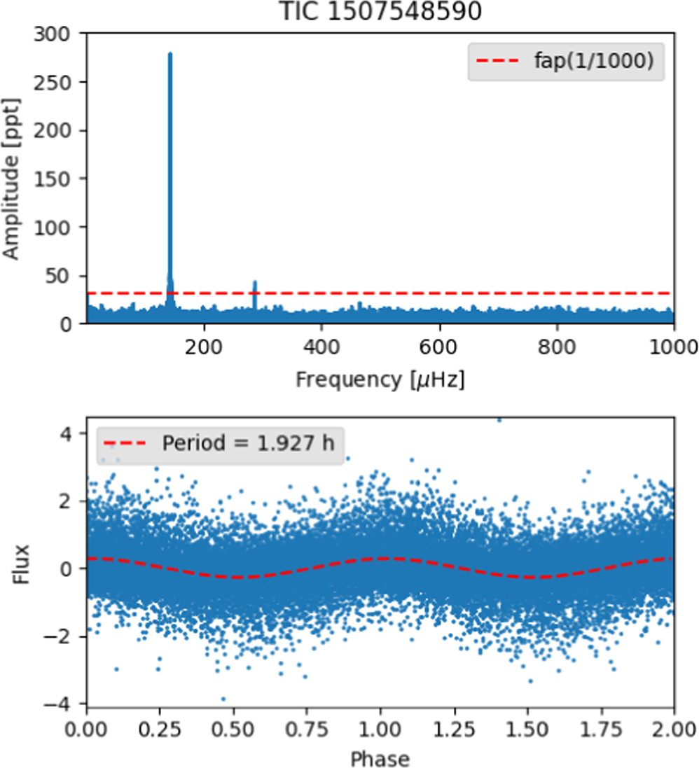
Figure 2. Time-series analysis for the star TIC 1507548590. The top panel shows the FT as well as its FAP of 1/1000 (red dashed line). The bottom panel shows the light curve folded on the period of 1.92772 hr and a sinusoidal curve with the same period in red.
Download figure:
Standard image High-resolution imageFigure 2 shows the Gaia WD candidate TIC 1507548590 (SDSS J 175909.01 + 231155.7) that we classified as a potential WD with pair. It shows Teff = 25,089 ± 2950 K and  cm s−2 (Gentile Fusillo et al. 2021). This is a low-mass (0.214 M⊙) and faint WD, with magnitude G = 17.505—our selected faintness limit. The FT presents two significant peaks: a frequency corresponding to 1.92772 hr and its harmonic. The folded light curve confirms that this is the period corresponding to the main variability of the star.
Figure 3 shows the DA TIC 1100582330 (SDSS J 154119.84 + 120914.6). Its spectra fit Teff = 26,828 ± 107 K and  cm s−2 (Kepler et al. 2015), corresponding to a mass of 0.496 M⊙; it is also faint, at magnitude G = 17.032. The FT presents only one significant peak, with a period of 2.736 hr. This is one of the few stars in our sample of likely single WDs for which it is possible to observe the variability in the folded light curve.
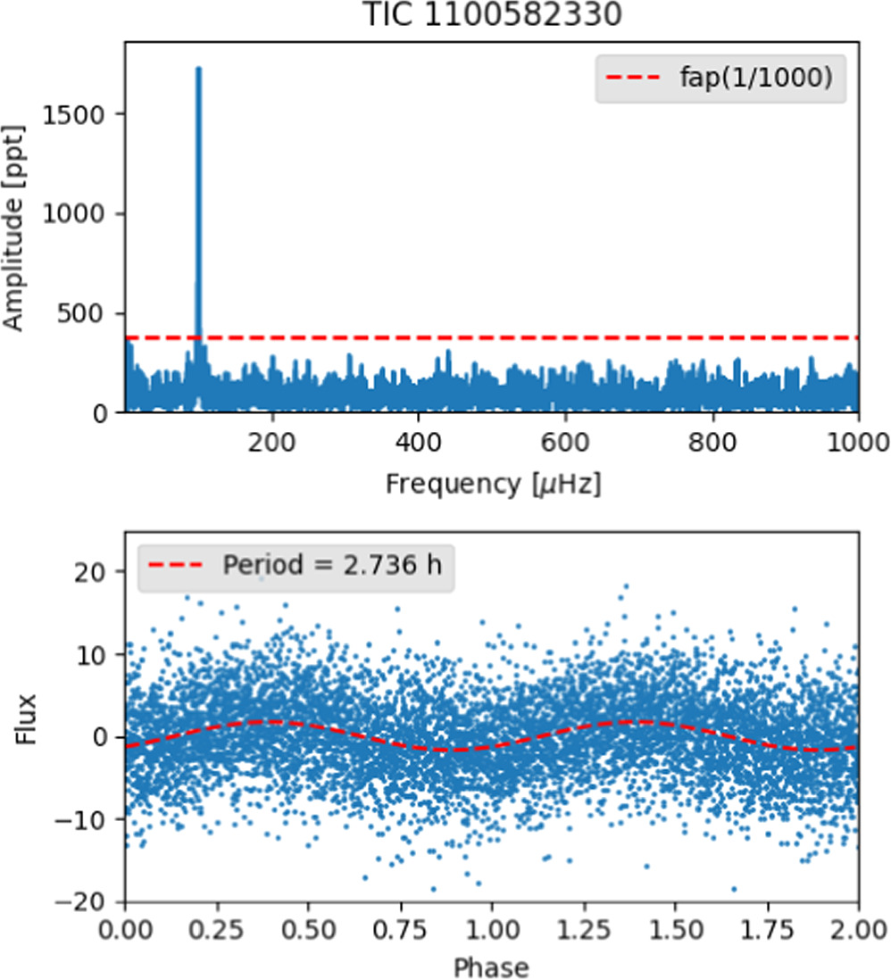
Figure 3. Time-series analysis for the star TIC 1100582330. The top panel shows its FT as well as its FAP of 1/1000 (red dashed line). The bottom panel shows the light curve folded on the period of 2.736 hr and a sinusoidal curve with the same period in red.
Download figure:
Standard image High-resolution image4.1. Mass and Temperature Distribution
Figures 4 (5) show the dependence of the detected period—on a logarithmic scale—on the effective temperature (stellar mass) in the left panel and the effective temperature (mass) distribution in the right panel. The red points and bins denote magnetic WDs, whereas the blue points and bins correspond to WDs with close pairs. It is important to point out that the blue and red bins are independent distributions; their overlap does not correspond to a sample of WDs with both close pairs and magnetic fields detected.
Figure 4 shows that our sample of WDs is distributed around approximately 12,000 K, a representative value of the DA population, which comprises about 80% of the WDs spectroscopically identified (e.g., Kepler et al. 2021). The left panel of Figure 4 shows that there does not appear to be a dependence of the detected periods on the effective temperature. Moreover, the close binaries exhibit a mean temperature of 26,300 K, similar to the complete sample, whose mean temperature is 27,700 K. On the other hand, magnetic WDs present a trend toward low temperatures, with a mean effective temperature of 17,100 K.
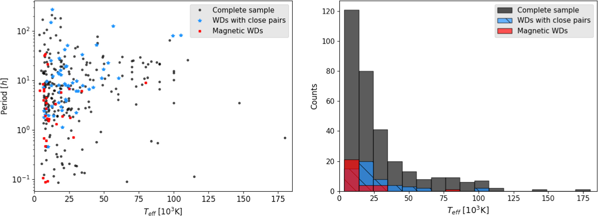
Figure 4. The left panel displays the rotational period in hours vs. the effective temperature in kelvins, both in log scale. The right panel shows the temperature distribution of sample 1. The red and blue dots/bins represent the WDs with magnetic fields and with close pairs detected, respectively.
Download figure:
Standard image High-resolution imageThe left panel of Figure 5 shows that there is no strong dependence of the detected periods on the stellar mass for the complete sample. However, this plot reveals a negative correlation for the likely single WDs, suggesting a trend to shorter rotational periods for more massive WDs. Moreover, we can also observe a positive correlation between period and mass for the WDs with close pairs.
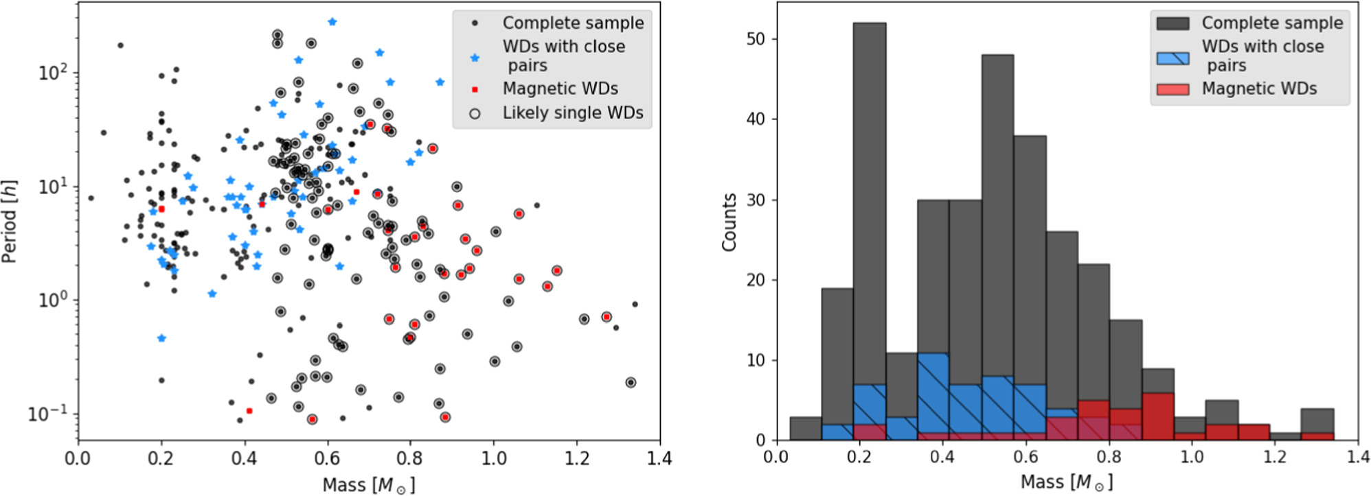
Figure 5. The left panel displays the rotational period in hours in log scale vs. mass in solar masses, while the right panel shows the mass distribution of sample 1. The red and blue dots/bins represent the WDs with magnetic fields and with close pairs detected, respectively. The black circles indicate the stars that comprise the likely single WDs.
Download figure:
Standard image High-resolution imageThe left panel of Figure 5 also shows that most magnetic WDs in our sample exhibit periods shorter than 10 hr and that they are among the targets with the shortest periods. It is essential to recognize that our sample has a selection effect. According to Brinkworth et al. (2013), the rotational period of magnetic WDs exhibits a bimodal distribution, with one group showing periods on the order of minutes to hours and the other displaying periods much longer than their 4 yr of observations. However, their total sample consists of only 26 stars, which is smaller than our sample of 30 magnetic WDs. Each observation cycle (sector) of the TESS telescope lasts ≈27 days, with an interruption of data transfer in the middle, limiting the detection of periods to a few hundred hours. In this way, we detect only the fastest portion of magnetic WDs. Furthermore, massive WDs are fainter and tend to rotate more rapidly (e.g., Hermes et al. 2017b; Caiazzo et al. 2021; Williams et al. 2022). Although TESS is a small telescope, in fact, most of our magnetic sample consists of massive WDs rotating with periods shorter than 10 hr.
The histogram in Figure 5 shows that the mass distribution exhibits two peaks—one sharp peak centered on 0.2 M⊙ and a broader distribution around approximately 0.55 M⊙. The distribution around 0.55 M⊙ is consistent with the values expected for the mass distribution of WDs (e.g., O’Brien et al. 2023). On the other hand, the distribution around 0.2 M⊙, which contains 16% of the sample, cannot be explained by the evolution of single stars.
We included in this work all WDs that the TESS telescope was able to observe with sufficient signal-to-noise ratio (S/N)—mostly WDs with apparent magnitudes lower than approximately 17.5. Therefore, our sample is limited by magnitude rather than volume. As the mass of WDs is inversely proportional to their radius and the brightness of a star is proportional to its radius, the brighter the WD, the less massive it is. This leads to magnitude-limited samples of WDs being biased toward low-mass stars.
To overcome this bias, we corrected the mass distribution of our sample using the method of Schmidt (1968; see, e.g., Liebert et al. 2005; Kepler et al. 2007). In this method, the contribution of each star is weighted by  , where Vmax is the volume defined by the maximum distance at which the star would still be visible. To correct for the nonuniform distribution of stars in our Galaxy, we assumed a Galactic disk scale height of 250 pc, following Fleming et al. (1986) and Liebert et al. (2005). We applied this method using the parallax, apparent magnitude, and galactic latitude from Gaia DR3 (Gaia Collaboration et al. 2018). A Gaia parallax was not available for only one star, which was not included in Figure 6.
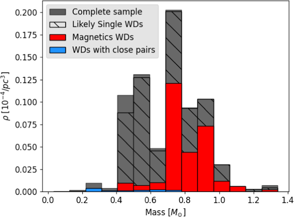
Figure 6. Mass distribution for our complete sample corrected by the  volume. The red and blue bins represent the WDs with magnetic fields and with close pairs, respectively. The hatch-filled bins indicated the likely single WDs.
Download figure:
Standard image High-resolution imageFigure 6 exhibits the mass distribution of our sample corrected by the  volume. It shows that the distribution of low-mass WDs around 0.2 M⊙ has disappeared, confirming that the excess of brighter low-mass WDs in our sample is an observational bias. Furthermore, the distribution also indicates a lack of WDs with approximately 0.6 M⊙, which was supposed to be the most common mass for WD stars. Instead, there is an excess of massive WDs in our sample. Furthermore, it shows that the density of our complete sample is dominated by the likely single WDs sample and that the magnetic WDs of our sample dominate the density of the massive WDs. These results could indicate that our likely single WDs sample is dominated by magnetic WDs resulting from binary interactions (e.g., Toonen et al. 2017; Kilic et al. 2023).
It is relevant to point out that our initial sample of 854 WDs does not present this lack of 0.6 M⊙ stars (see Appendix B). Instead, it exhibits a mass distribution corrected by  , as expected for WDs: centered around 0.6. M⊙ (e.g., Kepler et al. 2021; O’Brien et al. 2023). Therefore, this gap only appears after the high-quality TESS_localize selection.
As already explained in Section 1, some inhomogeneity at the stellar surface of single WDs must be present for us to be able to detect their rotational rates through photometry. The most common way of generating inhomogeneities is by magnetic fields (e.g., Mathys et al. 2024). The origin of the WD magnetic fields is still an open question; however, it is well known that interactions can result in WDs with strong magnetic fields (Tout et al. 2008). One possibility is that the TESS_localize high-quality parameters may have selected targets with higher amplitude variability and, consequently, those with higher magnetic fields. One piece of evidence is that the TESS_localize criteria reduced our initial sample by 56%; however, it reduced only by 11.8% our initial sample of 34 known magnetic WDs.
4.2. Variability Period Distributions
Figure 7 shows the histograms of periods up to 100 hr (right) and up to 30 hr (left) for each sample listed in Table 3. Each line of this figure displays the histograms of one sample, indicated by their legends. The last line of Figure 7 shows the same histograms but for the rotational periods determined by asteroseismology, which are listed in Table 4. The red bins represent the magnetic WDs in each sample.
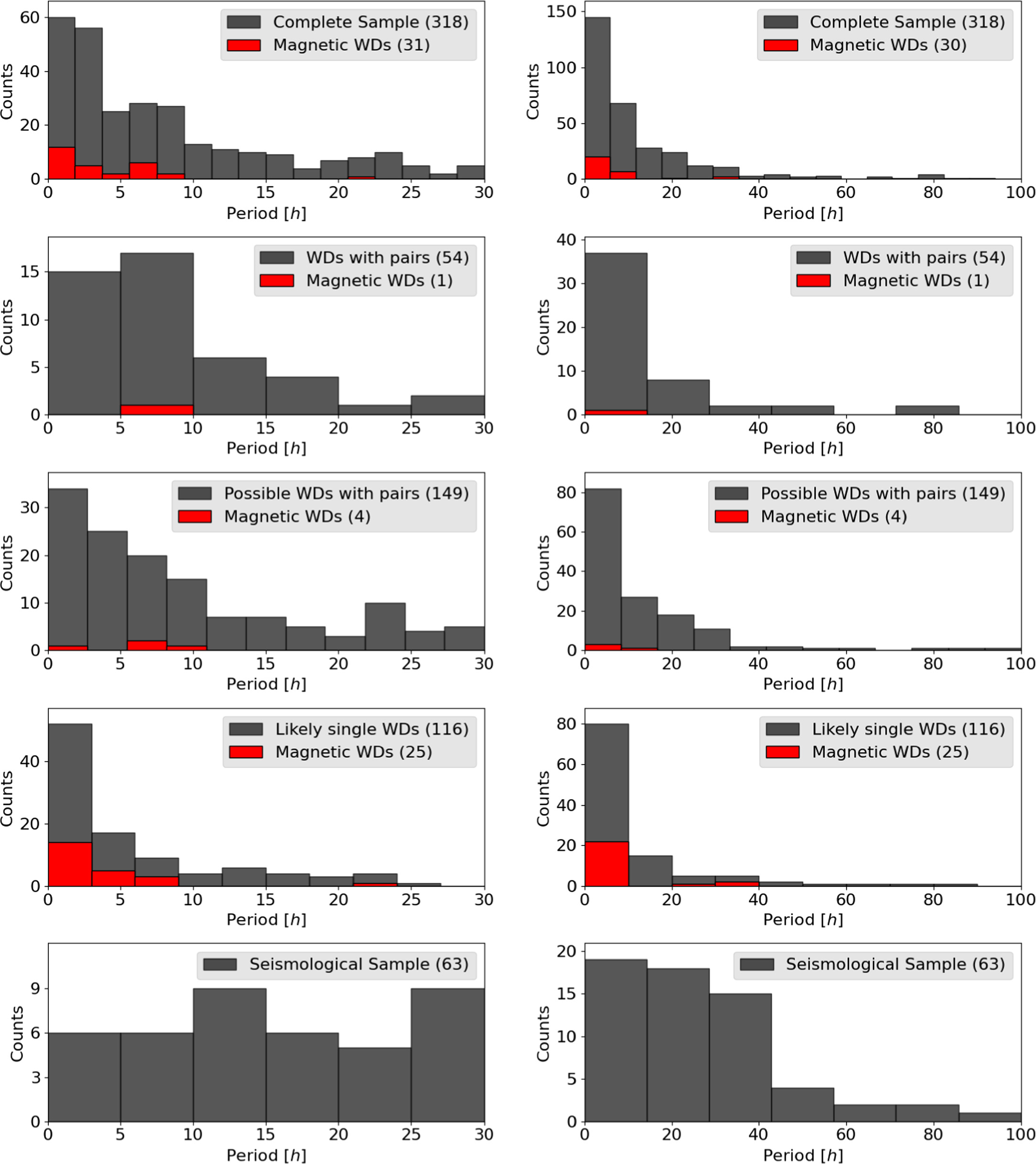
Figure 7. Variability period histograms for different samples of this work and, in the last line, histograms of rotation periods from seismology. On the left, we present the histograms of periods up to 30 hr, and on the right, the histograms of periods up to 100 hr. The red bins show the magnetic population in our samples of WDs. The labels indicate the samples plotted as well as their number.
Download figure:
Standard image High-resolution imageIn the first line of Figure 7 we observe the distribution of our complete sample with its population of 30 magnetic WDs indicated by red bins. The right panel shows that the variability periods are mostly concentrated in the shortest bins. Even considering only periods shorter than 30 hr (left panel) the two shortest bins encompass 36% of our sample. Moreover, this plot shows that our sample of magnetic WDs is concentrated in the shortest periods, presenting a median period of 3.4 hr.
The second line of Figure 7 shows the period histograms for the sample of WDs with close pairs. This sample is composed of 54 stars, one of them with a detected magnetic field. The periods detected for this sample have a median of 8.1 hr. The third line of Section 4.4 illustrates the period distributions for the sample of potential WDs with pairs. This sample is composed of 149 WDs, including four with magnetic fields detected. Their median period is 7.6 hr, close to the median period of the WDs with close pairs.
Finally, the fourth line of Section 4.4 shows the period distribution of the likely single WDs sample. This sample is composed of 115 stars, 25 of them with magnetic fields detected. The right panel shows that the photometric rotation periods are very concentrated in the shortest-period bin, with 69% of periods being shorter than 10 hr. The likely single WDs exhibit a median period of 3.9 hr, very close to the median period exhibited by our complete magnetic sample (3.4 hr). The 25 magnetic WDs included in the likely single WDs sample present an even shorter median period of 1.9 hr.
The last line of Figure 4.4 displays the distribution of the rotational periods estimated through asteroseismology, compiled in Table 4. Despite the difference in sample sizes, this figure shows significant disparities between the rotational distributions derived from photometry and seismology. The seismological sample has a median rotational period of 24.2 hr, which is over 6 times longer than the photometric rotational median period. Additionally, the distribution of rotational periods derived from seismology is broader compared to photometry, with the seismological and the photometric samples exhibiting a MAD of 13.9 hr and 3.5 hr, respectively.
It is important to acknowledge that the rotation period calculated through asteroseismological models is an estimate of the mean internal rotational period of the star; while the photometric rotational period represents the rotation of the stellar surface. Moreover, the seismological sample and the likely single WDs sample are representative of different populations. The seismological sample is representative of the pulsating WDs, whose instability strips are very narrow in temperature range. In contrast, our likely single WDs sample is representative of the WDs with surface inhomogeneities, probably mostly caused by magnetic fields.
As explained in Section 2, we excluded pulsation periods. However, to eliminate any doubts about the short periods in our likely single WDs sample, Figure 8 shows the histogram of periods longer than 0.3 hr. It is important to note that previous work has already detected periods shorter than 0.3 hr for massive WDs (e.g., Barstow et al. 1995; Caiazzo et al. 2021). The inset plot confirms that even with a conservative approach of excluding periods shorter than 0.3 hr, the majority of our sample still exhibit rotation periods shorter than 10 hr.
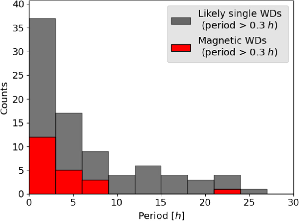
Figure 8. Rotational period distribution up to 30 hr for the likely single WDs excluding periods shorter than 0.3 hr. The red bins indicate the magnetic stars of the sample.
Download figure:
Standard image High-resolution image4.3. Comparison with Ground-based Observations
Moss et al. (2023) obtained time-resolved spectroscopy for two magnetic WDs in our sample at the Gemini Observatory. Based on the shifting positions of the Zeeman-split Hα components, they inferred a rotation period of 0.648 hr for the star TIC 392797216 (LHS 2273). This star is included in our sample of likely single WDs, and the period reported is very close to the 0.68 hr period we found in the TESS data. Using the same method, they found that the star TIC 262548040 (LHS 1243) has a rotation period of 0.216 hr. Due to its low mass of 0.41 M⊙, we classified this star as a possible WD with pair. Figure 9 presents the FT of the data obtained by TESS for this star, showing that only one peak at 2617 μHz (0.106 hr) is above the detection limit (horizontal dashed red line). The vertical dotted lines indicate the peak of 0.106 hr and its double (0.212 hr), showing that there is no significant peak at 0.212 hr in the TESS data. Therefore, this shows that, in this case, the signal we detect in the TESS data is the harmonic of the real rotation period. Despite the harmonic issue, Moss et al. (2023) confirm the rotation rates for two of the fastest rotators in our sample.
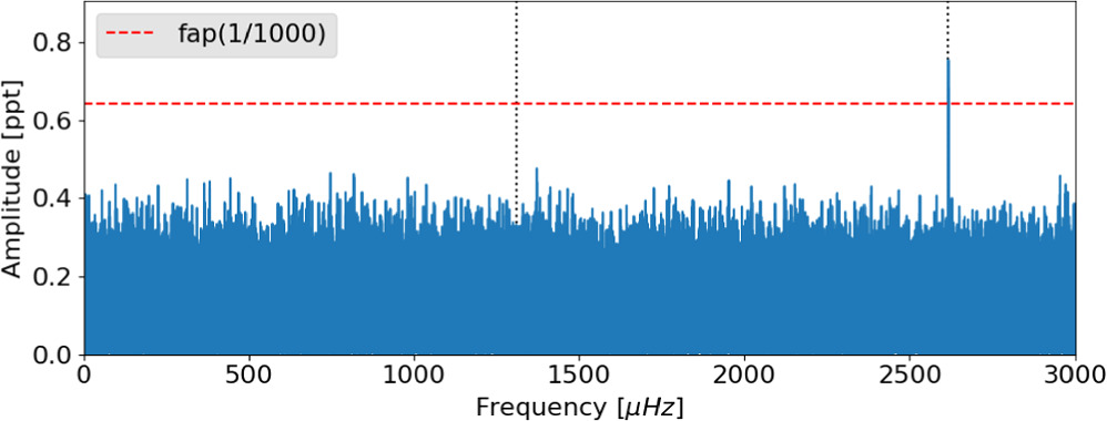
Figure 9. FT of TESS data of star TIC 262548040. The horizontal red line indicates FAP = 1/1000 and the vertical dotted lines indicate the peak of 0.106 hr and its double.
Download figure:
Standard image High-resolution image4.4. Pulsating WDs
From the 61 stars listed in Table 4, 45 were observed by TESS. We analyzed all of them, searching for nonpulsating periods. Most pulsating WDs do not show any frequency with amplitude above the detection limit, other than pulsation periods, or show only low amplitude at frequencies smaller than 4.6 μHz (10 times the frequency resolution of a sector) in the FT. Some pulsating WDs exhibit dozens of pulsation frequencies in their FTs, leading to linear combinations at low frequencies. We only identified reliable variability periods outside the pulsation range (periods longer than 1500 s) for three of these stars: NGC 1501, TIC 7675859, and G226-29. Their TESS_localize output parameters are compiled in Table 2 and are described in the following sections: 4.4.1, 4.4.2, and 4.4.3.
4.4.1. NGC 1501
The pulsating pre-WD NGC 1501 was discovered to pulsate with periods from 5235 s to 1154 s, by Bond et al. (1996). They estimate a rotation period of 1.17 days from a mean splitting of 9.9 μHz. This star was observed by TESS during Sector 19 for 25 days with 120 s exposures. We analyze its FT and detect three variability frequencies outside its pulsating frequency range. TESS_localize confirmed that the source of these signals is NGC 1501. Figure 10 shows this FT up to 200 μHz, where the three nonpulsating frequencies that we have detected are indicated by the vertical dotted lines and correspond to 4.11, 39, and 138 hr. None of these periods is consistent with the rotation period estimated by Bond et al. (1996). Moreover, NGC 1501 is a planetary nebula covered by an ionized gas disk. Therefore, considering the complexity of this system, we are unable to interpret these periods.
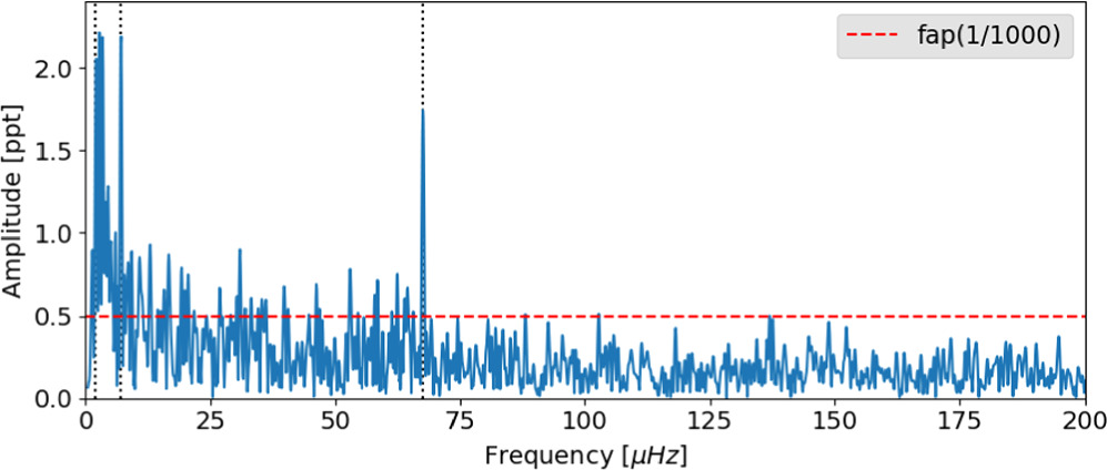
Figure 10. FT of NGC 1501 data at low frequencies.
Download figure:
Standard image High-resolution image4.4.2. TIC 7675859
Romero et al. (2024) determined the asteroseismological rotation period of 7.15 hr for the DAV TIC 7675859 based on data from Sectors 25, 26, 40, 52, 53, and 54. We observed the three components of a high-amplitude triplet in the data of Sectors 52–54 (see Figure 11). The triplet at 1738 μHz is perfectly symmetric, with a frequency spacing Δν = 22.47 μHz. Moreover, we also observed a significant peak at 22.44 μHz (corresponding to 12.3 hr), which is a very close value to the mean frequency spacing of this triplet. The peak at 22.44 μHz is higher than all components of the triplet at 1738 μHz, but we cannot eliminate the possibility that it is a linear combination (Kurtz et al. 2015). This peak of 12.3 hr can also be a subharmonic of the real rotation rate or even the real rotation rate of the stellar surface itself, indicating differential rotation.
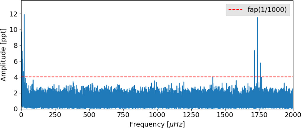
Figure 11. FT of TIC 7675859 data from sectors 52 to 54.
Download figure:
Standard image High-resolution image4.4.3. G226-29
G226-29 is the brightest known DAV, with a known pulsation triplet around 109 s (Kepler et al. 1983). When studying this triplet, Kepler et al. (1995) estimated the rotation period of the WD as 8.9 hr. G226-29 was observed by TESS with 120 s exposures from Sector 14 to 26, and with 20 s exposures from Sectors 40 to 41 and 47 to 60. In total, it was observed along 29 sectors. Data from all sectors show an S/N ≥4.1 wandering peak from 0.93 hr (297.3 μHz) to 3.25 hr (85.5 μHz). As an example, Figure 12 plots the running FT of Sector 51 data. This figure shows the known stable triplet around ∼9200 μHz and a peak that wanders from ∼145 μHz to ∼168 μHz. Figure 13 shows the complete FT of all 20 s data combined, where the wandering peak appears as a broad band at low frequencies (see the inset plot).
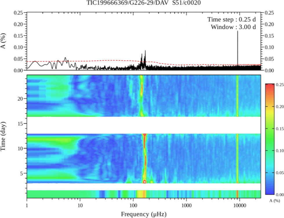
Figure 12. Running FT of G226-29 20 s data from Sector 51. The tall peak on the right is the pulsation triplet around 109 s, while the region around 200 μHz corresponds to the peaks around 4500 s.
Download figure:
Standard image High-resolution image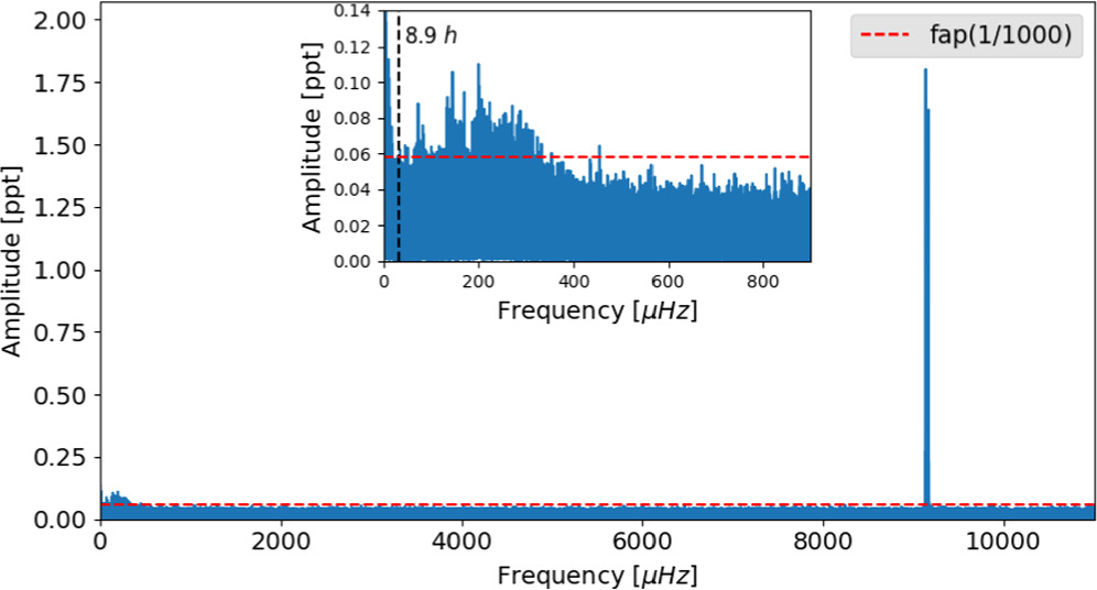
Figure 13. FT of the 20 s data for G226-29 from Sectors 40 to 41 and 47 to 60. The inset plot zooms into the FT at low frequencies. The red dashed line indicates the FAP. The large peak on the right is the pulsation triplet at 109.47235s@1.81mma, 109.27929s@0.57mma, and 109.08690s@1.62mma, while the region around 200 μHz corresponds to the wandering peak around 4500 s.
Download figure:
Standard image High-resolution imageThe methodology described in Section 2.1 assumes that the variability signals are stable. Therefore, to verify whether this wandering peak comes from G226-29, we had to apply the TESS_localize test differently. For each sector, we obtain the highest peak exhibited in such an FT range and run the TESS_localize code for this period. As detailed in Table 2, TESS_localize confirmed that this wandering peak indeed comes from G226-29; however, this variability remains a mystery.
The rotational period from seismology is indicated by a vertical black dashed line in Figure 13, showing the signal we are detecting is not consistent with the rotation of the stellar interior. On the other hand, this signal is very long to be consistent with pulsations. This leads us to suspect differential rotation; that is, the wandering peak could be a manifestation of the rotation of the stellar surface, which is rotating faster than the interior. Although the star has an upper limit on the magnetic field around 10 kG (Valyavin et al. 2006), subsurface magnetic fields, like those in Section 5.2, are a possibility. Radial differential rotation alone does not explain why this peak varies so much, but an angular differential rotation, like the Sun (see, e.g., Snodgrass & Ulrich 1990; Beck 2000), could.
5. Evolutionary Models
If the rotation periods we detect for the likely single WDs sample are due to surface inhomogeneities caused by magnetic fields, we need to calculate models that generate magnetic fields and reproduce the order of magnitude of the rotation rates we are observing. Bagnulo & Landstreet (2020) and Amorim et al. (2023) show that at least 20% of all WDs are magnetic, and Bagnulo & Landstreet (2022), Castro-Tapia et al. (2024a, 2024b), and Blatman & Ginzburg (2024a, 2024b) show a dynamo induced by phase separation during crystallization cannot be the origin for most magnetic WDs. When we study the rotation rates of evolved WD stars, one question that arises is how the evolution changes the internal velocities and how much of the initial angular momentum is lost during the expressive mass-loss phase of AGB before the WD phase. The models included in this section have internal magnetic fields generated by dynamos caused by the rotation of the star and angular momentum transfer. We calculate their rotation rates, internal and at the photosphere, to compare with the observed ones and observe how they change—or not—with the effective temperature of the star.
5.1. Observational and Modeling Context
Using ground-based photometric observation time series from main-sequence stars spanning late-F to early-M spectral types, Fritzewski et al. (2021) determined 279 rotation periods. They found that the rotation periods range from 0.5 days to 32 days, with trends of slow-rotating FGK stars and fast-rotating K dwarfs. In another recent investigation, Labadie-Bartz et al. (2023) explored the rotational characteristics of chemically peculiar (CP) stars using TESS data. Among their findings, they found that the rotation period distribution of CP stars is centered around 3 days. CP stars are observed within the spectral types from early B to early F. Since all stars with spectral types roughly from A to K will become WDs, both works provide evidence that the rotational period of WD progenitors is of the order of days. We have shown in this work that the median photometric rotation period of WDs is 3.9 hr; therefore, these findings suggest that a robust mechanism of internal angular momentum transfer operates during the evolution of these stars.
The asteroseismology of low- and intermediate-mass stars enabled the measurement of the internal rotation rate of WD progenitors at different evolutionary phases (e.g., Deheuvels et al. 2012, 2014, 2015, 2020; Mosser et al. 2012; Di Mauro et al. 2016, 2018; Gehan et al. 2018; Tayar et al. 2019). These inferred rotation rates have been used to constrain models of angular momentum transfer processes. Eggenberger et al. (2019b) and Moyano et al. (2022) found that the transport of angular momentum must be more efficient in more massive stars during the subgiant and red giant phases, even if the efficiency of the internal transport of angular momentum decreases with the evolution of the star. They suggest that the physical nature of the additional mechanism may be different in subgiant and red giant stars. Eggenberger et al. (2022) find that the core rotation rates of the red giant branch models are nearly insensitive to the initial rotation velocity.
On theoretical grounds, Fuller et al. (2019) deduced a new expression for the Tayler instability that leads to larger magnetic field amplitudes, more efficient angular momentum transport, and smaller shear than predicted by the original Tayler–Spruit dynamo. Eggenberger et al. (2019a) applied the new prescription for subgiant and red giant models and found that it leads to low core rotation rates after the main sequence that are in better global agreement with asteroseismic measurements than those predicted by the original Tayler–Spruit dynamo. However, it fails simultaneously to reproduce the asteroseismic measurements available for subgiant and red giant stars.
den Hartogh et al. (2019) found that the rotational periods of the models with additional viscosity are too large in the WD phase. However, the rotational periods match WD rotation periods of the order of 1 day when they exclude the additional effect during the core-helium-burning phase. Therefore, they proposed that the efficiency of the unknown angular momentum transfer process must decrease during the core-helium-burning phase. Applying the Fuller et al. (2019) formalism, den Hartogh et al. (2020) found that when the dynamo effect is turned off at the end of the core-helium-burning phase, the WD rotation rates decrease to the order of days. They concluded that the Fuller et al. (2019) dynamo formalism cannot be the sole solution to the missing process of angular momentum transport in intermediate-mass stars.
Magnetic fields are present in low-mass stars and, when strong enough, can change the rotation by exerting a torque capable of reducing the differential rotation or even imposing uniform rotation throughout the star. Moyano et al. (2023) showed that the transport of angular momentum in radiative zones during the main sequence of low-mass stars must be efficient. They suggested that the internal magnetic fields are a strong candidate for the missing physical ingredient in stellar interiors. In addition, they point out that at least one efficient process able to neutralize the development of differential rotation in stellar interiors must act during the whole evolution of these stars.
5.2. Our Models
We computed evolutionary sequences using the Modules for Experiments in Stellar Astrophysics (MESA) code (Paxton et al. 2011, 2013, 2015, 2018, 2019; Jermyn et al. 2023), release 22.11.1. Our models have an initial mass of Mi = 1.5 M⊙ (following den Hartogh et al. 2019) and an initial metallicity of Z = 0.02, 0.002, and 0.001. The initial mass was chosen to be above the lower limit of 1.3 M⊙ for the convective core in the main sequence (e.g., Aerts & Tkachenko 2023), leading to a WD with a mass close to the mean mass of most WD stars (e.g., Kepler et al. 2007; O’Brien et al. 2023). The models are computed from the zero-age main sequence (ZAMS) until a WD cooling effective temperature of 8500 K. Our models start with equatorial surface rotation velocities of 10 and 50 km s−1, typical of main-sequence stars with 1 and 2 solar masses. These values are assumed to be the solid-body rotations at the ZAMS, which is a reasonable and common assumption for this type of star (see, e.g., Bouvier et al. 1997; Granada & Haemmerlé 2014; Amard et al. 2019; Deal et al. 2020; Nguyen et al. 2022; Douglas et al. 2024). For further information on the models, see Appendix C.
The mixing of elements and the transport of angular momentum due to rotation are implemented in MESA closely following Heger et al. (2000, 2005). Two efficiency factors must be set to calibrate the diffusion coefficients: the contribution of rotationally induced instabilities to the diffusion coefficient is reduced by the factor fc = 1/30, and the sensitivity of rotationally induced mixing is fμ = 0.05.
We consider the following angular momentum transport mechanisms: dynamical shear instability, Solberg–Hoiland, secular shear instability, Eddington–Sweet circulation, Goldreich–Schubert–Fricke and the Tayler–Spruit dynamo.
The final masses of our models are 0.546 M⊙ for Z = 0.02, 0.577 M⊙ for Z = 0.002, and 0.585 M⊙ for Z = 0.001. This aligns with the expectations that stars with higher metallicity should form less massive CO cores and lose more mass in the AGB phase than stars with the same initial mass but lower metallicity (e.g., Dominguez et al. 1999; Catalán et al. 2008; Romero et al. 2015; Choi et al. 2016). Similar models with initial masses of 2.5 M⊙ reach the WD phase with masses around 0.6 M⊙.
In Figure 14, we show the evolution of the surface rotational period (P) versus the effective temperature (Teff) during the cooling track for a set of model sequences with different metallicity and initial rotation velocity. The surface rotational period is computed via P = 2π r/v, where r is the radius of the model and v is the rotational velocity at the equator. Sequences that consider the six mechanisms of angular momentum transport are shown as dotted lines (AMT = ON), and solid lines represent sequences with all mechanisms turned off (AMT = OFF).
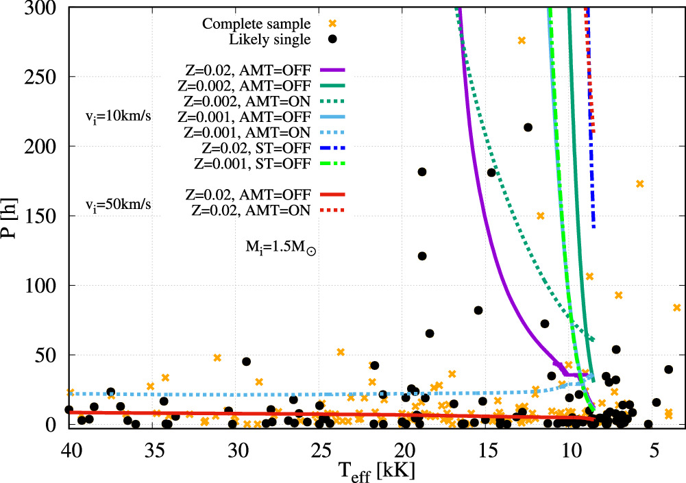
Figure 14. Observational data of the surface rotation of WD stars (orange crosses for the complete sample and black dots for the likely single sample) are compared against evolutionary models showing the rotation period in the WD cooling track. We compare models with the six mechanisms of angular momentum transport turned off (solid lines) and on (dotted lines) during the whole evolution. For an initial rotational velocity of vi = 10 km s−1, we present models with metallicities of Z = 0.02 (purple), 0.002 (dark green), and 0.001 (light blue). We also compare two models where the Tayler–Spruit dynamo is the only mechanism that is turned off during the computations (dark blue and light green dotted–dashed lines). For an initial rotational velocity of vi = 50 km s−1, we compare two models with Z = 0.02 (red lines). All model sequences have an initial mass of 1.5 M⊙.
Download figure:
Standard image High-resolution imageFor vi = 10 km s−1 and Z = 0.02 (the purple line in Figure 14), we find that the WD models with AMT = OFF decrease the average equatorial rotation period on the surface from P = 300 hr to ∼ 30 hr when cooling from ∼ 17 kK to 8500 K. The sequence with AMT = ON does not even reach 300 hr before cooling down to the same temperature (and therefore does not appear in the plot).
For sequences with Z = 0.002 (the dark green lines in Figure 14), we find that if AMT = OFF (solid line), the models brake from P = 300 hr to 40 hr only at the very end of the cooling track (Teff < 10 kK), while the AMT = ON sequence (dotted line) has already spun down to 300 hr when Teff < 17 kK, although it reaches only P ∼ 60 hr at Teff = 8500 K.
The internal redistribution of the angular momentum is very efficient early in the evolution of low-mass stars (e.g., Mosser et al. 2012). This suggests that when AMT = ON, a large amount of mass lost by winds during the AGB phase carries away most of the angular momentum, and thus the surfaces of the models rotate slower in the WD phase.
The difference in turning the angular momentum transport mechanisms on and off is much more pronounced for low metallicity (Z = 0.001; the light blue line in Figure 14). While AMT = OFF (solid line) follows the same trend as for higher metallicities (that is, it only reaches low P at the end of the cooling track), the sequence with AMT = ON (dotted line) cools from Teff = 40 kK down to 8500 K, with an approximately constant rotation period of P = 25 hr, closer to most of the observed period distributions.
In Figure 14, we also show two sequences of models with vi = 10 km s−1, where the Tayler–Spruit mechanism was turned off and all the other five mechanisms were kept on throughout the evolution (ST = OFF; dotted–dashed lines). For Z = 0.001 (the light green line), the result is similar to that for the same metallicity, but with all six angular momentum transport mechanisms turned off. This suggests that the Tayler–Spruit mechanism dominates over the other mechanisms from the point of view of rotation analysis during the WD phase.
Finally, we present two sequences with vi = 50 km s−1 and Z = 0.02. These models show that observational data with a shorter rotation period (P < 50 hr) are better adjusted by models with AMT = OFF, while models with AMT = ON present a rotation period shorter than 300 hr only at the end of WD cooling, when Teff < 10 kK. This suggests that if we disregard the Tayler–Spruit mechanism throughout the evolution, models with a higher initial velocity (50 km s−1) fit the WD rotation data better if the initial mass is 1.5 M⊙.
The dominant factors for the spin-up of the external layers during the WD cooling phases are the He convection zones that arise at Teff ≃ 32,000 K, followed by the H convection zone, if the star has an H envelope, around Teff ≃ 14,000 K. The movement of mass in the convection zones efficiently redistributes the angular momentum.
Also, the models with AMT = ON generate internal magnetic fields due to differential rotation, as shown in Figure 15 for a model sequence with Mi = 1.5 M⊙, Z = 0.001, and vi = 10 km s−1 (corresponding to the dotted light blue line in Figure 14). According to Spruit (2002), the Maxwell stresses transport angular momentum in the radial direction at a rate proportional to the product Br Bϕ . In Figure 15, the x-axis represents the mass coordinate of the model, with the core on the left and the surface on the right, and the y-axis shows the intensity of the magnetic field components Br and Bϕ in the internal part of the models at two different temperatures during the cooling track. The chosen temperatures, 25,000 K and 11,000 K, are representative of the DAV and DBV variable classes.
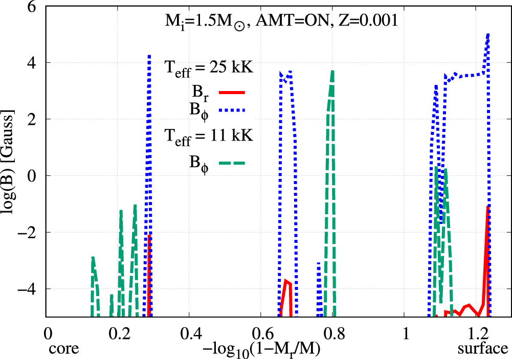
Figure 15. Internal magnetic field at Teff = 25,000 K and 11,000 K, generated by the Tayler–Spruit dynamo during the evolution due to differential rotation caused by angular momentum transfer throughout the stellar evolution. Br is the radial field and Bϕ is the azimuthal one. The properties of the initial model in ZAMS are Mi = 1.5 M⊙, Z = 0.001, and vi = 10 km s−1. For Teff = 25,000 K, the solid red line shows the radial component and the dotted blue line represents the azimuthal one. For Teff = 11,000 K, the dashed green line shows the azimuthal component and the radial component does not have enough intensity to appear in the plot. The six angular momentum transfer mechanisms operate throughout the evolution. Magnetic field values are negligible beyond 1.3 on the x-axis, i.e., toward the surface.
Download figure:
Standard image High-resolution imageFigure 15 shows that during cooling, the azimuthal component of the magnetic field is always greater than the radial component. In some regions, the magnetic field reaches an intensity of ∼104 G. We also found that both components tend to be less intense as the models cool, and the outer ∼5% (by mass) of the models shows no significant magnetic fields.
As a general behavior, the models suggest the following. During cooling, the Tayler–Spruit dynamo mechanism acts smoothly in the core, flattening the rotation profile up to the He layer. On the other hand, a convective zone appears at the base of the He envelope around 32,000 K and increases in size inward as the models cool, causing angular momentum to be transferred from the core and the He zone.
Around 14,000 K, a convective zone develops at the base of the H envelope, and then the rotational speed on the surface is as high as that of the fastest part of the core and the He zone. The exact temperature for this to occur depends on the metallicity and, especially, on the history of mass loss at the end of the AGB phase. This is because the last thermal pulses directly interfere with the amount of H remaining in the model that enters the cooling track, modifying the convection in this zone.
Thus, the internal rotation profile of the models during cooling depends, to some extent, on angular momentum transfer mechanisms, but also strongly depends on convection in the He and H zones.
6. Conclusion
We have reported significant variability periods for 318 WDs, as well as their variability amplitudes and quality criteria. We divided the 318 stars composing the complete sample into three subsamples. 54 of them were classified as WDs with close pairs, and their variability periods can be due to orbital motion or rotation. The other 149 were classified as potential WDs with pairs, due to their low masses and/or high temperatures (e.g., Steen et al. 2024). Finally, we classified 115 as likely single WDs and therefore attributed their variabilities to rotation.
Our 30 magnetic WDs are massive, fast rotators, and cold, while our 54 WDs with close pairs are well distributed on the mass range and present a weak tendency of longer periods to massive WDs.
Our complete sample of 318 WDs exhibits a temperature distribution expected for DA WDs, peaking around Teff ≃ 12,000 K. On the other hand, its mass distribution is biased toward low-mass stars, because it is a magnitude-limited sample. The mass distribution corrected by  presents, in density, a lack of WDs with a mass around 0.6 M⊙ and an excess of massive WDs, which are dominated by our little sample of 30 magnetic WDs. These peculiarities are not present in the corrected mass distribution of our initial sample of 854 stars, which leads us to conclude that these characteristics were introduced by the TESS_localize high-quality selection. In this second selection, 89% of the stars discarded by TESS_localize were done because the software was unable to perform a high-quality fit. Therefore, it is possible that TESS_localize has selected the highest amplitude variabilities and, consequently, the WDs with the strongest magnetic field. This could lead to a mass distribution dominated by magnetic WDs resulting from binary interactions and possibly explain the lack of 0.6 M⊙ WD density.
The stellar density of our sample is completely dominated by the likely single WDs, which, as already discussed, are probably composed of magnetic WDs. A piece of evidence is that TESS_localize reduced our initial sample by 56%; however, it only reduced by 11.8% our initial sample of 34 known magnetic WDs.
The likely single WDs present a median rotational period of 3.9 hr, which is far shorter than the median rotational period from seismology estimates, 24.2 hr. However, this is an expected result, once both estimates of rotation represent different populations. The seismological sample represents the mean internal rotation of pulsating WDs, while our sample of likely single WDs represents the rotation of the stellar surface of WDs with inhomogeneities at their surface.
From the 61 WDs with rotation periods determined by asteroseismology, we detected nonpulsating periods in the TESS data for three of them: NGC 1501, TIC 7675859, and G 226-29. We were not able to interpret with certainty any of these periods. This failure in finding photometric rotational periods for the seismological sample using TESS data reinforces the seismological and likely single WDs samples representing distinct populations. Up to now, we do not know of any pulsating WD with a magnetic field confirmed.
Using ground-based observations, Moss et al. (2023) confirmed the rotation period we detected in the TESS data for two of the fastest rotators in our sample; however, they also provided an example of half-period aliases. This suggests the possibility that we may be detecting and reporting half of the real rotation periods for other stars. On the other hand, this work confirmed rotation periods of 0.68 hr and 0.21 hr for two magnetic WDs in our sample; therefore, it does not invalidate our findings.
For five of the 318 WDs in our sample, all of them included in our sample of likely single WDs, the variabilities detected in the TESS data were also reported by Farihi et al. (2024). They are TIC 328029653, TIC 251080865, TIC 251903434, TIC 204440456, and TIC 321979116. The periods reported agree with our findings. They claim that the variability found in the WD 2138-332 data (TIC 204440456) is the stellar rotation period, almost certainly due to magnetism. In addition, the orbital period of the EMLV TIC 308292831 was already reported by Lopez et al. (2021).
Figure 14 presents two models that at 40 kK reach rotation periods consistent with the observational findings of this work. We find that periods shorter than 50 hr are well fitted by models with Z = 0.02, vi = 50 km s−1, and angular momentum transport set to OFF, or by models with Z = 0.001, vi = 10 km s−1, and angular momentum transport set to ON. A smaller part of the observational data presents a large dispersion of the rotation period and is concentrated at Teff < 20,000 K. Our remaining models best fit these stars.
While other studies have shown that the internal transfer of angular momentum should be intense in the early phase of the evolution of low-mass stars, our study confirms that if we seek to match most of the WD rotational data, this redistribution should cease or be less intense before the end of the AGB phase, when stars lose the highest amount of mass and, therefore, angular momentum. If we assume that stars with lower metallicity will have a lower mass-loss rate due to winds at the top of the AGB phase (e.g., see the discussion in Höfner & Olofsson 2018), this means that they will lose less angular momentum and therefore rotate faster in the WD phase. However, when we consider that more angular momentum transfer mechanisms have been activated since the beginning of the evolution, more angular momentum will be transferred to the surface and lost during the AGB phase. Thus, in terms of the WD rotation period, lowering the metallicity is equivalent to reducing the angular momentum transfer mechanisms in the early evolution. Due to their intrinsic faintness, the observed WDs are mainly nearby galactic disk objects, most likely with metallicity closer to the Sun’s.
In general, our models agree with the most recent results in the literature, in the sense that different initial parameters can be used to create models that are in agreement with a particular part of the observational data, but there is a degeneration in the parameter space (i.e., the initial velocity of rotation, initial mass, metallicity, etc.) that could be better resolved if we knew more precisely how the redistribution of angular momentum occurs in stellar interiors.
In the future, we will analyze the TESS data observed after 2023 October, calculate models with the Fuller dynamo prescription, and extend the mass range of the models, as the data include WDs with a range of masses. We intend to perform spectropolarimetry to check if our likely single WDs are magnetic. We also intend to confirm the rotational periods using high-resolution spectroscopic observations to detect the non-LTE line core rotational broadening, as in Berger et al. (2005).
Acknowledgments
We thank the referee for the valuable comments and suggestions that improved our paper significantly. This work was carried out with the financial support of the Conselho Nacional de Desenvolvimento Científico e Tecnológico (CNPq) and by the Coordenação de Aperfeiçoamento de Pessoal de Nível Superior—Brasil (CAPES). Most of the calculations were performed at the Texas Advanced Computing Center, located at the University of Texas in Austin. We thank Stéphane Charpinet for maintaining the Evolved Compact Stars with TESS on TASOC and for providing the running Fourier Transform of the star G226-29. This research has made extensive use of NASA's Astrophysics Data System Bibliographic Service (ADS), SIMBAD, and MAST. We used ASTROPY (https://www.astropy.org/), TESS-LS (https://github.com/ipelisoli/TESS-LS), TESS_localize (https://github.com/Higgins00/TESS-Localizer), lightkurve (https://docs.lightkurve.org/), and PYRIOD (https://github.com/keatonb/Pyriod).
Appendix A: Known RR Lyrae Star
BPM 24754 (TIC 367227831) is a known variable DAV WD. Figure 16 shows its FT of TESS data plotted using the Pyriod software (Bell 2020). In this case, we know that the primary signal at 21.49 μHz (12.92 hr) and its harmonics are the contamination from the known RR Lyrae variable Gaia DR3 5923100101270979328 (TIC 367227833). The results of the software TESS_localize for the three sectors where the star is observed (12, 39, and 66) are presented in Table 5.
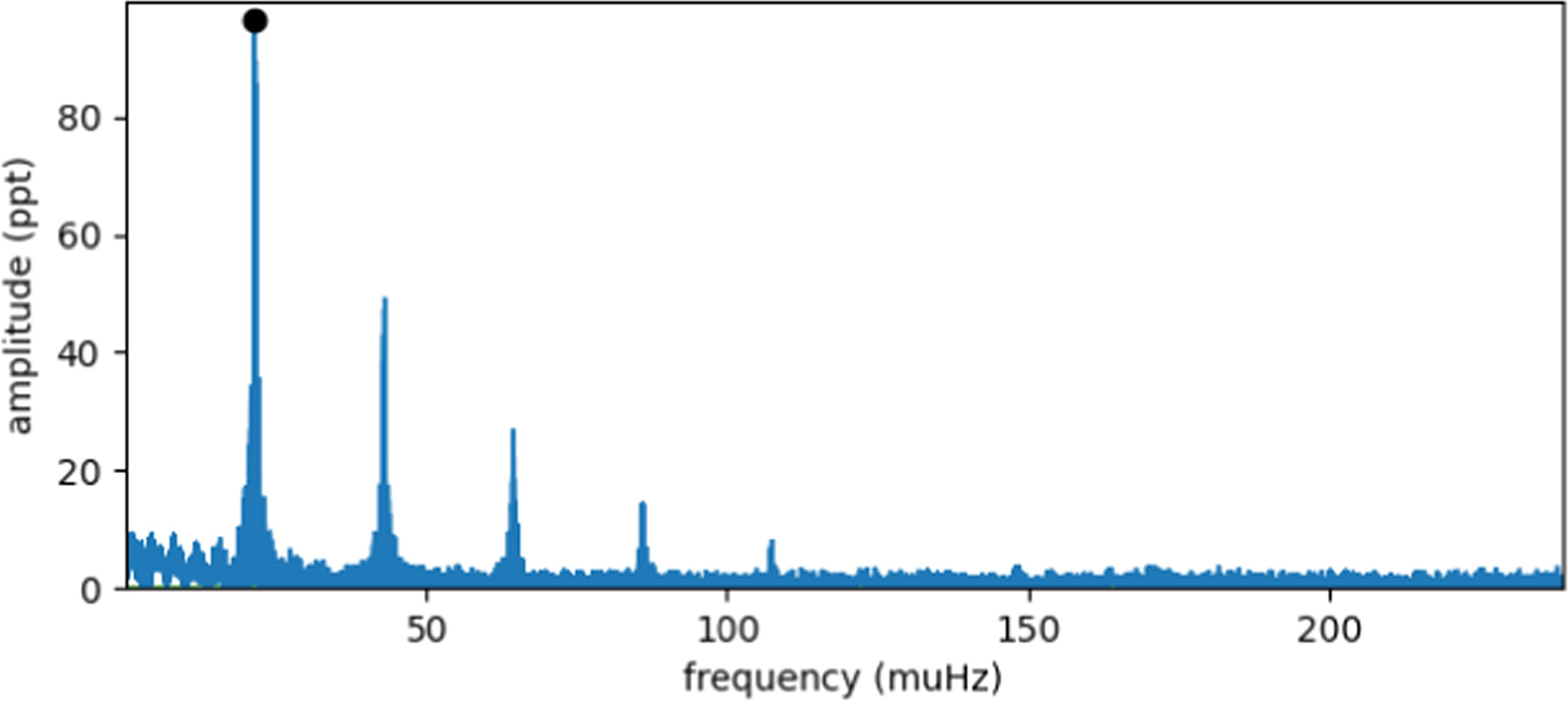
Figure 16. BPM 24754 light curve from Sectors 12, 39, and 66.
Download figure:
Standard image High-resolution imageTable 5. TESS_localize Results for the Signal 12.92 hr Present in the Light Curve of the DAV BPM 24754
| Sector | Source Gaia DR3 | p-value | Relative Likelihood | χ2 | Height |
|---|---|---|---|---|---|
| (σ) | |||||
| 12 | 5923100101270979328 | 0.214 | 0.75 | 44.40 | 42.40 |
| 12 | 5923100101249048320 | 0.071 | 0.19 | 44.40 | 42.40 |
| 39 | 5923100101270979328 | 0.503 | 0.83 | 312.71 | 17.30 |
| 39 | 5923100101249048320 | 0.191 | 0.11 | 312.71 | 17.30 |
| 66 | 5923100101270979328 | 0.829 | 0.96 | 62.47 | 37.22 |
| 66 | 5923100101249048320 | 0.198 | 0.03 | 62.47 | 37.22 |
Download table as: ASCIITypeset image
TESS_localize estimates the probability that the signal source is the RR Lyra star as being 75% in Sector 12, with even the parameters p-value and height indicating good values. The relative likelihood of the RR Lyrae star being the source of the signal increases in the subsequent sectors, with the mean like reaching 85%. The second source is likely the same for all three sectors, Gaia DR3 5923100101249048320. This object is located 306 away from the RR Lyrae star.
Appendix B: Initial Sample of 854 WDs
Our initial sample is composed of 854 WD stars exhibiting a nonpulsating period in their photometric data from TESS for which, at least for one sector, TESS_localize indicates the WD as the most probable signal source. As explained in Section 2.1, most of our initial sample was discarded because TESS_localize was unable to obtain a high-quality fit for the data. That means that for most of the stars in this sample, we are not able to determine with high confidence whether the source of the signal we detected is, in fact, the WD. Figure 17 presents the mass distribution corrected by the  method and the period distribution for our initial sample. The corrected mass distribution is centered around approximately 0.6 M⊙, as expected for WD stars. Magnetic WDs are more massive, exhibiting a distribution around approximately 0.8 M⊙. The period distribution is heavily concentrated in the shortest-period bins, with the sample having a median period of 11.85 hr and a MAD of 11.56 hr.
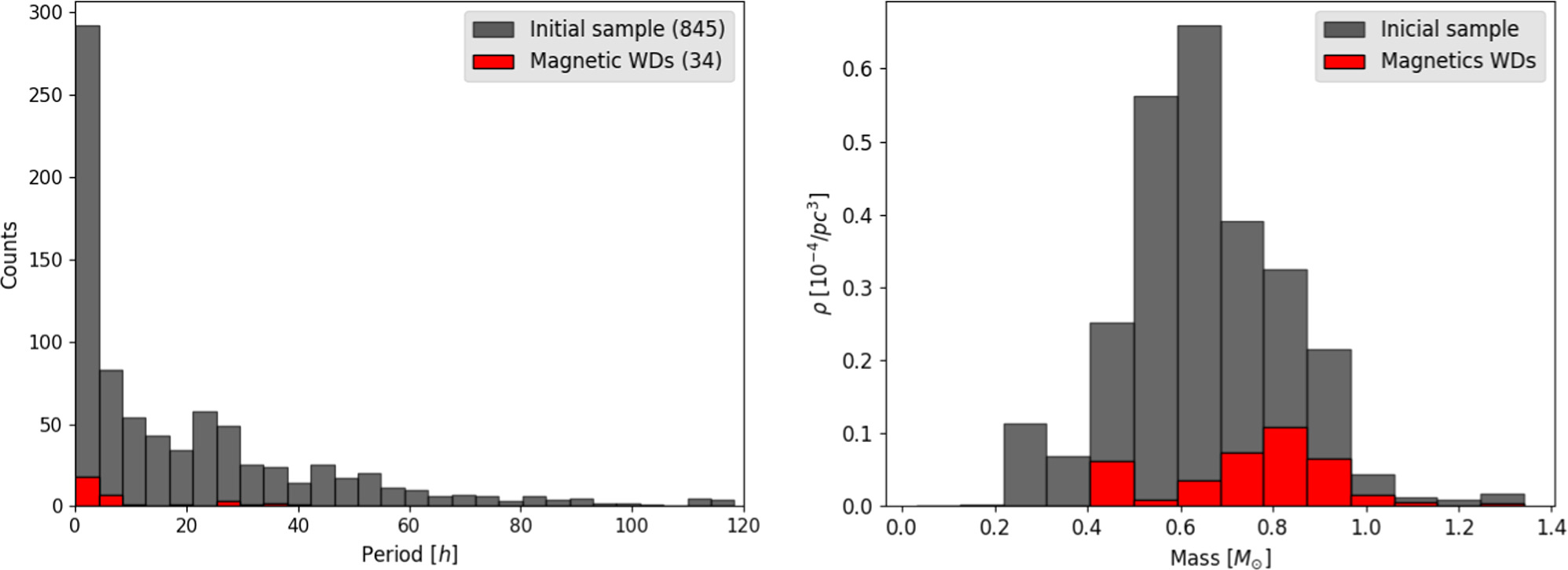
Figure 17. Mass distribution for our initial sample corrected by the  volume.
Download figure:
Standard image High-resolution imageAppendix C: Evolutionary Model Input
Hydrogen and helium burning are computed using the pp_and_cno_extras.net network, which accounts for 25 isotopes and 79 net reactions. Convection is treated using the formulation of the mixing length theory (Böhm-Vitense 1958) in the variation of Henyey et al. (1965), allowing the convective efficiency to vary with the opacity. We set the diffusion of elements for the whole net; each isotope in the network is treated as its own class.
Following the MIST project (Choi et al. 2016), αMLT = 1.82 is adopted as the mixing length parameter. We consider the Ledoux criterion of stability, which considers the influence of composition gradients on mixing. Semiconvection is considered in unstable regions by the Schwarzschild criterion, but in stable ones by Ledoux, with an efficiency parameter αsc = 0.1. Thermohaline mixing is included throughout evolution, with efficiency αth = 666.
Exponential overshooting is set to f = 0.008 in the core and 0.0087 in the shell. We handle the mixing in the convective zones using the convective premixing scheme. For the boundary conditions of the atmosphere, we use the T(τ) Eddington relation with varying opacity for most of the evolution and hydrogen atmosphere tables for cool WDs (Rohrmann et al. 2011), when the models are on the cooling track and the effective temperature is below 10,000 K. The mass loss by stellar winds is taken into account using the Reimers (1975) scheme, with ηR = 0.5 for the red giant branch phase, and the Bloecker (1995) scheme, with ηB varying between 0.1 and 1 for the AGB phase.