Abstract
The circumstellar disk density distributions for a sample of 63 Be southern stars from the BeSOS survey were found by modeling their Hα emission line profiles. These disk densities were used to compute disk masses and disk angular momenta for the sample. Average values for the disk mass are 3.4 × 10⁻⁹ and 9.5 × 10⁻¹⁰ M⋆ for early (B0–B3) and late (B4–B9) spectral types, respectively. We also find that the range of disk angular momentum relative to the star is (150–200)J⋆/M⋆ and (100–150)J⋆/M⋆, again for early- and late-type Be stars, respectively. The distributions of the disk mass and disk angular momentum are different between early- and late-type Be stars at a 1% level of significance. Finally, we construct the disk mass distribution for the BeSOS sample as a function of spectral type and compare it to the predictions of stellar evolutionary models with rapid rotation. The observed disk masses are typically larger than the theoretical predictions, although the observed spread in disk masses is typically large.
1. Introduction
A Be star is defined by Collins (1987) as “a non-supergiant B star whose spectrum has, or had at some time, one or more Balmer lines in emission.” The accepted explanation for the emission lines is the presence of a circumstellar envelope (CE) of gas surrounding the central star, analogous to the first model of a Be star proposed by Struve (1931). The material is expelled from the central star and placed in a thin equatorial disk with Keplerian rotation (Meilland et al. 2007). Different mechanisms such as rapid rotation (Porter 1996; Domiciano de Souza et al. 2003; Townsend et al. 2004; Frémat et al. 2005), mass loss from the stellar wind (Bjorkman & Cassinelli 1993; Stee & de Araujo 1994; Curé 2004; Silaj et al. 2014a), binarity (Okazaki et al. 2002; Romero et al. 2007; Oudmaijer & Parr 2010), magnetic fields (Donati et al. 2001; Cassinelli et al. 2002; Neiner et al. 2003), and stellar pulsations (Rivinius et al. 2003) have been proposed to explain how the star loses enough mass to form the CE and how this material is placed in orbit, but it seems that more than one mechanism is required to reproduce the observations. Such mechanisms must continually supply enough angular momentum from the star to form and to maintain the disk. Given some mechanism to deposit material into the inner edge of the disk, the evolution of the gas seems well described by the viscous disk decretion model presented by Lee et al. (1991), with angular momentum transported throughout the disk by viscosity (Rivinius et al. 2013a).
Be stars are variable on a range of different timescales associated with a variety of phenomena occurring in the disk. For example, short-term variations (∼hours–days) in the emission lines are associated with nonradial pulsations, probably due to the high rotation rate of the central star (e.g., Rivinius et al. 2003, 2013a); intermediate-term variations (∼months–years) are seen in the cyclical variation between the violet and red peaks in doubled-peaked emission lines. Such variations are well represented by the global disk oscillation model (Okazaki 1997; Carciofi et al. 2009). Longer-term variability—in some cases the emission lines disappear and/or are formed again on timescales of years to decades—is associated with the formation and dissipation of the disk (see Section 5.3.1 of Rivinius et al. 2013b, for several examples).
Spectroscopy of the emission lines can be used to get information about the geometry, kinematics, and physical properties of the disk. A very convenient model, in agreement with observations, is to assume that the density in the disk’s equatorial plane falls with a power law with exponent n and follows a Gaussian model in the vertical direction (see details provided in Section 3.1).
We use the density distribution described above, the radiative transfer code BEDISK, and the auxiliary complementary code BERAY to solve the transfer equation along many rays (∼105) through the star/disk configuration. A grid of calculated Hα line profiles from models with different disk density distributions and stellar parameters is used to match the observed Hα line profiles and provide constraints on the disk parameters. We apply this method to a sample of 63 stars from the BeSOS catalog. We selected a fraction of the best-fitting models and obtained the distribution of the disk density parameters, mass and total angular momentum content in the disk, with results provided for both early- and late-type Be stars.
This paper is organized as follows: Our program stars and reduction steps are given in Section 2. Section 3 describes our theoretical models, including the main assumptions of BEDISK and BERAY codes in Section 3.1. Input parameters to create the grid of models are provided in Section 3.2. Section 4 describes our results from selecting best-fit disk density parameters from all our sample stars in two ways: visual inspection (Section 4.2) and a percentage of the best models (Section 4.3). Section 4.4 gives the mass and angular momentum distributions of the disks. A discussion and conclusions of our main results are presented in Sections 5 and 6, respectively. The
2. Sample and Data Reduction
We selected Be stars with B spectral type near or on the main sequence from the Be Stars Observation Survey (BeSOS4 ) catalog for our study. All Be targets on the BeSOS website are confirmed as a Be star in the BeSS5 catalog or have an IR excess in the spectral energy distribution. This gives us a total of 63 Be stars. The sample distribution of spectral type is shown in Figure 1. Approximately 30% of our sample corresponds to the B2V spectral type. The same distribution was found previously by other authors (Slettebak 1982; Porter 1996), with B2V being the most frequently observed spectral type in Be stars.

Figure 1. Histogram of the sample of Be stars by spectral type. The distribution peaks at B2, which corresponds to ∼30% of the sample.
Download figure:
Standard image High-resolution imageBeSOS spectra were obtained using the Pontifica Universidad Catolica (PUC) High Echelle Resolution Optical Spectrograph (PUCHEROS) developed at the Center of Astro-Engineering of PUC (Infante et al. 2010). The instrument is mounted at the ESO 50 cm telescope of the PUC Observatory in Santiago, Chile, and has a spectral range of 390–730 nm with a spectral resolution of λ/Δλ ∼ 18000. Details about the instrument are provided in Vanzi et al. (2012). Observations were acquired between 2012 November and 2015 October. The exposure time was chosen to reach a signal-to-noise ratio (S/N) in the range of 100–200 (as a consequence, the BeSOS catalog has a limiting magnitude of V < 6 in the sample selection criteria). For the wavelength calibration, exposures of ThAr lamps were used. The data reduction was performed using IRAF (Tody 1993) following standard reduction procedures described in “A User’s Guide to Reducing Echelle Spectra with IRAF.”6 The basic steps included removing bias and dark contributions, flat-fielding, order detection and extraction, fitting the dispersion relation, normalization, wavelength calibration, and heliocentric velocity corrections.
3. Theoretical Models
3.1. Disk Density and Temperature Structure
We calculated theoretical Hα line profiles using two codes: BEDISK, a non-local thermodynamic equilibrium (non-LTE) code developed by Sigut & Jones (2007), and BERAY (Sigut 2011), an auxiliary code that uses BEDISK's output to solve the transfer equation along a series of rays (∼105) to produce model spectra.
There are two significant components that must be specified to model the physics of a star+disk system: the density distribution of the gas in the disk and the input energy provided by the photoionizing radiation field of the central star. Assuming both, the BEDISK code solves the statistical equilibrium equations for the ionization states and level populations using a solar chemical composition. Then, the code calculates the temperature distribution in the disk by enforcing radiative equilibrium. All calculations are made under the assumption that the vertical density distribution is fixed in approximate hydrostatic equilibrium, and the geometry of the disk is axisymmetric about the stars’s rotation axis and symmetric on the midplane of the disk.
The assumed density distribution has the form
where Z is the height above the equatorial plane, R is the radial distance from the stars’ rotation axis,  is the initial density in the equatorial plane, n is the index of the radial power law, and H is the height scale in the Z-direction and is given by
with the parameter H0 defined by
where M⋆ and R⋆ are the stellar parameters, mass and radius, respectively; G is the gravitational constant; mH is the mass of a hydrogen atom; k is the Boltzmann constant;  is the mean molecular weight of the gas; and T0 is an isothermal temperature used only to fix the vertical structure of the disk initially. This parameter was fixed at
  (Sigut et al. 2009). Since Be stars are fast rotators, the rotational velocity of the star was assumed to be 0.8vcrit for all spectral types, where vcrit is given by

Finally, the rotation of the disk is assumed to be in pure Keplerian rotation (Meilland et al. 2007). For more details the reader is referred to Sigut & Jones (2007).
3.2. Input Parameters and Grid of Models
We computed a grid of models using BEDISK/BERAY for a range of spectral classes from B0 to B9 in integer steps in spectral subtype in the main-sequence stage. For early spectral types, we also computed models for B0.5 and B1.5 due to the large number of B2V stars in our program stars (see Figure 1). We also included turbulent velocity (vtur = 2.0 km s−1) into the disk for a more realistic model, since thin disks are likely to be turbulent (Frank et al. 1992), which increases the Doppler width in line profiles. The stellar parameters were interpolated from Cox (2000) and are displayed in Table 1. Each disk model was computed using 65 radial (R) and 40 vertical (Z) points. The spacing of the points in the grid is nonuniform, with smaller spacing near the star and in the equatorial plane, where density is the greatest. Jones et al. (2008) studied the disk density of classical Be stars by matching the observed interferometric Hα visibilities with Fourier transforms of synthetic images produced by the BEDISK code. In their study, they suggest that the base density  is typically between 10−12 and 10−10 g cm−3 and the index power law, n, normally ranges from 2 to 4 (Waters et al. 1987). The outer radius of the Hα-emitting region has been estimated by several authors considering samples of Be stars, as well as studies for individual stars (see Section 5.2). Hanuschik (1986) found that a typical outer radius of the envelope region producing the secondary Hα component is 20R⋆, and a similar value was found by Slettebak et al. (1992) of 18.9R⋆ for strong lines and 7.3R⋆ for weak lines. Measurements obtained using interferometric techniques determine the Hα-emitting region to be between ∼5.0R⋆ and 30.0R⋆ (e.g., Tycner et al. 2005; Grundstrom & Gies 2006). Given this, we computed models for a disk truncation radius, RT, of 6.0R⋆, 12.5R⋆, 25.0R⋆, and 50.0R⋆, with base densities of (0.1, 0.25, 0.5, 0.75, 1.0, 2.5, 5.0, 7.5, 10.0, 25.0) × 10−11 g cm−3 and n from 2.0 to 4.0 in increments of 0.5, to adequately cover the full range of parameter space reported in the literature. Finally, the inclination angle i was varied from 10° to 90°, in steps of 10°, with 90° replaced by 89° to avoid an infinity value. Thus, with nine
  values, five n values, nine i values, and four RT values, each spectral type is represented by a library of 1620 individual Hα model line profiles. To properly compare the synthetic profiles with our observations, every model was convolved with a Gaussian to match the resolving power of 18,000 of our spectra.
Table 1. Adopted Stellar Parameters
| SpT | Teff | log g | R⋆ | M⋆ |
|---|---|---|---|---|
| (K) | (R⊙) | (M⊙) | ||
| B0V | 30000 | 4.0 | 7.40 | 17.50 |
| B0.5V | 27800 | 4.0 | 6.93 | 15.43 |
| B1V | 25400 | 3.9 | 6.42 | 13.21 |
| B1.5V | 23000 | 4.0 | 5.87 | 11.04 |
| B2V | 20900 | 3.9 | 5.33 | 9.11 |
| B3V | 18800 | 4.0 | 4.80 | 7.60 |
| B4V | 16800 | 4.0 | 4.32 | 6.62 |
| B5V | 15200 | 4.0 | 3.90 | 5.90 |
| B6V | 13800 | 4.0 | 3.56 | 5.17 |
| B7V | 12400 | 4.1 | 3.28 | 4.45 |
| B8V | 11400 | 4.1 | 3.00 | 3.80 |
| B9V | 10600 | 4.1 | 2.70 | 3.29 |
Download table as: ASCIITypeset image
3.3. Behavior of the Hα Emission Line
Prior to beginning our statistical analysis, we illustrate the behavior of the predicted Hα emission line profile as each of the four model parameters,  , n, RT, and i, is varied. Figure 2 shows the results, with the line profiles convolved down to a nominal resolution of λ/Δ λ = 20,000. The fluxes are normalized by the continuum star+disk flux outside of the line. The reference model, shown in black in each panel, was chosen to be a disk with parameters n = 2.5,
  ,
,  , and
, and  surrounding a central B2V star. Panel (a) shows the predicted lines obtained by varying the inclination from 10° to 90° in steps of 20°. The profile goes from a singly peaked, “wine bottle” profile at 10° to a doubly peaked profile for higher inclinations. While the profile at line center does not drop below the continuum at
  , it does strongly satisfy the shell-star definition of Hanuschik et al. (1996), in which the ratio of peak to line center flux exceeds 1.5. Absorption below the continuum would result for less massive disks. Panel (b) shows the result of varying the disk truncation radius; the flux increases strongly with the disk size, and the emission peak separation becomes smaller for larger disks, as expected by the Huang (1972) relation. Panel (c) shows the effect of increasing the base density of the disk,
  . The emission-line strength increases with increasing
  up to the reference value of
  , but then decreases for higher densities. This occurs because the line profile is the ratio of the total flux, line plus continuum, to the continuum flux alone. The line flux saturates with density first, causing the ratio to then decrease with increasing
  as the unsaturated continuum flux then increases faster. Finally, panel (d) shows the effect of varying the power-law index of equatorial plane drop-off. The behavior reflects the effect of increased density seen in panel (c) combined with a reduction in the emission peak separation since the disk density is concentrated closer to the star for larger n.
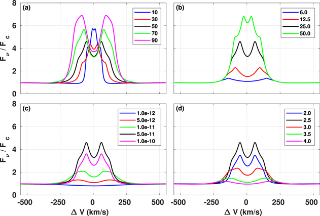
Figure 2. Example of the variation of the Hα emission line profiles by varying disk parameters. The reference model is shown in black in each panel for ease of comparison and corresponds to the disk parameters of n = 2.5,  g cm−3,
  R⋆, and
  . The fluxes are normalized to the continuum star+disk flux outside of the line. (a) Inclination variation. (b) Disk truncation radius variation. (c) Base density variation. (d) Power-law exponent variation.
Download figure:
Standard image High-resolution imageAs noted in the previous paragraph, the Hα line profiles shown as relative fluxes, i.e., divided by the predicted star+ disk continuum, can show a more complex behavior than might be expected because the line and continuum fluxes often have a different dependence on, say, the disk density. To clarify this point, Figure 3 shows the same line profiles as Figure 2 but plotted as absolute fluxes in janskys without continuum normalization. In panel (a) of Figure 3, the  profile is now the weakest and the
  profile is the strongest. The disk contribution to the normalizing continuum decreases in proportion to the disk’s projected area, i.e.,
  , while for large inclinations,
  , the stellar continuum can be significantly obscured by the circumstellar disk. In panel (b), there is a strong dependence of the line flux on RT, whereas the continuum flux is essentially independent of RT. This is because the continuum forms very close to the central star (inside of the
  , the smallest disk considered), whereas the optically thick Hα line emission forms over a much larger portion of the disk. In panel (c), the fluxes are now seen to scale in order with increasing
  , and the saturation of the line flux as compared to the continued increase in the continuum flux is clear. Finally, in panel (d), the line fluxes are ordered with increasing flux with decreasing n, and the dependence of the continuum flux with the density drop-off in the disk is as expected.
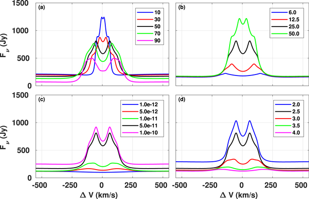
Figure 3. Same as Figure 2, but with the Hα lines plotted as absolute fluxes in janskys.
Download figure:
Standard image High-resolution imageFigure 2 suggests that there is some degeneracy among the calculated Hα line profiles, i.e., very similar relative flux line profiles can result from different combinations of the model parameters  . To explore this further, we have used the reference profile of Figure 2 corresponding to
  as a simulated observed profile and searched the B2V profile library for the top nine closest model profiles as defined by the smallest average percentage difference between the model and “observed” profile across the line: this figure of merit for the closeness of two line profiles is further discussed in the next section. Figure 4 shows the results. While all nine profiles share the same RT, there are small differences among the returned parameters, with n ranging between 2.0 and 2.5,
  between
  and
and  , and i between 40° and 60°. The variations in the parameters are correlated: typically, smaller
  values are associated with larger n values. In the next section, we describe how we deal with this degeneracy in assigning model parameters to each star.
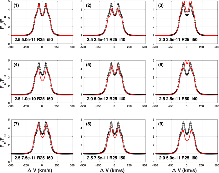
Figure 4. Top nine most similar profiles in the B2V Hα line library to the reference profile of Figure 2. The first panel is an identical match, whereas panels (2) through (9) represent increasing differences as measured by the average percentage difference between the two profiles. The model parameters  are as indicated at the bottom of each panel, and the reference parameters are those given in panel (1).
Download figure:
Standard image High-resolution image4. Results
4.1. Selection of the Best Disk Models
The Hα spectrum of each star in our sample was compared to the theoretical library for that spectral type using a script that systematically finds the best match to the observed profile. For each comparison, the percentage flux difference between the model and observation was averaged over the line to assign each comparison a figure-of-merit value (hereafter called  ), defined as

where Fiobs is the observed relative line flux,  is the model relative line flux, wi is a weight, discussed below, and the sum is over all wavelengths spanning the line. Several different weights were examined: uniform weighting wi = 1, line-center weighting
  , and uniform weighting but using the sum of the square of flux differences divided by flux. For each spectrum, we tested the second option first, but we also calculated the quality of the fits for other options as well, and by visual inspection we selected the best
  method to adopt for each spectrum (which may be different for each star) to use in our results.
Initially the best 50 matches out of the 1620 profiles using the smallest  values were identified, where
  is the minimum figure of merit of the best-fitting library profile. We show an example for a B2 spectral type in Figure 5 for the Be star HD 58343. The top left panel shows the best 50 models sorted by
  (black circles), with the best five models in red, blue, green, yellow, and cyan colors corresponding to
  of 1.00, 1.20, 1.30, 1.40, and 1.45, respectively. The best five models are different in the disk density parameters, but they have the same inclination angle, i = 10°, and the same disk truncation radius of
  for this star. The top right panel shows models of Hα line profiles corresponding to each respective color, as well as the observed profile shown in black. The main difference between these models appears in the flanks of the emission line. Hanuschik (1986) classified typical emission profiles seen in Be stars at different inclination angles, where this particular “wine bottle shape” is usually seen at low inclinations. Moreover, Hummel (1994) reproduced emission-line profiles using a Keplerian disk model for an optically thick disk (
 g cm−3), and he found for inclinations between 5° ≲ i ≲ 30° that emission-line profiles show inflection flanks. For high-inclination angles, i ≳ 75°, he noticed that a central depression plus a double-peak profile is generated, due to the velocity field present in the disk. The bottom left panel shows the behavior of
  versus
  , where, in this particular case, we can see that higher values of
  dominate. The bottom right panel is the same as the bottom left panel except for n. In Figure 5, the best model (red color) is well constrained by
  ; however, we notice that similar values of
  combined with different values of n give us similar profiles of the emission line (for the same inclination angle and same disk truncation radius). For this reason we consider a range of models within a percentage of
  as described in Section 4.3.

Figure 5. Example of the selection method. The results correspond to the Be star HD 58343 with an inclination angle of  and
and  R⋆. The first five best models are indicated with the
  value starting at 1.00 (red), 1.20 (blue), 1.30 (green), 1.40 (yellow), and 1.45 (cyan) in all panels. Top left:
  of the 50 best models. Top right: Hα line profiles models compared with the observation (black solid line). Bottom left:
  values for the best 50 models. Bottom right: n values for the best 50 models.
Download figure:
Standard image High-resolution image4.2. Best-fit Models by Visual Inspection
We chose the best model by visual inspection of the comparison plots between the models and the observations; such plots are shown in the
Table 2.
Summary of the Best-fit Model by Visual Inspection and Representative Models ( ) of Each Spectrum for Each Star
| Best Model | Observation | Representative Model | ||||||||||
|---|---|---|---|---|---|---|---|---|---|---|---|---|
| HD | SpT | Date |

|
i | n |

|
RT | EW |

|

|

|

|
| (yyyy mm dd) | (deg) | (g cm−3) | (R⋆) | ( ) ) |
(km s−1) | (R⋆) | ||||||
| (1) | (2) | (3) | (4) | (5) | (6) | (7) | (8) | (9) | (10) | (11) | (12) | (13) |
| 10144 | B6Vpe | 2012 Nov 13 | — | — | — | — | — | −0.8 | 719.5 | — | — | — |
| 2013 Jan 18 | 1.2 | 70 | 3.0 | 7.5e–12 | 6.0 | −0.9 | 485.1 | 10.4 | 1.8e–11 | 8.5e–10 | ||
| 2013 Jul 24 | 1.0 | 70 | 3.5 | 2.5e–11 | 6.0 | −0.5 | 361.8 | 13.5 | 2.8e–10 | 2.2e–08 | ||
| 2013 Oct 29 | 1.0 | 70 | 4.0 | 7.5e–11 | 6.0 | −1.2 | 353.6 | 14.6 | 4.0e–10 | 3.0e–08 | ||
| 2014 Jan 29 | 1.0 | 70 | 2.0 | 5.0e–11 | 6.0 | −1.7 | 345.3 | 12.9 | 3.3e–10 | 2.3e–08 | ||
| 33328(a) | B2IVne | 2012 Nov 13 | 1.0 | 60 | 4.0 | 7.5e–12 | 25.0 | 1.7 | 703.0 | — | — | — |
| 2013 Jan 18 | 1.0 | 60 | 4.0 | 2.5e–12 | 6.0 | 0.1 | 534.5 | — | — | — | ||
| 2015 Feb 25 | 1.0 | 60 | 4.0 | 7.5e–12 | 25.0 | 1.9 | 657.8 | — | — | — | ||
| 35165 | B2Vnpe | 2014/2015 blue | 1.0 | 80 | 2.0 | 5.0e–11 | 12.5 | −12.1 | 283.7 | 45.0 | 8.4e–10 | 1.0e–07 |
| 2014/2015 red | 1.1 | 80 | 2.0 | 1.0e–11 | 6.0 | −12.8 | 312.4 | 45.0 | 8.4e–10 | 1.0e–07 | ||
| 35411(a) | B1V + B2 | 2012 Nov 13 | 1.0 | 80 | 4.0 | 7.5e–12 | 25.0 | 2.15 | 0 | — | — | — |
| 2013 Jan 18 | 1.0 | 80 | 3.5 | 1.0e–12 | 50.0 | 3.1 | 0 | — | — | — | ||
| 2013 Feb 26 | 1.0 | 80 | 4.0 | 1.0e–12 | 6.0 | 3.0 | 0 | — | — | — | ||
| 2015 Feb 25 | 1.0 | 80 | 4.0 | 7.5e–12 | 25.0 | 2.4 | 0 | — | — | — | ||
| 35439(pf) | B1Vpe | 2012 Nov 13 | 1.0 | 50 | 2.5 | 2.5e–11 | 50.0 | −27.7 | 209.7 | — | — | — |
| 2013 Jan 18 | 1.0 | 50 | 2.5 | 2.5e–11 | 50.0 | −28.6 | 185.0 | — | — | — | ||
| 2013 Feb 26 | 1.0 | 50 | 2.5 | 2.5e–11 | 50.0 | −30.2 | 193.2 | — | — | — | ||
| 2015 Feb 25 | 1.0 | 70 | 2.0 | 5.0e–12 | 50.0 | −25.6 | 152.1 | — | — | — | ||
| 37795 | B9V | 2012 Nov 13 | 1.0 | 40 | 3.0 | 2.5e–10 | 50.0 | −9.3 | 106.9 | 46.4 | 3.8e–10 | 4.5e–08 |
| 2013 Jan 18 | 1.0 | 40 | 3.0 | 2.5e–10 | 50.0 | −9.7 | 82.2 | 53.3 | 4.5e–10 | 5.9e–08 | ||
| 2015 Feb 25 | 1.0 | 40 | 3.0 | 2.5e–10 | 50.0 | −9.0 | 82.2 | 50.2 | 4.0e–10 | 5.4e–08 | ||
| 41335(pf) | B2Vne | 2012 Nov 13 | 1.0 | 80 | 2.0 | 5.0e–12 | 25.0 | −25.9 | 152.1 | — | — | — |
| 2013 Jan 18 | 1.0 | 80 | 2.0 | 5.0e–12 | 25.0 | −27.1 | 111.0 | — | — | — | ||
| 2013 Feb 26 | 1.0 | 80 | 2.0 | 5.0e–12 | 25.0 | −26.7 | 115.1 | — | — | — | ||
| 2015 Feb 27 | 1.0 | 80 | 2.0 | 5.0e–12 | 25.0 | −26.9 | 115.1 | — | — | — | ||
| 42167 | B9IV | 2014 Jan 30 | 1.0 | 70 | 2.0 | 2.5e–10 | 6.0 | −2.0 | 160.3 | 32.6 | 5.8e–10 | 5.3e–08 |
| 2015 Feb 25 | 1.0 | 70 | 2.0 | 2.5e–10 | 6.0 | −1.7 | 209.7 | 32.6 | 5.8e–10 | 5.3e–08 | ||
| 45725 | B4Ve shell | 2015 Feb 26 | 1.0 | 70 | 2.0 | 5.0e–12 | 25.0 | −30.2 | 164.4 | 87.4 | 2.1e–09 | 3.7e–07 |
| 48917 | B2IIIe | 2014 Jan 29 | 1.0 | 60 | 2.0 | 5.0e–12 | 25.0 | −24.6 | 86.3 | 103.7 | 3.3e–09 | 6.3e–07 |
| 2015 Oct 23 | 1.0 | 60 | 2.0 | 5.0e–12 | 25.0 | −27.1 | 90.4 | 103.7 | 3.3e–09 | 6.3e–07 | ||
| 50013(pf) | B1.5Ve | 2012 Nov 13 | 1.0 | 50 | 2.5 | 2.5e–11 | 50.0 | −24.1 | 94.6 | — | — | — |
| 2013 Feb 26 | 1.0 | 60 | 2.0 | 5.0e–12 | 50.0 | −22.2 | 98.7 | — | — | — | ||
| 2014 Mar 21 | 1.0 | 50 | 2.5 | 2.5e–11 | 50.0 | −24.0 | 65.8 | — | — | — | ||
| 2015 Feb 25 | 1.0 | 60 | 2.0 | 5.0e–12 | 50.0 | −25.2 | 65.8 | — | — | — | ||
| 2015 Oct 23 | 1.0 | 60 | 2.0 | 5.0e–12 | 50.0 | −28.9 | 74.0 | — | — | — | ||
| 52918(a) | B1V | 2014 Jan 29 | 1.0 | 60 | 4.0 | 1.0e–11 | 25.0 | 1.37 | 678.4 | — | — | — |
| 56014 | B3IIIe | 2014 Jan 29 red | 1.0 | 80 | 2.5 | 1.0e–11 | 6.0 | −2.0 | 390.6 | 23.4 | 3.0e–10 | 2.7e–08 |
| 2014 Jan 29 blue | 1.0 | 80 | 2.5 | 5.0e–12 | 12.5 | −2.0 | 390.6 | 23.4 | 3.0e–10 | 2.7e–08 | ||
| 56139 | B2IV–Ve | 2013 Feb 27 | 1.0 | 30 | 2.0 | 2.5e–11 | 25.0 | −20.7 | 0 | 105.5 | 9.1e–09 | 1.7e–06 |
| 2015 Feb 27 | 1.0 | 30 | 2.0 | 2.5e–11 | 25.0 | −16.7 | 0 | 105.5 | 9.1e–09 | 1.7e–06 | ||
| 2015 Nov 14 | 1.0 | 30 | 2.0 | 5.0e–11 | 25.0 | −10.2 | 0 | 73.7 | 1.4e–08 | 2.3e–06 | ||
| 57150 | B2Ve + B3IVne | 2014 Jan 29 | 1.0 | 60 | 2.0 | 5.0e–12 | 50.0 | −30.2 | 0 | 189.2 | 6.8e–09 | 1.8e–06 |
| 57219(a) | B3Vne | 2014 Jan 29 | 1.0 | 80 | 3.5 | 7.5e–12 | 25.0 | 2.3 | 0 | — | — | — |
| 58343 | B2Vne | 2013 Feb 27 | 1.0 | 10 | 2.5 | 7.5e–11 | 25.0 | −7.2 | 0 | 71.7 | 7.7e–09 | 1.2e–06 |
| 58715 | B8Ve | 2013 Feb 27 | 1.0 | 50 | 3.5 | 2.5e–10 | 25.0 | −7.2 | 127.4 | 35.6 | 1.2e–09 | 1.2e–07 |
| 2015 Feb 25 | 1.0 | 50 | 3.5 | 2.5e–10 | 25.0 | −7.3 | 115.1 | 35.6 | 1.2e–09 | 1.2e–07 | ||
| 60606 | B2Vne | 2012 Nov 13 | 1.0 | 70 | 3.0 | 1.0e–10 | 25.0 | −21.3 | 143.9 | 62.2 | 3.2e–09 | 5.1e–07 |
| 2013 Jan 19 | 1.0 | 70 | 3.0 | 1.0e–10 | 25.0 | −22.8 | 152.1 | 62.2 | 3.2e–09 | 5.1e–07 | ||
| 2013 Feb 26 | 1.0 | 70 | 3.0 | 1.0e–10 | 25.0 | −18.9 | 135.7 | 62.2 | 3.2e–09 | 5.1e–07 | ||
| 63462(pf) | B1IVe | 2013 Feb 27 | 1.0 | 70 | 2.0 | 5.0e–12 | 12.5 | −10.9 | 94.6 | — | — | — |
| 2015 Oct 23 | 1.0 | 50 | 2.5 | 1.0e–11 | 50.0 | −11.6 | 94.6 | — | — | — | ||
| 68423 | B6Ve | 2014 Mar 21 | 1.0 | 10 | 2.0 | 2.5e–10 | 50.0 | −6.2 | 49.3 | 49.1 | 1.1e–08 | 1.4e–06 |
| 68980 | B1.5III | 2013 Feb 27 | 1.0 | 40 | 2.0 | 5.0e–12 | 50.0 | −23.2 | 41.1 | 214.2 | 1.1e–08 | 2.9e–06 |
| 2015 Feb 26 | 1.0 | 40 | 2.5 | 2.5e–11 | 50.0 | −19.6 | 45.2 | 130.2 | 1.3e–08 | 3.0e–06 | ||
| 71510(a) | B2Ve | 2014 Jan 29 | 1.0 | 70 | 3.0 | 2.5e–12 | 12.5 | 2.6 | 0 | — | — | — |
| 2014 Mar 19 | 1.0 | 70 | 4.0 | 7.5e–12 | 6.0 | 2.6 | 0 | — | — | — | ||
| 2015 Feb 26 | 1.0 | 70 | 2.0 | 1.0e–12 | 6.0 | 2.25 | 0 | — | — | — | ||
| 75311 | B3Vne | 2014 Mar 19 | 1.0 | 60 | 3.0 | 7.5e–11 | 50.0 | −0.6 | 287.8 | 26.0 | 2.8e–09 | 2.7e–07 |
| 78764 | B2IVe | 2014 Jan 30 | 1.0 | 40 | 2.5 | 7.5e–11 | 12.5 | −4.8 | 131.6 | 42.1 | 3.6e–09 | 5.3e–07 |
| 2014 Mar 19 | 1.0 | 40 | 2.5 | 7.5e–11 | 12.5 | −4.2 | 139.8 | 42.1 | 3.6e–09 | 5.3e–07 | ||
| 83953(pf) | B5V | 2013 Feb 27 | 1.0 | 70 | 3.0 | 1.0e–10 | 50.0 | −20.6 | 160.3 | — | — | — |
| 89080 | B8IIIe | 2013 Feb 27 | 1.1 | 70 | 2.0 | 2.5e–12 | 25.0 | −7.2 | 164.4 | 35.6 | 8.8e–10 | 8.8e–08 |
| 2014 May 09 | 1.1 | 70 | 2.0 | 2.5e–12 | 25.0 | −7.0 | 143.9 | 35.6 | 8.8e–10 | 8.8e–08 | ||
| 89890(a) | B3IIIe | 2014 Jan 30 | 1.0 | 70 | 3.0 | 5.0e–12 | 50.0 | 1.7 | 0 | — | — | — |
| 2014 Mar 19 | 1.0 | 80 | 3.5 | 7.5e–12 | 25.0 | 2.3 | 0 | — | — | — | ||
| 2015 Feb 27 | 1.0 | 80 | 3.0 | 5.0e–12 | 50.0 | 1.7 | 0 | — | — | — | ||
| 2015 May 06 | 1.0 | 70 | 3.5 | 7.5e–12 | 25.0 | 1.9 | 0 | — | — | — | ||
| 91465 | B4Vne | 2013 Feb 26 | 1.0 | 70 | 2.0 | 5.0e–12 | 25.0 | −28.4 | 131.6 | 82.4 | 2.4e–09 | 3.8e–07 |
| 2014 May 09 | 1.0 | 70 | 2.0 | 1.0e–10 | 50.0 | −24.9 | 135.7 | 63.1 | 2.1e–09 | 3.1e–07 | ||
| 2015 Feb 27 | 1.0 | 70 | 2.0 | 1.0e–10 | 50.0 | −22.9 | 94.6 | 63.1 | 2.1e–09 | 3.1e–07 | ||
| 2015 May 06 | 1.1 | 70 | 2.0 | 5.0e–12 | 25.0 | −30.4 | 98.7 | 97.4 | 2.9e–09 | 5.0e–07 | ||
| 92938(a) | B4V | 2014 Jan 30 | 1.0 | 80 | 4.0 | 7.5e–12 | 12.5 | 2.4 | 0 | — | — | — |
| 2015 Feb 27 | 1.0 | 80 | 4.0 | 7.5e–12 | 12.5 | 2.6 | 0 | — | — | — | ||
| 2015 May 06 | 1.0 | 80 | 4.0 | 7.5e–12 | 12.5 | 4.3 | 0 | — | — | — | ||
| 93563 | B8.5IIIe | 2014 Jan 30 | 1.2 | 70 | 3.5 | 1.0e–10 | 50.0 | −8.1 | 296.0 | 22.5 | 6.3e–11 | 5.0e–09 |
| B8.5IIIe | 2015 May 06 | 1.2 | 70 | 3.5 | 1.0e–10 | 50.0 | −9.7 | 135.7 | 22.5 | 6.3e–11 | 5.0e–09 | |
| 102776 | B3Vne | 2014 Jan 30 | 1.0 | 60 | 3.0 | 5.0e–11 | 50.0 | −12.2 | 98.7 | 52.1 | 9.6e–10 | 1.2e–07 |
| 2014 Mar 19 | 1.0 | 60 | 2.5 | 1.0e–11 | 50.0 | −9.7 | 185.0 | 90.6 | 9.4e–10 | 1.7e–07 | ||
| 2015 Feb 27 | 1.1 | 60 | 2.0 | 2.5e–12 | 25.0 | −7.1 | 185.0 | 85.5 | 1.3e–09 | 2.3e–07 | ||
| 2015 May 06 | 1.0 | 60 | 2.0 | 2.5e–12 | 50.0 | −7.4 | 119.2 | 91.4 | 2.0e–09 | 3.5e–07 | ||
| 103192 | B9IIIsp | 2014 Mar 19 | 1.2 | 60 | 3.0 | 7.5e–12 | 50.0 | −1.4 | 259.0 | 13.4 | 4.6e–10 | 3.4e–08 |
| 2015 Feb 26 | 1.2 | 60 | 3.0 | 7.5e–12 | 50.0 | 1.2 | 263.1 | 13.4 | 4.6e–10 | 3.4e–08 | ||
| 2015 May 07 | 1.2 | 60 | 3.0 | 7.5e–12 | 50.0 | 2.0 | 234.3 | 13.4 | 4.6e–10 | 3.4e–08 | ||
| 105382(a) | B6IIIe | 2014 Jan 30 | 1.0 | 80 | 3.5 | 5.0e–12 | 25.0 | 1.3 | 0 | — | — | — |
| 2015 May 07 | 1.0 | 80 | 3.0 | 2.5e–12 | 25.0 | 2.5 | 0 | — | — | — | ||
| 105435 | B2Vne | 2014 Jan 30 | 1.0 | 60 | 2.5 | 1.0e–10 | 50.0 | −37.0 | 0 | 157.9 | 1.0e–08 | 2.3e–06 |
| 2015 Feb 25 | 1.0 | 60 | 2.0 | 5.0e–12 | 50.0 | −33.1 | 0 | 198.5 | 9.1e–09 | 2.4e–06 | ||
| 2015 May 06 | 1.0 | 60 | 2.0 | 5.0e–12 | 50.0 | −31.0 | 0 | 198.5 | 9.1e–09 | 2.4e–06 | ||
| 107348 | B8Ve | 2014 Jan 30 | 1.0 | 50 | 3.0 | 2.5e–10 | 25.0 | −10.2 | 82.2 | 30.1 | 1.5e–09 | 1.5e–07 |
| 2015 May 07 | 1.1 | 50 | 3.0 | 5.0e–11 | 25.0 | −6.9 | 123.3 | 37.4 | 1.0e–09 | 1.0e–07 | ||
| 110335 | B6IVe | 2014 Jan 30 | 1.1 | 70 | 3.0 | 2.5e–10 | 25.0 | −19.3 | 69.9 | 55.8 | 2.1e–09 | 2.8e–07 |
| 2015 May 07 | 1.1 | 70 | 3.0 | 2.5e–10 | 25.0 | −18.3 | 90.4 | 55.8 | 2.1e–09 | 2.8e–07 | ||
| 110432(pf) | B0.5IVpe | 2014 Jan 31 | 1.0 | 80 | 2.0 | 7.5e–12 | 25.0 | −30.2 | 197.3 | — | — | — |
| 2015 May 06 | 1.0 | 80 | 2.0 | 7.5e–12 | 25.0 | −28.6 | 102.8 | — | — | — | ||
| 112078(a) | B3Vne | 2014 Jan 31 | 1.0 | 30 | 2.5 | 1.0e–12 | 50.0 | 2.2 | 0 | — | — | — |
| 120324 | B2Vnpe | 2014 Jan 31 | 1.0 | 50 | 2.0 | 5.0e–11 | 25.0 | −14.8 | 74.0 | 72.8 | 7.6e–09 | 1.2e–06 |
| 2015 Feb 25 | 1.0 | 50 | 2.5 | 7.5e–11 | 25.0 | −18.6 | 66.8 | 78.4 | 3.9e–09 | 5.7e–07 | ||
| 2015 May 06 | 1.1 | 50 | 2.5 | 5.0e–11 | 25.0 | −21.0 | 0 | 97.0 | 4.0e–09 | 7.2e–07 | ||
| 124195(a) | B5V | 2014 Mar 21 | 1.0 | 70 | 4.0 | 7.5e–12 | 50.0 | 2.2 | 0 | — | — | — |
| 124367 | B4Vne | 2014 Jan 31 | 1.1 | 70 | 2.0 | 5.0e–12 | 50.0 | −38.9 | 98.7 | 21.7 | 1.4e–09 | 1.2e–07 |
| 124771(a) | B4V | 2014 Mar 21 | 1.1 | 70 | 4.0 | 5.0e–12 | 6.0 | 2.1 | 0 | — | — | — |
| 127972 | B2Ve | 2014 Jan 31 | 1.0 | 80 | 2.5 | 7.5e–12 | 12.5 | −5.3 | 259.0 | 26.9 | 3.0e–10 | 2.8e–08 |
| 2015 Feb 25 | 1.0 | 80 | 2.5 | 7.5e–12 | 12.5 | −3.7 | 349.5 | 26.9 | 3.0e–10 | 2.8e–08 | ||
| 2015 Jul 15 | 1.0 | 80 | 2.5 | 7.5e–12 | 12.5 | −2.9 | 365.9 | 26.9 | 3.0e–10 | 2.8e–08 | ||
| 131492 | B4Vnpe | 2014 Mar 21 | 1.0 | 70 | 3.0 | 1.0e–11 | 6.0 | −0.9 | 489.2 | 21.7 | 1.4e–09 | 1.2e–07 |
| 135734 | B8Ve | 2013 Jul 24 | 1.1 | 60 | 2.0 | 2.5e–12 | 25.0 | −7.0 | 168.6 | 40.2 | 1.1e–09 | 1.2e–07 |
| 2015 Feb 25 | 1.1 | 60 | 2.5 | 1.0e–11 | 25.0 | −8.3 | 135.7 | 40.2 | 1.1e–09 | 1.2e–07 | ||
| 2015 Jul 15 | 1.1 | 60 | 2.5 | 1.0e–11 | 25.0 | −8.2 | 152.1 | 40.2 | 1.1e–09 | 1.2e–07 | ||
| 138769(a) | B3IVp | 2013 Jul 24 | 1.0 | 80 | 2.5 | 1.0e–12 | 12.5 | 4.2 | 0 | — | — | — |
| 2015 Jul 15 | 1.0 | 80 | 3.5 | 5.0e–12 | 50.0 | 3.1 | 0 | — | — | — | ||
| 142184(a) | B2V | 2013 Jul 24 | 1.0 | 60 | 4.0 | 5.0e–12 | 12.5 | 2.0 | 698.9 | — | — | — |
| 2014 Mar 21 | 1.0 | 80 | 4.0 | 2.5e–12 | 6.0 | 3.5 | 698.9 | — | — | — | ||
| 143275 | B0.3IV | 2014 Mar 19 | 1.1 | 20 | 3.0 | 7.5e–11 | 50.0 | −11.3 | 0 | 143.6 | 1.0e–07 | 3.1e–05 |
| 148184 | B2Ve | 2013 Jul 24 | 1.0 | 30 | 2.0 | 1.0e–11 | 25.0 | −35.9 | 0 | 152.8 | 2.4e–08 | 5.5e–06 |
| 2015 Feb 25 | 1.0 | 30 | 2.0 | 1.0e–11 | 25.0 | −34.9 | 0 | 152.8 | 2.4e–08 | 5.5e–06 | ||
| 2015 May 06 | 1.0 | 30 | 2.0 | 1.0e–11 | 25.0 | −39.9 | 0 | 152.8 | 2.4e–08 | 5.5e–06 | ||
| 157042 | B2IIIne | 2013 Jul 24 | 1.1 | 70 | 2.5 | 2.5e–11 | 12.5 | −20.2 | 160.3 | 55.0 | 1.6e–09 | 2.1e–07 |
| 2015 May 06 | 1.1 | 70 | 2.5 | 2.5e–11 | 12.5 | −22.9 | 213.8 | 55.0 | 1.6e–09 | 2.1e–07 | ||
| 158427 | B2Ve | 2015 May 06 | 1.0 | 70 | 2.0 | 5.0e–12 | 50.0 | −36.1 | 32.9 | 188.1 | 7.5e–09 | 2.0e–06 |
| 167128 | B3IIIpe | 2013 Jul 24 | 1.0 | 40 | 3.5 | 7.5e–11 | 50.0 | −3.8 | 164.4 | 32.6 | 3.1e–09 | 3.9e–07 |
| 205637 | B3V | 2012 Nov 14 | 1.1 | 89 | 2.0 | 1.0e–11 | 6.0 | −1.9 | 337.1 | 27.3 | 8.8e–10 | 8.4e–08 |
| 209014 | B8Ve | 2013 Jul 24 | 1.0 | 89 | 2.0 | 2.5e–10 | 12.5 | −8.0 | 242.6 | 29.3 | 1.1e–09 | 1.1e–07 |
| 2015 Oct 23 | 1.0 | 89 | 2.0 | 2.5e–10 | 12.5 | −8.5 | 209.7 | 29.3 | 1.1e–09 | 1.1e–07 | ||
| 209409 | B7IVe | 2012 Nov 13 | 1.0 | 80 | 2.0 | 5.0e–12 | 25.0 | −18.9 | 143.9 | 58.2 | 7.9e–10 | 1.1e–07 |
| 2015 Oct 24 | 1.2 | 80 | 2.0 | 5.0e–12 | 50.0 | −20.0 | 152.1 | 55.6 | 2.0e–09 | 2.4e–07 | ||
| 212076 | B2IV–Ve | 2012 Nov 13 | 1.3 | 30 | 2.0 | 2.5e–11 | 25.0 | −18.2 | 28.8 | 85.1 | 3.1e–09 | 4.8e–07 |
| 2015 Oct 23 | 1.0 | 30 | 2.0 | 2.5e–12 | 50.0 | −14.3 | 24.7 | 118.2 | 6.8e–09 | 1.2e–06 | ||
| 212571 | B1III–IV | 2012 Nov 14 | 1.1 | 60 | 2.5 | 1.0e–11 | 12.5 | −7.7 | 283.7 | 84.1 | 9.3e–10 | 1.5e–07 |
| 2013 Jul 24 | 1.1 | 60 | 2.5 | 7.5e–12 | 12.5 | −4.0 | 304.2 | 74.4 | 6.4e–10 | 9.6e–08 | ||
| 2015 Oct 24 | 1.0 | 60 | 2.5 | 1.0e–11 | 12.5 | −10.7 | 209.7 | 83.9 | 1.6e–09 | 2.6e–07 | ||
| 214748 | B8Ve | 2012 Nov 15 | 1.3 | 50 | 3.5 | 2.5e–10 | 12.5 | −4.0 | 131.6 | 28.7 | 2.8e–09 | 2.2e–07 |
| 2013 Jul 24 | 1.3 | 50 | 3.5 | 2.5e–10 | 12.5 | −4.9 | 123.3 | 28.7 | 2.8e–09 | 2.2e–07 | ||
| 2015 Jul 15 | 1.3 | 50 | 3.5 | 2.5e–10 | 12.5 | −5.7 | 123.3 | 28.7 | 2.8e–09 | 2.2e–07 | ||
| 2015 Oct 24 | 1.3 | 50 | 3.5 | 2.5e–10 | 12.5 | −5.7 | 135.7 | 28.7 | 2.8e–09 | 2.2e–07 | ||
| 217891 | B6Ve | 2012 Nov 13 | 1.0 | 40 | 2.0 | 5.0e–11 | 50.0 | −21.1 | 0 | 94.1 | 1.7e–08 | 2.9e–06 |
| 2013 Jul 25 | 1.0 | 40 | 2.0 | 5.0e–11 | 50.0 | −22.8 | 0 | 94.1 | 1.7e–08 | 2.9e–06 | ||
| 219688(a) | B5V | 2015 Oct 24 | 1.0 | 50 | 3.0 | 2.5e–12 | 12.5 | 2.6 | 0 | — | — | — |
| 221507(a) | B9.5IIIp HgMnSi | 2013 Jul 24 | 1.0 | 89 | 3.0 | 2.5e–12 | 6.0 | 2.5 | 0 | — | — | — |
| 2015 Jul 15 | 1.0 | 89 | 3.0 | 2.5e–12 | 6.0 | 3.5 | 0 | — | — | — | ||
| 2015 Oct 23 | 1.0 | 89 | 3.0 | 2.5e–12 | 6.0 | 4.1 | 0 | — | — | — | ||
| 224686 | B8Ve | 2012 Nov 13 | 1.0 | 80 | 2.0 | 2.5e–10 | 6.0 | −2.0 | 275.4 | 28.7 | 2.8e–9 | 2.8e–07 |
Notes. The reader is referred to Section 4.2 for the selection details. The information displayed in this table is for the best (visual inspection) and representative ( ) models of each observation. Values of the representative models are only for emission profiles without a poor fit. The spectral type (SpT) is obtained from the SIMBAD database. Blue and red (indicated next to the date) refer to the blue and red peak fit, respectively. a: absorption profiles; pf: poor fit; dash: not agreement model.
Targets are sorted by HD number, indicating the date of the observation and the  value of the chosen model. Table 2 also lists the Hα equivalent width, EW, and the emission double-peak separation,
  , measured from the observations. Some of the targets are represented by more than one observation, due to variability, and they show changes in the line profile (peak height, violet-to-red peak ratio, etc). There are 22 such variable cases indicated by an asterisk beside the star name below the plot (14 of these are in emission and 8 in absorption), and they were treated by keeping the inclination angle constant for the system, and each time fit with different models. In our program stars there are 15 Be stars with Hα in absorption. We notice that in our sample all targets are confirmed as Be stars, so absorption profiles presented here are Be stars in diskless phase or currently without a disk. We did not include absorption profiles in our analysis; nevertheless, our spectral library contains profiles with pure photospheric Hα profiles.
We provide our results separately for the emission profiles, for the absorption lines, and for the targets with poor fits. Overall, we have 42 Be stars with Hα emission, 15 with absorption profiles, and 6 with poor fits. All systems are displayed in the
4.3. Distribution of the Disk Density Parameters: Representative Models
In the previous section, we determined the best-fit disk density models for each of our program stars with Hα in emission. In this section, we wish to look at the distribution of disk density parameters in this sample. From now on, every spectrum in emission for each target (if there is more than one) is considered by a separate, unique model. This give us a total of 61 emission models. As we explained in the previous section, there are a range of models for each star that fit the observed profile nearly as well as the best-fit model selected by visual inspection. Thus, for any given star, we can systematically define a “set” of best-fit parameters by selecting all models with  , resulting in N models being selected. We note that by selecting a slightly larger range of
  , as Figure 5 demonstrates, the base density and the exponent of the disk surface density span a wide range of values especially for
  . To define representative disk density parameters for each star, we choose a weighted average over the N selected models. For the disk parameter X, which could be
  or n, etc., we define

where  and the weights are chosen as

The index m was chosen to be equal to −10 so that significantly different weights are given to models ranging from 1 to 1.25, i.e., the weight assigned to  is
is  . This procedure was applied to all the physical quantities obtained from the emission profiles, which are presented below. In order to study the conditions under which the disk exists and its link with the spectral type, we distinguish in our study between early-type (B0–B3) and late-type (B4–B9) Be stars.
The representative values (weighted average) of the parameters governing the disk density (n and  in Equation (1)) of emission profiles are displayed in Figure 5. The most frequent pairs are concentrated in the range
  and
and  or
or  to −10.2.
We note that we detect emission profiles in the upper left triangular region of Figure 6. With increasing values of the density exponent and decreasing base density, corresponding to the lower right in Figure 6, it would be increasingly difficult to detect emission, due to reduced disk density. The lack of disk material for these stars made it impossible to constrain our models, as mentioned above, so we did not analyze any features for them. Moreover, some absorption profiles seemed to be pure photospheric lines, and some showed evidence of a possible formation/dissipation disk phase (see HD 33328's spectrum, for example, in the

Figure 6. Distribution of the representative  and
and  model values for systems with emission profiles.
Download figure:
Standard image High-resolution image4.4. Distribution of Disk Mass and Angular Momentum
From each star’s fitted disk density parameters, we can estimate the mass of the disk by integrating the disk density law, Equation (1), over the volume of the disk. For the radial extent of the disk, we chose the radius that encloses 90% of the total flux of the Hα line in an  (i.e., face-on disk) image computed with BERAY. This measure of the Hα disk size was used in favor of the fitted RT, as the latter was computed on a very coarse grid of only four values. To compute each disk mass,
  , the representative values of the disk parameters were used, which included the models with
  . In addition to disk mass, the representative value of the total angular momentum content,
  , of each disk was also computed, using the same disk density parameters and assuming pure Keplerian rotation for the disk. Representative values of the disk mass and angular momentum in stellar units are displayed in Table 2 in columns (12) and (13), respectively.
Figure 7 shows the distribution of both representative values, disk mass and disk specific angular momentum,  , for early and late stellar types. To normalize by the stellar angular momentum, the central star was assumed to rotate as a solid body at
  , with the critical velocity computed using Equation (4). (See also Section 5.3 for a discussion about the effect of the stellar rotation on Jd.)
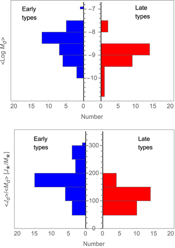
Figure 7. Distribution of the representative values of the disk mass (top panel) and angular momentum of the disk (bottom panel) compared to the central star.
Download figure:
Standard image High-resolution imageThe distribution of the disk mass in early types ranges from  to
to  (see top panel in Figure 7). For late types, values range from
  to
to  . The mean disk mass for the early types is
  , while for the late types, the mean disk mass is
  .
.
The bottom panel in Figure 7 shows the distribution of the specific angular momentum  of the disk in units of stellar specific angular momentum. For early types, the most frequent range is
  and corresponds to a
  and a total mass of
  . For late types the most frequent values range from 100 to 150, corresponding to a range of
  and
and  . In general, late types have lower values of
  and
and  in comparison with early types. It should be kept in mind that while the model disk masses vary over a large range (with
  spanning
  to
to  ), the range of model specific angular momentum is much less owing to the assumption of Keplerian rotation. The minimum and maximum values of
  in units of
  are 49 and 306, for a total variation of just over a factor of 6.
4.5. Relation between Hα Equivalent Width and Disk Mass
The relation between Hα EW and disk mass,  , separated by early- and late-type Be stars, is shown in Figure 8. Negative values indicate that the net flux of the emission line is above the continuum level. While there is an overall trend for the most massive disks to have the largest Hα EW, there is an extremely large dispersion. This is not unexpected; for any given power-law index n in Equation (1), the Hα EW will first increase with
  , reach a maximum, and then decline (see, e.g., Sigut et al. 2015). This decline occurs because once the density becomes large enough, the continuum flux from the disk at the wavelength of Hα rises more quickly than the line emission, so the equivalent width actually decreases with
  , as does the corresponding disk mass. The exact value of
  at which the Hα equivalent width peaks is dependent on n; therefore, in a mix of models with differing
  , there will not be a direct relationship between disk mass and Hα EW. Finally, we note that the most massive disks and largest Hα equivalent widths (absolute value) are found most frequently among the early-type Be stars.

Figure 8. Equivalent widths of the Hα emission line profiles as a function of mass.
Download figure:
Standard image High-resolution image5. Discussion
5.1. Disk Density
We found a distribution of the representative values of the disk density parameters for early and late spectral types, which are displayed in Figure 6. Early stellar types cover values of  between 2.0 and 3.0, while late stellar types reach values near 3.7. It appears that higher values of the power-law exponent are found for stars with lower effective temperature. This could explain the small emission disks seen in late-type stars since with increasing n the disk density falls faster with distance from the star. However, the average values of the representative values of the power-law exponent are essentially the same for early and late spectral types:
  and
and  .
.
Previous work in the literature using BEDISK was completed by Silaj et al. (2010). They created a grid of disk models for B0, B2, B5, and B8 stellar types at three inclinations angles  , 45°, and 70° for different disk densities. They modeled Hα line profiles of a set of 56 Be stars (excluding Be-shell stars) and studied the effects of the density and temperature in the disk. Their results show a higher percentage of models with
  ranging between 10−11 and
  and a significant peak of
  , which is slightly larger than the values of n found in this study. We attribute this difference to the different methods used to compute the Hα line profile. Silaj et al. (2010) used BEDISK to compute the line intensity escaping perpendicular to the equatorial plane in each disk annulus (i.e., rays for which
  ). They then assumed that this ray was representative of other angles considered, i = 20°, 45°, and 70°, and combined the
  rays with the appropriate Doppler shifts and projected areas. Clearly this computation method becomes limited with larger viewing angles. In contrast, BERAY, used here, does not make any of these approximations, and it has been successfully used to model the Hα lines of Be-shell stars for which the inclination angle is large (Silaj et al. 2014b). Eight Be-shell spectra were analyzed, and values for
  between 10−12 and 10−10 g cm−3 and n between 2.5 and 3.5 were found.
Touhami et al. (2011) used the assumption of an isothermal disk and the same density prescription as Equation (1) to reproduce the color excess in the near-infrared (NIR) of a sample of 130 Be stars. For the central star, they assumed an early-type star and adopted  for all the models. They varied
  between 10−12 and 2.0 × 10⁻¹⁰ g cm−3, which is very similar to our range of
  variation. They set the inclination angle at i = 45° and 80° and used an outer disk radius of ∼14.6R⋆ and 21.4R⋆. Other studies also use the same scenario for the density distribution, where the base density of the disk is found to be between 10−12 and 10−10 g cm−3 and the power-law exponent n is usually in the range of 2–4 (for a review of recent results the reader is referred to Section 5.1.3 of Rivinius et al. 2013b).
Recently, Vieira et al. (2017) determined the disk density parameters  and n for 80 Be stars observed in different epochs, corresponding to 169 specific disk structures. They used the viscous decretion disk model to fit the infrared continuum emission of their observations, using infrared wavelengths. They found that the exponent n is in the range between 1.5 and 3.5, where our most frequent values are between 2.0 and 2.5 for both early and late spectral types. They also found
  to range between 10−12 and 10−10 g cm−3, which compares favorably with our average values of (4.00–6.30) × 10−11 g cm−3, again for both early and late spectral types. Vieira et al. (2017) also established that the disks around early-type stars are denser than in late-type stars, consistent with our finding of more massive disks for the earlier spectral types.
Finally, we also notice that our models sometimes do not reproduce the wings of our Hα observations. This may reflect our assumption of a single radial power law for the equatorial density variation in this disk. Alternatively, for earlier spectral types, this may reflect neglect of noncoherent electron scattering in the formation of Hα (Poeckert & Marlborough 1979). For example, Delaa et al. (2011) performed an interferometric study of two Be stars using a kinematic disk model neglecting the expansion in the equatorial disk. They were able to fit the wings and the core of the Hα emission line by introducing a factor to estimate the incoherent scattering to their kinematic model.
5.2. Size of the Emission Region
The outer extent of the disk considered in the modeling of this work was assumed to be one of four values, 6.0R⋆, 12.5R⋆, 25.0R⋆, and 50.0R⋆. From these values, the best-fitting models have a disk truncation radius of 25.0R⋆ followed by 50.0R⋆. Nevertheless, as noted previously, a better estimate of the size of the Hα-emitting region is the equatorial radius that contains 90% of the integrated Hα flux in an  image computed with BERAY, a quantity we denotes as R90. We provide R90 values in column (11) of Table 2. These values, based on the integrated flux from our models, could be used by other studies to conveniently compare with our results.
As an additional check, we compare our R90 disk sizes with a measure based on the observed separation of the Hα emission peaks, as first suggested by Huang (1972), and tailored to our model assumptions. The basic idea of this method is that the double-peak separation is set by the disk velocity at its outer edge, which we will denote RH. If the observed peak separation is  , we have

assuming Keplerian rotation for the disk and correcting the observed peak separation for the viewing inclination i. Hence,
In this work, we assumed that all Be stars rotate at 80% of their critical velocity; therefore, each star’s equatorial velocity is

where  is the stellar (polar) radius. Using this to eliminate
  from the previous equation and solving for the disk size, we have

As  is the star’s
  value, we have approximately

This equation is very similar to the form used by many authors to derive approximate disk sizes from observed spectra (e.g., Hanuschik 1986; Hummel 1994). We note that the way we use Equation (12) is slightly nonstandard: we do not measure  directly from our spectra; instead, we adopt the
  of the best-fit model. As the Hα profiles are essentially insensitive to
  , we are using the observed peak separation
  and the best-fit value of i for the viewing inclination.
The correlation between RH and R90 is displayed in Figure 9. For a few of our targets, we do not obtain an RH value because of a small  or small inclination where Huang’s law is not valid. The solid line indicates the linear fit over both early (blue circles) and late (red squares) stellar types, considering values not larger than 50.0R⋆ and greater than 1R⋆ to be consistent with the input values used in the BERAY model. The relation between the representative values of the mentioned sizes is given by the linear equation
  in units of stellar radius, with a correlation of rcorr = 0.611 with confidence intervals calculated using a bootstrapping method. We notice that the most frequent disk size values calculated by Huang’s relation for early and late spectral types are concentrated less than 5R⋆ and the values containing 90% of the Hα flux for early and late spectral types are concentrated between 10R⋆ and 15R⋆.

Figure 9. Relation between the emitting size containing 90% of the integrated Hα emission, R90, and the emitting size obtained from Huang’s law, RH. A linear fit is represented by the solid line.
Download figure:
Standard image High-resolution imageMany other measurements of the Be star disk sizes have been reported in the literature. Hanuschik (1986) measured the  and the FWHM in the Hα emission line of 24 southern Be stars, and using Huang’s law, he estimated an outer emitting size of ∼10R⋆. Similar values were found by Slettebak et al. (1992) for 41 Be stars; they obtained an outer emitting size in the range ∼7R⋆–19R⋆ for the Hα emission line. Using interferometric techniques, Tycner et al. (2005) studied the relation between the total flux emission of Hα line and the physical size of the emission region in seven Be stars, finding for the first time a clear correlation between both these quantities. For early stellar types they found an extended emitting size of ∼18.0R⋆ to 21.0R⋆, while for stars with lower effective temperatures they found smaller values of ∼6.0R⋆ to 14.0R⋆ (with an exception for ψ Per of ∼32.0R⋆). An alternative way to estimate the emitting region based on the Hα half-width at half-maximum was proposed by Grundstrom & Gies (2006). They compared their results with the interferometric measures of the Hα-emitting size in the literature and obtained lower values between ∼5.0R⋆ and 10.0R⋆.
Our very low values of RH from observed emission profiles (less than 1R⋆ and not considered in the analysis) come from very large  values. If the star is rotating near its critical rotation, the gas could accumulate near the star, and consequently the emission region of the Hα line could be of the order of a few stellar radii.
Overall, our results for RT, either from the representative models or from Huang’s law, show general agreement with previous works in the literature, giving higher values for early stellar types and lower values for late Be types.
5.3. Mass and Angular Momentum of the Disk
In Section 4.4 we provided the range of the total disk mass and the total disk angular momentum for early and late stellar types. Our results gave us higher values of  and
and  for early types in comparison with late types. This was expected considering that late stellar types have, in general, smaller disks. Considering the whole sample without distinction between early and late stellar types, we estimate that the total angular momentum content in the disk is approximately 10−7 times the angular momentum of the central star and the mass of the disk is approximately 10−9 times the mass of the central star.
Sigut et al. (2015) studied the disk properties of the late Be-shell star Omicron Aquarii (o Aqr, B7IVe) combining contemporaneous interferometric and spectroscopy Hα observations with NIR spectral energy distributions. They compared the values obtained by each technique for different disk parameters. From Hα spectroscopy, values of RT, Md, and Jd are higher than those obtained from the NIR, while  and n are lower than NIR. From their results, the comparison between values obtained from spectroscopy, interferometry, and NIR spectral distributions gives similar or consistent values for Md and Jd, but the disk density parameters
  showed a range of values. As a result, for o Aqr, Sigut et al. (2015) found values of
  and a total mass of
  . These values are consistent with our results in Figure 6, but are at the lower end of the distribution for late stellar types.
As we mentioned earlier in Section 4.3, we distinguish our results between early-type (B0–B3) and late-type (B4–B9) Be stars. Recall that the parameters associated with these stars are listed in Table 1. In order to study the effects of the central star on the distributions of disk mass and angular momentum for early and late spectral types, we performed a two-tailed Kolmogorov-Smirnov (K-S) test with the null hypothesis that both samples come from the same distribution. Figure 10 shows the cumulative distribution functions (CDFs) for disk mass (top panel) and total disk angular momentum per disk mass (bottom panel). For disk mass, the maximum distance, Dm, between CDFs for early and late types gives  , and considering a significance level at 0.01, the critical value, Dc, is 0.50 for the 61 emission models. Hence, we conclude that early and late samples of disk mass come from different distributions. The largest value for the maximum distance between CDFs for
  gives
gives  , again rejecting the null hypothesis that the distributions are the same at the 1% level. Therefore, our samples show that early-type Be stars are more likely to have massive disks with higher values of total angular momentum than late-type Be stars.

Figure 10. Cumulative distribution functions for the mass and total angular momentum of the disk. Blue (lower curve) and red (upper curve) colors represent early and late spectral types, respectively. Maximum distance between CDFs is indicated in each plot. The top panel shows the CDF comparison of both samples for the  ; the bottom panel shows the same, but for the
  distribution. A K-S test demonstrated for both disk mass and disk angular momentum that early and late samples come from different distributions at the 1% level.
Download figure:
Standard image High-resolution imageWe note that our results could be influenced by the choice of stellar rotation rate of 0.8vcrit for all the luminosity classes in our models. Various studies have attempted to determine these rates more precisely, with a consensus that they are rapid rotators, but it is still not clear how close to critical these rates are. Porter (1996) compared the observational distribution of a sample of  values of Be-shell stars (
 ) with a theoretical distribution. He determined that these Be-shell stars rotate at 70%–80% of their critical rotation. Huang et al. (2010) studied the effect of the stellar rotation on the disk formation in “normal” B stars as a function of stellar mass, by comparing with Be stars in the literature. They found that the rotational velocity needed to create a Be star varies strongly with the stellar mass. For low-mass B stars (less than 4 M⊙ or later than B6V) the upper rotational limit is very close to the breakup velocity ∼0.96, while for high-mass B stars (more than 8.6 M⊙ or earlier than B2V) the upper rotational limit is near 0.63vcrit. To test the significance of our choice of 0.8vcrit on our angular momentum distribution of our sample, we adopted both limiting values of the breakup velocity, 0.63 and 0.96 for early and late stellar types, respectively. For early types, the disk angular momentum is underestimated (
 ) by
) by  times, while for late types it is overestimated (
 ) by 1.2 times. Multiplying by these factors for the early- and late-type distributions of
  , respectively, we found a total range distribution between ∼64 and 245 and a maximum distance value of
  , which also rejects the null hypothesis that both samples come from the same distribution within a 1% level of significance.
A key ingredient in the specific angular momentum distribution for Be star disks is the underlying Keplerian rotation law, well established for Be stars (Rivinius et al. 2013a). As the overall scale of the disk’s Keplerian rotation is set by the parameters of the central star ( ), a portion of the variation in disk specific angular momentum must simply reflect the change of stellar mass and radius with spectral type. To quantify this,7
we note that the disk specific angular momentum must scale as
), a portion of the variation in disk specific angular momentum must simply reflect the change of stellar mass and radius with spectral type. To quantify this,7
we note that the disk specific angular momentum must scale as  , where r is a characteristic radius for the disk and
  is the Keplerian velocity at this point. We may write this as
  by introducing the stellar radius R*. If the characteristic disk size
  is constant with spectral type, we have
  . Figure 11 plots the disk specific angular momentum found for our sample versus the quantity
  from Table 1. While there is a wide dispersion, the linear trend is very clear, with a correlation coefficient of
  . Therefore, as expected, a significant portion of the variation in the disk specific angular momentum is due to the variation of the central star parameters via the overall scale of the disk’s Keplerian rotation. The large scatter about this linear trend, typically a factor of 2–3, must then reflect the different disk sizes and the distribution of the disk mass with radius, controlled mainly by the parameter n.

Figure 11. Disk specific angular momentum of the BeSOS sample stars vs. the square root of the stellar mass times the stellar radius. All quantities are in solar units. The linear fit to the data has a correlation coefficient of  .
.
Download figure:
Standard image High-resolution image5.4. Cumulative Distribution of the Inclination Angles
An interesting consequence of the Hα modeling is that the inclination of the system can be determined. Figure 12 shows the CDF of the derived representative values of the inclination angles versus the expected  distribution, assuming that the rotation axes are randomly distributed. Using a one-sample K-S test, we find that our data do not follow the expected distribution. Defining the null hypothesis
  , “the inclination data comes from the
  distribution,” and at significance level α = 0.01, the maximum distance Dm is 0.243, while the critical value for our sample of 61 emission models is
  ; therefore, since
  , H0 is rejected with a 1% level. This rejection, that our inclination angle distribution is not random, is not surprising, as the selection criteria for Be stars in surveys are often biased against shell stars seen at high inclinations (Rivinius et al. 2006). This indeed seems to be the case for our sample as the observed CDF of Figure 12 does not contain the expected fraction of high-inclination objects; in particular, our sample has only eight Be-shell stars.

Figure 12. Cumulative distribution of the representative inclination angles (solid line) vs. the expected distribution  (dashed line). A K-S test showed that the sample is not drawn from the expected distribution with a significance level of
  .
.
Download figure:
Standard image High-resolution image5.5. Comparison with Disk Mass Predictions of Models of Stellar Evolution with Rotation
In this section, we compare the disk mass distribution derived for the BeSOS sample as a function of spectral type with the predictions of Granada et al. (2013). While the hydrodynamical origin of the Be star disk ejection mechanism(s) is unknown, there is a broad consensus that rapid stellar rotation, likely reaching the critical value, is the ultimate driver for disk ejection in isolated Be stars (Rivinius et al. 2013a). Models of stellar evolution with rotation do predict episodes of critical rotation during main-sequence evolution, due to the internal transport of angular momentum. Under the assumption that disk ejection removes the excess surface angular momentum at critical rotation, and using the formalism of Krtička et al. (2011) for the ejected disk and its angular momentum transport, Granada et al. (2013) computed the main-sequence evolution of B stars with masses from 2 to  and followed the required disk ejections over the main sequence. While these models make many assumptions (such as the details of the angular momentum transport and the initial ZAMS rotation rate and profile) that may not be realistic, they do predict average disk masses as a function of spectral type. In Figure 13, we compare the disk masses obtained from the BeSOS survey stars with the predictions of Granada et al. (2013). Shown are the average disk mass, its 1σ variation, and the minimum and maximum disk masses, all for each spectral type. In the observational sample, there is often a very wide range of disk masses at each spectral subtype, typically at least an order of magnitude. The observed average disk mass is always above the Granada et al. (2013) prediction, although the theoretical prediction typically falls within the observed range of disk masses. The predicted curve shows an increasing trend with earlier spectral type (or increased stellar mass). This is reflected in the BeSOS sample, although the number of stars with spectral types earlier than B2 is small (6 out of 63 stars). Also shown in the figure are the disk mass estimates for o Aqr (Sigut et al. 2015) and 48 Per (Jones et al. 2017), based on modeling of the Hα emission profile (as in the current work), coupled with simultaneous modeling of interferometric visibilities and near-IR spectral energy distributions. These two, higher-precision disk mass estimates fall closer to the predicted trend, although again within the observed variation of the BeSOS sample. We note that the current disk mass estimates are really lower limits, as we are sensitive only to the Hα-emitting gas. Given the uncertainties in the theoretical modeling, a more detailed comparison may be unwarranted at this point. However, the distribution of Be star disk masses may develop into a powerful diagnostic constraint on rotating models of stellar evolution.

Figure 13. Comparison of the average Hα disk masses found in the current work (shaded blue circles) as a function of stellar mass (bottom axis) or spectral type (top axis). The average decretion disk masses of Granada et al. (2013) (Table 6), predicted from stellar evolutionary models rotating at  , are given by the red line. The
  variations in the disk masses of the current work are shown as the error bars (shown only if the number of sample stars at that spectral type is 3 or more), and the associated triangles give the maximum and minimum disk masses found. The number directly below each spectral type is the number of stars in the BeSOS sample at that spectral type. The black square and black diamond are Hα disk mass estimates for o Aqr (Sigut et al. 2015) and 48 Per (Jones et al. 2017) respectively.
Download figure:
Standard image High-resolution image5.6. Observed Profiles with Poor Fits
The  value is observed. HD 41335 (HR 2142) was recently intensely studied by Peters et al. (2016), who used a large set of ultraviolet and Hα observations to measure radial velocities of the primary star to compute an orbit. For the system, Be+sdO, they find a mass ratio
  , and for the companion they found a projected rotational velocity
  km s−1, an effective temperature greater than 43 ± 5 kK, a mass estimation of 0.7 M⊙, and radius greater than 0.13 R⊙, with a luminosity of
  . To explain the variations of the shell line absorption, they proposed a circumbinary disk model, where the companion intersects with the boundaries of a gap in the disk of the primary star, causing a tidal wave. Thus, the gas moving in these regions interacts with the dense gas, producing shocks. Peters et al. (2016) state that this model could operate in other Be binaries only if the disk of the primary star is massive enough with considerable density near the companion, if it has a high orbital inclination (i = 90°), and if the companion has low mass to create a wide gap so the gas can move across it. For HD 41335 we have four observations between 2012 November and 2015 February. The Hα emission line does not show peak intensity variations in this period. From the He I λ6678 line we cannot determine whether variability is present. The second ϕ Per-type star proposed is HD 63462 (Omicron Puppis), a bright B1IV type. This star shows intensity variations in Hα, and from the V/R variation two quasi-periods are obtained: 2.5 and 8 yr. Koubský et al. (2012) also found a particular variation in the He I λ6678 line. They described this variation as “an emission component swaying from the red side of the profile to the blue one and back.” Their observations were obtained between 2011 November and 2012 April. We inspected our spectra, which are observed in 2013 February and 2015 October, and while there are no variations in the Hα emission line, the He I λ6678 line shows the same pattern described by Koubský et al. (2012). A red peak is seen at 6682 Å in 2013, and a blue peak is seen at 6675 Å in 2015. Koubský et al. (2012) estimated the periodicity of the radial velocities obtained at Hα, He I λ6678, and Paschen emission lines (P14, P13 + Ca II, and P12), determining an orbital period of 28.9 days. They also found a relation between the velocity and the emission intensity of the He I line: as the velocity increases, the intensity is strongest, and vice versa. They did not find any direct evidence of spectral lines from the hot subdwarf companion, and for this reason they suggest that Omicron Puppis is a Be+sdO type. ϕ Per-type systems could potentially test the hypothesis that Be stars could be formed by binary interactions; however, these systems are difficult to detect owing to the faint companion, and for this reason observations in the ultraviolet range are required. The disk density parameters for the best-fitting models for all of these objects were not included in our analysis.
6. Conclusions
We modeled the observed Hα line profiles of 63 Be stars from the BeSOS catalog. Compared to synthetic libraries computed with the BEDISK and BERAY codes, good matches were found for 57 objects, 42 with Hα in emission and 15 in absorption. The remaining six objects had poor fits that did not reproduce the features of the emission line. From the 41 Hα emission line objects, we modeled each available observational epoch, giving a total of 61 matched line profiles. Our results were used to constrain to the range of values for the base density and power-law exponent of the disk density model given in Equation (1) for all 61 observations. We determined the best-fit models for each observation, which are displayed in Table 2 and in the corresponding plots shown in the  on which we base our average results.
The most frequent values for the base density are between  and −10.2, and for the power-law exponent they are between
  and 2.5. Combined with an estimate for the size of the Hα disk, the sample distributions for disk mass and disk angular momentum (assuming Keplerian rotation for the disk) were found, with typical values of
  and
and  . We find that disk mass and angular momentum distributions were different between early (B0–B3) and late (B4–B9) spectral type at 1% level of significance. Finally, we compare our disk masses as a function of spectral type in Figure 13 with the theoretical predictions of Granada et al. (2013) based on stellar evolution calculations incorporating rapid rotation. Our average Hα disk masses (which are lower limits to the total disk masses) are always larger than the theoretical predictions, although the variation at each spectral type is quite large, typically more than an order of magnitude.
Our estimates for the Hα disk radius (R90, the radius that encloses 90% of the line emission) are compared to Huang’s well-known law relating the disk size to the double-peak separation in the profile. A linear correlation is found with a correlation coefficient of  , but there is a large dispersion, which is attributed to the large disk sizes obtained as a result of the largest
  and/or smallest
  values from the models used in Huang’s relation. The concentration of such values is less than 5R⋆ for Huang’s law and between 15R⋆ and 20R⋆ for R90 and is dominated by early-type Be stars. Several studies about similarities and differences between early- and late-type Be stars have been carried out recently. Kogure & Leung (2007) suggested that early-type Be stars have more extended envelopes compared with the late-type Be stars from their analysis of Hα equivalent widths by spectral type, consistent with the findings presented here.
Finally, we find that the derived inclination angles from the Hα profile fitting do not follow the expected random distribution. This is attributed to the underrepresentation of Be-shell stars in the BeSOS survey.
Numerous studies have found that the mean  values increase for late-type main-sequence Be stars (e.g., Zorec & Briot 1997; Yudin 2001; Cranmer 2005). In our case, we fixed the rotation of the star to be 80% of the critical value, consistent with Chauville et al. (2001). Clearly, the study of Be stars is still in continuous development. In the future we plan to reanalyze the sample by including more lines in the visible range (i.e.,
  ,
,  ), as well as investigating the spectral energy distributions and
  values.
The authors would like to thank the anonymous referee for insightful questions and suggestions that helped improve this paper. This research was supported by the DFATD, Department of Foreign Affairs, Trade and Development Canada, International scholarship program Chile-Canada; C.A. acknowledges Gemini-CONICYT project No. 32120033, Fondo Institucional de Becas FIB-UV, Becas de Doctorado Nacional CONICYT 2016, and PUC Observatory for the telescope time used to obtain the spectra presented in this work. C.E.J. and T.A.A.S. acknowledge support from NSERC, National Sciences and Engineering Research Council of Canada. S.K. acknowledges the support of Fondecyt iniciación grant No. 11130702. C.A., S.K., and M.C. acknowledge the support from Centro de Astrofísica de Valparaíso.
Appendix:
The Appendix shows best-fit models of our program stars. The first 42 sources are Hα emission line stars. The next 15 are Hα absorption line stars and the last 6 are stars with poor fits. Their names are displayed at the bottom of each plot and an asterisk symbol beside the star name indicates a variable source in our sample. Black and red lines corresponds to the observation and the model, respectively.

Figure 14.
Example of an Hα emission line star. The black line is the program star, with the best-fit model shown as a red dashed line. An asterisk symbol beside the star name indicates a variable source in our sample. All the stars are shown in the figure set. (The complete figure set (63 images) is available.)
Download figure:
Standard image High-resolution imageFootnotes
- 4
- 5
- 6
- 7
We are thankful to the anonymous referee for suggesting this line of reasoning.