Abstract
We constructed a sample of 13,798 stars with Teff, log g, [Fe/H], radial velocity, proper motions, and parallaxes from LAMOST DR5 and Gaia DR2 in the LAMOST Complete Spectroscopic Survey of Pointing Area (LaCoSSPAr) at the Southern Galactic Cap consisting of areas A and B. Using the distributions in both proper motions and radial velocity, we detected very significant overdensities in these two areas. These substructures most likely are portions of the Sagittarius (Sgr) stream. With the Density-Based Spatial Clustering of Applications with Noise (DBSCAN) algorithm, 220 candidates stream members were identified. Based upon distance to the Sun and published models, 106 of these stars are likely to be the members of the Sgr stream. The abundance pattern of these members using [α/Fe] from Xiang et al. were found to be similar to Galactic field stars with [Fe/H] < −1.5 and deficient to Milky Way populations at similar metallicities with [Fe/H] > −1.0. No vertical and only small radial gradients in metallicity along the orbit of the Sgr stream were found in our Sgr stream candidates.
1. Introduction
The most prominent tidal stream around the Milky Way (MW) is believed to comprise remants of the Sgr dwarf spheroidal galaxy (dSph; Ibata et al. 1994, 2001; Majewski et al. 2003), which has been traced entirely around the MW (Majewski et al. 2003; Sesar et al. 2017). A wide variety of stellar spectral types have been used to trace the Sgr tidal debris such as main-sequence turn-off (MSTO) stars, blue horizontal branch stars, red giants, RR Lyrae, and M giants.
The orbit of the Sgr stream has been well understood; two models (Law & Majewski 2010, hereafter LM10; Dierickx & Loeb 2017) have been shown to reproduce the properties of the stream. Recently, Antoja et al. (2020) presented a measurement of the proper motion of the Sgr stream using Gaia DR2 data. Their determination is based on a much larger sample of stars than previous studies and covers different stellar types. For the first time, they also demonstrated that the Sgr stream extends over 2π in the sky, except for dense region near the Galactic plane.
Ibata et al. (2020) presented the first full six-dimensional panoramic portrait of the Sgr stream using Gaia DR2 data and the STREAMFINDER algorithm. Using the precision distances provided by Gaia RR lyrae stars, they found that the global morphological and kinematic properties of the Sgr stream are reasonably well reproduced by LM10, although that model overestimated the distances by up to ∼15%. Ramos et al. (2020) characterized the trends along the stream in five astrometric dimensions plus metallicity, covering more than 2π rad in the sky. They also obtained new estimates for the apocenters and the mean metallicity [Fe/H] of the RR Lyrae population. Except orbit, the chemical properties have also been investigated. Monaco et al. (2007), Chou et al. (2010), and Keller et al. (2010) analyzed Sgr M-giant stars, and found that, on average, they are more metal-poor than typical Sgr core stars, and are deficient in α-elements relative to MW populations at similar metallicities. Carlin et al. (2018) picked up 42 Sgr stream stars from LAMOST M giants. Using high-resolution spectra, they found stars in trailing and leading streams have systematic differences in [Fe/H], and the α-abundance patterns of Sgr stream are similar to those observed in the Sgr core and other dwarf galaxies like the Large Magellanic Cloud (LMC) and the Fornax dSph.
The Sgr dSph is known to have a complex star formation history. Ibata et al. (1995) showed that it contains a strong intermediate-age population (4 ⪯̸ τ ⪯̸ 8 Gyr) and metallicity (−0.6 ⪯̸ [Fe/H] ⪯̸ −0.2). Siegel et al. (2007) demonstrated that Sgr has experienced at least 4–5 star formation bursts, including an old population: 13 Gyr and [Fe/H] = −1.8 dex from main-sequence (MS) and red-giant-branch (RGB) stars; at least two intermediate-aged populations: 4–6 Gyr with [Fe/H] = −0.6 to −0.4 dex from RGB stars; a 2.3 Gyr population near solar abundance: [Fe/H] = −0.1 dex from MSTO stars.
Hasselquist et al. (2019) used chemical tagging to identify 35 relatively metal-rich ([Fe/H] ≥ −1.2) Sgr stream stars in the Apache Point Observatory Galactic Evolution Experiment (APOGEE; Majewski et al. 2017). Hayes et al. (2020) identified 166 Sgr stream members observed by APOGEE that also have Gaia DR2 astrometry. Combined with the APOGEE sample of 710 members of the Sgr dwarf spheroidal core, they established differences of 0.6 dex in median metallicity and 0.1 dex in [α/Fe] between the Sgr core and dynamically older stream samples.
Sesar et al. (2017) reported the detection of spatially distinct stellar density features near the apocenters of the Sgr stream’s main leading and trailing arms, and found a “spur” extending to 130 kpc at the apocenter of the trailing arm using Pan-STARRS1 Type ab RR Lyrae (RRab) stars.
A Key Project named the LAMOST Complete Spectroscopic Survey of Pointing Area (LaCoSSPAr) at the Southern Galactic Cap (SGC) is designed to make repeated spectroscopic observations of all sources (Galactic and extragalactic) in two 20 deg2 fields (A and B) in the SGC (Yang et al. 2018). The central coordinates of the fields are (α, δ) = (3788150939, 3
43934500) and (21
525988792, −2
200949833), respectively. Targets in this field mainly consist of stars, galaxies, u-band variables, and QSOs (Lam et al. 2015; Cao et al. 2016). The stars and galaxies were selected from Sloan Digital Sky Survey (SDSS) Data Release Nine (DR9; York et al. 2000) using r-band PSF magnitudes and Petrosian magnitudes between 14.0 < r < 18.1 mag, respectively. Compared with the LAMOST normal survey (Zhao et al. 2006, 2012; Cui et al. 2012), LaCoSSPAr has better completeness and a deeper limiting magnitude. Both areas A and B are located in the spatial position of the Sgr stream as identified in the LM10 model. Even with so much research on the Sgr stream, there are still some details that need to be exploited for the Sgr stream. To understand the chemical abundance pattern of this stream using more elements, brighter member stars are required for high-resolution spectra observation, especially for FGK stars. Thus, LaCoSSPAr provides a good opportunity to identify the brighter member stars of this stream. Also, metallicity and [α/Fe] distribution along the orbits of Sgr could be analyzed.
In Section 2 we describe the general properties of areas A and B. Section 3 discusses the detection of the Sgr stream in these areas. The chemical property of the member stars in the stream are presented in Section 4. A summary of our results is given in Section 5.
2. Data
The LAMOST telescope is a 4 m Schmidt telescope at the Xinglong Observatory, National Astronomical Observatories of China (NAOC); this National Key Scientific facility was built by the Chinese Academy of Sciences (Zhao et al. 2006, 2012; Cui et al. 2012). LAMOST finished its pilot survey in 2012 and the first-five-year regular survey in 2017, respectively. The data from both surveys make up the fifth LAMOST data release (DR5), which contains optical band spectra (e.g., 3690–9100 Å) for 8,171,443 stars, 153,090 galaxies, 51,133 quasars, and 642,178 unknown objects.
The total sample in two areas of the LaCoSSPAr survey from LAMOST DR5 includes 31,934 (A: 17,694; B: 14,240) stars. Most have been observed more than once. About 13,800 stars (A: 8491; B: 5307) have stellar parameters from the LAMOST pipeline LASP (Luo et al. 2015). For stars with Teff < 8000 K, temperature (Teff), gravity (log g), and metallicity ([Fe/H]) are provided to precision (standard deviation) 110 K, 0.19 dex, and 0.11 dex, respectively. Radial velocities (RVs) for stars cooler than 10,000 K are provided to a precision of 4.91 km s−1. Abundances [α/Fe] from Xiang et al. (2019) have a typical precision of 0.03 < [α/Fe] < 0.1 dex, for spectra with a signal-to-noise ratio (S/N) > 50. By cross-matching with the Gaia DR2, proper motions and parallaxes have been obtained for all the stars in the sample.
Since Gaia parallaxes are not very accurate for distant stars beyond ∼4 kpc, the distances of giants in our sample were estimated using a Bayesian method described in Xue et al. (2014), which is based on the color–magnitude diagrams (so-called fiducials) of three globular clusters and one open cluster observed by SDSS. First, we obtained the photometries for our giants by cross-matching with Pan-STARRS1 (PS1; Chambers et al. 2016). Then, PS1 magnitudes were converted to the SDSS system using linear functions of (g − i)P1 (Finkbeiner et al. 2016) for LAMOST K giants in common with both PS1 and SDSS (X. X. Xue et al. 2020, in preparation). The E(B − V) was estimated from Schlegel et al. (1998). The median distance precision for this procedure is about 16%. For each star, we calculated the line-of-sight Galactic standard of rest velocity from the heliocentric RV using the formula

This formula removes the contributions from the 238 km s−1 (Schönrich 2012) rotation velocity at the solar circle as well as the solar peculiar motion (relative to the local standard of rest) of (U, V, W)0 = (8.5, 6.49, 13.38) km s−1 (Coşkunoǧlu et al. 2011). The Cartesian velocity components relative to the Sun for these stars were then computed and transformed into Galactic velocity components U, V, and W, and corrected for the peculiar solar motion. The UVW-velocity components are defined as a left-handed system with U positive in the direction radially outward from the Galactic center, V positive in the direction of Galactic rotation, and W positive perpendicular to the plane of the Galaxy in the direction of the north Galactic pole.
The top panels of Figure 1 show the g magnitude distribution of our sample in the two areas A and B. The g magnitudes ranged from 12 to 19.5. It is clear that the number of stars of g magnitude increases from 14 to 17.8, which indicates the completeness of these two areas is better than the areas in the normal survey that the star number decreases from g ∼ 16.5. The RV distributions are presented in bottom panels of Figure 1. Two peaks are apparent in the RV distributions of both areas A and B between −200 and −100 km s−1, indicated by rectangles of dotted lines. We speculate the bumps might be connected with substructures of the Milky Way.
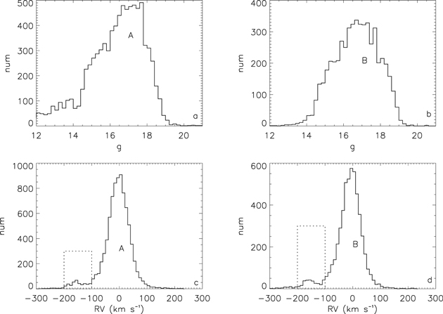
Figure 1. Panel (a): g magnitude distribution of stars in area A; panel (b): g magnitude distribution of stars in area B; panels (c), (d): RV distribution of stars in areas A and B. The rectangles of dotted lines indicate the overdensities in RV distribution.
Download figure:
Standard image High-resolution image3. Testing Substructures in Areas A and B
The bimodal RV distribution motivated us to look for similar substructures of proper motions and Vlos.
3.1. The Proper Motion Distributions
Figure 2 displays the procedure by which we identified substructure using proper motion in area A. The same procedure was used for area B. The top panel shows the proper motion distribution of stars in area A. There is an overdensity centered at the (0, −2) mas yr−1 position. Considering the streams are distant and most members are giants, we divided the sample into dwarfs and giants. Stars with log g < 3.5 were regarded as giants and others were assumed to be dwarfs. In the middle panel, the green pluses are giants. Evidently the overdensity is more prominent in the sample of giants. Thus, we conclude this overdensity is mostly composed of evolved stars, which indicates they are relatively distant. To determine the most likely member candidates in this substructure, we adopted the Density-Based Spatial Clustering of Applications with Noise (DBSCAN) algorithm (Ester et al. 1996), a well-known clustering algorithm, to identify cluster stars by  . DBSCAN is based on the density and has no particular bias that depends on the shape of a distribution of points. In this work, we set up the parameters eps = 0.20 and minPts = 30 manually and identified 173 sources in area A. In area B we set eps = 0.30 and minPts = 25 and identified 128 stars.
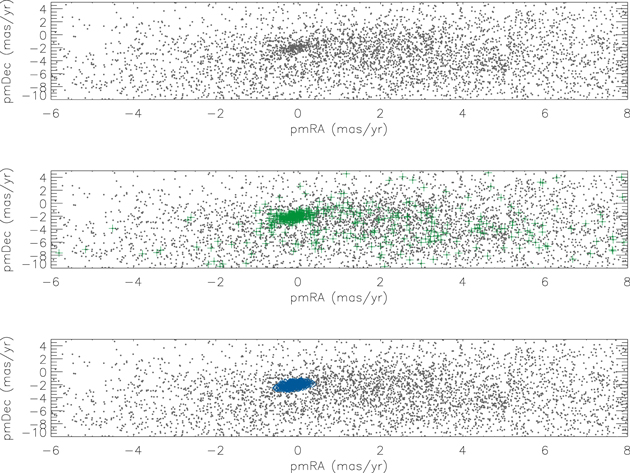
Figure 2. Proper motion distribution of area A. Top panel: proper motion distribution for all of the stars in area A. Middle panel: gray points represent all of the stars in area A, while green pluses represent giants in area A. Bottom panel: gray points are stars in area A. Blue diamonds are member candidates in the overdensity with the DBSCAN algorithm.
Download figure:
Standard image High-resolution image3.2. Overdensities in Vlos Distribution
Figure 3 shows the Vlos distribution of stars in areas A and B. Top panels and bottom panels show the Vlos distributions for both dwarfs and giants, respectively. In the bottom panel, we find very prominent peaks in the Vlos distribution for giants in both areas A and B.
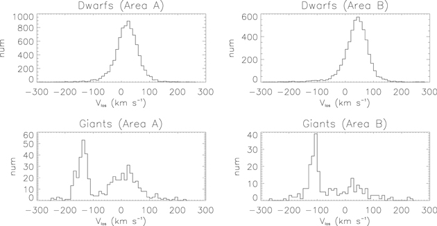
Figure 3. Overdensities in Vlos distributions of areas A and B. Top panels: Vlos distribution for dwarfs of areas A and B. Bottom panels: Vlos distribution for giants.
Download figure:
Standard image High-resolution image3.3. Identification of Member Candidates
The member candidates were initially identified by both proper motions and Vlos. For proper motions, the member candidates selected by DBSCAN algorithm as dwarfs were removed because they would be too nearby to be members of streams. Only giants with Vlos ranging in [−180, −110] km s−1 for area A and [−150, −90] km s−1 for area B are considered as candidates. Thus, with restrictions from the proper motions and Vlos, 220 stars as initial member candidates were determined. The distances implied by Gaia parallaxes for these 220 stars are all less than 10 kpc, indicating they are not accurate for a distant star. Thus, we adopted the photometry distance for these giants. The typical uncertainties of Teff, log g, [Fe/H], and [α/Fe] of these member candidates are 120 K, 0.4 dex, 0.25 dex, and 0.13 dex, respectively.
3.4. Connection with Known Substructures
Using high-precision photometry and spectroscopic digital sky surveys such as SDSS, APOGEE, RAVE, etc., has identified a number of substructures in the Milky Way. Except the Sgr stream, more substructures have been detected, such as the Orphan Stream, Monoceros Ring, Hercules–Aquila Cloud, Virgo Overdensity, etc. Because the LaCoSSPAr overlaps with the Sgr stream fields, we tentatively identified the overdensities detected above with this stream.
Figure 4 illustrates the possible connection between the Sgr stream and the substructures in areas A and B using spatial positions (panels (a)–(b)), proper motions (panels (c)–(d)), Vlos distribution (panels (e)–(f)), and distance to the Sun (panels (g)–(h)). The black points are particles in the LM10 model for the Sgr stream. The pink points are our stream candidates in two substructures. The left panels correspond the trailing arm of the Sgr stream, while the right panels shows the leading arm. The member candidates in both areas fit well with the orbits, proper motions, and Vlos of trailing arm. Thus, we conclude the substructures detected in areas A and B belong to the Sgr stream. However, in the distance to the Sun, some member candidates apparently lie outside of the trailing arm of the Sgr stream. They hypothesize some halo stars may be mixed in the member candidates. To exclude these possible contaminants, only 106 stars whose distance to the Sun is larger than 18 kpc were kept as the reliable members of those two substructures.
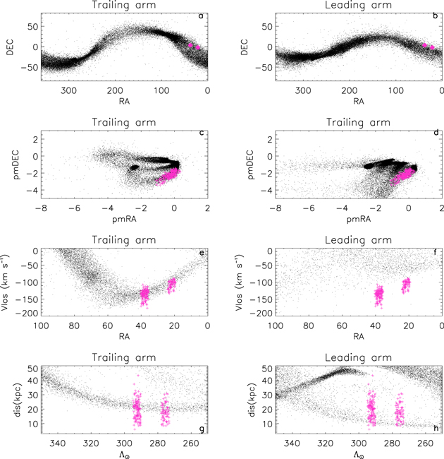
Figure 4. The spatial position, proper motion, Vlos, and distance to the Sun distribution in the trailing arm (left panels) and leading arm (right panels) of the Sgr stream from the LM10 model. Pink points are the member candidates in areas A and B.
Download figure:
Standard image High-resolution image4. Metallicity and α Abundance
The chemical properties of stream candidates are very important metrics since the stars retain the primordial abundance of the original molecular cloud. The abundance pattern of the member stars can be used to trace the formation and enrichment history of the progenitor cloud. Monaco et al. (2007) presented radial velocities for 67 stars belonging to the Sgr stream and iron along with α(Mg, Ca) abundances for 12 stars in the sample. The stream stars follow the same trend as Sgr main body stars in the [α/Fe] versus [Fe/H] plane. On average, the [Fe/H] of stars in this stream are metal-poor compared to stars in the main body.
It has been shown that the chemical abundance patterns of Sgr are unique. The metal-rich Sgr stars ([Fe/H] > −0.8) exhibit deficiencies in all chemical elements (expressed as [X/Fe]) relative to the MW (see, e.g., McWilliam et al. 2013; Hasselquist et al. 2017). Recent work confirms these abundance patterns extend to the Sgr tidal streams as well (Carlin et al. 2018). Carlin et al. (2018) analyzed [Fe/H] and [α/Fe] of 42 member stars of the Sgr stream both in the leading and trailing arms. They found the average [Fe/H] for the stream is lower than that of the Sgr core, and stars in the trailing and leading arms show systematic differences in [Fe/H].
Chou et al. (2010) presented high-resolution spectroscopic measurements of the abundances of the α-element titanium (Ti) and s-process elements yttrium (Y) and lanthanum (La) for 59 candidate M-giant members of the Sgr dSph + tidal tail system preselected on the basis of position and RV. The abundances of these stars show a different pattern from MW stars. The metallicity ranges from −1.4 to solar abundance. The overall [Ti/Fe], [Y/Fe], [La/Fe], and [La/Y] patterns with [Fe/H] of the Sgr stream plus Sgr core, for the most part, resemble those seen in the LMC and other dSphs, only shifted by Δ[Fe/H] +0.4 from the LMC and by +1 dex from the other dSphs.
Yang et al. (2019) found the trailing arm is on average more metal-rich than the leading arm. The α abundance of Sgr stars exhibits a similar trend to the Galactic halo stars at lower metallicity ([Fe/H] < −1.0 dex), but extends to lower [α/Fe] than Galactic disk stars at higher metallicity, which is close to the evolution pattern in dSphs.
4.1. [Fe/H] and [α/Fe] Distributions
Figure 5 provides the chemical abundance pattern of α elements. The top panel shows the normalized metallicity distribution of stars in the whole sample (black solid line), members in area A (blue solid line), and members in area B (green dashed line). The metallicity distribution in areas A and B are very consistent, but very different from the whole sample. The [Fe/H] distribution of the stream centers on ∼−0.9 and is lower than that of the whole sample. This indicates metal-poor stars dominate the stream. The bottom panel compares the α-abundance patterns of stream members and the halo field stars from the SAGA database (Suda et al. 2008).5 Other dwarf galaxies such as Carina, Ursa Minor, Draco, and Sculptor from the SAGA database are also displayed with colored open circles. Figure 5 shows that the [α/Fe] distribution among our stream candidates is very similar to that of Galactic field stars with [Fe/H] < −1.5. However, among stars with [Fe/H] > −1.0, [α/Fe] is lower among stream candidates compared to field stars with the same [Fe/H]. The most likely explanation is that α abundances are mainly enriched by the contribution of Type II supernovae, while iron peak elements are enriched by Type Ia supernovae (SNe Ia). The evolution of progenitor of stream would likely be slower than the Milky Way. SNe Ia begin to contribute at lower [Fe/H], leading to lower [α/Fe] than Galactic stars.
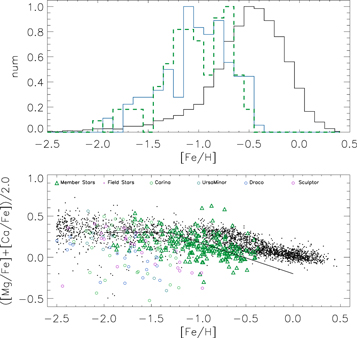
Figure 5. Metallicity distribution and α-abundance patterns for 106 member candidates. Top panel: metallicity distribution. Black solid line represents the normalized metallicity distribution for the whole sample. Blue solid line is metallicity distribution for member stars in area A, while green dashed line is for member stars in area B. Bottom panel: [α/Fe] vs. [Fe/H]. Black points are Galactic field stars from the SAGA database. Green diamonds represent the member candidates in our substructures. The colored open circles are some members of other dwarf galaxies from the SAGA database.
Download figure:
Standard image High-resolution imageMost dSphs have a different alpha-knee than the Milky Way, which locates at about [Fe/H] ∼ −1.0. We estimate the alpha-knee of the Sgr stream with [Fe/H] ∼ −1.1 ± 0.2 (solid line). This value is similar to the results of Carretta et al. (2010) and de Boer et al. (2015). This alpha-knee is also consistent with the star formation history (SFH) of massive dwarf galaxies.
4.2. Metallicity Gradient
Chou et al. (2007) investigated the variation of the metallicity distribution function (MDF) along the Sgr stream using M giants. The Sgr MDF was found to range from a median [Fe/H] ∼ −0.4 in the core to ∼−1.1 dex over the Sgr leading-arm length, representing ∼2.5–3.0 Gyr of dynamical (i.e., tidal stripping) age. Recently, Hayes et al. (2020) identified 166 Sgr stream members observed by APOGEE that also have Gaia DR2 astrometry. They found a mild chemical gradient along each arm.
Our stream candidates in areas A and B can be used to reaccess the local metallicity gradient in the Sgr stream. Figure 6 shows the [Fe/H] distribution among candidates in our sample. The top panel displays the [Fe/H] gradient along the orbit of the Sgr stream. The bottom panel shows the vertical [Fe/H] distribution. In the top panel, Λ⊙ represents the coordinate of the Sgr stream orbit. Filled points are four bins with different distances to the Sun in areas A and B. The color represents the mean metallicity in each bin. The distances range from 18 kpc to 30 kpc and the bin size is 3 kpc. Thus, our data suggest a very small [Fe/H] gradient along the orbit, which is consistent with that of previous research. The bottom panel shows the [Fe/H] gradient along the Z direction for stars in both A and B. The error bars are larger than the scatter. No evident metallicity gradients are found. Thus, along the stream orbit, we find a very small [Fe/H] gradient and no evident [Fe/H] gradient along the direction of vertical orbit among the member candidates in A and B. A more detailed investigation of the [Fe/H] gradients in the Sgr stream will require more data in much larger fields.
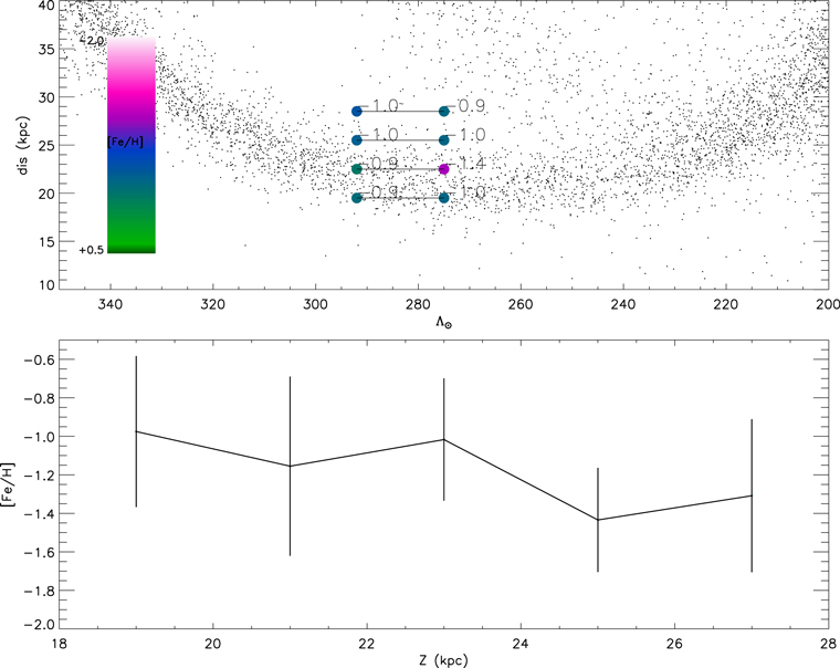
Figure 6. Top panel: [Fe/H] distribution in Λ⊙ vs. distance to the Sun. Λ⊙ represents the coordinate of the Sgr stream orbit. Filled points are four bins with different distances to the Sun in areas A and B. The color represents the mean metallicity in each bin. Bottom panel: [Fe/H] vs. absolute Z. Black solid line connects the points with different Z values. The error bar of each points are from the [Fe/H] scatter of each bin.
Download figure:
Standard image High-resolution image5. Conclusion
We identified two very prominent substructures in two areas of LaCoSSPAr A and B. With the proper motions and Vlos, we identified 220 initial candidate stream members. Using the LM10 model as a reference, two substructures were detected, which we propose are sections of the Sgr stream. As an additional filter on the preliminary sample, we excluded the candidates with distances to the Sun less than 18 kpc and obtained 106 likely member stars.
With [Fe/H] and [α/Fe] estimated from LAMOST spectra, the metallicity distribution of stars in the stream and total sample were analyzed. We estimated the alpha-knee at [Fe/H] ≈ −1.1 ± 0.2 dex, which is consistent with that from the literature. Finally, the [Fe/H] gradients were studied. [Fe/H] was found to vary slowly along the stream orbit between A and B.
The member stars in areas A and B provide two small windows of the Sgr stream. Although large progress has been made in the studies of the Sgr stream, more data in local fields along the orbit are needed to better characterize the entire stream and to constrain dynamical and chemical models.
This study is supported by the National Natural Science Foundation of China under grant Nos. 11988101, 11973048, 11927804, 11890694, 11625313, 11733006 and National Key R&D Program of China No. 2019YFA0405502. T.D.O. acknowledges support from the U.S. National Science Foundation grant AST-1910396 to Embry-Riddle Aeronautical University. This work is also supported by the Astronomical Big Data Joint Research Center, co-founded by the National Astronomical Observatories, Chinese Academy of Sciences and the Alibaba Cloud. Guoshoujing Telescope (the Large Sky Area Multi-Object Fiber Spectroscopic Telescope LAMOST) is a National Major Scientific Project built by the Chinese Academy of Sciences. Funding for the project has been provided by the National Development and Reform Commission. LAMOST is operated and managed by the National Astronomical Observatories, Chinese Academy of Sciences.