Abstract
Type Ia supernovae (SNe Ia) are more precise standardizable candles when measured in the near-infrared (NIR) than in the optical. With this motivation, from 2012 to 2017 we embarked on the RAISIN program with the Hubble Space Telescope (HST) to obtain rest-frame NIR light curves for a cosmologically distant sample of 37 SNe Ia (0.2 ≲ z ≲ 0.6) discovered by Pan-STARRS and the Dark Energy Survey. By comparing higher-z HST data with 42 SNe Ia at z < 0.1 observed in the NIR by the Carnegie Supernova Project, we construct a Hubble diagram from NIR observations (with only time of maximum light and some selection cuts from optical photometry) to pursue a unique avenue to constrain the dark energy equation-of-state parameter, w. We analyze the dependence of the full set of Hubble residuals on the SN Ia host galaxy mass and find Hubble residual steps of size ∼0.06-0.1 mag with 1.5σ−2.5σ significance depending on the method and step location used. Combining our NIR sample with cosmic microwave background constraints, we find 1 + w = −0.17 ± 0.12 (statistical + systematic errors). The largest systematic errors are the redshift-dependent SN selection biases and the properties of the NIR mass step. We also use these data to measure H0 = 75.9 ± 2.2 km s−1 Mpc−1 from stars with geometric distance calibration in the hosts of eight SNe Ia observed in the NIR versus H0 = 71.2 ± 3.8 km s−1 Mpc−1 using an inverse distance ladder approach tied to Planck. Using optical data, we find 1 + w = −0.10 ± 0.09, and with optical and NIR data combined, we find 1 + w = −0.06 ± 0.07; these shifts of up to ∼0.11 in w could point to inconsistency in the optical versus NIR SN models. There will be many opportunities to improve this NIR measurement and better understand systematic uncertainties through larger low-z samples, new light-curve models, calibration improvements, and eventually by building high-z samples from the Roman Space Telescope.
Original content from this work may be used under the terms of the Creative Commons Attribution 4.0 licence. Any further distribution of this work must maintain attribution to the author(s) and the title of the work, journal citation and DOI.
1. Introduction
After five decades of development as cosmological distance probes (Kirshner 2010), Type Ia supernovae (SNe Ia) are now mature tools for understanding cosmic acceleration (Riess et al. 1998; Perlmutter et al. 1999), and systematic errors will soon become the largest source of uncertainty in the parameters of cosmic expansion (Betoule et al. 2014; Riess et al.2016; Scolnic et al. 2018; Brout et al. 2019b; Jones et al. 2019; Brout et al. 2022). In the optical bands, where most SN Ia data have been obtained, substantial deviations from the behavior of a standard candle are reduced by correcting for the observed relations between light-curve shape and luminosity (Pskovskii 1977; Phillips 1993; Hamuy et al. 1996; Riess et al. 1996; Guy et al. 2007; Jha et al. 2007; Conley et al. 2008; Mandel et al. 2011; Burns et al. 2014), reddening by dust (Riess et al. 1996; Phillips et al. 1999; Burns et al. 2014; Thorp et al. 2021; Mandel et al. 2022), and the intrinsically redder color of less luminous SNe Ia (Tripp 1998; Mandel et al. 2017).
However, SNe Ia have been found to be more nearly standard candles in the near-infrared (NIR; wavelengths covered by the rest-frame zYJHK bands), and their light is also less sensitive to the effects of dust extinction at these wavelengths (Krisciunas et al. 2004, 2007; Wood-Vasey et al. 2008; Mandel et al. 2009, 2011; Barone-Nugent et al. 2012; Phillips 2012; Avelino et al. 2019; Mandel et al. 2022). This paper reports an attempt to realize these advantages in a cosmologically distant SN Ia sample.
At low redshift, significant samples of SNe Ia have been observed in the NIR by the Carnegie Supernova Project (CSP-I; Contreras et al. 2010; Stritzinger et al. 2011; Krisciunas et al. 2017) at Las Campanas Observatory in Chile and the CfA Supernova Survey (Wood-Vasey et al. 2008; Friedman et al. 2015) using PARITEL at the F. L. Whipple Observatory in Arizona. NIR SN Ia light curves from SweetSpot (Weyant et al. 2018) using the WIYN telescope at Kitt Peak National Observatory in Arizona have also been assembled, and additional data from CSP-II (Hsiao et al. 2019; Phillips et al. 2019), the VISTA Extragalactic Infrared Legacy Survey (VEILS), 25 UKIRT (Konchady et al. 2022), and the Hubble Space Telescope (HST) through the SIRAH program (HST-GO 15889; PI: Jha) are forthcoming.
Measurements of the dark energy equation-of-state parameter, w, require comparing low-z SNe to those at larger cosmological distances. Measurements of z > 0.1 SNe in the rest-frame NIR have only been obtained by Stanishev et al. (2018; four SNe) and Freedman et al. (2009). The only previous measurement of the dark energy equation of state using NIR data was the pioneering study of Freedman et al. (2009), who found w = −1.05 ± 0.13 (stat) ± 0.09 (sys) by comparing 21 low-z SNe to 35 high-z SNe using templates as red as the rest-frame I band with observations in YJ from the Magellan Baade telescope. This analysis was unable to apply a number of corrections that are now commonly included in cosmology analyses but were less well studied or entirely unknown at the time when Freedman et al. (2009) was published, including corrections for distance (Malmquist) biases and the dependence of Hubble residuals on host galaxy mass (Kelly et al. 2010; Lampeitl et al. 2010; Sullivan et al. 2010).
Though high-z NIR SN Ia observations are rare, the value of NIR data is clear from low-z analyses. Avelino et al. (2019) used CSP-I and CfA data to show in head-to-head comparisons of the same SNe that the scatter in the distances as measured in the infrared is smaller by 35% than distances determined from optical light curves. Studies such as Wood-Vasey et al. (2008), Mandel et al. (2009), Kattner et al. (2012), and Mandel et al. (2022) have also shown evidence that SNe at NIR wavelengths yield more precise distance measurements.
Low-z NIR data have recently been used to demonstrate a significant relationship between SN Ia distance residuals and the mass of the SN Ia host galaxy (Uddin et al. 2020; Ponder et al. 2021), which was originally discovered at optical wavelengths (Kelly et al. 2010; Lampeitl et al. 2010; Sullivan et al. 2010), although Johansson et al. (2021) found mildly conflicting results with no evidence for a mass step in the JH bands and ∼2σ evidence for a step in the Y band. Burns et al. (2018) and Dhawan et al. (2018) used NIR data to measure the Hubble constant, H0, using this new SN Ia wavelength range to provide additional evidence for tension between Cepheid+SN distance ladder measurements of H0 (e.g., Riess et al. 2021) and the cosmic microwave background (CMB; Planck Collaboration et al. 2020).
With the advent of the Nancy Grace Roman Space Telescope, developing the optimal ways to measure NIR distances at cosmological redshifts is now urgent. Although Roman will observe SNe Ia primarily at rest-frame optical wavelengths at maximum redshifts up to ≳2.5 (Hounsell et al. 2018), Roman SN Ia observations will be in the rest-frame NIR in the important regime at z ≲ 0.7, where baryon acoustic oscillation constraints will be limited by the cosmic volume (Weinberg et al. 2013).
Here we present NIR cosmological parameter measurements from the RAISIN survey. RAISIN (an anagram for “SNIA in the IR”) used 23 SNe Ia discovered in the Medium Deep Survey (MDS) of Pan-STARRS (Chambers et al. 2016) in Hawaii and another 23 discovered by the Dark Energy Survey (DES) at Cerro Tololo Inter-American Observatory in Chile (The Dark Energy Survey Collaboration 2005). We triggered Hubble Space Telescope observations of those objects with WFC3-IR using the F125W and F160W filters. After applying a number of well-motivated cuts to the data, we use 42 low-z SNe Ia from CSP-I (hereafter CSP) and 37 high-z (z > 0.2) SNe Ia from RAISIN to measure w.
In this work, we pursue an “NIR-only” cosmological analysis that uses a different wavelength range than previous cosmological analyses with SNe and will have reduced systematic uncertainties due to dust. An optimal combination of optical+NIR data would yield the most precise cosmological constraints, but we show that an NIR-only analysis offers additional independent distance information. Throughout this paper we enumerate areas that will be improved to shrink these errors in future NIR studies and compare our results to a combined optical+NIR measurement.
In Section 2 we describe the RAISIN data, including survey properties, classifications, and photometric measurements. In Section 3 we describe our analysis method. In Section 4 we present our baseline cosmological results, and in Section 5 we discuss additional analysis variants and measure the correlation of Hubble residuals with host galaxy mass. In Section 6 we discuss the implications of our results for future missions such as the Roman Space Telescope. In Section 7 we conclude.
2. The RAISIN Sample
2.1. Overview and Strategy
The RAISIN program was carried out in cycle 20 through HST-GO 13046 (hereafter RAISIN1; PI: Kirshner) and cycle 23 through HST-GO 14216 (hereafter RAISIN2; PI: Kirshner). RAISIN1 followed 23 spectroscopically classified SNe from the Pan-STARRS MDS (Chambers et al. 2016), and RAISIN2 followed 23 spectroscopically classified SNe from DES (The Dark Energy Survey Collaboration 2005). RAISIN1 observed SNe in the redshift range of 0.22 ≤ z ≤ 0.50 and RAISIN2 observed SNe at 0.35 ≤ z ≤ 0.61 to observe at redshifts where the available HST filters overlap with the rest-frame YJH filters to minimize K-correction uncertainties. The median redshifts of PS1 and DES SNe aligned well with these targeted redshift ranges.
Due to occasional poor weather during PS1 and DES observing seasons and the need for HST template imaging after each SN had faded, RAISIN observations for each program extended over a period of 1.5−2 yr; RAISIN1 observations were taken from 2012 October 29 to 2014 June 17, and RAISIN2 observations occurred from 2015 September 28 to 2017 November 21.
To select RAISIN candidates, we identified Pan-STARRS and DES SNe that were likely to be SNe Ia discovered before maximum light. These candidates were then classified spectroscopically; classifications for MDS and DES SNe were carried out either by the RAISIN team in collaboration with the survey teams or by the MDS or DES teams themselves. For RAISIN1, we selected candidates that had been discovered by the Pan-STARRS team and were consistent with having a light-curve phase approximately 5−10 days before maximum light. For RAISIN2, we similarly selected candidates based on their apparent light-curve phase and additionally required that the photometric redshifts of their host galaxies were consistent with the target redshift range of ∼0.5 ± 0.1.
Most classifications were from Magellan (16 SNe) and Gemini South (13 SNe), with additional classifications from Gemini North (four SNe), the MMT (six SNe), the AAT (three SNe), and Keck (three SNe). Each classification was determined using the SN IDentification software (SNID; Blondin & Tonry 2007), which uses cross-correlation matching to template SNe to yield SN types, light-curve phases, and redshifts. Representative spectra for RAISIN targets are shown in Figure 1. Spectroscopically classified SNe Ia with rising light curves within the target redshift range were submitted to STScI for scheduling as nondisruptive targets of opportunity on HST. To improve the distance measurement, two additional epochs were obtained for each SN after the initial HST observation, spaced by approximately 5 rest-frame days. Template images for each SN were taken at least 6 months after the initial observations, with the exception of a single SN for which no template was needed because it was located in a region with no apparent galaxy light.
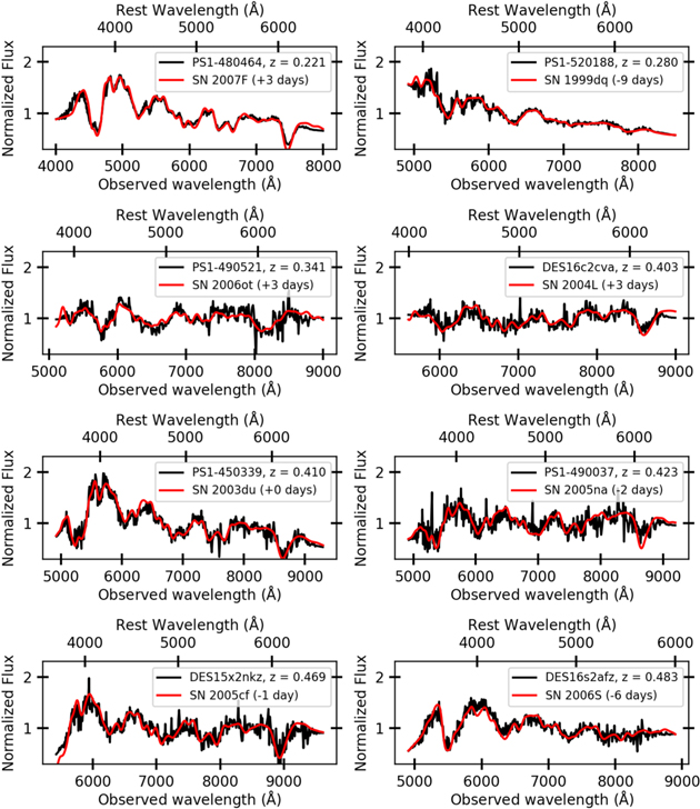
Figure 1. Representative classification spectra for RAISIN SNe (black) with the best template matches from SNID (red). Though the template match to PS1-490521 (SN 2006ot) is a peculiar Ia, the SNID matches to normal SNe Ia are also excellent.
Download figure:
Standard image High-resolution image2.2. Ground-based Data and Photometry
2.2.1. The Pan-STARRS Medium Deep Survey
The Pan-STARRS MDS, the source of RAISIN1 SNe, observed 70 deg2 in griz filters over approximately 4 yr, with gr, i, and then z observations on successive nights. MDS also observed in the y filter, primarily during bright time, but the signal-to-noise ratio (S/N) of y-band observations for objects in our targeted redshift range was too low to be of use for SN Ia cosmology. Approximately 5200 SNe were discovered across the 4 yr of the MDS, with over 3000 host galaxy redshifts measured (Jones et al. 2017). A total of 520 SNe were spectroscopically classified during the survey, with ∼350 of these being SNe Ia and having a median redshift of ∼0.35 (Scolnic et al. 2018). Cosmological parameter measurements from these data are presented in Scolnic et al. (2018) for the spectroscopically classified sample and in Jones et al. (2018b) for the full sample. Further details regarding the MDS are given in Chambers et al. (2016).
The optical photometry for RAISIN1 comes from the Pantheon cosmological analysis (Scolnic et al. 2018), with the exception of five SNe that were not included in Scolnic et al. (2018). 26 Light curves of those five SNe were published by Villar et al. (2020) and are included in the data release that accompanies this paper. Pan-STARRS SN photometry is from Photpipe (Rest et al. 2005), with details specific to the MDS given in Rest et al. (2014) and Scolnic et al. (2018). In brief, MDS images are astrometrically aligned, and their zero-points are measured using the PS1 catalog. PS1 zero-points have been calibrated to a 3 mmag relative precision across the sky (Schlafly et al. 2012; Scolnic et al. 2015; Brout et al. 2021). Single-season, inverse-variance-weighted template image stacks are then convolved and subtracted from the nightly images, and SNe are discovered and their light curves subsequently measured by performing DAOPHOT forced photometry on the resulting difference images (Stetson 1987).
2.2.2. The Dark Energy Survey
DES observed in griz filters over 27 deg2 with a cadence of approximately once per week. These 27 deg2 were split into eight 2.7 deg2 “shallow” fields, with depths of ∼23.5 mag, and two “deep” fields, with depths of ∼24.5 mag. DES spectroscopically classified 251 SNe Ia at redshifts 0.02 < z < 0.85 (Abbott et al. 2018). After sample cuts, their 3 yr spectroscopic sample includes 207 SNe Ia at a median redshift of z = 0.36. Cosmological parameter measurements from the DES spectroscopic sample are given in Abbott et al. (2018), with additional publications describing the calibration (Burke et al. 2018; Lasker et al. 2019), primarily based on observations of the CALSPEC standard star C26202, bias corrections (Kessler et al. 2019), photometry (Brout et al. 2019a), spectroscopic classification (Smith et al. 2020), and systematic uncertainties (Brout et al. 2019b) of these data.
For RAISIN2, DES SN discovery uses a difference imaging procedure similar to the MDS, but final optical photometry is carried out using the scene-modeling algorithm presented in Brout et al. (2019a). Scene modeling (Holtzman et al. 2008) uses imaging data to build a pixel-based model of the galaxy+SN that is convolved with each night’s measured point-spread function (PSF) model. The amplitude of the SN is allowed to vary epoch to epoch, while the galaxy brightness is fixed. The robustness of the algorithm has been tested with artificial sources and recovers fluxes to an accuracy of 3 mmag.
2.2.3. The Carnegie Supernova Project
There are two sources of well-sampled low-z NIR SN Ia data, the CfA and CSP samples (Friedman et al. 2015; Krisciunas et al. 2017). These were combined to yield a sample of 89 low-z, NIR-observed SNe in Avelino et al. (2019). However, most CfA SNe either are at redshifts where the effect of peculiar flows dominates the distance uncertainty (z ≲ 0.01) or lack data prior to maximum light, which makes the determination of the time of maximum light uncertain and increases distance uncertainties. Therefore, we restrict ourselves to the CSP data for the low-z SN sample used in this work, although the CfA data remain extremely useful for training SN standardization models in the NIR. The release of CSP-II data in the near future will add an additional 125 SNe with NIR light curves and 90 SNe with NIR spectra (Hsiao et al. 2019; Phillips et al. 2019).
CSP uses DAOPHOT (Stetson 1987) to measure natural-system photometry on SN images after a template image, taken once the SN light has faded, has been subtracted. CSP images are calibrated with respect to primary standards BD +17°4708 (optical bandpasses) and Vega (NIR), with additional details given in Krisciunas et al. (2017).
2.2.4. Spectroscopic Classifications and Redshifts
Spectroscopic classifications and SN redshifts for each RAISIN SN were determined using SNID (Blondin & Tonry 2007). SNID determines a classification quality through a combination of the overlap between the observed spectrum and a template spectrum (lap) and the height of the cross-correlation peak (r). We ensure that the best template match has an rlap > 5, indicating a good match, and that the top three spectroscopic matches are all normal SNe Ia. For SN PS1-520107, the classification was unclear, so we remove this SN from our sample. For SN PS1-490521 the best-matched spectrum was to the peculiar SN Ia 2006ot, but, as discussed in Section 3.4, we choose to include 06bt- and 06ot-like SNe in our cosmology analysis, as they cannot be reliably classified (or ruled out) from noisier high-z spectra.
The PS1 and DES teams measured host galaxy redshifts for these objects using cross-correlation matches to galaxy templates. For PS1, redshifts were estimated using the rvsao package (Kurtz & Mink 1998), and for DES the Marz package was used (Hinton et al. 2016).
For CSP classifications and redshifts, see Krisciunas et al. (2017) and references therein. SN classifications were measured from SNID, as well as SN redshifts. As discussed in Krisciunas et al. (2017), all CSP SNe have host galaxy redshifts, and nearly all of these are measured from the NASA/IPAC Extragalactic Database (NED 27 ). We also use updated group redshifts from the Pantheon+ analysis (Scolnic et al. 2021) for SN 2005al and SN 2009ab, which differ significantly from the values in the latest CSP data release.
2.3. HST Data and Photometry
The HST data for RAISIN1 SNe were taken with three epochs each of F125W (approximately the J band) and F160W (approximately the H band). For RAISIN2 SNe, only the F160W band was used for most SNe; five RAISIN2 SNe included data in both filters. Figure 2 illustrates the rest-frame wavelengths probed by the HST data as a function of redshift.
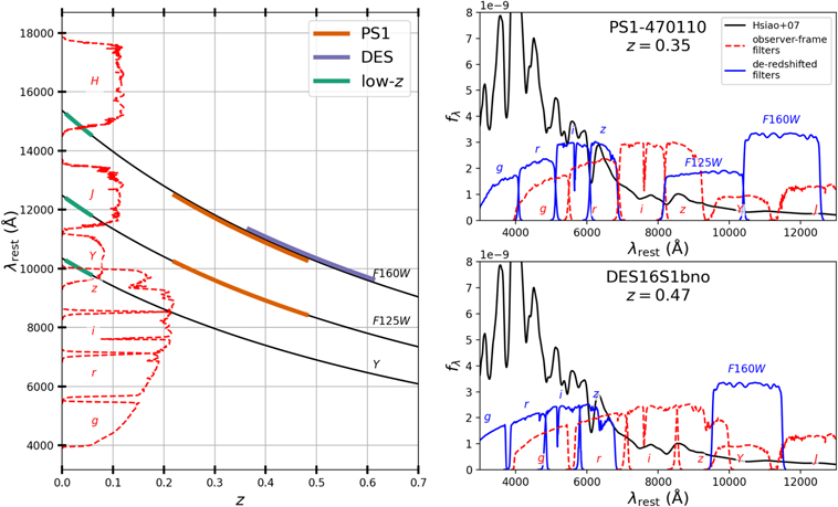
Figure 2. Rest-frame wavelengths probed by RAISIN observations as a function of redshift. Left: rest-frame wavelengths corresponding to the observer-frame Y, F125W (HST's J band), and F160W (HST's H band) as a function of redshift, with the low-z, RAISIN1 (PS1) and RAISIN2 (DES) redshift ranges highlighted. The shapes of grizYJH filter throughputs (red; arbitrary units) are shown for illustration. Right: de-redshifted (solid blue) and observer-frame (dashed red) filters for the median-redshift RAISIN1 (top) and RAISIN2 (bottom) SNe. The Hsiao et al. (2007) model (black) is shown for illustration.
Download figure:
Standard image High-resolution imageThe first HST observations occurred at a median of 12.2 observer-frame days relative to B-band maximum light for RAISIN1 (+9.2 rest-frame days) and 13.9 observer-frame days (+9.5 rest-frame days) for RAISIN2 owing to the time required for SN discovery, classification, and the latency in the HST scheduling. The median S/N is 12.5 for RAISIN1 and 12.9 for RAISIN2, with template observations taken at an average of 189 days after the first SN detection. See Appendix A for a discussion of how we correct for a small amount of late-time SN flux in some template images.
Examples of RAISIN observations are shown in Figure 3. Optical photometry and spectra of these SNe are provided in the online data release accompanying this paper to allow these measurements to be of use in future NIR analyses such as SIRAH (HST-GO 15889).
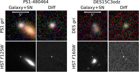
Figure 3. Stamp images of RAISIN SNe from Pan-STARRS (left) and DES (right) with gri images (top) and RAISIN images from HST (bottom). The SN location is centered in each image.
Download figure:
Standard image High-resolution imageOur team measured photometry from the RAISIN images according to the following steps:
- 1.For each epoch, FLT images, which are images that have been bias-subtracted, dark-subtracted, and flat-fielded, are drizzled 28 together, and the final (template) epoch is subtracted.
- 2.We then measured SN centroids from the difference images and performed 0
4 aperture photometry on the difference images with aperture corrections from HST. We verified these aperture corrections using drizzled images of the CALSPEC standard star P330E.
- 3.Using artificial stars injected into the data frames, we corrected the resulting measurements and uncertainties for host galaxy noise.
- 4.We calibrated the data using publicly available zero-points that were measured from observations of four white dwarf standards (GD153, G191B2B, GD71, GRW+70D5824) and the G-type star P330E. 29
We describe these steps in additional detail in Appendix A. Coordinates of the RAISIN SNe and the final RAISIN photometry are given in Appendix B.
3. Analysis
In this section, we describe the NIR light-curve models we used (Section 3.1), present our method for distance measurements (Section 3.2), create a dispersion model to measure distance-dependent biases (Section 3.3), apply sample selection cuts (Section 3.4), measure the dependence of distance on host galaxy mass (Section 3.6), and estimate each source of systematic uncertainty in our NIR measurement of w (Section 3.7). Our cosmological parameter measurements are then presented in Section 4.
3.1. NIR Light-curve Models
SN Ia standardization models rarely make use of the NIR owing to the small number of well-calibrated, high-cadence NIR light curves. In the past decade, only the SALT2 (Guy et al. 2007, 2010) and SiFTO (Conley et al. 2008) light-curve fitters have been used for measurements of w, with SALT2 being by far the most common model. SALT2, however, extends only to a central filter wavelength of approximately 7000 Å, with the recently developed SALT3 model (Kenworthy et al. 2021) now extending this wavelength to 8700 Å to include the rest-frame z band.
However, there are now two well-vetted light-curve models extending to the NIR: the SNooPy model (Burns et al. 2011, 2014) and the BayeSN model (Thorp et al. 2021; Mandel et al. 2022). SNooPy benefits from over a decade of use by the community and includes light-curve templates for the uBVgriYJH bands that have been trained using well-calibrated CSP light curves. BayeSN is a hierarchical Bayesian spectral energy distribution (SED) model for SNe Ia (BayeSN) that models time-dependent optical−NIR (to 1.8 μm) SN Ia SEDs as a combination of physically distinct intrinsic spectral components and host galaxy dust effects. By having an SED-based model continuous in both time and wavelength, BayeSN removes the need to compare high-redshift photometric data to an approximate rest-frame filter and effectively allows a K-correction that varies with light-curve stretch. At the same time, BayeSN has yet to be integrated in publicly available tools like SNANA (Kessler et al. 2010), so the simulation of distance-dependent biases for a cosmology analysis is not yet feasible.
Though we incorporate both SNooPy and BayeSN in our analysis, we use SNooPy as our baseline method owing to the greater ease of determining distance biases and because BayeSN was under development during the time when much of this analysis was carried out. The advantages of BayeSN’s statistical framework are somewhat mitigated owing to the limited number of NIR observational epochs in the RAISIN data. Still, we find good consistency between the distance measurements from these two models, as demonstrated in Section 5.2.1; we plan to use BayeSN in a future optical+NIR analysis of these data.
3.1.1. SNooPy Model Philosophy
The SNooPy model philosophy assumes that the observed variation in SN colors is caused by extinction in the SN host galaxy but allows the selective-to-total extinction ratio RV to be specified by the user—the nominal method in this analysis—or fit by the data. We also allow SNooPy to fit negative extinctions for a more agnostic treatment of SN color; SNooPy assumes the luminosity versus color relationship to be linear with no minimum value (the same philosophy as the Tripp relation; Tripp 1998). This effectively means that RV should be interpreted as a luminosity versus color trend in this work, rather than a physical dust law.
SNooPy also includes options to correct for the dependence of SN luminosity on light-curve shape. We adopted the “EBV_model2,” which uses the sBV parameter to determine the relation between SN light-curve shape and luminosity (Burns et al. 2018). The sBV parameter is a stretch parameter that is insensitive to extinction because it takes advantage of the fact that the delay between time of maximum light and the time of reddest color is insensitive to reddening (Lira et al. 1998). To enable easier determinations of distance biases and systematic uncertainties in later stages of the analysis, we incorporated this SNooPy model into the SNANA software (Section 3.5; Kessler et al. 2010) and used the SNooPy iYJH templates generated from low-z CSP data to fit our NIR data and measure distances. Example RAISIN light curves with SNooPy fits are shown in Figure 4.
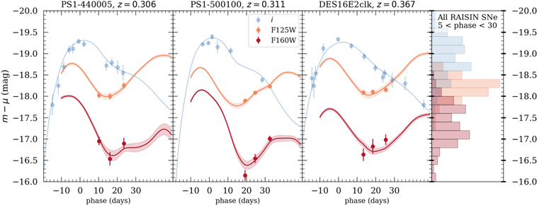
Figure 4. Examples of RAISIN SN light curves. Apparent magnitude minus distance modulus (a proxy for absolute magnitude) versus phase is shown for three RAISIN SNe with observations in i (PS1 or DES), F125W, and F160W. Solid lines show the SNooPy model fit to the data. The optical bands, including i, are used to estimate the time of maximum light, while the HST NIR bands are used to measure the distance (we allow sBV fitting to show the best-fit NIR model in this example). Histograms with approximate absolute magnitude distributions for all RAISIN SNe are shown on the right after applying the sample selection cuts discussed in Section 3.4.
Download figure:
Standard image High-resolution image3.2. Distance Measurement Method
Because RAISIN NIR light curves include just three post-maximum light epochs per SN, we are unable to make robust shape and color corrections or determine the time of maximum light from NIR data alone; we find a Hubble residual rms of 0.24 mag when fitting AV and 0.28 mag when fitting sBV from NIR-only RAISIN data (in Appendix C, we will use simulations to confirm that larger rms values are expected given the small number of post-maximum light epochs per SN).
Therefore, our nominal distance measurement approach is to use the SNooPy model to fit only the NIR SN amplitude; we use optical data to determine the time of maximum light and fix the SN shape and color to a nominal value. 30 This approach yields a Hubble residual rms of 0.18 mag.
We relax either the NIR-only aspect of this analysis or the nominal approach of fitting only the amplitude of the NIR data—i.e., not fitting sBV or AV —in several places in this analysis as described below:
- 1.Selection cuts. Optical data are used to make sample selection cuts to remove SNe with high values of E(B − V), which cannot be estimated from NIR data alone. This is discussed in Section 3.4.
- 2.Time of maximum light. Because we do not have NIR data near maximum light in the high-z sample, we must use optical data to constrain the phase of the SN observations.
- 3.Scatter model. SNe Ia were discovered and spectroscopically classified at optical wavelengths, so we determine the consequence of these selection effects on our sample. To estimate distance-dependent selection effects for the SNooPy model, we use optical+NIR CSP data to estimate the covariance matrix of the distance residuals after estimating and correcting for sBV and AV . This is described below in Section 3.3.
- 4.Bias corrections: To determine and correct for the redshift dependence of the intrinsic populations of sBV , we fit sBV using the NIR data. Though the resulting Hubble residual scatter increases, as discussed above, this is a useful tool to compare data distributions of sBV to simulated distributions of sBV . This is described in Appendix C.
- 5.Wavelength dependence of the mass step. In Section 5.1, we compare estimates of the host galaxy mass step between optical and NIR data in a self-consistent manner that accounts for the correlation between sBV and galaxy mass. Therefore, in this section we will correct the NIR Hubble residuals for their dependence on the optical+NIR-measured sBV parameter. We use both the SNooPy derived sBV −NIR luminosity correlation and the directly measured dependence of our NIR Hubble residuals on sBV . An sBV -corrected mass step is not used for cosmological parameter estimation but only to investigate the physics and wavelength dependence of the mass step.
- 6.Comparing to optical and optical+NIR measurements of w. In Section 4.1, we compare the baseline results to results that fit the SNooPy model to optical and optical+NIR data.
3.3. Dispersion Model and Distance Biases
Because we compare SNe Ia across a large span of redshift, we must determine distance-dependent biases, which are caused by the increased likelihood of discovering higher-luminosity SNe at larger redshifts in magnitude-limited surveys; these can be up to ∼5% in distance for the PS1 and DES samples (Scolnic et al. 2018; Brout et al. 2019b). To determine these biases, we build a dispersion covariance matrix from the optical to NIR to understand the ways in which optical SN Ia selection effects—which are caused by PS1 and DES selection criteria—affect distances measured in the NIR.
Because there has been no measurement of the covariance in magnitude between different SNooPy bands, we estimated this model from the low-z CSP data in our sample. To generate this model, we use low-z SNe at 0.015 < z < 0.1 to ensure that the results are minimally dependent on cosmological parameters while also mitigating the effect of peculiar velocity uncertainties at z < 0.015 (Peterson et al. 2021).
We then simultaneously fit the SNooPy model to all the optical and NIR bands in the low-z CSP sample to estimate the time of maximum light, sBV , and AV for each SN. Keeping these parameters fixed, we then fit the low-z data with the SNooPy model for each of the BVgriYJH bands individually. We use the resulting Hubble residuals in each band to generate a band-to-band covariance matrix that can be used to generate large Monte Carlo simulations and determine wavelength-dependent distance biases. We note that the additional distance scatter predicted from a peculiar velocity uncertainty of 250 km s−1 (Scolnic et al. 2018) is smaller than the scatter observed in each band at the median redshift z = 0.023, and we find that the observed optical-to-NIR covariances are very similar when restricting the sample to z > 0.025 or z > 0.03.
The resulting covariance matrix is shown in Figure 5 and is now included in the public SNANA software. 31 We find similar dispersion measurements in most bands, with values ranging from ∼0.116 to 0.136 mag; the maximum dispersion is in the H band, and the minimum is in Y, but the band-to-band differences are not highly significant in this sample. Covariance is on the order of ∼0.015 mag2 between neighboring optical bands (correlations of ≳0.95) and ∼0.010 mag2 between NIR-to-NIR and optical-to-NIR bands (correlations of ∼0.78−0.86). These correlations can be understood as the correlation between Hubble residuals measured using one band at a time. Slightly higher correlations are found when we examine the Uddin et al. (2020) data, which might be due to the exclusion of fast-declining, red, and low-z SNe in the present analysis. NIR-derived distances in our sample are well correlated with optical distances—implying a significant wavelength-independent component of SN Hubble residual scatter—but are less correlated with optical bands than optical bands are with each other, implying that NIR data contain additional information useful for constraining SN Ia distances.
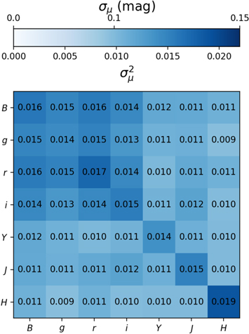
Figure 5. Optical-to-NIR covariance matrix for the SNooPy model computed from CSP data (similar to Figure 6 of Mandel et al. 2011), with covariance values labeled and the top axis of the color bar indicating the uncertainties on the diagonal in each band. After shape and color correction, we found the maximum dispersion to be ∼0.15 mag in the optical bands and the minimum to be ∼0.12 mag in the Y band.
Download figure:
Standard image High-resolution image3.4. Sample Selection Cuts
Next, we apply selection cuts to our sample to ensure that each SN has well-measured photometry and distances. First, as discussed in Appendix A.1, we remove five SNe with host galaxy noise contributions that add greater than 0.1 mag to the photometric errors, based on an injected star analysis, as these are indications of subtraction residuals. Due to PSF variation caused by the breathing of HST, it is difficult to have clean subtractions on galaxies that are bright relative to the SN; this is because even few-percent variations in the PSF when multiplied by a bright galaxy core can cause large residuals relative to the brightness of the SN. This PSF variation will unavoidably bias our sample against SNe in high surface brightness environments, making it even more important to better characterize the SN–host galaxy environment correlation. We visually inspect each difference image to ensure that the remaining SNe appear to have high-quality subtractions. We also remove SN PS1-520107, which has an unclear spectroscopic classification. We note that SN 2006bt is peculiar (Foley et al. 2010), but we chose to include it for consistency across the redshift range, as similar events would be impossible to identify and exclude in our high-z sample given the noisier spectra at those redshifts. However, SN 2006bt subsequently fails Chauvenet’s criterion (see below). We further remove SNe that lack either optical or NIR data before maximum light, as this makes it impossible to accurately determine the phase of a given observation. We also ensure that pre-maximum light data exist both before and after removing >10σ SNooPy light-curve fit outliers from the data; if an SN had a misidentified time of maximum light, we found that an SN could appear to have pre-maximum light data when in reality it did not, but this issue was fixed once we removed outlying data points from the fit.
Next, we remove SNe measured to have E(B − V) >0.3 mag from optical data. Though only a single SN in our sample fails this cut, these SNe could in principle cause large outliers on our NIR-only Hubble diagram given that we perform light-curve fits with fixed AV . High-AV SNe could also have some sensitivity to differences in RV that are difficult to measure owing to the extrinsic/intrinsic degeneracy in SN colors (e.g., Mandel et al. 2022). We also remove SNe with extreme values of the sBV parameter that are not well represented in the SNooPy training sample. These include sBV > 1.18 and sBV < 0.75, values for which SNooPy is not well trained. Cutting at sBV > 0.75 also excludes 91bg-like and transitional SNe Ia (see Burns et al. 2014; Gall et al. 2018), which removes SNe that would be poorly standardized by our baseline method that does not fit for sBV . At sBV > 1.18 in particular, only a single high-stretch SN is included in the SNooPy model training. SNe with sBV measurement uncertainties >0.2 are also removed, as we cannot reliably estimate whether they pass cuts. Finally, two SNe—SN 2006bt and DES15C1nhv—fail Chauvenet’s criterion as 2.8σ and 3.1σ outliers on the Hubble diagram. A sample of 38 objects (the high-z sample) is expected to have just 0.07 3.1σ (or greater) outliers on average, and a sample with 44 objects (the CSP sample) is expected to have just 0.2 >2.8σ outliers; both numbers are below the Chauvenet threshold of 0.5. We treat the low- and high-z distributions differently in this calculation, as they have substantially different photometric data coverage and scatter (Section 5.2.2).
The full set of distances, light-curve parameter measurements (using optical data), and cuts on those data for both the low-z and RAISIN samples are given in Appendix E. For each subsample, selection cuts are summarized in Table 1.
3.5. Simulations and Bias Corrections
Using the dispersion model from Section 3.3, we use the SNANA (Kessler et al. 2010) simulation framework to generate realizations of each subsample in this analysis (CSP, RAISIN1, and RAISIN2). SNANA is the “industry standard” tool for accurately simulating large SN Ia samples for cosmological parameter measurements, and for this reason both the MDS and DES teams have already developed sophisticated SNANA simulations of their surveys that yield accurate realizations of their survey data. SNANA includes sky noise, survey zero-points, survey cadences, host galaxy properties, realistic shape and color distributions for the SN population, and the quantitative criteria that were used to trigger follow-up observations.
These simulations are presented in Appendix C. In brief, we based our simulations on preexisting CSP (Kessler et al. 2019), PS1 (Scolnic et al. 2018), and DES (Kessler et al. 2019) simulations, but we applied them to a SNooPy model that we implemented within the SNANA framework (Figure 6). We then estimated intrinsic population distributions of the sBV values using the aggregate NIR data, and although NIR data are only weakly dependent on AV , we simulate a nominal exponential AV scale of τ = 0.2 mag and vary this scale length in our systematic error budget. This exponential scale is well matched to our measurements from optical observations, from which we estimate τ ≃ 0.15−0.18 mag; preliminary optical+NIR analysis of the RAISIN sample from BayeSN also gives τ = 0.21 ± 0.04.
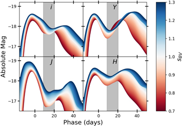
Figure 6. SNooPy model iYJH light curves as implemented in SNANA and as a function of the color-stretch parameter, sBV . The rest-frame Y-band model in particular has very little sensitivity to sBV at the epochs of the RAISIN data. The phase range within which 68% of RAISIN observations fall are shown in gray bands (for CSP the 68% range covers phases from ∼−3 to 40 days).
Download figure:
Standard image High-resolution imageThe simulations then give the distance bias: the average difference between simulated and measured distance as a function of redshift, shown in Figure 7. We correct the measured distances for the average bias at each SN redshift. The predicted optical distance biases have similar sizes to bias corrections generated for the Pantheon analysis (Scolnic et al. 2018) using the Guy et al. (2010) optical scatter model and the SALT2 standardization model. The NIR bias corrections are dominated by the difference in mean stretch and AV between the low- and high-z samples. The uncertainties on the differences in these distributions are used to determine systematic uncertainties on the bias corrections.
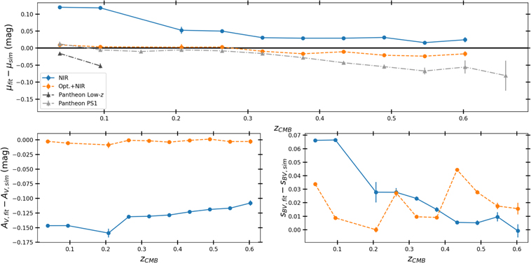
Figure 7. Distance biases (top), AV biases (bottom left), and sBV biases (bottom right) as a function of redshift. Results are shown for both the NIR-only light-curve fits (blue), which assume zero reddening and sBV = 1.0, and the optical+NIR fits (orange), which include AV and sBV as free parameters. Predicted low-z (black triangles) and PS1 (gray triangles) distance biases from Pantheon are also shown in the top panel. Some bin-to-bin fluctuation in the bias corrections as a function of redshift is caused by simulating SNe at only the exact redshifts of RAISIN objects for a smaller, more computationally efficient simulation.
Download figure:
Standard image High-resolution image3.6. Host Galaxy Mass Dependence
The step-like dependence of SN Hubble residuals on host galaxy mass has been well established (Kelly et al. 2010; Lampeitl et al. 2010; Sullivan et al. 2010), and recently there have been reported—but somewhat conflicting—detections of the host mass step in the NIR (Uddin et al. 2020; Johansson et al. 2021; Ponder et al. 2021). Constraining the wavelength dependence of the mass step could help to distinguish among theories for the origin of the step, e.g., dust properties (Brout & Scolnic 2021) versus progenitor metallicity (Rose et al. 2021b). We attempt to measure and correct for a host galaxy mass step in the RAISIN data. We measure host galaxy masses ourselves to ensure consistency across the sample using a procedure described in Appendix D. We simultaneously estimate the mass step and the average Hubble residual in three redshift bins to ensure that our measurement is independent of cosmological parameters. The resulting masses are shown in Figure 8.
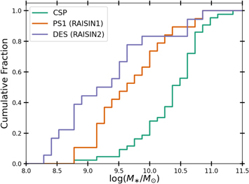
Figure 8. Cumulative fraction of SNe as a function of host galaxy mass for CSP and RAISIN SNe. CSP SNe are found in significantly more massive host galaxies.
Download figure:
Standard image High-resolution image3.7. Systematic Uncertainties
We treat systematic uncertainties in much the same way as previous cosmological analyses (e.g., Scolnic et al. 2018; Brout et al. 2019b; Jones et al. 2019): we determine 1σ uncertainties in data and analysis parameters (e.g., peculiar velocities, Milky Way (MW) reddening, calibration, and bias corrections), apply each systematic to the data or analysis, and construct a covariance matrix of the distances resulting from each analysis choice or data modification. The systematic uncertainty covariance matrix is then added to the (diagonal-only) statistical covariance matrix. The systematic uncertainty covariance matrix is given by

for a given set of systematics Sn
applied to each light curve or distance measurement. For the nth systematic,  is the change in distance after applying systematic Sn
to an SN at redshift zj
. The size of each systematic uncertainty is given by σ(Sn
).
is the change in distance after applying systematic Sn
to an SN at redshift zj
. The size of each systematic uncertainty is given by σ(Sn
).
Details about individual systematic uncertainties are given below. Compared to previous analyses, our choice of the SNooPy model and the limited sample size allows us to omit a few second-order systematic uncertainties, including redshift evolution in nuisance parameters and redshift evolution of the host galaxy mass step. We also do not include the choice of SN Ia dispersion model as a systematic uncertainty because we have constrained this directly from the low-z Hubble diagram itself. We are therefore not subject to the G10/C11 scatter model degeneracy that causes significant uncertainties in optical-only analyses (e.g., Brout et al. 2019b). The redshift dependence of a subset of our systematic uncertainties is shown in Figure 9.
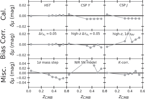
Figure 9. Selected systematic shifts in distance modulus as a function of redshift for this analysis, grouped into calibration systematics (top), bias correction systematics (middle), and other systematics (bottom). The systematics shown in the middle panel are a shift in the scale length of the AV distribution (left), a shift in the scale length of the AV distribution for the high-z data only (middle), and 1σ shifts in the high-z stretch distribution parameters (right). The systematics shown in the bottom panel are due to the uncertainty in the size of the mass step (left), the SNooPy model (middle), and K-correction uncertainties (right). The weighted average of each distance vector is subtracted to show relative low- to high-z differences, even if the systematic only changes the distances in one part of the redshift range. For visualization purposes, only bins with at least three SNe are shown to reduce noise while illustrating z-dependent trends.
Download figure:
Standard image High-resolution image3.7.1. Calibration
This analysis is limited to two photometric systems, HST and CSP (the Swope telescope). The HST CALSPEC calibration affects both the RAISIN and low-z data sets, while the CSP calibration to CALSPEC affects only the low-z data. The CALSPEC calibration was updated in Bohlin et al. (2020), with the revised uncertainty in the F125W and F160W bands now at the level of 0.5%. The CSP calibration is from Krisciunas et al. (2017); the JH calibration is tied to Vega, while the optical calibration is tied to observations of BD +17°4708. We have updated the optical CSP zero-points using the latest CALSPEC spectra of BD +17°4708 32 . The CSP JH calibration is uncertain at the level of approximately 2%, and we apply independent 2% JH systematic errors to the CSP magnitudes as a conservative estimate. We also assume a larger, 3% systematic error for the Y-band calibration, as it was calibrated to Castelli & Kurucz (2003) atmospheric models rather than Persson standards (Persson et al. 1998; Krisciunas et al. 2017). Better calibration of low-z samples in the future will enable improved ground-based, NIR measurements.
3.7.2. Bias Corrections
The uncertainty in the host galaxy bias corrections is dominated by uncertainty in the intrinsic distributions of sBV and AV in our samples. The method of Scolnic & Kessler (2016) gives 1σ uncertainties on the derived population parameters, and we recompute bias corrections after varying the sBV distribution parameters for the low-z and high-z data by their 1σ uncertainties. The population parameters after 1σ variations are shown in Appendix C. We include two additional extinction variants: first, we reduce the exponential scale length by 0.03 in E(B − V) (from 0.13 to 0.1), and second, we reduce the exponential scale length of the extinction distribution by 0.03 in E(B − V) for only the CSP sample. These E(B − V) shifts are equivalent to a shift in mean AV of 0.05 for our default RV = 1.52 or 0.1 for RV = 3.1; they are greater than the measured difference in mean AV between the low- and high-z samples when optical+NIR data are used in the fitting.
3.7.3. NIR SN Standardization Model
We substitute BayeSN distances for SNooPy distances to estimate the systematic error in the SNooPy NIR SN Ia standardization model. Though BayeSN has not yet been implemented in SNANA, e.g., bias corrections cannot yet be estimated, we can still compare the uncorrected distances after fitting the RAISIN and low-z data with BayeSN. To ensure that the BayeSN distances are fit in the same way as the SNooPy distances, we keep the AV and shape parameter fixed to values equivalent to the SNooPy values of AV = 0 and sBV = 1 (BayeSN AV = 0, θ ≃ −1), and we apply the SNooPy bias corrections to the BayeSN distances, making the assumption that the SNooPy bias corrections remain valid for BayeSN measurements. SNooPy and BayeSN distances are well correlated (see further discussion in Section 5.2.1), and the average Hubble residual between the low- and high-z samples changes by just 2 mmag when using BayeSN instead of SNooPy.
3.7.4. Mass Step
We adopt two variants of the host galaxy mass step. In the first, we shift the mass step by its 1σ uncertainties from the maximum likelihood approach described in Appendix D. In the second, we adopt the NIR mass step location suggested by Ponder et al. (2021) of 10.44 dex: we measure the mass step at a location of 10.44 dex, recompute the step, and reapply the step to the data.
3.7.5. K-corrections
Because the Hsiao et al. (2007) model is used to generate SNooPy’s K-corrections, use of the SNooPy model requires an understanding of the uncertainties in K-corrections due to the limited number of SNe that were used to construct the Hsiao et al. (2007) model. To create a model for K-corrections with realistic uncertainties, we create composite spectra following the method of Siebert et al. (2019) using a limited number of individual NIR spectra from the Infrared Telescope Facility (Marion et al. 2009, with data from G. H. Marion, private communication) that were used to create the original Hsiao et al. (2007) template. Composite spectra are created at phases of approximately −9, −3, +7, +15, and +39 days, epochs that match the phases of the individual spectra themselves, and then bootstrap-resampled 50 times to create estimated uncertainties. The +15-day composite spectrum is within a few days of the epoch of most RAISIN NIR data. 33 We then use the shape of the Hsiao et al. (2007) template light curve at each wavelength to interpolate between the phases covered by the composite spectra and use a Savitzky−Golay algorithm to smooth over the telluric regions. We then assume that those uncertainties are representative of the uncertainties on the Hsiao et al. (2007) model and shift the model by the standard deviation of the bootstrap-resampled spectra. This will result in a systematic change in the measured distances caused by the statistical uncertainty in the Hsiao et al. (2007) model, particularly at high redshift.
We note some small slope differences between the Hsiao et al. (2007) template and our composite spectra but find good consistency overall. We also inspect the SN 2011fe NIR spectra from Hsiao et al. (2013)—an SN with somewhat narrower than average stretch—and see some broadband color differences that could be attributed to relative calibration errors in the spectra or perhaps intrinsic variation between SNe. Methods such BayeSN, which effectively has an SN stretch-dependent K-correction, are capable of modeling this intrinsic variation. Future, well-sampled, public NIR spectral databases will reduce this systematic uncertainty and are an important area to improve future analyses.
3.7.6. Peculiar Velocities and MW E(B−V)
We apply peculiar velocity and MW reddening systematics following Scolnic et al. (2018) and Jones et al. (2019). For MW E(B − V), we reduce the Schlafly & Finkbeiner (2011) values by 5% according to the systematic uncertainty in the dust temperature correction. For peculiar velocities, we conservatively vary the mass-to-light bias parameter β in the 2M ++ cosmic flow maps by its 5σ statistical uncertainty (Lavaux & Hudson 2011).
3.8. Cosmological Parameter Measurements
We use a combination of CosmoMC (Lewis & Bridle 2002) and CosmoSIS 34 (Zuntz et al. 2015) with likelihood chains from Planck Collaboration et al. (2020), including temperature, polarization, and lensing, to measure cosmological parameters from the vector of SN distances and the systematic uncertainty covariance matrix. To measure SN-only constraints, we use CosmoMC to sample the likelihood, while for combining SNe with Planck, we use the CosmoSIS importance sampler to combine SN constraints with results from the Planck chains. Luminosity distances dL from the wCDM model, in Mpc, are given by
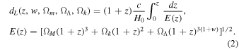
Here Ωm , ΩΛ, and Ωk are the cosmic matter density, dark energy density, and spatial curvature, respectively. We use the following function to estimate cosmological parameters:

where C is the covariance matrix from the combined statistical and systematic uncertainties, and  is the distance modulus measured from the data as described in Section 3.2 and including the bias corrections and host mass step as discussed in Sections 3.5 and 3.6. The model distance modulus
  .
.  is the offset between the assumed SNooPy absolute magnitude of an SN Ia, which is also degenerate with the assumed value of H0, and the best-fit global value.
4. Results
After performing the analysis described in the previous section, we produce the RAISIN NIR-only Hubble diagram shown in Figure 10. The high-z distance measurements are presented in Appendix E. The total rms of the Hubble residuals is 0.167 mag, 18% higher than the Pantheon Hubble residuals. However, the CSP scatter for those SNe with NIR data near maximum light is 0.136 mag, slightly lower than the Pantheon scatter of 0.141 mag, showing the value of well-sampled NIR light curves near maximum light. Future samples with additional epochs near maximum light and a revised NIR model will reduce the scatter well below that achievable from optical data (Avelino et al. 2019). Additional data in the gap between the low-z and RAISIN redshifts would be particularly beneficial in creating an extended NIR Hubble diagram.
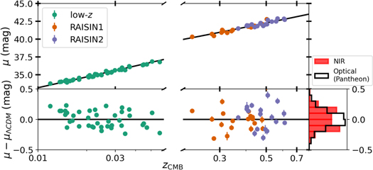
Figure 10. The RAISIN Hubble diagram, with low-z SNe from CSP (green) and high-z samples from RAISIN1 (orange) and RAISIN2 (purple). We show photometric uncertainties only, neglecting the contribution of intrinsic scatter for visual clarity.
Download figure:
Standard image High-resolution image4.1. Ωm and w
By using CosmoMC to constrain cosmological parameters from SNe alone, Figure 11 shows the constraints on nonflat CDM relative to Pantheon and the cosmic acceleration discovery sample from Riess et al. (1998). These data thereby confirm cosmic acceleration with high significance, using a new method and wavelength range that has less sensitivity to dust extinction uncertainties. In a flat universe, from RAISIN SNe alone, we find Ωm = 0.258 ± 0.090.
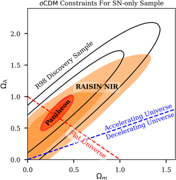
Figure 11. Cosmological parameter measurements from oCDM (a CDM model allowing nonzero curvature) with SNe alone. Open contours show the Riess et al. (1998) discovery sample, red contours show the Pantheon constraints from Scolnic et al. (2018), and the results from RAISIN SNe are in orange. All contours show the 68% and 95% confidence intervals.
Download figure:
Standard image High-resolution imageWith CMB constraints from Planck Collaboration et al. (2020) we find a dark energy equation of state of 1 + w = −0.17 ± 0.12 (Figure 12). This measurement is consistent with the previous NIR measurement from Freedman et al. (2009) of 1 + w = −0.05 ± 0.13 (stat) ± 0.09 (sys) but with smaller uncertainties.
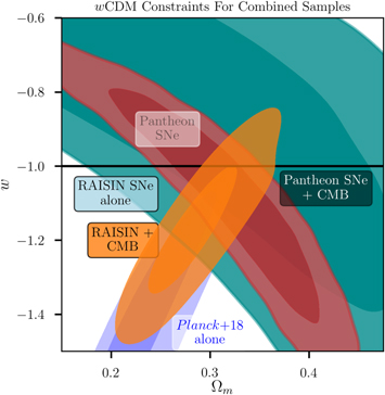
Figure 12. Cosmological parameter measurements from wCDM. RAISIN+CMB cosmological constraints (orange) are consistent with those from the Pantheon sample (black; Scolnic et al. 2018), with a statistically insignificant shift toward phantom dark energy (w < −1). All contours show the 68% and 95% confidence intervals.
Download figure:
Standard image High-resolution imageTable 1. RAISIN Cuts
| CSP DR3 | RAISIN1 | RAISIN2 | ||||
|---|---|---|---|---|---|---|
| Ncut | Nrem | Ncut | Nrem | Ncut | Nrem | |
| ⋯ | 134 | ⋯ | 23 | ⋯ | 22 | |
| σhost < 0.1 mag | 0 | 134 | 2 | 21 | 3 | 19 |
| Spec. SN Ia | 0 | 133 | 1 | 20 | 0 | 19 |
| z > 0.01 | 21 | 116 | 0 | 20 | 0 | 19 |
| Pre-max | 22 | 92 | 0 | 20 | 0 | 19 |
| Pre-max, χ2 cut | 35 | 57 | 0 | 20 | 0 | 19 |
| NIR data | 8 | 49 | 0 | 20 | 0 | 19 |
| SNooPy fitting | 0 | 49 | 0 | 20 | 0 | 19 |
| E(B − V) < 0.3 | 1 | 49 | 0 | 20 | 0 | 19 |
| 0.75 < sBV < 1.18 | 4 | 45 | 1 | 19 | 0 | 19 |
| σ(sBV ) < 0.2 | 2 | 43 | 0 | 19 | 0 | 19 |
| Chauvenet | 1 | 42 | 0 | 19 | 1 | 18 |
Note. The effect of selection cuts on the low-z and RAISIN data sets. These include requiring (1) photometric uncertainty from bright hosts < 0.1 mag, including systematic uncertainty due to subtraction residuals; (2) spectroscopic confirmation that the SN is Type Ia; (3) redshift > 0.01, to limit peculiar velocity errors; (4) data taken before maximum light, before removing points with χ2 > 10 from the light-curve fit; (5) data taken before maximum light, after removing those points (see text); (6) existence of NIR data; (7) successful convergence of the fit to the SNooPy light-curve model; (8) E(B − V) < 0.3; (9) values for the sBV parameter that indicate a normal SN Ia light curve; and (10) two remaining Hubble diagram outliers (SN 2006bt, DES15C1nhv) that fail Chauvenet’s criterion (see text).
Download table as: ASCIITypeset image
Statistical and systematic uncertainties in this analysis are approximately equal. The dominant systematic uncertainty in this measurement is the bias correction—predominantly due to uncertainty in the intrinsic sBV distribution—which will improve with larger sample sizes and improved light-curve fitting methods. The second-largest systematic uncertainty is the size of the NIR mass step (Section 5.1), which will similarly improve with larger sample sizes. The full list of systematic uncertainties on the wCDM model is shown in Table 2 and visually in Figure 13. Though we have attempted to be comprehensive in our accounting of systematic uncertainties, we note that there may be substantial additional uncertainties in this novel measurement that will become more apparent only with larger sample sizes.
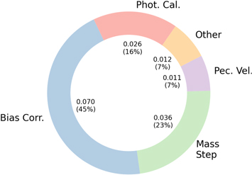
Figure 13. Summary of systematic uncertainties on w for the RAISIN cosmological analysis (Table 2). Bias correction and mass step uncertainties dominate the error budget, with photometric calibration and uncertainties in the peculiar velocities contributing significantly. Other systematic uncertainties are added in quadrature to give the “Other” contribution.
Download figure:
Standard image High-resolution imageTable 2. Summary of Systematic Uncertainties on w from NIR Data Alone
| Error | Δw | Δσw | σw,sys /σstat |
|---|---|---|---|
| All sys. | −0.040 | 0.082 | 0.954 |
| Bias corr. | −0.040 | 0.070 | 0.809 |
| − sBV | −0.040 | 0.069 | 0.805 |
| − AV | 0.000 | 0.009 | 0.099 |
| Mass step | −0.012 | 0.036 | 0.425 |
| Phot. cal. | 0.006 | 0.026 | 0.306 |
| − Low-z | 0.005 | 0.026 | 0.305 |
| − HST | 0.000 | 0.002 | 0.025 |
| Pec. vel. | −0.017 | 0.010 | 0.110 |
| NIR SN model | 0.008 | 0.008 | 0.097 |
| Template flux | 0.008 | 0.008 | 0.097 |
| MW E(B−V) | 0.000 | 0.003 | 0.041 |
| k-corr. | −0.002 | 0.002 | 0.026 |
Note. Summary of systematic uncertainties on the wCDM model with constraints from SNe+Planck. Δw is the shift in w resulting from applying each systematic uncertainty, and Δσw is the additional uncertainty that would need to be added in quadrature to the statistical error to yield the uncertainty on w from a given variant. Note that some variants shift the value of w but do not increase its uncertainties.
Download table as: ASCIITypeset image
4.2. The Hubble Constant
In addition to measuring w, we measure H0 with NIR SN data alone. We use Cepheid distances with CSP and RAISIN SN data to measure the Hubble constant from the distance ladder approach and use SN+CMB data to constrain the H0 parameter with an “inverse distance ladder” approach (e.g., Cuesta et al. 2015) that combines the angular size of the CMB sound horizon with wCDM constraints from CSP, RAISIN, and Planck.
To measure H0 from the distance ladder, we use publicly available Cepheid or tip of the red giant branch (TRGB) distances for all 10 SNe with CSP photometry and with independent TRGB or Cepheid measurements to calibrate the NIR luminosity of SNe Ia. Nine of these SNe—SN 2006D, SN 2007af, SN 2007on, SN 2007 sr, SN 2009Y, SN 2011iv, SN 2012fr, SN 2012ht, and SN 2015F 35 —have redshifts of z < 0.01 and therefore were not included in our baseline sample for measuring w. One SN, SN 2007A, was already included in our sample, as it has a redshift of z = 0.017.
We use a combination of available Cepheid and TRGB distance calibrations (Freedman et al. 2019; Anand et al. 2022; Riess et al. 2021) and take the agnostic approach of giving all available distances as originally provided equal weight. We use Cepheid distances from Riess et al. (2021) for five SNe: SN 2006D, SN 2007A, SN 2009Y, SN 2012ht, and SN 2015F. We use the mean of available Cepheid and TRGB distances for three SNe: SN 2007af (Freedman et al. 2019; Riess et al. 2021), SN 2007sr (Freedman et al. 2019; Anand et al. 2022; Riess et al. 2021), and SN 2012fr (Freedman et al. 2019; Anand et al. 2022; Riess et al. 2021). Finally, we use the mean TRGB distances for two SNe from Freedman et al. (2019) and Anand et al. (2022), SN 2007on and SN 2011iv, which are in the same host galaxy of NGC 1404. These two SNe are fast decliners (Gall et al. 2018 find sBV = 0.57 ± 0.01 and 0.64 ± 0.01 for SN 2007on and SN 2011iv, respectively), with decline rates below our nominal sBV cuts, so we provide results with and without them.
We use these Cepheid and TRGB distances to calibrate the SN luminosity of the CSP and RAISIN samples following the method of Riess et al. (2021). If we include SN 2007on and SN 2011iv in our H0 measurement, we measure H0 = 77.5 ±2.1 km s−1 Mpc−1 from Cepheid+TRGB and H0 = 76.6 ±2.6 km s−1 Mpc−1 from TRGB alone. Excluding the two fast-declining SNe in NGC 1404, however, we measure H0 =75.9 ± 2.2 km s−1 Mpc−1 from Cepheid+TRGB and H0 =72.9 ± 3.0 km s−1 Mpc−1 from TRGB distances alone. We note that the statistical significance of this TRGB measurement with a reduced sample is limited, as we have just three TRGB calibrator galaxies and the measurement is statistically consistent with other recent TRGB-based measurements (Freedman et al. 2019; Anand et al. 2022). The majority of the uncertainty derives from the error in the mean of the modest samples of NIR SN calibrators.
Because our distance measurement method does not correct for any dependence of SN luminosity on sBV and our Hubble flow sample excludes such fast-declining objects (we require sBV > 0.75), it is possible that these fast decliners, which make up a large fraction of the calibrator sample, could bias our results; therefore, our baseline result excludes the fast decliners.
From the inverse distance ladder in a wCDM model, we find a model parameter H0 = 71.2 ± 3.8 km s−1 Mpc−1 (Figure 14). The value of H0 is consistent with the conventional result of 67.4 ± 0.5 assuming ΛCDM with Planck data alone. Independent approaches to measuring SN distances at cosmological redshifts such as this one demonstrate the ways in which future measurements can help determine what role, if any, the present dark energy could play in the tension between local (e.g., Riess et al. 2016; Huang et al. 2020; Pesce et al. 2020; Wong et al. 2020; Foreman-Mackey 2016; Riess et al. 2021) and CMB H0 measurements (e.g., Dhawan et al. 2020).
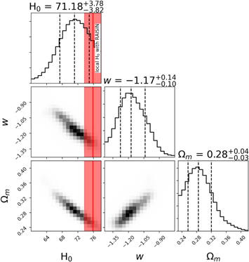
Figure 14. Constraints on H0, w, and Ωm from RAISIN and CMB data combined using an inverse distance ladder method. This figure was generated with the corner package (Foreman-Mackey 2016).
Download figure:
Standard image High-resolution imageThough the uncertainties on these measurements are large, we find that moving to NIR wavelengths does not appear to change the size of the difference between CMB and local H0 measurements (see also Burns et al. 2018; Dhawan et al. 2018).
4.3. Comparing to Optical and Optical+NIR Measurements
Finally, Table 3 compares our NIR-only measurement of w to measurements using optical data alone and optical+NIR data from SNooPy. In computing the optical and optical+NIR measurements, we apply the same base set of systematic uncertainties but add calibration uncertainties at the level of 3 mmag for each PS1 band, 5 mmag for each DES band, and 1% for each optical CSP band (Krisciunas et al. 2017; Burke et al. 2018; Scolnic et al. 2018).
Table 3. Comparing Optical and NIR Measurements of w
| wstat | wstat+sys | σw,sys | Δσw /σstat | |
| Opt. only | −1.099 ± 0.074 | −1.102 ± 0.092 | 0.055 | 0.739 |
| NIR only | −1.128 ± 0.086 | −1.168 ± 0.119 | 0.082 | 0.956 |
| Opt.+NIR | −1.043 ± 0.056 | −1.059 ± 0.074 | 0.048 | 0.864 |
Download table as: ASCIITypeset image
Interestingly, we find substantial shifts when considering optical or optical+NIR data versus NIR data alone. In the NIR-only case versus the optical+NIR case in which NIR data primarily have the effect of constraining the SN color, w shifts by up to 0.11. Though the statistical significance of this shift is not entirely clear given the correlated data and some correlation in the systematic uncertainties, this shift could point to the need for revisions to the NIR or optical SN standardization model in future work, particularly given forthcoming surveys such as the Roman Space Telescope SN survey that will observe in the NIR (Rose et al. 2021a).
Although the sensitivity of the NIR-only measurement to bias correction uncertainties yields a result with significantly higher systematic errors in our baseline analysis, larger sample sizes would result in more precise bias estimations from a better constraint on the redshift-dependent stretch distribution of SNe. However, given that NIR-only approaches will always have difficulty constraining the potential evolution of dust extinction with redshift, we believe that the optimal approach in future work will be an optical+NIR measurement; Table 3 shows that this measurement has the lowest total systematic uncertainty budget of our three wavelength regimes. Though the overall improvement in the precision of w is small, we note that alternative distance measurement methods such as BayeSN (Mandel et al. 2022) appear to more optimally weight the NIR versus optical data and yield significantly reduced distance uncertainties when NIR data are included.
5. Exploring Alternative Analysis Methodologies and Constraining the Mass Step
In this section, we explore variations on our nominal analysis and examine potential systematic uncertainties in the cosmological parameter measurement.
5.1. The Mass Step
Using our nominal distance measurement method, we find a maximum likelihood size of the mass step of ΔM =0.022 ± 0.047 mag at a step location of 10 dex and 0.026 ±0.040 mag at the Ponder et al. (2021) location of 10.44 dex (the step location is fixed during each fit). These results are used to generate the distance measurements in Section 4 above. However, the differences between the NIR and optical measurements are affected by the fact that stretch is correlated with host galaxy mass; our nominal distance method does not fit for stretch, and there is a median difference of ΔsBV =−0.099 between the high- and low-mass subsets of our sample. Correcting for this stretch differential, as done in an optical-only analysis, would have the effect of making the mass step larger.
To measure the mass step in a way that is more comparable to the way optical mass steps are measured, we test the impact of applying an sBV correction to the NIR distances using the best-fit sBV from optical+NIR data. We see a strong trend between Hubble residual and optical+NIR-derived sBV as shown in Figure 15 and find that the scatter in our Hubble residuals is reduced by 10% by making this correction. We do not see a significant change in the dependence of Hubble residual on sBV in the low-z data (slope −0.622 ± 0.189) compared to the high-z data (slope −0.702 ± 0.244).
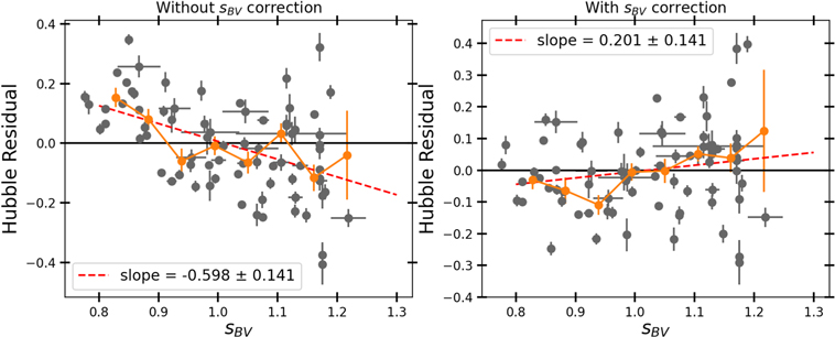
Figure 15. NIR Hubble residuals as a function of sBV , before the Hubble residuals are corrected for sBV (left) and after (right). Correcting for the marginally significant ∼2σ slope in the right panel would shift our high-z distances by just ∼0.015 mag.
Download figure:
Standard image High-resolution imageAfter sBV fitting, we measure a larger mass step, as we would predict, of 0.072 ± 0.041. This result is shown in Figure 16. If, instead, we use the location of the mass step from Ponder et al. (2021) of 10.44 dex, we find a mass step of 0.057 ± 0.035 mag. If we adopt the approximate linear, empirical correction between sBV and Hubble residual shown in Figure 15, instead of using the default SNooPy sBV −luminosity relation, we find consistent steps of 0.086 ± 0.043 mag and 0.094 ± 0.037 mag for 10 and 10.44 dex step locations, respectively. We conclude that there is ∼2σ evidence for a mass step in these data even if we do not a priori assume that the SNooPy luminosity−sBV relation is correct.
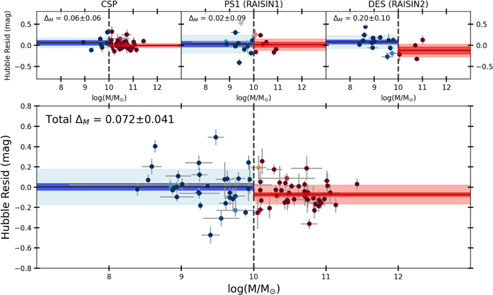
Figure 16. Maximum likelihood, NIR mass step measurements with CSP (top left), RAISIN1 (top middle), RAISIN2 (top right), and all data combined (bottom). Dark shading indicates the uncertainty on the mean for high-mass (red) and low-mass (blue) hosts, while light shading indicates the dispersion of each population. The shading of the points indicates the probability that an SN is in a low-mass host (blue) or high-mass host (red). In this figure (unlike in Figure 10), we correct individual distances for sBV to derive a measurement that is directly comparable to optical analyses. We also simultaneously fit for three z-dependent distance bins to remove the effect of cosmological parameter values on the mass step size.
Download figure:
Standard image High-resolution imageUsing the high-z data alone, we measure a mass step of 0.114 ± 0.081 mag at a step location of 10 dex and a step of 0.122 ± 0.091 mag at 10.44 dex. Unfortunately, the sample is too small to constrain the size of the step with these high-z data alone, which yield a statistically insignificant 1σ evidence for the NIR mass step.
If we use the optical data to measure the mass step with the same SNe, we find a step of 0.11 ± 0.03 mag from SNooPy and 0.08 ± 0.03 mag from SALT3 (the same step size is measured from SALT2). These are consistent with optical mass steps in the literature, which can range from 0.04 ± 0.019 mag from DES (Smith et al. 2020) to 0.119 ± 0.032 from the Nearby Supernova Factory (Aldering et al. 2002; Rigault et al. 2020); the largest data set (Pantheon; Scolnic et al. 2018) yields a step of 0.072 ± 0.01. 36
These mass step results qualitatively support—albeit with limited significance—the findings of Ponder et al. (2021) and Uddin et al. (2020), who also found evidence that the NIR mass step was of order the same size as the optical mass step.
5.2. Comparing to Alternative Distance Measurement Methods
5.2.1. NIR Distances from BayeSN
Although we have not yet simulated distance biases with the BayeSN SED model, we did compare our SNooPy distances before bias correction to raw BayeSN distances that assume a fixed stretch and zero host dust extinction AV , analogous to the approach we adopted for SNooPy. We fix the BayeSN primary intrinsic component θ = −1, approximately equivalent to our chosen SNooPy sBV = 1. We use the same time of B-band maximum light for both SNooPy and BayeSN and fit only the NIR light-curve data to obtain photometric distance estimates.
As demonstrated in Figure 17, these distances are consistent across the redshift range of our sample, with the average difference between BayeSN and SNooPy distances changing by just 2 mmag from the low-z to high-z samples. As SNooPy has rarely been used at high redshift, this consistency between the two models gives us confidence that the raw distances that we measure with SNooPy are robust.
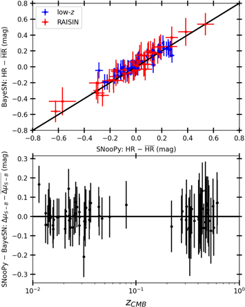
Figure 17. Top: SNooPy vs. BayeSN Hubble residuals for the low-z (blue) and RAISIN (red) samples. Bottom: SNoopy distance moduli minus BayeSN distance moduli as a function of redshift with an average redshift-independent offset removed (cosmological parameter measurements are not affected by a global offset). The average value of the SNooPy distance modulus minus the BayeSN distance modulus changes by only 2 mmag between the low-z and RAISIN samples.
Download figure:
Standard image High-resolution image5.2.2. Optical Distances from SALT3 and SNooPy
In Table 4, we explore the differences between several methods of measuring NIR, optical, and optical+NIR distances. We compare the baseline NIR-only distances to optical+NIR distances with both the baseline RV = 1.5 and an MW-like RV = 3.1. We also compare to optical distances from SALT3, and finally, we use an approach where optical+NIR data are first used to determine sBV and then sBV is fixed to that value in an NIR-only fit that measures the distance. This essentially allows the NIR distances to include the anticipated sBV −luminosity relation.
Table 4. Optical+NIR Distance Comparisons
| Δμ (mag) | |
|---|---|
| Optical+NIR (RV = 1.5) | 0.011 ± 0.030 |
| Optical+NIR (RV = 3.1) | −0.065 ± 0.032 |
| Optical with SALT3 | 0.005 ± 0.038 |
| Optical+NIR sBV , NIR dist. | −0.016 ± 0.027 |
Note. For optical+NIR analysis methods without bias corrections, the difference between low- and high-z distances relative to the baseline NIR-only method.
Download table as: ASCIITypeset image
We find Hubble residual differences of ∼1%−2% between our baseline NIR method and methods using optical data and the default SNooPy value of RV = 1.5 (Folatelli et al. 2010). With RV = 3.1, the difference in distances is much larger, at 0.065 mag between low and high redshift, though we note that using this value of RV increases the Hubble residual scatter by 28%. In an NIR-only analysis, however, using RV = 3.1 changes the distances by just ∼0.02−0.04 mag owing to the lower sensitivity of the NIR to the value of RV . Because we allow negative extinction in this analysis and because SNooPy does not model the intrinsic correlation between color and luminosity, the RV parameter is more analogous to the nuisance parameter β in the Tripp relation than to a physical dust law.
The difference between our baseline distances and SALT3 distances is just 0.005 ± 0.038 mag. Although this difference in distance is small, the bias corrections shown in Figure 7 are ∼0.05 mag smaller in the NIR-only distances, increasing the potential discrepancy between SALT3 and the baseline NIR measurement. However, given the large uncertainties on the distance in measurement, a SALT3-based (or SALT2-based) analysis would still yield a consistent measurement of w.
Finally, the procedure of adjusting the NIR distances by a value of sBV measured in the optical results in a statistically insignificant −0.016 ± 0.027 mag change. The lack of a small sBV correction in our baseline analysis therefore does not appear to have a significant impact on the resulting cosmological parameter estimation. We also explore altering the semiarbitrary sBV cuts in our baseline distance measurements, particularly given that the sBV values tend to cluster near ∼1.18, perhaps due to a limited high-sBV training sample in SNooPy. Fortunately, we find that our analysis is relatively insensitive to the minimum and maximum sBV ; both a “loose” cut of 0.6 < sBV < 1.3 and a “tight” cut of 0.8 < sBV < 1.15 change the average Hubble residual by just 7 mmag when comparing SNe at z < 0.1 to those at z > 0.1. The mass step measurement is changed by less than 0.01 mag.
In Figure 18, we examine the dispersion of Hubble residuals for different methods that use optical data. We find that the Hubble residual dispersion is lowest when using the optical+NIR with RV = 1.5 (0.140 mag) or the SALT3 model (0.130 mag). SALT3 appears to standardize SNe Ia more precisely than SNooPy at high redshift, while SNooPy distances are more precise than SALT3 distances for the CSP data on which SNooPy was trained. The SALT3 results are nearly the same as those from SALT2, which was used for most previous optical-only analyses.
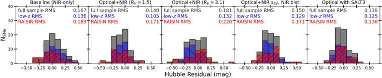
Figure 18. Hubble residual scatter for different analysis variants. From left to right, we show our baseline NIR-only Hubble residuals, optical+NIR SNooPy distances with RV = 1.52 (Folatelli et al. 2010), optical+NIR SNooPy Hubble residuals with RV = 3.1, NIR SNooPy Hubble residuals after applying the sBV parameters measured from optical+NIR data, and optical SALT3 Hubble residuals. The SALT3 panel removes two CSP SNe with colors that are too red (c > 0.3) to pass standard SALT cosmology cuts; with these SNe included, scatter increases negligibly to 0.132 mag in the CSP sample.
Download figure:
Standard image High-resolution imageIf an optical versus NIR difference becomes statistically significant in future work, it could point to unrecognized systematic uncertainties in analyses with optical data, NIR data, or both. In optical analyses, the G10 scatter model is a source of significant uncertainty in correcting for distance-dependent biases (Scolnic et al. 2018; Brout et al. 2019b), and proposed alternative scatter models could shift w by 4% (Brout & Scolnic 2021). In the NIR, differences in stretch−luminosity correlations between Burns et al. (2014) and Burns et al. (2018), for example, may point to systematic uncertainties in SNooPy NIR standardizations. These results show that NIR observations constitute an extremely useful consistency check on optical analyses.
5.3. The Late-time NIR Model
Our Hubble diagram compares SNe observed near maximum light in the low-z CSP sample to SNe observed only at later phases in the higher-z RAISIN sample; the initial NIR epoch in RAISIN occurred at +9 rest-frame days on average. This could introduce systematic uncertainty if the SN standardization model is not as accurate at late times as it is near maximum light, where most previous NIR data exist. Although we account for this systematic uncertainty by using two SN Ia standardization models, both use much of the same training data.
To investigate potential biases due to the phase at which each SN was observed in the NIR, we investigated whether there is a trend in Hubble residuals as a function of the median phase at which each SN was observed. By comparing the Hubble residuals of SNe observed at a median phase of <+ 15 days to those observed at a median phase of >+ 15 days (+15 days is approximately the sample median), we detected a “step” in the NIR Hubble residuals at 3σ significance. This step appears to show that RAISIN SNe Ia observed at a phase of >+ 15 days are fainter by 0.164 ± 0.051 mag than RAISIN SNe Ia observed at a median phase of <+ 15 days. Though this trend is potentially concerning, we note that the difference in stretch between the early- and late-observed samples is 0.12, which could explain ∼0.05 mag of the ∼0.16 mag difference (Figure 15). This selection bias could be caused by the fact that low-stretch SNe are intrinsically fainter, so it may have been harder to classify them and subsequently trigger HST observations prior to maximum light.
To inspect potential biases in the SNooPy model as a function of phase, in Figure 19 we show the SNooPy Y-band template alongside the CSP and RAISIN observations after the observed data have been converted to the rest frame. Both the high- and low-z data agree relatively well with the SNooPy model, albeit with slight offsets at +10 days < phase <+20 days of ∼0.05 mag. These offsets suggest that the late-phase NIR SNooPy model should be adjusted as more data become available but would only shift the mean high-z distance measured here by approximately 0.02 mag. The variance of the NIR data also appears to increase slightly near the phase at which most of the later RAISIN observations occur, while observations near maximum light have the lowest scatter. The slightly higher scatter of the RAISIN magnitudes compared to CSP might also be an indication of K-correction uncertainties in the high-z distances. We observe similar trends when comparing the J-band SNooPy model to our data.
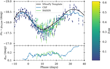
Figure 19. The SNooPy model (black) compared to CSP (blue) and RAISIN (red) measurements after using the SNooPy K-corrections and the cosmological distance to convert the observations to rest-frame absolute magnitude. Solid lines in the top panel show the rolling means of the CSP and RAISIN absolute magnitudes, and the rolling standard deviation, with the average peculiar velocity error and photometric noise subtracted in quadrature, is shown in the bottom panel. NIR SN Ia observations appear to have the lowest rms near maximum light and slightly higher rms from ∼10 to 25 days.
Download figure:
Standard image High-resolution imageThe apparent dependence of Hubble residual on the phase at which an SN was observed could also be due to subtle errors in the relationship between SN luminosity and sBV or the fact that the NIR SN color−luminosity dependence differs significantly from the relation that would be expected from dust extinction alone. Although retraining the SNooPy model is beyond the scope of this work and will likely require significant additional rest-frame NIR data to be robustly redetermined, additional low-z data and model retraining are important ways in which future NIR analyses could be improved.
6. Discussion
Although this study reaffirms the existence of cosmic acceleration and establishes the value of NIR SN Ia data for cosmological measurements, much of the value of this data set will be in preparing for NIR SN Ia samples from the Roman Space Telescope. Although the SN survey strategy is not yet finalized, Roman will observe in the rest-frame NIR to z ≈ 0.7, the regime in which cosmological parameter constraints from SNe Ia will likely be more precise than volume-limited baryon acoustic oscillations (Weinberg et al. 2013). Measuring the most precise cosmological constraints from these data will be the path to obtaining the best possible constraints on cosmological parameters.
With Roman on the horizon, the systematic error budget presented here suggests a path forward for improved NIR cosmological constraints. Here is what we need:
- 1.Larger photometric NIR samples with coverage near maximum light across multiple photometric systems to improve calibration systematics.
- 2.Larger photometric and spectroscopic NIR samples to improve training of models, and optical-to-NIR measurements of the SN Ia dispersion to constrain any redshift dependence of the value of RV .
- 3.Optical-to-NIR SN Ia SED models and standardization methods that separate SN Ia intrinsic dispersion from the effects of host galaxy dust as a function of wavelength and improve the modeling of high-stretch (slowly declining) SNe.
- 4.Improved constraints on the host galaxy mass step and other host galaxy dependences as a function of wavelength to break degeneracies with dust properties.
- 5.An untargeted NIR low-z sample with well-understood selection effects.
These improvements would improve the accuracy of the cosmological measurement presented here even without obtaining additional high-z data. A public release of CSP-II NIR spectra and photometry will address several of these key points (Hsiao et al. 2019; Phillips et al. 2019). As we enter the Roman era, new data will also reduce bias correction systematics by constraining the distribution of SN shape and color as a function of redshift. We elaborate on a number of these potential improvements below.
6.1. NIR Dispersion Model
The NIR dispersion model measured both in this work and in the BayeSN SED model shows that NIR distances offer significant independent leverage to constrain distance measurements compared to those obtained only with optical data. Further, NIR data, in combination with optical, provide additional leverage to improve constraints on both RV and AV , as demonstrated in recent analyses that use NIR data to break the degeneracy between host galaxy dust and intrinsic SN physics (Thorp et al. 2021; Mandel et al. 2022).
In this study, we see that, even without shape and color corrections, just three epochs of NIR data at ∼10−20 days after maximum light are sufficient to constrain dark energy properties. It is possible that even fewer epochs or filters would still yield competitive cosmological constraints, though additional epochs and filters give the valuable ability to avoid data outliers and to constrain dust properties. Much of the systematic uncertainty in this analysis stems from the fact that these SNe were selected for spectroscopic follow-up in the optical. In large, untargeted NIR samples like those from Roman, this source of systematic uncertainty will vanish.
6.2. Building a New, Well-calibrated NIR SED Model
SN Ia analyses and standardization models in the NIR are currently limited by the sample sizes of well-calibrated data sets, both photometric and spectroscopic, which introduce substantial calibration systematics and uncertainties in the precision of the standardization model training itself. New, well-calibrated NIR samples from CSP-II, SIRAH, VISTA, UKIRT (Konchady et al. 2022), and eventually Roman will be needed for improved model training. Simultaneous NIR spectroscopy will also be important for a better understanding of K-corrections. The SIRAH sample in particular, with extremely well-calibrated photometry and grism spectroscopy tied to ground-based NIR observations, will be a powerful link between precise NIR cosmological analyses from space and the ground.
This analysis shows that the NIR+optical measurement of w has similar precision to the optical measurement alone. Although we find that systematic uncertainties on w are lowest when we use NIR data in combination with optical, there is no improvement in the precision of cosmological parameter measurements when adding NIR data in this analysis. This is likely because our light-curve fitting approaches are not yet optimally weighting the SN data at different wavelengths, a problem that previous studies have found can be addressed with improved uncertainty treatments in SN standardization models (Mandel et al. 2011, 2022).
6.3. The Mass Step
The underlying cause of the host galaxy mass step is a subject of debate, with numerous explorations of alternative global host galaxy dependencies (Hayden et al. 2013; Pan et al. 2014) or relationships between Hubble residuals and local host galaxy properties near the SN location (Rigault et al. 2013; Jones et al. 2015a; Rigault et al. 2015; Jones et al. 2018b; Kim et al. 2018; Rigault et al. 2020; Roman et al. 2018; Kelsey et al. 2021). The degeneracy between physical effects, potential data reduction artifacts (Solak et al. 2021), and dust has made measuring the wavelength dependence of the host galaxy mass step, as well as other host galaxy dependencies, extremely important for next-generation cosmological measurements. Measurement of whether a step-like dependence of NIR Hubble residuals on global or local galaxy color (e.g., Roman et al. 2018; Jones et al. 2018b; Kelsey et al. 2021) would be particularly interesting to understand the effects of dust or progenitor ages on SN distance measurements. Previous measurements of the mass step in the NIR have been limited by sparse data (Ponder et al. 2021) and the need to include optical data with the NIR observations to constrain the best-fit parameters such as sBV and AV (Uddin et al. 2020). Flexible simulation-based approaches (e.g., Pierel et al. 2021) will be necessary to fully understand the impact of different SN–host relationships on cosmological parameter measurements.
Although the galaxy-targeted nature of the CSP sample has made measuring the mass step in this work difficult (nearly all CSP galaxies are in the “high-mass” regime), we do find evidence suggesting that the mass step in the NIR is about the size of the mass step in the optical. We note that our results are not in tension with other recent NIR mass step results, including those of Johansson et al. (2021), who saw that the mass step was insignificant in the JH bands and less significant (∼2σ) in the Y band. Our distances primarily probe the rest-frame Y band, albeit with some i- and J-band overlap, where Johansson et al. (2021) find a mass step of approximately 0.07 ± 0.03 mag. However, our results do not favor the conclusion of Brout & Scolnic (2021) that the mass step is caused by variations in dust properties, as the effect of variation in RV should decrease by a factor of ∼3 between, e.g., rest-frame V and rest-frame Y. Further study of the origin of the mass step is clearly needed, and larger infrared samples may prove useful.
Future measurements of this and other host galaxy dependencies as a function of wavelength may be necessary to separate intrinsic color, dust, other SN Ia physics, or even multiple SN Ia progenitor models. For example, when measuring the mass step, we did not fit for individual RV values, as was done in Johansson et al. (2021), or simultaneously constrain the population distribution of RV values, as was done in Thorp et al. (2021); these methods can help to disentangle the role of dust in the mass step’s size. Although SNe Ia are used as an empirical tool for measuring distance, understanding the objects and their connection to stellar populations is also valuable in itself. The evolution of stellar populations and of SN Ia progenitors across the long span of cosmic time that Roman will provide gives an opportunity to understand the nature of SN progenitors and their environments and to use them for more precise cosmological measurements.
7. Conclusions
We present photometric measurements, a Hubble diagram, and NIR-only cosmological constraints from the RAISIN survey. SN candidates were observed in cycles 20 and 23 by HST and combined with low-z, NIR-observed SNe from CSP to yield an NIR Hubble diagram and a better understanding of cosmological parameter measurements in the NIR. From CSP data we build a new, optical-to-NIR dispersion model for SNe Ia to predict distance-dependent biases and measure the independence of SN Ia distances in the optical and NIR. We find that NIR-derived distances are well correlated with distances derived from optical data but offer some independent information. The dispersion of our NIR-only distances is 0.18 mag, ∼25% larger than the Pantheon sample at 0.141 mag but not standardized using shape or color information. When measuring the host galaxy mass step after applying shape corrections to our distances, in order to match the procedures used in optical analyses, we measure an NIR mass step of 0.072 ± 0.041 mag at a step location of 10 dex and 0.123 ± 0.034 mag at a step location of 10.44 dex.
In combination with CMB constraints from Planck Collaboration et al. (2020) and assuming a flat wCDM model, we measure 1 + w = –0.17 ± 0.12 (stat+sys), consistent with the ΛCDM expectation of w = −1. This NIR measurement of w may embed unknown systematic uncertainties that will become apparent when future, larger NIR samples are analyzed. The dominant systematic uncertainties in this analysis stem from bias corrections, which will be improved by future SN standardization models that extend to the NIR; building these models will be facilitated by larger NIR sample sizes on the way from CSP-II, SIRAH, VISTA, and UKIRT. We find that combined cosmological parameter measurements from optical+NIR data appear to have lower systematic uncertainties than when using optical data alone. We also see shifts in w of up to 0.1 among optical, optical+NIR, and NIR data alone, pointing to the possibility of inconsistency in the optical versus NIR SN standardization models.
We also measure H0 = 75.9 ± 2.2 km s−1 Mpc−1 from a local distance ladder approach tied to eight NIR-observed SNe Ia with Cepheid or TRGB distances versus H0 = 71.2 ±3.8 km s−1 Mpc−1 using a so-called “inverse distance ladder” approach anchored to CMB measurements of the angular size of the sound horizon. Future NIR measurements can help to constrain whether the present dark energy density or systematic uncertainties due to SN Ia dust could play any role in the H0 tension.
Finally, these data will help us to better understand the behavior and standardization of SNe Ia in the NIR and assist the community in preparing for data from the Roman Space Telescope. Improved dispersion models will help improve distances by using an optical+NIR combination, and wavelength-dependent measurements of the dependence of SN Ia distance measurements on host galaxy properties will break the degeneracies with dust properties. When combined with future data sets from SIRAH and improved SN Ia standardization models that can be trained with this data set, we hope the data published here will have legacy value for the SN Ia community in the Roman Space Telescope era. 37
We would like to acknowledge that much of the data and analysis in this manuscript were made possible through the work of our friend and colleague Dr. Andrew S. Friedman, who passed away during the final stages of this project. We would also like to thank G. Narayan and N. Drakos for useful discussions and their assistance with HST photometry and K-corrections. We would like to thank R. Kessler for implementing the latest SNooPy model in SNANA and C. Rojas-Bravo for assistance with the spectra. We would also like to thank the anonymous referee for many helpful suggestions.
Support for this work was provided by a Gordon and Betty Moore Foundation postdoctoral fellowship to D.O.J. at the University of California, Santa Cruz, and by NASA through the NASA Hubble Fellowship grant HF2-51462.001 awarded by the Space Telescope Science Institute, which is operated by the Association of Universities for Research in Astronomy, Inc., for NASA, under contract NAS5-26555. The Cambridge University team acknowledges support from the European Research Council under the European Union’s Horizon 2020 research and innovation program (ERC grant agreement No. 101002652); the ASTROSTAT-II collaboration, enabled by the Horizon 2020, EU grant agreement No. 873089; and the Cambridge Centre for Doctoral Training in Data-Intensive Science funded by the UK Science and Technology Facilities Council (STFC). L.G. acknowledges financial support from the Spanish Ministerio de Ciencia e Innovación (MCIN), the Agencia Estatal de Investigación (AEI) 10.13039/501100011033, and the European Social Fund (ESF) “Investing in your future” under the 2019 Ramón y Cajal program RYC2019-027683-I and the PID2020-115253GA-I00 HOSTFLOWS project, from Centro Superior de Investigaciones Científicas (CSIC) under the PIE project 20215AT016, and the program Unidad de Excelencia Mara de Maeztu CEX2020-001058-M. M.R.S. is supported by the NSF Graduate Research Fellowship Program under grant 1842400. The UCSC team is supported in part by NASA grants 14-WPS14-0048, NNG16PJ34C, and NNG17PX03C; NSF grants AST-1518052 and AST-1815935; NASA through grant No. AR-14296 from the Space Telescope Science Institute, which is operated by AURA, Inc., under NASA contract NAS 5-26555; the Gordon and Betty Moore Foundation; the Heising-Simons Foundation; and fellowships from the Alfred P. Sloan Foundation and the David and Lucile Packard Foundation to R.J.F. Based on observations with the NASA/ESA Hubble Space Telescope obtained from the Data Archive at the Space Telescope Science Institute, which is operated by the Association of Universities for Research in Astronomy, Inc., under NASA contract NAS5-26555. Support for program Nos. 13046 and 14216 was provided through grants from the STScI under NASA contract NAS5-26555. The Carnegie Supernova Project has been supported by the National Science Foundation under grants AST0306969, AST0607438, AST1008343, AST1613426, AST1613455, and AST1613472. L.K. thanks the UKRI Future Leaders Fellowship for support through the grant MR/T01881X/1. This research has made use of the NASA/IPAC Extragalactic Database (NED), which is funded by the National Aeronautics and Space Administration and operated by the California Institute of Technology.
This paper includes data gathered with the 6.5 m Magellan Telescopes located at Las Campanas Observatory, Chile. Some of the observations reported here were also obtained at the MMT Observatory, a joint facility of the University of Arizona and the Smithsonian Institution, and the W. M. Keck Observatory, which is operated as a scientific partnership among the California Institute of Technology, the University of California, and the National Aeronautics and Space Administration. The Observatory was made possible by the generous financial support of the W. M. Keck Foundation. The authors also wish to recognize and acknowledge the very significant cultural role and reverence that the summit of Maunakea has always had within the indigenous Hawaiian community. We are most fortunate to have the opportunity to conduct observations from this mountain. This paper also uses observations obtained at the international Gemini Observatory, a program of NSF’s NOIRLab, which is managed by the Association of Universities for Research in Astronomy (AURA) under a cooperative agreement with the National Science Foundation on behalf of the Gemini Observatory partnership: the National Science Foundation (United States), National Research Council (Canada), Agencia Nacional de Investigacin y Desarrollo (Chile), Ministerio de Ciencia, Tecnologa e Innovacin (Argentina), Ministrio da Cincia, Tecnologia, Inovaes e Comunicaes (Brazil), and Korea Astronomy and Space Science Institute (Republic of Korea). Finally, we include data acquired at the Anglo-Australian Telescope. We acknowledge the traditional owners of the land on which the AAT stands, the Gamilaroi people, and pay our respects to elders past and present.
Software: PythonPhot (Jones et al. 2015b), hstphot (https://github.com/srodney/hstphot), TinyTim (Krist et al. 2011), HOTPANTS (Becker 2015), ZOGY (Zackay et al. 2016), corner (Foreman-Mackey 2016), SNANA (Kessler et al. 2010), LePHARE (Arnouts & Ilbert 2011), SNooPy (Burns et al. 2011, 2014), RVSAO (Kurtz & Mink 1998), Marz (Hinton et al. 2016).
Appendix A: Photometric Measurements from HST
In this appendix, we describe the photometric measurement of RAISIN SNe from HST. The photometric measurements themselves are given in Appendix B.
First, we used AstroDrizzle to combine RAISIN FLT images downloaded from the Mikulski Archive for Space Telescopes (MAST) and created geometric distortion-corrected images for each epoch of each SN. For a given SN, each epoch of observations is drizzled; then the output, drizzled images are aligned to a reference image via tweakreg so that SN coordinates are consistent in all epochs; and then the data from each epoch are redrizzled. Finally, we subtract the drizzled template image from each image containing the SN. We make use of sndrizpipe,
38
a pipeline for HST drizzling and image subtraction originally written for the CANDELS and CLASH HST Multi-Cycle Treasury programs (Grogin et al. 2011; Postman et al. 2012) that has continued being actively developed in the past few years. Images were drizzled to 011 pixel−1, slightly smaller than the native pixel scale of WFC3, to improve the resolution of the HST PSF (we found minimal differences between 0
09 and 0
13 pixel−1 choices). The photometric zero-points that we use are derived from the latest HST calibrations of Bohlin et al. (2020).
SN positions from discovery data or optical imaging are known to approximately 1″ precision or better and are given in Table 5. We use centroiding algorithms from the hstphot 39 and PythonPhot (Jones et al. 2015b) packages to refine those positions. The best centroid was given by the weighted average of coordinates measured from F125W images for RAISIN1 and F160W images for RAISIN2. Because SNe Ia are fainter in redder bands and host galaxies are often brighter, coordinates from F125W images tend to be more reliable when available.
Table 5. RAISIN Coordinates, Redshifts, and Discovery Dates
| ID | α | δ | zHelio | zCMB | zsource a | MJDdisc |
|---|---|---|---|---|---|---|
| PS1-480464 | 09:59:12.147 | 03:13:17.555 | 0.220 | 0.221 | host | 55243 |
| PS1-450082 | 23:33:25.446 | 00:18:37.609 | 0.250 | 0.249 | SN | 56233 |
| PS1-540087 | 22:21:30.369 | 00:07:46.110 | 0.275 | 0.275 | host | 56505 |
| PS1-520188 | 14:22:05.831 | 52:32:40.679 | 0.280 | 0.280 | host | 56469 |
| DES16E2cxw | 00:40:42.701 | −43:55:18.948 | 0.293 | 0.293 | host | 57686 |
| PS1-440005 | 03:31:57.424 | −28:53:00.481 | 0.306 | 0.306 | host | 56206 |
| PS1-520062 | 16:17:48.345 | 54:37:59.502 | 0.308 | 0.308 | SN | 56442 |
| PS1-500100 | 08:46:33.237 | 45:21:21.978 | 0.310 | 0.311 | host | 56383 |
| PS1-500301 | 14:22:11.455 | 52:37:54.908 | 0.325 | 0.325 | host | 56394 |
| PS1-470041 | 08:45:21.034 | 44:45:17.194 | 0.331 | 0.332 | host | 56290 |
| PS1-480794 | 09:58:10.055 | 01:21:50.792 | 0.334 | 0.334 | host | 56332 |
| PS1-490521 | 09:55:27.619 | 01:34:30.925 | 0.340 | 0.341 | SN | 56358 |
| PS1-470110 | 03:28:16.989 | −28:37:23.988 | 0.346 | 0.346 | host | 56299 |
| DES16E2clk | 00:36:48.876 | −44:08:23.460 | 0.367 | 0.367 | SN | 57680 |
| DES16C2cva | 03:34:44.035 | −29:19:02.028 | 0.403 | 0.403 | host | 57686 |
| DES15X2kvt | 02:21:46.262 | −05:38:23.640 | 0.404 | 0.404 | SN | 57298 |
| PS1-450339 | 02:25:09.004 | −03:21:12.182 | 0.410 | 0.410 | host | 56234 |
| DES15E2nlz | 00:35:51.350 | −44:40:36.444 | 0.410 | 0.410 | SN | 57356 |
| PS1-530251 | 22:18:32.238 | 01:06:53.316 | 0.413 | 0.412 | host | 56477 |
| DES15C1nhv | 03:39:00.948 | −27:50:35.520 | 0.421 | 0.421 | host | 57355 |
| PS1-550202 | 23:27:11.964 | −00:46:59.074 | 0.422 | 0.421 | host | 56558 |
| PS1-490037 | 09:59:49.727 | 00:48:59.738 | 0.422 | 0.423 | host | 56354 |
| DES16E2cqq | 00:39:50.076 | −43:33:53.388 | 0.426 | 0.426 | host | 57682 |
| PS1-440236 | 02:28:24.442 | −04:25:28.243 | 0.430 | 0.429 | host | 56197 |
| PS1-470240 | 08:42:53.508 | 45:54:04.910 | 0.430 | 0.431 | SN | 56302 |
| DES16X1cpf | 02:16:49.512 | −04:13:06.096 | 0.436 | 0.436 | host | 57681 |
| DES15E2mhy | 00:41:17.134 | −43:53:10.104 | 0.439 | 0.439 | host | 57329 |
| PS1-560027 | 02:23:24.170 | −03:05:02.026 | 0.440 | 0.439 | SN | 56167 |
| DES16E1dcx | 00:35:52.440 | −43:21:29.232 | 0.453 | 0.453 | host | 57694 |
| DES15X2nkz | 02:22:13.210 | −05:52:18.228 | 0.469 | 0.469 | host | 57356 |
| DES16S1bno | 02:50:03.823 | −00:01:17.724 | 0.470 | 0.470 | SN | 57653 |
| PS1-540118 | 23:27:17.446 | −00:02:53.063 | 0.477 | 0.477 | host | 56508 |
| PS1-560054 | 23:33:10.992 | −00:20:11.692 | 0.482 | 0.480 | host | 56562 |
| DES16S2afz | 02:46:24.329 | −01:13:31.044 | 0.483 | 0.483 | host | 57626 |
| DES16E2rd | 00:32:21.334 | −43:50:46.032 | 0.494 | 0.494 | host | 57629 |
| DES16X3zd | 02:26:56.465 | −04:25:09.804 | 0.495 | 0.495 | host | 57325 |
| PS1-510457 | 12:25:33.373 | 48:08:11.868 | 0.502 | 0.503 | host | 56420 |
| DES16S1agd | 02:52:20.062 | −00:54:40.284 | 0.504 | 0.504 | host | 57633 |
| DES15C3odz | 03:27:55.027 | −28:33:52.092 | 0.508 | 0.508 | host | 57378 |
| PS1-520107 | 12:16:38.631 | 47:48:57.881 | 0.519 | 0.520 | SN | 56444 |
| DES16C1cim | 03:39:30.362 | −26:38:57.048 | 0.531 | 0.531 | host | 57667 |
| DES16C3cmy | 03:27:13.440 | −27:29:20.724 | 0.556 | 0.556 | host | 57680 |
| DES15E2uc | 00:37:53.419 | −43:18:51.552 | 0.566 | 0.566 | host | 57252 |
| DES15X2mey | 02:20:30.785 | −06:26:47.472 | 0.608 | 0.608 | host | 57327 |
| DES16X3cry | 02:24:10.548 | −03:49:51.996 | 0.612 | 0.612 | host | 57686 |
Notes. Coordinates, redshifts, and approximate discovery MJD (the first S/N > 5 detection) for RAISIN SNe.
a SN redshifts are accurate to σz ≃ 0.01, while host redshifts are accurate to better than σz = 0.001.Download table as: ASCIITypeset image
Using the measured SN coordinates, we performed aperture photometry with a fixed 04 radius using the zero-points and aperture corrections determined from standard star observations.
40
We found that, due to the undersampled and somewhat variable HST PSF, aperture photometry was more reliable than PSF photometry for these images. There are few stars in a typical RAISIN frame from which to determine the PSF on an epoch-by-epoch basis, and, likely due to the breathing of HST and the undersampled WFC3 PSF, we found that the PSF was too variable for a PSF model based on archival data to be sufficient. By performing artificial star tests, we found that we were unable to perform PSF photometry without introducing millimagnitude-level biases.
As the drizzling process produces pixels with correlated noise, uncertainties were estimated by planting 1000 fake stars per epoch at random locations. Fake stars were generated using a P330E PSF model (again created using hstphot), and each fake star had a magnitude equal to the measured SN mag in a given epoch. The dispersion in these fake star magnitudes was added in quadrature to the Poisson noise from the SN to give the total uncertainty due to sky background variation, correlated pixels, and Poisson noise. Given that our final pixel scale is near the native pixel size of WFC3-IR, the noise in the recovered stars is likely dominated by Poisson noise of the sky background.
The expected bias in the photometry given the centroid uncertainties derived above is derived by Rest et al. (2014), their Appendix D. This requires an estimate of how much the magnitude changes when the coordinate is incorrect by 1 pixel. P330E images show that this is approximately 0.022 mag for a 011 pixel scale, but typical centroid uncertainties are closer to ∼0.02 pixels. We corrected for these biases, but in practice we find that they are typically <1 mmag.
A.1. Host Galaxy Noise
SNe Ia on top of bright host galaxies can have biased measurements or underestimated errors. The additional noise introduced by a bright host galaxy tends to create significant subtraction residuals by increasing the effect of small PSF changes between the template and SN images. We occasionally see significant dipole-like subtraction artifacts.
To model this effect, we used TinyTim to create up to 25 fake stars near the same host galaxy as each SN. We require that the fake stars are at least 07 from the SN position and from each other, which is >4 times the FWHM of the F160W PSF. We cannot measure the noise at the exact location of the SN, but we can gain a statistical sense of the noise as a function of host galaxy surface brightness from these fake stars.
The results of this test are shown in Figure 20. Small error bars give the uncertainty on the average magnitude in each surface brightness bin, and large error bars give the dispersion of the fake magnitudes in each bin. To compute more realistic uncertainties, we then subtract the measured magnitude uncertainties in quadrature from the total magnitude dispersion of the fake stars. These quantities give the extra uncertainty that should be added in quadrature to each SN magnitude as a function of the brightness of the host galaxy underneath the SN. SNe with estimated host galaxy uncertainties of greater than 0.1 mag are removed from the sample; we chose this cut based on visual inspection, which shows that such SNe typically have subtraction artifacts likely due to misalignments or “breathing” of HST and are unlikely to provide reliable, unbiased photometry. Our team attempted applying convolutional subtraction algorithms to the data including HOTPANTS (Becker 2015) and ZOGY (Zackay et al. 2016) but did not achieve improved results for these bright hosts. Five SNe were removed from the final analysis based on excessive host galaxy noise.
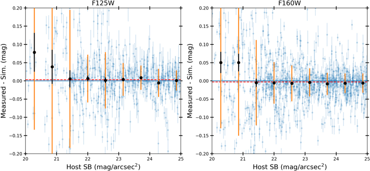
Figure 20. Dispersion of fake star magnitudes as a function of host galaxy surface brightness at the SN location for F125W (left) and F160W (right). Large error bars (orange) show the dispersion, while small error bars (green) show the error on the mean. We restrict to the sample of SNe with predicted host galaxy error less than 0.1 mag and verify with visual inspections that the subtracted images for these SNe appear reliable.
Download figure:
Standard image High-resolution imageA.2. Residual SN Flux in Template Imaging
The RAISIN programs took HST template imaging between 129 and 285 days after the estimated time of maximum light for subtracting from the HST images with SN light. To test that our time interval between SN images and template images was sufficient, we used early- and late-time observations of SN 2012fr, which has YJ imaging at ∼150 days after maximum light from Contreras et al. (2018). With these data, we can extrapolate to later times to estimate the residual flux of RAISIN SNe at the time the template was taken.
For all RAISIN SNe, we use this estimated template flux to correct the magnitudes of RAISIN SN observations for which the closest rest-frame band is Y. Due to the faster decline of SNe in the J band, the J-band correction is expected to be negligible. To account for variability in the typical decline rate of SNe at late times in the NIR, we created a version of our analysis in which we conservatively increase the predicted late-time template flux by 0.5 mag for each RAISIN SN and correct the photometry for this revised template flux prediction. We include this analysis variant in our systematic error budget (Section 3.7). Unfortunately, SN 2012fr is the only SN for which high-quality NIR data exist at ∼6 months after maximum light. We predict that 36 of 47 RAISIN SNe would have declined by <5 mag, giving expected magnitude corrections that are more than 1% for these SNe, with a maximum predicted correction of ∼3.7%. We note that this source of uncertainty could be eliminated by revisiting the sites of RAISIN SNe to obtain templates with zero flux from the SNe.
A.3. End-to-end Fake Star Tests
Finally, to verify both our photometric measurement technique and our drizzling procedure, we used TinyTim to simulate fake, geometrically distorted stars in the FLT images. Then, we drizzled those images, subtracted them by a template, and measured output photometry on the sources detected in those images.
The results of these tests are shown in Figure 21. The median F125W and F160W biases are ≤1 mmag for bright sources and ∼1% for all sources. However, because these tests use only a single epoch of data, this 1% bias may be due to inaccurate fake star centroids. In the real RAISIN data this bias is likely not present because we use multiple epochs to determine the precise PSF centroid.
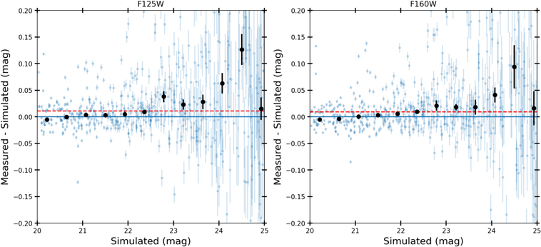
Figure 21. Measured fake star magnitudes minus simulated magnitudes as a function of mag for F125W (left) and F160W (right), with the median bias shown in red. We find just 1 mmag biases for sources brighter than 22 mag and ∼1% median biases overall, likely due to centroiding errors that are corrected in the real data thanks to multiple observational epochs.
Download figure:
Standard image High-resolution imageAppendix B: Coordinates and Photometric Measurements of RAISIN SNe
Table 6 contains coordinates and HST photometry for the RAISIN sample. Optical light curves and spectra are provided in the online data release accompanying this paper at https://doi.org/10.5281/zenodo.6349657.
Table 6. RAISIN Photometry
| SNID | MJD | filter |

|

| mhost | σhost | σc |

| σtmpl |
|---|---|---|---|---|---|---|---|---|---|
| (mag) | (mag) | (mag) | (mag) | (″) | (mag) | (mag) | |||
| PS1-480464 | 56370 | F160W | 24.017 ± 0.080 | 0.073 | 23.304 | 0.033 | 0.006 | 0.000 | 0.000 |
| PS1-480464 | 56370 | F125W | 22.437 ± 0.039 | 0.022 | 23.459 | 0.033 | 0.006 | 0.009 | 0.005 |
| PS1-480464 | 56362 | F160W | 24.333 ± 0.114 | 0.109 | 23.304 | 0.033 | 0.006 | 0.000 | 0.000 |
| PS1-480464 | 56362 | F125W | 22.726 ± 0.047 | 0.033 | 23.459 | 0.033 | 0.006 | 0.011 | 0.007 |
| PS1-480464 | 56357 | F160W | 24.253 ± 0.122 | 0.117 | 23.304 | 0.035 | 0.006 | 0.000 | 0.000 |
| PS1-480464 | 56357 | F125W | 22.921 ± 0.049 | 0.035 | 23.459 | 0.034 | 0.006 | 0.013 | 0.008 |
| PS1-450082 | 56265 | F125W | 22.834 ± 0.238 | 0.030 | 20.889 | 0.236 | 0.003 | 0.014 | 0.008 |
| PS1-450082 | 56265 | F160W | 24.573 ± 0.250 | 0.150 | 20.564 | 0.200 | 0.003 | 0.000 | 0.000 |
| PS1-450082 | 56272 | F125W | 22.505 ± 0.237 | 0.022 | 20.889 | 0.236 | 0.003 | 0.010 | 0.006 |
| PS1-450082 | 56278 | F160W | 24.469 ± 0.235 | 0.124 | 20.564 | 0.200 | 0.003 | 0.000 | 0.000 |
| PS1-450082 | 56278 | F125W | 22.339 ± 0.237 | 0.022 | 20.889 | 0.236 | 0.003 | 0.009 | 0.005 |
| PS1-450082 | 56272 | F160W | 24.606 ± 0.239 | 0.132 | 20.564 | 0.199 | 0.003 | 0.000 | 0.000 |
| PS1-540087 | 56528 | F125W | 22.873 ± 0.078 | 0.043 | 21.797 | 0.065 | 0.002 | 0.011 | 0.006 |
| PS1-540087 | 56536 | F160W | 24.962 ± 0.303 | 0.294 | 21.539 | 0.073 | 0.002 | 0.000 | 0.000 |
| PS1-540087 | 56536 | F125W | 23.002 ± 0.078 | 0.045 | 21.797 | 0.064 | 0.002 | 0.012 | 0.007 |
| PS1-540087 | 56528 | F160W | 23.748 ± 0.114 | 0.088 | 21.539 | 0.072 | 0.002 | 0.000 | 0.000 |
| PS1-540087 | 56523 | F160W | 23.394 ± 0.103 | 0.072 | 21.539 | 0.074 | 0.002 | 0.000 | 0.000 |
| PS1-540087 | 56523 | F125W | 22.657 ± 0.074 | 0.036 | 21.797 | 0.065 | 0.002 | 0.009 | 0.005 |
| PS1- 520188 | 56488 | F125W | 22.534 ± 0.035 | 0.027 | 26.192 | 0.021 | 0.001 | 0.022 | 0.013 |
| PS1-520188 | 56501 | F160W | 24.140 ± 0.075 | 0.071 | 26.190 | 0.024 | 0.001 | 0.000 | 0.000 |
| PS1-520188 | 56501 | F125W | 22.573 ± 0.034 | 0.026 | 26.192 | 0.022 | 0.001 | 0.023 | 0.014 |
| PS1-520188 | 56494 | F160W | 23.815 ± 0.048 | 0.041 | 26.190 | 0.025 | 0.001 | 0.000 | 0.000 |
| PS1-520188 | 56494 | F125W | 22.689 ± 0.034 | 0.026 | 26.192 | 0.021 | 0.001 | 0.026 | 0.015 |
| PS1-520188 | 56488 | F160W | 23.133 ± 0.037 | 0.028 | 26.190 | 0.024 | 0.001 | 0.000 | 0.000 |
| DES16E2cxw | 57715 | F125W | 22.771 ± 0.275 | 0.021 | 20.420 | 0.274 | 0.002 | 0.008 | 0.005 |
| DES16E2cxw | 57715 | F160W | 23.874 ± 0.200 | 0.072 | 20.203 | 0.187 | 0.002 | 0.000 | 0.000 |
| DES16E2cxw | 57723 | F125W | 22.691 ± 0.275 | 0.020 | 20.420 | 0.274 | 0.002 | 0.007 | 0.004 |
| DES16E2cxw | 57723 | F160W | 23.902 ± 0.204 | 0.082 | 20.203 | 0.187 | 0.002 | 0.000 | 0.000 |
| DES16E2cxw | 57730 | F125W | 22.455 ± 0.274 | 0.018 | 20.420 | 0.273 | 0.002 | 0.006 | 0.003 |
| DES16E2cxw | 57730 | F160W | 24.314 ± 0.213 | 0.102 | 20.203 | 0.187 | 0.002 | 0.000 | 0.000 |
| PS1-440005 | 56229 | F125W | 22.965 ± 0.071 | 0.033 | 21.715 | 0.063 | 0.007 | 0.014 | 0.008 |
| PS1-440005 | 56229 | F160W | 24.079 ± 0.127 | 0.090 | 21.387 | 0.090 | 0.007 | 0.000 | 0.000 |
| PS1-440005 | 56235 | F160W | 24.502 ± 0.159 | 0.131 | 21.387 | 0.090 | 0.007 | 0.000 | 0.000 |
| PS1-440005 | 56242 | F125W | 22.734 ± 0.070 | 0.031 | 21.715 | 0.063 | 0.007 | 0.011 | 0.007 |
| PS1-440005 | 56242 | F160W | 24.137 ± 0.119 | 0.078 | 21.387 | 0.090 | 0.007 | 0.000 | 0.000 |
| PS1-440005 | 56235 | F125W | 22.998 ± 0.075 | 0.042 | 21.715 | 0.063 | 0.007 | 0.014 | 0.008 |
| PS1-520062 | 56473 | F125W | 23.082 ± 0.077 | 0.033 | 21.979 | 0.069 | 0.002 | 0.016 | 0.009 |
| PS1-520062 | 56473 | F160W | 25.973 ± 0.315 | 0.310 | 21.769 | 0.056 | 0.002 | 0.000 | 0.000 |
| PS1-520062 | 56482 | F125W | 22.894 ± 0.074 | 0.030 | 21.979 | 0.068 | 0.002 | 0.013 | 0.008 |
| PS1-520062 | 56482 | F160W | 25.101 ± 0.197 | 0.189 | 21.769 | 0.056 | 0.002 | 0.000 | 0.000 |
| PS1-520062 | 56468 | F125W | 23.087 ± 0.080 | 0.040 | 21.979 | 0.069 | 0.002 | 0.016 | 0.009 |
| PS1-520062 | 56468 | F160W | 24.669 ± 0.100 | 0.084 | 21.769 | 0.054 | 0.002 | 0.000 | 0.000 |
| PS1-500100 | 56424 | F160W | 24.034 ± 0.076 | 0.072 | 25.917 | 0.024 | 0.002 | 0.000 | 0.000 |
| PS1- 500100 | 56424 | F125W | 22.806 ± 0.042 | 0.036 | 26.200 | 0.021 | 0.002 | 0.015 | 0.009 |
| PS1-500100 | 56416 | F160W | 24.521 ± 0.116 | 0.114 | 25.917 | 0.021 | 0.002 | 0.000 | 0.000 |
| PS1-500100 | 56411 | F125W | 23.141 ± 0.041 | 0.035 | 26.200 | 0.021 | 0.002 | 0.020 | 0.012 |
| PS1-500100 | 56411 | F160W | 24.920 ± 0.134 | 0.133 | 25.917 | 0.016 | 0.002 | 0.000 | 0.000 |
| PS1-500100 | 56416 | F125W | 22.959 ± 0.047 | 0.042 | 26.200 | 0.021 | 0.002 | 0.017 | 0.010 |
| PS1-500301 | 56418 | F125W | 23.058 ± 0.166 | 0.038 | 21.263 | 0.161 | 0.002 | 0.027 | 0.016 |
| PS1-500301 | 56431 | F160W | 23.823 ± 0.134 | 0.046 | 21.080 | 0.126 | 0.002 | 0.000 | 0.000 |
| PS1-500301 | 56431 | F125W | 22.813 ± 0.164 | 0.030 | 21.263 | 0.162 | 0.002 | 0.021 | 0.012 |
| PS1-500301 | 56423 | F160W | 23.995 ± 0.140 | 0.060 | 21.080 | 0.126 | 0.002 | 0.000 | 0.000 |
| PS1-500301 | 56423 | F125W | 22.956 ± 0.166 | 0.037 | 21.263 | 0.161 | 0.002 | 0.025 | 0.014 |
| PS1-500301 | 56418 | F160W | 24.027 ± 0.147 | 0.077 | 21.080 | 0.125 | 0.002 | 0.000 | 0.000 |
| PS1-470041 | 56333 | F160W | 23.018 ± 0.193 | 0.026 | 20.335 | 0.191 | 0.018 | 0.000 | 0.000 |
| PS1-470041 | 56333 | F125W | 22.488 ± 0.289 | 0.023 | 20.518 | 0.288 | 0.018 | 0.006 | 0.004 |
| PS1-470041 | 56325 | F160W | 23.109 ± 0.193 | 0.019 | 20.335 | 0.192 | 0.018 | 0.000 | 0.000 |
| PS1-470041 | 56325 | F125W | 22.632 ± 0.289 | 0.022 | 20.518 | 0.288 | 0.018 | 0.007 | 0.004 |
| PS1-470041 | 56320 | F160W | 23.964 ± 0.205 | 0.074 | 20.335 | 0.191 | 0.018 | 0.000 | 0.000 |
| PS1-470041 | 56320 | F125W | 23.121 ± 0.291 | 0.040 | 20.518 | 0.288 | 0.018 | 0.012 | 0.007 |
| PS1-470041 | 56395 | F125W | 24.080 ± 0.302 | 0.091 | 20.518 | 0.288 | 0.018 | 0.028 | 0.016 |
| PS1-470041 | 56395 | F160W | 23.642 ± 0.202 | 0.062 | 20.335 | 0.192 | 0.018 | 0.000 | 0.000 |
| PS1-480794 | 56368 | F125W | 23.284 ± 0.053 | 0.034 | 23.014 | 0.041 | 0.002 | 0.013 | 0.007 |
| PS1-480794 | 56361 | F160W | 24.189 ± 0.087 | 0.080 | 22.905 | 0.034 | 0.002 | 0.000 | 0.000 |
| PS1-480794 | 56361 | F125W | 23.064 ± 0.058 | 0.040 | 23.014 | 0.042 | 0.002 | 0.010 | 0.006 |
| PS1-480794 | 56355 | F160W | 23.786 ± 0.060 | 0.049 | 22.905 | 0.035 | 0.002 | 0.000 | 0.000 |
| PS1-480794 | 56368 | F160W | 24.635 ± 0.165 | 0.161 | 22.905 | 0.036 | 0.002 | 0.000 | 0.000 |
| PS1-480794 | 56355 | F125W | 22.887 ± 0.054 | 0.034 | 23.014 | 0.042 | 0.002 | 0.009 | 0.005 |
| PS1- 490521 | 56396 | F160W | 23.974 ± 0.084 | 0.066 | 22.011 | 0.052 | 0.001 | 0.000 | 0.000 |
| PS1-490521 | 56396 | F125W | 22.979 ± 0.080 | 0.032 | 22.226 | 0.073 | 0.001 | 0.005 | 0.003 |
| PS1-490521 | 56389 | F160W | 24.295 ± 0.097 | 0.082 | 22.011 | 0.052 | 0.001 | 0.000 | 0.000 |
| PS1-490521 | 56389 | F125W | 23.089 ± 0.079 | 0.027 | 22.226 | 0.074 | 0.001 | 0.006 | 0.003 |
| PS1-490521 | 56383 | F125W | 23.197 ± 0.077 | 0.021 | 22.226 | 0.074 | 0.001 | 0.007 | 0.004 |
| PS1-490521 | 56383 | F160W | 24.300 ± 0.081 | 0.062 | 22.011 | 0.052 | 0.001 | 0.000 | 0.000 |
| PS1-470110 | 56326 | F160W | 24.419 ± 0.079 | 0.074 | 23.854 | 0.027 | 0.007 | 0.038 | 0.022 |
| PS1-470110 | 56321 | F125W | 22.968 ± 0.054 | 0.038 | 23.948 | 0.038 | 0.007 | 0.022 | 0.013 |
| PS1-470110 | 56321 | F160W | 23.979 ± 0.072 | 0.067 | 23.854 | 0.026 | 0.007 | 0.025 | 0.014 |
| PS1-470110 | 56326 | F125W | 23.133 ± 0.058 | 0.045 | 23.948 | 0.037 | 0.007 | 0.026 | 0.015 |
| PS1-470110 | 56334 | F160W | 24.592 ± 0.108 | 0.105 | 23.854 | 0.025 | 0.007 | 0.044 | 0.026 |
| PS1-470110 | 56334 | F125W | 23.198 ± 0.053 | 0.038 | 23.948 | 0.037 | 0.007 | 0.027 | 0.016 |
| DES16E2clk | 57707 | F125W | 23.375 ± 0.058 | 0.036 | 22.835 | 0.046 | 0.001 | 0.010 | 0.006 |
| DES16E2clk | 57712 | F160W | 24.640 ± 0.147 | 0.141 | 22.709 | 0.042 | 0.001 | 0.014 | 0.008 |
| DES16E2clk | 57719 | F125W | 23.310 ± 0.054 | 0.028 | 22.835 | 0.046 | 0.001 | 0.009 | 0.005 |
| DES16E2clk | 57719 | F160W | 24.514 ± 0.117 | 0.111 | 22.709 | 0.037 | 0.001 | 0.012 | 0.007 |
| DES16E2clk | 57707 | F160W | 24.873 ± 0.195 | 0.191 | 22.709 | 0.039 | 0.001 | 0.017 | 0.010 |
| DES16E2clk | 57712 | F125W | 23.364 ± 0.053 | 0.028 | 22.835 | 0.046 | 0.001 | 0.010 | 0.006 |
| DES16C2cva | 57729 | F160W | 24.126 ± 0.074 | 0.054 | 22.106 | 0.051 | 0.015 | 0.007 | 0.004 |
| DES16C2cva | 57721 | F160W | 24.586 ± 0.081 | 0.063 | 22.106 | 0.051 | 0.015 | 0.010 | 0.006 |
| DES16C2cva | 57714 | F160W | 24.798 ± 0.090 | 0.074 | 22.106 | 0.051 | 0.015 | 0.012 | 0.007 |
| DES15X2kvt | 57321 | F160W | 24.926 ± 0.166 | 0.162 | 23.081 | 0.036 | 0.002 | 0.010 | 0.006 |
| DES15X2kvt | 57327 | F160W | 24.722 ± 0.131 | 0.126 | 23.081 | 0.036 | 0.002 | 0.008 | 0.005 |
| DES15X2kvt | 57337 | F160W | 24.081 ± 0.102 | 0.096 | 23.081 | 0.034 | 0.002 | 0.005 | 0.003 |
| PS1-450339 | 56282 | F125W | 23.432 ± 0.070 | 0.063 | 24.447 | 0.031 | 0.001 | 0.010 | 0.006 |
| PS1- 450339 | 56266 | F125W | 23.527 ± 0.060 | 0.052 | 24.447 | 0.030 | 0.001 | 0.011 | 0.007 |
| PS1-450339 | 56266 | F160W | 24.604 ± 0.112 | 0.109 | 24.387 | 0.026 | 0.001 | 0.008 | 0.005 |
| PS1-450339 | 56272 | F125W | 23.541 ± 0.059 | 0.051 | 24.447 | 0.030 | 0.001 | 0.011 | 0.007 |
| PS1-450339 | 56282 | F160W | 24.293 ± 0.098 | 0.094 | 24.387 | 0.028 | 0.001 | 0.006 | 0.004 |
| PS1-450339 | 56272 | F160W | 24.665 ± 0.140 | 0.137 | 24.387 | 0.029 | 0.001 | 0.008 | 0.005 |
| DES15E2nlz | 57404 | F160W | 24.366 ± 0.058 | 0.053 | 25.538 | 0.023 | 0.007 | 0.025 | 0.014 |
| DES15E2nlz | 57396 | F160W | 24.641 ± 0.065 | 0.061 | 25.538 | 0.022 | 0.007 | 0.032 | 0.018 |
| DES15E2nlz | 57390 | F160W | 24.604 ± 0.086 | 0.083 | 25.538 | 0.022 | 0.007 | 0.031 | 0.018 |
| PS1-530251 | 56515 | F125W | 23.766 ± 0.092 | 0.087 | 25.038 | 0.030 | 0.002 | 0.015 | 0.009 |
| PS1-530251 | 56508 | F160W | 24.884 ± 0.185 | 0.183 | 25.120 | 0.027 | 0.002 | 0.012 | 0.007 |
| PS1-530251 | 56508 | F125W | 23.830 ± 0.100 | 0.096 | 25.038 | 0.028 | 0.002 | 0.016 | 0.009 |
| PS1-530251 | 56502 | F160W | 24.541 ± 0.141 | 0.139 | 25.120 | 0.024 | 0.002 | 0.009 | 0.005 |
| PS1-530251 | 56502 | F125W | 23.613 ± 0.068 | 0.062 | 25.038 | 0.030 | 0.002 | 0.013 | 0.008 |
| PS1-530251 | 56515 | F160W | 24.662 ± 0.150 | 0.148 | 25.120 | 0.024 | 0.002 | 0.010 | 0.006 |
| PS1-550202 | 56600 | F160W | 24.425 ± 0.070 | 0.057 | 22.584 | 0.042 | 0.002 | 0.014 | 0.008 |
| PS1-550202 | 56586 | F160W | 24.761 ± 0.113 | 0.105 | 22.584 | 0.042 | 0.002 | 0.018 | 0.011 |
| PS1-550202 | 56593 | F125W | 23.616 ± 0.069 | 0.043 | 22.692 | 0.054 | 0.002 | 0.023 | 0.013 |
| PS1-550202 | 56593 | F160W | 24.661 ± 0.086 | 0.075 | 22.584 | 0.042 | 0.002 | 0.017 | 0.010 |
| PS1-550202 | 56610 | F160W | 23.898 ± 0.052 | 0.030 | 22.584 | 0.042 | 0.002 | 0.008 | 0.005 |
| PS1-550202 | 56586 | F125W | 23.520 ± 0.064 | 0.035 | 22.692 | 0.054 | 0.002 | 0.021 | 0.012 |
| DES15C1nhv | 57401 | F160W | 23.655 ± 0.045 | 0.036 | 24.039 | 0.026 | 0.001 | 0.025 | 0.015 |
| DES15C1nhv | 57387 | F160W | 24.035 ± 0.051 | 0.043 | 24.039 | 0.027 | 0.001 | 0.036 | 0.021 |
| DES15C1nhv | 57394 | F160W | 23.955 ± 0.045 | 0.036 | 24.039 | 0.026 | 0.001 | 0.034 | 0.020 |
| PS1-490037 | 56390 | F125W | 23.568 ± 0.119 | 0.095 | 22.154 | 0.073 | 0.000 | 0.028 | 0.017 |
| PS1-490037 | 56376 | F125W | 23.161 ± 0.092 | 0.057 | 22.154 | 0.072 | 0.000 | 0.019 | 0.011 |
| PS1- 490037 | 56376 | F160W | 24.209 ± 0.153 | 0.144 | 21.858 | 0.052 | 0.000 | 0.014 | 0.008 |
| PS1-490037 | 56381 | F125W | 23.358 ± 0.092 | 0.057 | 22.154 | 0.072 | 0.000 | 0.023 | 0.013 |
| PS1-490037 | 56390 | F160W | 24.769 ± 0.231 | 0.225 | 21.858 | 0.052 | 0.000 | 0.025 | 0.014 |
| PS1-490037 | 56381 | F160W | 24.450 ± 0.167 | 0.159 | 21.858 | 0.051 | 0.000 | 0.018 | 0.011 |
| DES16E2cqq | 57731 | F160W | 24.139 ± 0.050 | 0.037 | 23.247 | 0.034 | 0.002 | 0.006 | 0.003 |
| DES16E2cqq | 57721 | F160W | 24.552 ± 0.051 | 0.039 | 23.247 | 0.033 | 0.002 | 0.008 | 0.005 |
| DES16E2cqq | 57714 | F160W | 24.897 ± 0.082 | 0.075 | 23.247 | 0.033 | 0.002 | 0.011 | 0.007 |
| PS1-440236 | 56242 | F160W | 24.150 ± 0.065 | 0.062 | 28.020 | 0.020 | 0.000 | 0.009 | 0.005 |
| PS1-440236 | 56234 | F125W | 23.580 ± 0.042 | 0.037 | 29.261 | 0.021 | 0.000 | 0.019 | 0.011 |
| PS1-440236 | 56234 | F160W | 24.640 ± 0.094 | 0.092 | 28.020 | 0.019 | 0.000 | 0.014 | 0.008 |
| PS1-440236 | 56242 | F125W | 23.471 ± 0.036 | 0.030 | 29.261 | 0.021 | 0.000 | 0.018 | 0.010 |
| PS1-440236 | 56229 | F160W | 24.872 ± 0.129 | 0.127 | 28.020 | 0.023 | 0.000 | 0.017 | 0.010 |
| PS1-440236 | 56229 | F125W | 23.659 ± 0.041 | 0.034 | 29.261 | 0.022 | 0.000 | 0.021 | 0.012 |
| PS1-470240 | 56333 | F160W | 24.507 ± 0.076 | 0.076 | ⋯ | ⋯ | 0.001 | ⋯ | ⋯ |
| PS1-470240 | 56333 | F125W | 23.638 ± 0.039 | 0.039 | ⋯ | ⋯ | 0.001 | ⋯ | ⋯ |
| PS1-470240 | 56350 | F125W | 23.469 ± 0.040 | 0.040 | ⋯ | ⋯ | 0.001 | ⋯ | ⋯ |
| PS1-470240 | 56350 | F160W | 23.779 ± 0.045 | 0.045 | ⋯ | ⋯ | 0.001 | ⋯ | ⋯ |
| PS1-470240 | 56325 | F160W | 24.662 ± 0.047 | 0.047 | ⋯ | ⋯ | 0.001 | ⋯ | ⋯ |
| PS1-470240 | 56325 | F125W | 23.659 ± 0.055 | 0.055 | ⋯ | ⋯ | 0.001 | ⋯ | ⋯ |
| PS1-470240 | 56320 | F160W | 24.561 ± 0.066 | 0.066 | ⋯ | ⋯ | 0.001 | ⋯ | ⋯ |
| PS1-470240 | 56320 | F125W | 23.522 ± 0.037 | 0.037 | ⋯ | ⋯ | 0.001 | ⋯ | ⋯ |
| DES16X1cpf | 57708 | F160W | 23.703 ± 0.201 | 0.034 | 20.531 | 0.198 | 0.004 | 0.010 | 0.006 |
| DES16X1cpf | 57716 | F160W | 23.592 ± 0.200 | 0.025 | 20.531 | 0.199 | 0.004 | 0.009 | 0.005 |
| DES16X1cpf | 57723 | F160W | 23.424 ± 0.200 | 0.026 | 20.531 | 0.198 | 0.004 | 0.008 | 0.005 |
| DES15E2mhy | 57357 | F160W | 24.070 ± 0.072 | 0.049 | 21.922 | 0.053 | 0.002 | 0.027 | 0.016 |
| DES15E2mhy | 57373 | F160W | 24.293 ± 0.078 | 0.057 | 21.922 | 0.053 | 0.002 | 0.033 | 0.020 |
| DES15E2mhy | 57363 | F160W | 24.378 ± 0.078 | 0.058 | 21.922 | 0.052 | 0.002 | 0.036 | 0.021 |
| PS1- 560027 | 56601 | F160W | 24.147 ± 0.082 | 0.079 | 25.655 | 0.022 | 0.001 | 0.007 | 0.004 |
| PS1-560027 | 56593 | F125W | 23.494 ± 0.041 | 0.036 | 26.393 | 0.019 | 0.001 | 0.014 | 0.008 |
| PS1-560027 | 56593 | F160W | 24.495 ± 0.090 | 0.087 | 25.655 | 0.023 | 0.001 | 0.010 | 0.006 |
| PS1-560027 | 56611 | F160W | 23.800 ± 0.049 | 0.044 | 25.655 | 0.022 | 0.001 | 0.005 | 0.003 |
| PS1-560027 | 56587 | F125W | 23.509 ± 0.043 | 0.038 | 26.393 | 0.020 | 0.001 | 0.015 | 0.009 |
| PS1-560027 | 56587 | F160W | 24.784 ± 0.124 | 0.122 | 25.655 | 0.022 | 0.001 | 0.013 | 0.008 |
| DES16E1dcx | 57715 | F160W | 24.177 ± 0.135 | 0.124 | 21.997 | 0.053 | 0.002 | 0.004 | 0.002 |
| DES16E1dcx | 57730 | F160W | 24.218 ± 0.076 | 0.055 | 21.997 | 0.052 | 0.002 | 0.004 | 0.003 |
| DES16E1dcx | 57730 | F125W | 23.525 ± 0.083 | 0.047 | 22.416 | 0.068 | 0.002 | 0.007 | 0.004 |
| DES16E1dcx | 57722 | F160W | 24.594 ± 0.143 | 0.133 | 21.997 | 0.053 | 0.002 | 0.006 | 0.004 |
| DES16E1dcx | 57722 | F125W | 23.733 ± 0.084 | 0.049 | 22.416 | 0.068 | 0.002 | 0.009 | 0.005 |
| DES16E1dcx | 57715 | F125W | 23.487 ± 0.083 | 0.048 | 22.416 | 0.068 | 0.002 | 0.007 | 0.004 |
| DES15X2nkz | 57384 | F160W | 24.529 ± 0.074 | 0.069 | 23.892 | 0.029 | 0.003 | 0.032 | 0.019 |
| DES15X2nkz | 57391 | F160W | 24.853 ± 0.108 | 0.104 | 23.892 | 0.029 | 0.003 | 0.042 | 0.025 |
| DES15X2nkz | 57399 | F160W | 24.630 ± 0.082 | 0.078 | 23.892 | 0.028 | 0.003 | 0.035 | 0.020 |
| DES16S1bno | 57686 | F160W | 24.823 ± 0.084 | 0.080 | 26.342 | 0.026 | 0.001 | 0.009 | 0.006 |
| DES16S1bno | 57693 | F160W | 24.409 ± 0.074 | 0.070 | 26.342 | 0.024 | 0.001 | 0.007 | 0.004 |
| DES16S1bno | 57701 | F160W | 24.134 ± 0.054 | 0.048 | 26.342 | 0.025 | 0.001 | 0.005 | 0.003 |
| PS1-540118 | 56528 | F160W | 24.572 ± 0.097 | 0.091 | 23.302 | 0.033 | 0.001 | 0.017 | 0.010 |
| PS1-540118 | 56536 | F160W | 24.721 ± 0.099 | 0.093 | 23.302 | 0.034 | 0.001 | 0.020 | 0.012 |
| PS1-540118 | 56523 | F160W | 24.262 ± 0.077 | 0.070 | 23.302 | 0.032 | 0.001 | 0.013 | 0.008 |
| PS1-560054 | 56603 | F125W | 23.667 ± 0.073 | 0.063 | 24.039 | 0.038 | 0.001 | 0.024 | 0.014 |
| PS1-560054 | 56587 | F160W | 24.522 ± 0.109 | 0.106 | 23.871 | 0.025 | 0.001 | 0.017 | 0.010 |
| PS1-560054 | 56587 | F125W | 23.444 ± 0.066 | 0.055 | 24.039 | 0.036 | 0.001 | 0.019 | 0.011 |
| PS1-560054 | 56592 | F160W | 24.831 ± 0.192 | 0.190 | 23.871 | 0.028 | 0.001 | 0.022 | 0.013 |
| PS1- 560054 | 56603 | F160W | 24.432 ± 0.116 | 0.112 | 23.871 | 0.030 | 0.001 | 0.015 | 0.009 |
| PS1-560054 | 56592 | F125W | 23.726 ± 0.102 | 0.095 | 24.039 | 0.037 | 0.001 | 0.025 | 0.015 |
| DES16S2afz | 57657 | F160W | 24.244 ± 0.065 | 0.052 | 22.778 | 0.039 | 0.016 | 0.005 | 0.003 |
| DES16S2afz | 57663 | F160W | 24.420 ± 0.085 | 0.076 | 22.778 | 0.038 | 0.016 | 0.007 | 0.004 |
| DES16S2afz | 57671 | F160W | 24.296 ± 0.072 | 0.061 | 22.778 | 0.038 | 0.016 | 0.006 | 0.003 |
| DES16E2rd | 57657 | F160W | 23.980 ± 0.195 | 0.074 | 19.559 | 0.180 | 0.007 | 0.030 | 0.018 |
| DES16E2rd | 57663 | F160W | 24.049 ± 0.200 | 0.087 | 19.559 | 0.180 | 0.007 | 0.032 | 0.019 |
| DES16E2rd | 57671 | F160W | 23.632 ± 0.191 | 0.064 | 19.559 | 0.180 | 0.007 | 0.021 | 0.012 |
| DES16X3zd | 57657 | F160W | 24.558 ± 0.124 | 0.120 | 23.247 | 0.031 | 0.001 | 0.018 | 0.010 |
| DES16X3zd | 57663 | F160W | 24.546 ± 0.102 | 0.098 | 23.247 | 0.032 | 0.001 | 0.018 | 0.010 |
| DES16X3zd | 57672 | F160W | 24.240 ± 0.113 | 0.108 | 23.247 | 0.033 | 0.001 | 0.013 | 0.008 |
| PS1-510457 | 56457 | F160W | 25.043 ± 0.112 | 0.098 | 21.964 | 0.054 | 0.002 | 0.033 | 0.019 |
| PS1-510457 | 56444 | F160W | 25.221 ± 0.121 | 0.108 | 21.964 | 0.054 | 0.002 | 0.039 | 0.023 |
| PS1-510457 | 56439 | F160W | 25.086 ± 0.088 | 0.071 | 21.964 | 0.053 | 0.002 | 0.034 | 0.020 |
| DES16S1agd | 57672 | F160W | 24.285 ± 0.063 | 0.051 | 22.833 | 0.037 | 0.003 | 0.009 | 0.005 |
| DES16S1agd | 57657 | F160W | 24.565 ± 0.085 | 0.076 | 22.833 | 0.038 | 0.003 | 0.011 | 0.007 |
| DES16S1agd | 57663 | F160W | 24.501 ± 0.104 | 0.098 | 22.833 | 0.035 | 0.003 | 0.011 | 0.006 |
| DES15C3odz | 57429 | F160W | 24.508 ± 0.065 | 0.061 | 25.733 | 0.022 | 0.007 | 0.021 | 0.012 |
| DES15C3odz | 57421 | F160W | 25.022 ± 0.094 | 0.091 | 25.733 | 0.023 | 0.007 | 0.033 | 0.019 |
| DES15C3odz | 57414 | F160W | 25.291 ± 0.136 | 0.134 | 25.733 | 0.023 | 0.007 | 0.042 | 0.025 |
| PS1-520107 | 56473 | F160W | 24.132 ± 0.055 | 0.048 | 23.998 | 0.027 | 0.001 | 0.036 | 0.021 |
| PS1-520107 | 56482 | F160W | 24.114 ± 0.058 | 0.051 | 23.998 | 0.027 | 0.001 | 0.035 | 0.020 |
| PS1-520107 | 56468 | F160W | 24.064 ± 0.049 | 0.041 | 23.998 | 0.027 | 0.001 | 0.034 | 0.020 |
| DES16C1cim | 57721 | F160W | 24.318 ± 0.060 | 0.050 | 23.086 | 0.033 | 0.002 | 0.007 | 0.004 |
| DES16C1cim | 57712 | F160W | 24.527 ± 0.063 | 0.053 | 23.086 | 0.034 | 0.002 | 0.008 | 0.005 |
| DES16C1cim | 57706 | F160W | 24.772 ± 0.095 | 0.088 | 23.086 | 0.036 | 0.002 | 0.010 | 0.006 |
| DES16C3cmy | 57706 | F160W | 24.541 ± 0.068 | 0.064 | 25.646 | 0.023 | 0.001 | 0.010 | 0.006 |
| DES16C3cmy | 57720 | F160W | 24.492 ± 0.061 | 0.057 | 25.646 | 0.022 | 0.001 | 0.010 | 0.006 |
| DES16C3cmy | 57712 | F160W | 24.743 ± 0.075 | 0.071 | 25.646 | 0.024 | 0.001 | 0.012 | 0.007 |
| DES15E2uc | 57293 | F160W | 24.889 ± 0.081 | 0.075 | 23.465 | 0.030 | 0.016 | 0.029 | 0.017 |
| DES15E2uc | 57299 | F160W | 24.614 ± 0.082 | 0.075 | 23.465 | 0.033 | 0.016 | 0.022 | 0.013 |
| DES15E2uc | 57309 | F160W | 24.396 ± 0.060 | 0.051 | 23.465 | 0.031 | 0.016 | 0.018 | 0.011 |
| DES15X2mey | 57357 | F160W | 24.556 ± 0.092 | 0.086 | 23.068 | 0.032 | 0.001 | 0.029 | 0.017 |
| DES15X2mey | 57365 | F160W | 24.722 ± 0.092 | 0.086 | 23.068 | 0.032 | 0.001 | 0.034 | 0.020 |
| DES15X2mey | 57374 | F160W | 24.525 ± 0.083 | 0.075 | 23.068 | 0.035 | 0.001 | 0.029 | 0.017 |
| DES16X3cry | 57713 | F125W | 24.019 ± 0.043 | 0.026 | 24.218 | 0.034 | 0.001 | 0.007 | 0.004 |
| DES16X3cry | 57720 | F125W | 24.500 ± 0.051 | 0.037 | 24.218 | 0.035 | 0.001 | 0.011 | 0.006 |
| DES16X3cry | 57720 | F160W | 24.626 ± 0.054 | 0.046 | 24.015 | 0.028 | 0.001 | 0.007 | 0.004 |
| DES16X3cry | 57728 | F125W | 24.455 ± 0.064 | 0.054 | 24.218 | 0.034 | 0.001 | 0.011 | 0.006 |
| DES16X3cry | 57728 | F160W | 24.349 ± 0.080 | 0.076 | 24.015 | 0.025 | 0.001 | 0.006 | 0.003 |
Appendix C: Simulating the RAISIN Sample
Here we describe our simulations of the RAISIN sample. These simulations rely on an optical selection function that was determined for the PS1 and DES analyses (Scolnic et al. 2018; Kessler et al. 2019). We modeled the sample under the assumption that the RAISIN SNe were selected in an unbiased way from the subset of Pan-STARRS and DES SNe with spectroscopic classifications, and the typical S/N of the RAISIN optical light curves compared to the full PS1/DES spectroscopic samples shows this to be a reasonable approximation. Though RAISIN targeted SNe in specific redshift ranges, those redshift ranges—0.25 < z < 0.45 for RAISIN1 and 0.4 < z < 0.6 for RAISIN2—were within one standard deviation of the mean redshifts of the PS1 and DES SN spectroscopic surveys. Therefore, much of the necessary work for building these simulations for RAISIN was already undertaken by the MDS and DES teams. The main difference for RAISIN is the use of a new SN model, SNooPy, with the new optical-to-NIR dispersion model discussed in Section 3.3. We implemented the SNooPy model in SNANA by using the Python-based SNooPy code to generate a grid of model realizations as a function of sBV and AV , which SNANA may then use for both simulations and light-curve fitting (Figure 6). We then added a module to the SNANA simulation engine containing the SNooPy dispersion model, which generates correlated-random band-to-band offsets to be applied to the simulated magnitudes; this results in simulated distance-dependent biases. Both the SNooPy models and the SNooPy dispersion model are publicly available in SNANA.
For the low-z simulations, we do not have sky noise and zero-point information for the original NIR observations. However, SNANA is able to estimate these quantities by using the magnitudes and uncertainties in the data themselves to create a “simulation library.” Other low-z survey characteristics and selection effects were modeled in the Pantheon analysis (Scolnic et al. 2018), and we use the magnitude-based SN detection efficiency determined in that work to simulate the low-z CSP sample here. For the high-z simulations, our simulation library is built from observations of the RAISIN SNe themselves, which allows us to simulate SNe at the specific redshifts of the RAISIN objects and control for possible differences between the mean survey observing conditions and the conditions during which the RAISIN SNe were observed.
Finally, we require that simulated distributions of x1 and c parameters for SALT2 are replaced by distributions of the stretch parameter sBV and the extinction AV . Even though the light curves in NIR bands are less sensitive to sBV and AV than those in optical bands, an NIR-only approach with the RAISIN data does not allow shape/color to be corrected for, and therefore the results will be very sensitive to sample-to-sample differences in these parameters and the optical selection effects that will bias the sample toward, e.g., high sBV and low AV . We therefore adapt the method of Scolnic & Kessler (2016) to determine the intrinsic sBV distribution for the low-z and high-z samples. The distribution of the sBV parameter is treated as an asymmetric Gaussian following Scolnic & Kessler (2016), and we estimate the sBV distribution by fitting sBV with our NIR data.
For AV
, our baseline analysis assumes that the mean intrinsic dust extinction is independent of redshift, but we vary this assumption in our systematic error budget. We simulate an exponential dust distribution with  mag, which we find is a good approximate match to the optical+NIR data in Figure 22 and matches nominal dust distributions from the SN rate analysis of Rodney et al. (2014). We also find that varying τ globally has a minimal impact on the redshift dependence of our predicted bias corrections. Our two AV
-related systematic uncertainty analysis variants reduce the AV
scale length first by 0.05 for both samples (a small additional uncertainty) and second by 0.05 for the low-z sample only.
mag, which we find is a good approximate match to the optical+NIR data in Figure 22 and matches nominal dust distributions from the SN rate analysis of Rodney et al. (2014). We also find that varying τ globally has a minimal impact on the redshift dependence of our predicted bias corrections. Our two AV
-related systematic uncertainty analysis variants reduce the AV
scale length first by 0.05 for both samples (a small additional uncertainty) and second by 0.05 for the low-z sample only.
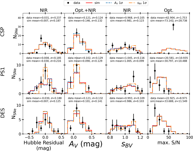
Figure 22. RAISIN simulations (red) compared to the data (black). Histograms of Hubble residuals, AV , sBV , and maximum S/N are shown for the CSP sample (top), the RAISIN1 sample (middle), and the RAISIN2 sample (bottom). Various combinations of data are used for comparison purposes as indicated above each column. Simulations after applying a 1σ shift to parameters of the AV and sBV distributions are shown in blue and orange, respectively. Some discrepancy in maximum S/N may be due to statistical fluctuation due to the small sample sizes in this analysis or uncertainty in the chosen SNooPy model.
Download figure:
Standard image High-resolution imageThe low-z sample from CSP used a galaxy-targeted approach to find SNe, which gives a sample of predominantly massive host galaxies and, as a result, increases the fraction of fast-declining SNe in the sample (Childress et al. 2013). For this reason we assume a priori that the low-z and RAISIN samples have different intrinsic stretch and color distributions. However, because the DES and MDS samples were selected in much the same way, and to avoid statistical noise, we assume that the intrinsic distributions of shape and color in these SN samples are the same. This is an approximation that is necessary owing to limited statistics, but the Scolnic & Kessler (2016) measurements of intrinsic population parameters in high-z samples show that this may be a good approximation. However, some evolution in population parameters (Nicolas et al. 2021) is expected, and larger samples at both high and low z in future analyses will allow constraints on this evolution, as well as a more robust determination of the stretch and color distributions themselves.
The resulting stretch and color distributions are shown in Figure 22. We find that both the sBV and AV distributions are statistically consistent between low- and high-z samples, albeit with relatively large uncertainties.
Finally, throughout this analysis we assume the default SNooPy total-to-selective extinction ratio of RV = 1.52 from Folatelli (2010, their Table 8), which reduces dispersion about the Hubble diagram compared to choosing the MW value of RV = 3.1 (Figure 18). The lower-than-expected value of RV may be due to the lack of an intrinsic color variation component of the SNooPy model (Thorp et al. 2021; Mandel et al. 2022) and the fact that extinction is allowed to be (unphysically) negative in this analysis. By using the CSP third data release and allowing SNooPy to fit for RV , we find that SNooPy gives a median RV ≃ 2, though unfortunately we find that the high-z RAISIN data are insufficient to constrain RV with SNooPy.
Because data at NIR wavelengths are a factor of ∼4−5 less sensitive to dust than the optical, distance error due to uncertainty in the value of RV is a sub-percent-level effect and will not be a significant component of the error budget in this analysis. We note that in the NIR fitting itself we treat AV as a constant, and therefore this effect will only change the distances in the bias correction stage.
The maximum S/N distributions are shown on the right side of Figure 22. Generally, the simulations expect slightly higher S/N than is observed in the data for high z. Because the larger PS1 and DES samples have a similar S/N near maximum light compared to the subset with RAISIN observations—nearly identical for PS1 and marginally higher S/N in the DES RAISIN subset—we choose not to modify the simulations here. The low-z S/N, on the other hand, has an unusual shape that we were unable to reproduce, perhaps due to small sample sizes; in the full SNooPy sample, before applying our selection cuts, we do not see the same concentration around a narrow range of S/N. In future, larger NIR samples it will be much easier to understand such artifacts in the data. We are unsure whether the NIR sample was selected in the same way as the rest of the CSP sample, but we assume that for this analysis; the simulations developed for past analyses are therefore sufficient given systematic uncertainties on the sBV and AV distributions. A low-z sample that selects NIR-observed SNe in an unbiased way is a key potential improvement for future cosmological analyses.
C.1. Distance Measurement Methodologies
Using the RAISIN simulations, we test the assumption that NIR-only distance measurements are most precise when sBV and AV are fixed to a constant value. From simulations, we measure a Hubble residual rms of 0.16 mag, slightly lower than the 0.19 mag measured from the real RAISIN data, when sBV and AV are fixed to a constant. When we attempt to use the NIR data alone to fit for AV , the Hubble residual rms increases to 0.28 mag, and when we fit for both sBV and AV , we measure an rms of 0.25 mag. However, when we use the NIR data alone to fit for sBV , we find that the rms is unchanged from the sBV fixed case; this may be because the simulated SNooPy model does not include the increase in scatter at later phases that we observe and discuss in Section 5.3. However, despite this modest discrepancy, both the simulations and real RAISIN data appear to show no benefit from fitting to AV and/or sBV with NIR data alone.
Appendix D: Host Mass Measurement
Host galaxy masses were reported by the CSP, DES, and MDS teams (Krisciunas et al. 2017; Jones et al. 2018b; Smith et al. 2020). However, to ensure consistency between all methods, we estimated the host galaxy masses of SNe in the RAISIN and low-z samples ourselves. For the low-z sample we used data from GALEX (Martin et al. 2005), Sloan Digital Sky Survey (SDSS) DR16 (Ahumada et al. 2020), PS1 DR2 (Flewelling et al. 2020), and the Two Micron All Sky Survey (2MASS; Skrutskie et al. 2006), while for the high-z sample we used only SDSS and PS1 as the other catalogs do not have sufficient depth for the faint, high-z RAISIN galaxies. For RAISIN2, we also used SN-free DES photometry from Wiseman et al. (2020). Finally, because PS1 3π images may be contaminated by SN light, we used MDS single-season template images for RAISIN1 SNe. The stacked images make it possible to detect  SN host galaxies with sufficient depth to measure masses on either side of the typical mass step location.
To find the host galaxy for each SN, we use SExtractor to determine the “directional light radius” between potential host galaxies and each SN (Sullivan et al. 2006; Gupta et al. 2016), a method that incorporates the size and orientation of each galaxy to determine which galaxy is the most likely host. Each most probable host was confirmed by eye, and thanks to HST imaging, we were able to determine which galaxies were the host without significant ambiguity. We then used SExtractor to measure the elliptical parameters of each galaxy in the r band, and then we used elliptical aperture photometry to measure the magnitudes of each galaxy in each available bandpass. The aperture size was chosen to extend slightly beyond the isophotal radius determined by SExtractor and was also extended to account for the increased PSF sizes of 2MASS and WISE. Any contamination by foreground stars was removed by using SExtractor to identify possible contaminants and masking those objects by setting the value of the pixels SExtractor deemed as belonging to those objects to the median value of the nearby pixels.
Once aperture photometry was measured, we used LePHARE (Arnouts & Ilbert 2011) with Bruzual & Charlot (2003) spectral templates and a Chabrier initial mass function (Chabrier 2003) to determine the stellar masses of each host galaxy. The templates include nine exponentially decreasing star formation histories in three metallicity bins, and we allow E(B − V) to vary from 0 to 0.4 in steps of 0.1 mag with a range of extinction laws. Uncertainties on these masses were estimated by Monte Carlo sampling of the photometry using the photometric uncertainties for each band and assuming a 1% error floor for bright galaxies. We note that mass estimation requires determining an absolute magnitude, making these mass estimates dependent on an assumed cosmology and the SN brightness residual. However, none of our mass estimates would change from <10 dex to >10 dex with modest adjustments in cosmological parameters; a 20% shift in w at a redshift of 0.6 would result in a systematic shift of just 0.03 dex relative to a low-z mass.
We compare these masses to estimates from Roman et al. (2018) for the low-z sample and Smith et al. (2020) for the high-z sample. Out of the 15 SNe with host masses in Roman et al. (2018), only one SN, SN 2004ey, disagrees with our high- versus low-mass designations. We do see a large median offset of −0.5 dex when subtracting the Roman et al. (2018) masses from ours, but we find that this is due to our addition of GALEX and 2MASS data; running LePHARE on our optical-only measurements gives a marginally significant median difference of +0.21 ± 0.08 dex for these SNe. For DES masses, we find a median difference of just 0.06 dex between our masses and those of Smith et al. (2020), with no disagreement between our high- and low-mass designations. Figure 8 shows histograms of the masses for CSP, RAISIN1, and RAISIN2 SNe; due to the targeted nature of the low-z CSP data, the CSP SNe are found in significantly more massive host galaxies.
For a given mass step location, with log (M*/M⊙) = 10 as the default, we assume that the uncertainties on the mass estimates are Gaussian and use these uncertainties to compute the probability that each SN has a mass greater than or less than the value at the step location. We then built a maximum likelihood, Gaussian mixture model that includes free parameters of the intrinsic dispersions for CSP, RAISIN1, and RAISIN2 (RAISIN2 has higher dispersion, as it uses one filter instead of two for most SNe); median Hubble residuals at low, medium, and high redshifts to remove sensitivity to the cosmological model; and a single mass step parameter. This procedure largely follows Jones et al. (2018a). We correct for the measured mass step in our data and apply two systematic uncertainties based on the value and location of the mass step as discussed in Section 3.7.4.
Appendix E: Distance Measurements for RAISIN and Low-z SNe
Table 7 contains NIR distances and optical+NIR stretch (sBV ) and AV measurements for RAISIN, computed using SNooPy and assuming an RV of 1.52.
Table 7. RAISIN Distances and Cuts
| ID | zHelio | Raw Distance | Rest-frame Bands | Bias Corr. |

| Avg. σphot | Cuts |
|---|---|---|---|---|---|---|---|
| (mag) | (mag) | (days) | (mag) | ||||
| PS1-480464 | 0.220 | 40.188 ± 0.033 | Y, J | 0.040 | 0.120 | 0.073 | ⋯ |
| PS1-450082 | 0.250 | ⋯ | ⋯ | ⋯ | 0.310 | 0.234 | bad host sub. |
| PS1-540087 | 0.275 | 40.621 ± 0.043 | Y, J | 0.073 | 0.350 | 0.145 | ⋯ |
| PS1-520188 | 0.280 | 40.350 ± 0.025 | Y, J | 0.073 | 0.050 | 0.040 | ⋯ |
| DES16E2cxw | 0.293 | ⋯ | ⋯ | ⋯ | 0.160 | 0.237 | bad host sub. |
| PS1-440005 | 0.306 | 40.771 ± 0.044 | Y, J | 0.049 | 0.410 | 0.102 | ⋯ |
| PS1-520062 | 0.308 | 41.168 ± 0.047 | Y, J | 0.049 | 0.290 | 0.128 | ⋯ |
| PS1-500100 | 0.310 | 40.991 ± 0.032 | Y, J | 0.046 | 0.390 | 0.069 | ⋯ |
| PS1-500301 | 0.325 | 40.727 ± 0.068 | Y, J | 0.038 | 0.420 | 0.145 | ⋯ |
| PS1-470041 | 0.331 | ⋯ | ⋯ | ⋯ | 0.120 | 0.242 | bad host sub. |
| PS1-480794 | 0.334 | ⋯ | ⋯ | ⋯ | 0.280 | 0.077 | high sBV |
| PS1-490521 | 0.340 | 40.982 ± 0.042 | Y, J | 0.033 | 0.430 | 0.082 | ⋯ |
| PS1-470110 | 0.346 | 41.128 ± 0.033 | Y, J | 0.035 | 0.190 | 0.074 | ⋯ |
| DES16E2clk | 0.367 | 41.340 ± 0.039 | Y, J | 0.041 | 0.240 | 0.103 | ⋯ |
| DES16C2cva | 0.403 | 41.699 ± 0.055 | Y | 0.019 | 0.330 | 0.080 | ⋯ |
| DES15X2kvt | 0.404 | 41.741 ± 0.078 | Y | 0.019 | 0.710 | 0.132 | ⋯ |
| PS1-450339 | 0.410 | 41.577 ± 0.034 | i, Y | 0.022 | 0.450 | 0.082 | ⋯ |
| PS1-530251 | 0.413 | 41.720 ± 0.045 | i, Y | 0.024 | 0.500 | 0.120 | ⋯ |
| DES15E2nlz | 0.410 | 41.715 ± 0.047 | Y | 0.021 | 0.390 | 0.066 | ⋯ |
| DES15C1nhv | 0.421 | ⋯ | ⋯ | ⋯ | 0.370 | 0.043 | Chauvenet |
| PS1-550202 | 0.422 | 41.698 ± 0.033 | i, Y | 0.025 | 0.800 | 0.073 | ⋯ |
| PS1-490037 | 0.422 | 41.500 ± 0.051 | i, Y | 0.025 | 0.370 | 0.147 | ⋯ |
| DES16E2cqq | 0.426 | 41.905 ± 0.042 | Y | 0.025 | 0.380 | 0.063 | ⋯ |
| PS1-470240 | 0.430 | 41.712 ± 0.024 | i, Y | 0.025 | 0.410 | 0.065 | ⋯ |
| DES16X1cpf | 0.436 | ⋯ | ⋯ | ⋯ | 0.380 | 0.201 | bad host sub. |
| PS1-440236 | 0.430 | 41.732 ± 0.024 | i, Y | 0.025 | 0.340 | 0.070 | ⋯ |
| DES15E2mhy | 0.439 | 41.528 ± 0.051 | Y | 0.029 | 0.340 | 0.079 | ⋯ |
| PS1- 560027 | 0.440 | 41.690 ± 0.027 | i, Y | 0.024 | 0.210 | 0.075 | ⋯ |
| DES16E1dcx | 0.453 | 41.679 ± 0.040 | i, Y | 0.029 | 0.340 | 0.105 | ⋯ |
| DES15X2nkz | 0.469 | 42.025 ± 0.056 | Y | 0.037 | 0.560 | 0.095 | ⋯ |
| DES16S1bno | 0.470 | 42.094 ± 0.046 | Y | 0.037 | 0.510 | 0.076 | ⋯ |
| PS1-540118 | 0.477 | 41.938 ± 0.058 | Y | 0.004 | 0.490 | 0.084 | ⋯ |
| PS1-560054 | 0.482 | 41.813 ± 0.040 | i, Y | 0.004 | 0.250 | 0.112 | ⋯ |
| DES16S2afz | 0.483 | 41.706 ± 0.051 | Y | 0.033 | 0.300 | 0.068 | ⋯ |
| DES16E2rd | 0.494 | ⋯ | ⋯ | ⋯ | 0.210 | 0.194 | bad host sub. |
| DES16X3zd | 0.495 | 41.905 ± 0.071 | Y | 0.030 | 0.220 | 0.103 | ⋯ |
| PS1-510457 | 0.502 | 42.625 ± 0.065 | Y | 0.004 | 0.890 | 0.106 | ⋯ |
| DES16S1agd | 0.504 | 41.925 ± 0.055 | Y | 0.031 | 0.490 | 0.086 | ⋯ |
| DES15C3odz | 0.508 | 42.538 ± 0.058 | Y | 0.031 | 0.320 | 0.094 | ⋯ |
| PS1-520107 | 0.519 | ⋯ | ⋯ | ⋯ | 1.960 | 0.049 | possible non-Ia |
| DES16C1cim | 0.531 | 42.282 ± 0.049 | Y | 0.024 | 0.570 | 0.070 | ⋯ |
| DES16C3cmy | 0.556 | 42.326 ± 0.048 | Y | 0.017 | 0.250 | 0.066 | ⋯ |
| DES15E2uc | 0.566 | 42.710 ± 0.048 | Y | 0.019 | 0.640 | 0.070 | ⋯ |
| DES15X2mey | 0.608 | 42.700 ± 0.058 | Y | 0.025 | 0.280 | 0.093 | ⋯ |
| DES16X3cry | 0.612 | 42.567 ± 0.028 | i, Y | 0.025 | 0.340 | 0.062 | ⋯ |
Note. Distance moduli from RAISIN SNe, calibrated to our best-fit H0 of 75.4 km s−1 Mpc−1. The “raw distance” (Column (3)) does not include the bias correction (Column (5)), which is added to the raw distance prior to cosmological parameter fitting. “Rest-frame Bands” (Column (4)) indicates the rest-frame SNooPy templates that were used to fit the RAISIN observations.
Download table as: ASCIITypeset image
Footnotes
- 25
- 26
SN 520107 has a large shape uncertainty, while SN 470240 has an unusually blue optical color but passes the NIR-based cuts in Table 1. The other three SNe, SN 480794, SN 540087, and SN 540118, appear to pass standard cosmology cuts and were used for the cosmological analysis in Jones et al. (2018b).
- 27
The NASA/IPAC Extragalactic Database (NED) is funded by the National Aeronautics and Space Administration and operated by the California Institute of Technology.
- 28
“Drizzling” refers to the process of linearly reconstructing an image from undersampled, dithered data (Fruchter & Hook 2002).
- 29
- 30
We adopt arbitrary values of sBV = 1 and AV = 0 for simplicity, as the bias correction stage will adjust the derived distances for the average sBV and AV of the data themselves. We have confirmed that adjusting the nominal value of these parameters in the distance fits does not change the scatter by more than ∼0.01 mag.
- 31
- 32
- 33
We note that this is also near the epoch in which the H-band spectral break occurs (Hsiao et al. 2013), but this would only affect our low-z data, where K-corrections are small.
- 34
- 35
- 36
This value is from the analysis variant in which Scolnic et al. (2018) do not apply bias corrections to the SN shape and color parameters and is the analysis version that is most comparable to our method here.
- 37
The data used in this analysis are published at https://doi.org/10.5281/zenodo.6349657.
- 38
- 39
- 40