Abstract
Recent precise measurements of primary and secondary cosmic-ray (CR) species in the teravolt rigidity domain have unveiled a bump in their spectra, located between 0.5 and 50 TV. We argue that a local shock may generate such a bump by increasing the rigidity of the preexisting CRs below 50 TV by a mere factor of ∼1.5. Reaccelerated particles below ∼0.5 TV are convected with the interstellar medium flow and do not reach the Sun, thus creating the bump. This single universal process is responsible for the observed spectra of all CR species in the rigidity range below 100 TV. We propose that one viable shock candidate is the Epsilon Eridani star at 3.2 pc from the Sun, which is well aligned with the direction of the local magnetic field. Other shocks, such as old supernova shells, may produce a similar effect. We provide a simple formula, Equation (9), that reproduces the spectra of all CR species with only two nonadjustable shock parameters, uniquely derived from the proton data. We show how our formalism predicts helium and carbon spectra and the B/C ratio.
Original content from this work may be used under the terms of the Creative Commons Attribution 4.0 licence. Any further distribution of this work must maintain attribution to the author(s) and the title of the work, journal citation and DOI.
1. Introduction: The Cosmic-Ray “Bump”
The last decade was marked by discoveries of new features in the spectra of cosmic-ray (CR) species. Unexpected breaks and variations in spectral indices are being unveiled with high confidence in the gigavolt–teravolt rigidity range that are deemed as well studied (Ahn et al. 2006; Panov et al. 2009; Ahn et al. 2010; Adriani et al. 2011; Yoon et al. 2011; Ackermann et al. 2014; Aguilar et al. 2015a, 2015b, 2017, 2018a, 2018b; Atkin et al. 2018; Grebenyuk et al. 2019a, 2019b; Atkin et al. 2019; Adriani et al. 2019; An et al. 2019; Aguilar et al. 2020, 2021). These features bear the signatures of CR acceleration processes and their propagation history.
First discovered was a flattening above  TV in rigidity in the CR proton and helium spectra (Ahn et al. 2006, 2010; Adriani et al. 2011), which triggered a slew of interpretations. However, with improved measurements of spectra of several primary (p, He, C, O, Ne, Mg, Si) and secondary
3
(Li, Be, B) species by AMS-02 (Aguilar et al. 2015a), only two interpretations remain feasible. These are (i) the intrinsic spectral break in the CR injection spectrum or populations of sources with soft and hard spectra, the so-called injection scenario (Vladimirov et al. 2012), and (ii) a break in the spectrum of interstellar turbulence translated into the break in the diffusion coefficient, the so-called propagation scenario (Blasi et al. 2012; Vladimirov et al. 2012; Aloisio et al. 2015). The latter has very few free parameters and is well supported (Boschini et al. 2020a, 2020b) by the AMS-02 data.
TV in rigidity in the CR proton and helium spectra (Ahn et al. 2006, 2010; Adriani et al. 2011), which triggered a slew of interpretations. However, with improved measurements of spectra of several primary (p, He, C, O, Ne, Mg, Si) and secondary
3
(Li, Be, B) species by AMS-02 (Aguilar et al. 2015a), only two interpretations remain feasible. These are (i) the intrinsic spectral break in the CR injection spectrum or populations of sources with soft and hard spectra, the so-called injection scenario (Vladimirov et al. 2012), and (ii) a break in the spectrum of interstellar turbulence translated into the break in the diffusion coefficient, the so-called propagation scenario (Blasi et al. 2012; Vladimirov et al. 2012; Aloisio et al. 2015). The latter has very few free parameters and is well supported (Boschini et al. 2020a, 2020b) by the AMS-02 data.
A turning point was the recent discovery of a steepening in the proton and helium spectra at  13 TV (Ahn et al. 2006; Atkin et al. 2018; Grebenyuk et al. 2019a; Atkin et al. 2019; Adriani et al. 2019; An et al. 2019), see parameterizations in Boschini et al. (2020b). Together with the lower rigidity break
  , the two features likely result from a single physical process that generates a bump in the CR spectrum between 0.5 and 50 TV. It peaks by a factor of 2.5–3 near ≈13 TV above the background CR spectrum extrapolated from low energies.
The discovery of the second break challenges conventional interpretations of the CR spectra outlined above. This finding also refutes earlier hypotheses of a contribution from a nearby CR accelerator, such as a supernova remnant (SNR), that accelerates the bump particles out of the interstellar medium (ISM; e.g., Fang et al. 2020; Yuan et al. 2020; Fornieri et al. 2021) because such a scenario implies no breaks in the secondary component (Vladimirov et al. 2012). Moreover, the unprecedented accuracy with which the sharp break at  in the CR spectrum is measured severely constrains its remote or global origins as they would lead to a smoother transition. The recently enhanced data accuracy even allows for the identification of the dominant turbulent regime through which these CRs propagate from the source to the observer. It was shown to be of Iroshnikov–Kraichnan type (Malkov & Moskalenko 2021, hereafter Paper I).
Another clue to the origin of the bump is the break in the spectra of secondary species that are also flattening above the first break ( ), similarly to the primaries, albeit with a different spectral index. It implies that the secondary species have already been present in the CR mixture that the bump is made of. This leads us to conclude that (i) the bump has to be made out of the preexisting CRs with all their primaries and secondaries that have spent millions of years in the Galaxy. Meanwhile, the sharpness of the breaks indicates that (ii) the bump is formed locally, a short time before we observed it.
In this paper, we argue that a single universal process is responsible for the observed spectra of all CR species in the rigidity range below 100 TV. We provide a simple formula, Equation (9), that reproduces the spectra of all CR species with only two shock parameters derived from a fit to the proton data. It then fully predicts the entire bump structure, including two break rigidities ( , Rbr″), two respective jumps in the spectral index, and two curvatures of the spectrum (sharpness) at the breaks—which would otherwise require six parameters for each CR species. We show how our formalism (Paper I) operates using the proton, helium, and carbon spectra, and the B/C ratio.
2. Local CR Reacceleration
An immediate consequence of the abovementioned reasoning is that the bump particles are background CRs reaccelerated inside of the Local Bubble. Estimates show that prospective sources should be within 3–10 pc of the Sun (Paper I). These sources can be of two kinds: pointlike and extended. We argue below that the difference between the two is significant. If the source is pointlike, it also has an elongated magnetic flux tube. The reaccelerated CRs propagate to the observer through it. Gradual lateral losses from the flux tube and the Iroshnikov–Kraichnan (IK; Iroshnikov 1964; Kraichnan 1965) MHD turbulence driven by the lateral pressure gradient of the reaccelerated CRs critically reshape their rigidity (10 TV bump) and angular spectra that fit to the most accurate recent data. By contrast, propagation of CRs from an extended source through a broad channel without significant lateral pressure gradient and IK turbulence would require additional assumptions to become consistent with those data.
The bow shocks and stellar wind termination shocks (TS) of nearby passing stars are obvious candidates of pointlike sources. However, most stars can be disqualified as they are not magnetically connected with the heliosphere. Surprisingly, we found a remarkable alignment of the local magnetic field with the Epsilon Eridani star at 3.2 pc from the Sun (Paper I). It also has an extensive 8000 au astrosphere and a 30 times higher than the solar mass-loss rate (Wood et al. 2002).
Nevertheless, simple estimates show that even a bow shock of such a significant size as ∼104 au might only marginally reaccelerate preexisting CRs by the required 1.5 factor to generate the bump. On the other hand, this can readily be done by a larger shock. Moreover, as any local shock is likely to be weak, CR species with initially steeper spectra experience a more significant reacceleration (see Equation (2) in the following section), which is consistent with observations of the secondaries. A particularly appealing source candidate is a sizable imploding shock in the local ISM, whose existence is supported observationally (Gry & Jenkins 2014), see discussion in Section 7.
Notwithstanding the advantage of a large shock, this source is also problematic, as we already mentioned. One serious contradiction comes from the angular distribution of CRs in the bump rigidity range. It rises sharply across the magnetic horizon and also has an enhanced field-aligned component (see Figure 11 in Abeysekara et al. 2019 and an extended discussion of available data in Paper I). These angular anomalies can be produced simultaneously if a pointlike source is located on one side of the flux tube connected to the solar system within several parsecs from the observer. CRs that diffusively propagate from the source along the flux tube also leak through the tube’s lateral boundary. Therefore, not all the CRs that passed the observer will return. The observer in the solar system will then see more CRs coming from the source than returning to it. The sharp contrast between these CR groups on the intensity map is critically associated with the IK spectrum of the scattering turbulence. The field-aligned component is not related to the CR losses but follows the solution of the complete Fokker–Plank transport problem, not limited by the diffusive approximation. It was shown (Malkov 2017) that the field-aligned component survives a longer propagation from the source (up to 5–7 particle mean free paths) than might have been expected.
Despite the rise at the CR pitch angle of 90° (magnetic horizon) and the field-aligned one-sided enhancement have different physical causes, their coexistence has been demonstrated (Paper I) by solving the proper CR propagation with lateral losses and the IK pitch-angle scattering. To our best knowledge, no other CR source and transport regime configuration fits the current data in the 1–100 TV range with dramatically shrunk statistical uncertainties (Aguilar et al. 2021, see also Figure 1 below).
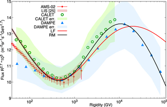
Figure 1. Proton rigidity spectrum from AMS-02, CALET, and DAMPE (Adriani et al. 2019; An et al. 2019; Aguilar et al. 2021). CALET and DAMPE data were modified to adjust for systematic differences between the three instruments, see text for details. The curves show the model calculations, Equation (9), for the cases of RL = ∞ (LF model) and a more realistic for high rigidities case of finite losses RL < ∞ (RM model). The model and input parameters are summarized in Tables 1 and 2.
Download figure:
Standard image High-resolution imageThe current data are so accurate and multifaceted (rigidity-, angular-, and chemical-composition spectra) that the reverse engineering of the 10 TV bump source and its propagation mode became possible without identifying any particular object presumably responsible for the bump. Still, the source is likely associated with a shock, whose parameters can be constrained, but the shock may remain invisible in the sky. In the Appendix, we provide a brief discussion of potentially qualified shocks.
The situation with a well described but unknown source is not entirely satisfactory, so we pursue two parallel approaches to improve it. One approach is to develop a generic shock reacceleration and CR propagation model along a magnetic flux tube pointing to the solar system. It depends on an unknown shock Mach number and its size-distance relation (Paper I). The model’s key advantage is that these parameters are uniquely derived from the best measured CR proton spectrum or its substitute. As the latter, we use synthetic data provided in Boschini et al. (2020b), i.e., a physically motivated local interstellar spectrum (LIS) of CR protons tuned to the data of different instruments with adjustments for the appropriate heliospheric modulation. As the slope and normalization of CR background LIS below the first break are now accurately derived (Boschini et al. 2020b), the model takes them as fixed input parameters. The turbulence index, found to be s = 3/2 (IK spectrum), critically determines the proton spectrum, yielding the precise spectral shape over four orders of magnitude in rigidity (Paper I). To further test our model, we turn to other species.
The second approach is to look at the Epsilon Eridani star as it is magnetically connected with our Sun and its distance is also in the right ballpark. However, as we noted, its bow shock is somewhat weak, making the reacceleration of CR of several tenths of teravolts problematic. This issue can be ameliorated considering that the bow shock and strong stellar wind TS coexist in the system, while the resulting bump spectrum is still primarily shaped during the CR propagation. We provide the corresponding formalism in the Appendix. In the following section, we review and extend to a broader geometrical setting a generic CR reacceleration and propagation model developed in Paper I. We now include the lateral particle losses in this model.
3. CR Reacceleration and Propagation Model
Only two parameters, constituting the bump amplitude, K, and rigidity, R0, suffice to predict the bump spectrum (Paper I) without particle losses from the flux tube. The reaccelerated CR density is elevated over the background by the factor

where γ is the spectral index of the background CRs and q > γ is that of the shock,  . Here r is the shock compression ratio, which we determine from the proton fit. The enhanced spectrum appears as a bump at some distance from the shock, as the reaccelerated CRs with lower rigidity do not reach the observer. There will also be a high-energy cutoff to the CR enhancement, associated with the particle losses from the flux tube and the limited shock size, which we also discuss later.
The background CR spectrum is f∞ ∝ R−γ , whereas the shock would accelerate the freshly injected thermal particles to R−q spectrum. However, as the shock is likely to be weak, that is q > γ ≈ 2.85 (for protons), the freshly accelerated CRs are submerged into the reaccelerated CR component. The CR density measured at a distance z from the shock is (Blandford & Ostriker 1978, Paper I):

where K is defined in Equation (1). The flux suppression exponent, Φ, is a path integral of particles propagating along the magnetic flux tube from the shock. One may distinguish between two cases of the relative motion of the shock and the observer, although the rigidity dependence of  is similar in both cases.
3.1. Propagation from Quasi-parallel Portions of Shock
If the shock normal makes an angle ϑBn with respect to the local magnetic field not too close to π/2, the CR distribution along the flux tube is determined by the balance between the CR convection with the flow and diffusion against it. In this case we have
Here  with ush being the shock velocity, and κ∥ is the parallel component of the diffusion tensor. The term
  describes lateral losses from the flux tube. The bump characteristic rigidity R0 is introduced by the relation
  . Here the power 1/2 corresponds to the IK turbulence. The parameter R0 combines the distance to the shock, z, velocity u, and the turbulence power that defines κ∥ in Equation (3). According to Paper I, R0 ∝ u2
z2/l⊥ where the characteristic scale of the CR pressure gradient across the flux tube is
. Here the power 1/2 corresponds to the IK turbulence. The parameter R0 combines the distance to the shock, z, velocity u, and the turbulence power that defines κ∥ in Equation (3). According to Paper I, R0 ∝ u2
z2/l⊥ where the characteristic scale of the CR pressure gradient across the flux tube is  /∂r. It sets the amplitude of magnetic perturbations driven by this gradient.
3.2. Propagation from Quasi-perpendicular Portions of Shock
In the case ϑBn ≈ π/2, partially satisfied in many curved shocks, we use the balance between the divergence of convective and diffusive CR fluxes in the shock frame, v · ∇F ∼ ∇∥ κ∥∇∥ F, which is consistent with Equations (2) and (3). Here F is the full-bump distribution related to f below. The CR diffusion proceeds primarily along the field, but the convective term is v · ∇F ≈ v ⊥ · ∇⊥ F, which we may write assuming the ISM wind being in the y-direction and the magnetic field in the z-direction. So we have v∂F/∂y ≈ κ∥∂2 F/∂z2, assuming that κ∥ is independent of z, for a simple illustration. The result will then have a similar to the former case exponential rigidity dependence,

Averaging over y, or rather over the radial coordinate inside the tube, r⊥, depends on the shock structure and CR propagation in the tube that controls the losses.
3.3. Lateral Losses of CRs
Lateral losses from the flux tube affect the high-rigidity end of the 10 TV bump, roughly between 10 and 50 TV. Our goal is to include them in a way applicable to different CR propagation regimes. Assuming a quasi-stationary distribution of reaccelerated CRs around a moving reaccelerator (e.g., a stellar bow shock) we balance the following channels of particle transport: convection along the field, two components of diffusion (parallel and perpendicular to the B-field), and the lateral losses.
If the convective transport is significant, it is convenient to use the bump component  in Equation (2) as a radially averaged part of its full distribution, F. Namely,
  , where a⊥ is the tube’s radius. The CR flux at r⊥ = a⊥ is
  Here κ⊥ is a cross-field component of the CR diffusion tensor. Particle losses from the flux tube depend on the distance from the source because the self-driven turbulence decreases with it. We use the following general relation between the two components of κ, (e.g., Drury 1983),
  , where κB
= crg
/3 is the Bohm diffusion, rg
is the Larmor radius, and
, where κB
= crg
/3 is the Bohm diffusion, rg
is the Larmor radius, and  is the spectral energy density of Alfvén waves evaluated at the resonant wavenumber
  . Alfvénic fluctuations inside the magnetic flux tube filled with reaccelerated CRs were shown to obey the IK law,
  (Paper I). In this case, κ⊥ ∝ R3/2, while κ∥ ∝ R1/2. It follows that for large R the path integral Φ in Equation (3) will be dominated by the second term, associated with lateral particle losses from the tube rather than their propagation along the field (the first term).
If the CR source velocity has a sizable component along the B-field, the lateral losses are balanced by the CR convection along the field. The diffusion in that direction is suppressed because of the self-driven IK turbulence. The CR flux from the magnetic tube,  , can be estimated by recognizing that the fluctuation level must drop at the tube’s edge, r⊥ = a⊥, as these fluctuations are driven by the excessive pressure of reaccelerated CRs inside the tube. Beyond this radius, CRs diffuse primarily along the field, since the level of the background ISM fluctuations is typically very small,
  at a scale of ∼ 1012–1013 cm (e.g., Achterberg et al. 1994). Hence, the scattering events resulting in the displacement of the particle guiding center are increasingly rare.
Upon reaching the edge of the flux tube particles almost instantaneously escape along the field, since  , notwithstanding the tube’s length being much larger than its lateral size. Under these conditions, the most plausible estimate for
  is ∼ − F/rg
. The CR flux through the lateral boundary of the tube scales with rigidity as ∼ κ⊥
F/rg
∝ R1/2
F. An equilibration of convective CR transport
v
· ∇F with these losses yields the following approximate relation: vz
∂fb
/∂z ≈ − κ⊥
fb
/rg
a⊥. Here vz
is the projection of the CR source velocity on the field direction. We thus obtain the following exponential decay of the CR density along the tube:
is ∼ − F/rg
. The CR flux through the lateral boundary of the tube scales with rigidity as ∼ κ⊥
F/rg
∝ R1/2
F. An equilibration of convective CR transport
v
· ∇F with these losses yields the following approximate relation: vz
∂fb
/∂z ≈ − κ⊥
fb
/rg
a⊥. Here vz
is the projection of the CR source velocity on the field direction. We thus obtain the following exponential decay of the CR density along the tube: ![${f}_{b}\propto \exp \left[-\sqrt{R/{R}_{L}}\right]$](https://content.cld.iop.org/journals/0004-637X/933/1/78/revision1/apjac7049ieqn24.gif) . Here RL
∝ 1/z2 is the rigidity cutoff associated with the lateral losses and z is the current distance to the source. The cutoff RL
also depends on the flow geometry and details of the CR escape that we discussed using only order of magnitude estimates above. Therefore, the path integral in Equation (3) at fixed z can be represented as
. Here RL
∝ 1/z2 is the rigidity cutoff associated with the lateral losses and z is the current distance to the source. The cutoff RL
also depends on the flow geometry and details of the CR escape that we discussed using only order of magnitude estimates above. Therefore, the path integral in Equation (3) at fixed z can be represented as

Fortunately, the same form of high-rigidity cutoff is applicable when the convective transport is negligible because of the flow geometry, i.e., vz ≈ 0. In this case, the lateral CR diffusion is balanced by that along the field

After substituting  , assuming that κ∥ is separable, i.e.,
  , and introducing a new variable
  /P, the last equation can be rewritten as follows:
This equation can be solved by separating the variables  :
:
where λ2 is a separation constant, which is also the spectral parameter of the problem for ϕ defined by the boundary conditions  and the requirement of the regularity of ϕ at r⊥ = 0 imposed on the second equation above. For
  , its solution is given by Bessel function, J0,
  , where μn
is its nth root,
, where μn
is its nth root,  , μ1 ≈ 2.5, μ2 ≈ 5.5,... In this case, the spectrum is λn
= μn
/a⊥
κ1. For
, μ1 ≈ 2.5, μ2 ≈ 5.5,... In this case, the spectrum is λn
= μn
/a⊥
κ1. For  , the eigenvalues
  also grow rapidly with n. Therefore, expanding the solution of Equation (7) in a series of eigenfunctions
  with coefficients
  ,
,
we can retain only the first term in the series at the observer position z. Note, that particle rigidity, R, enters Equation (6) as a parameter, so that the solution can be represented as follows:
The prefactor  is determined by the spectrum generated by the reaccelerator and the near-zone propagation. For example, considering the CR reacceleration at a generic shock wave, C1 includes the background CR spectrum (f∞ in Equation (2)) and the first term in Equation (3) or Equation (4). The choice between the two depends on the accelerator’s motion relative to the observer and the ambient B-field, as addressed earlier in this section. In either case, the exponential dependence on rigidity is in the form given by the first term in Equation (5). Nevertheless, different expressions for the CR bump parameter R0 apply, as evaluated in Paper I. The significance of the result in Equation (8) is that the exponential rigidity cutoff has the same form as in Equation (5),
  . This follows from the relation
  , which we have discussed earlier.
To conclude this section, the CR bump-defining factor, ![$\exp \left[-{\rm{\Phi }}\left(R\right)\right]$](https://content.cld.iop.org/journals/0004-637X/933/1/78/revision1/apjac7049ieqn40.gif) , is generically given by Equation (5) with two parameters R0 and RL
that can be determined analytically (see above and Paper I for detailed calculations), depending on the particular reacceleration scenario. Alternatively, they can be extracted by fitting this formula to the data (next section). As this factor bears more on propagation and losses than reacceleration, it can also be applied to the case of CR reacceleration at a stellar TS, which we consider in detail in the Appendix. It boosts the stellar bow-shock reacceleration, thus easing the observational constraints on the observed CR bump.
, is generically given by Equation (5) with two parameters R0 and RL
that can be determined analytically (see above and Paper I for detailed calculations), depending on the particular reacceleration scenario. Alternatively, they can be extracted by fitting this formula to the data (next section). As this factor bears more on propagation and losses than reacceleration, it can also be applied to the case of CR reacceleration at a stellar TS, which we consider in detail in the Appendix. It boosts the stellar bow-shock reacceleration, thus easing the observational constraints on the observed CR bump.
4. Probing the Shock with Reaccelerated Protons
Following the formalism developed in Paper I and the results of the preceding section, we represent the spectrum of an arbitrary CR species in the following form, Equations (2) and (5):
where As
and γs
are the normalization and spectral index of CR species (s = p, He, B, C, ...) that will be fixed using the data at R ≪ R0 (the so-called background CRs). These data are not related to the bump phenomenon described by the remaining three parameters: q, R0, and RL
, where  .
.
In the first step we remotely sense the shock parameters using the precision measurements of the local proton spectrum. The best available data in the gigavolt–teravolt domain are provided by AMS-02, CALET, and DAMPE (Adriani et al. 2019; An et al. 2019; Aguilar et al. 2021). To mitigate the systematic discrepancies between these instruments we use overlaps of their rigidity ranges as follows.
The most accurate measurements are provided by AMS-02, which has several independent systems that allow for data cross checks. To eliminate the solar modulation effects below the first break rigidity, we use the proton LIS (Boschini et al. 2020b), which was derived using the AMS-02 data. The CALET and DAMPE data are then modified to normalize their first break rigidity  and their flux at
  (minimum in the spectrum in Figure 1) to the values derived from the proton LIS. This was achieved by applying the following transformations:
  , flux =
  1.09 to CALET, and
  , flux
  0.98 to DAMPE data. Here
  and
and  are the published rigidity and flux values (Adriani et al. 2019; An et al. 2019). These adjustments are well within the instrumental error bars. The model parameters derived from the best fit to the modified data of all three instruments are summarized in Table 1.
Table 1. Model Parameters and Fit Results for the Proton Spectrum
| Parameter (St. err. %) | R0(GV) | RL (GV) | q |
|
 /dof /dof | dof |
|---|---|---|---|---|---|---|
| Realistic model (RM) | 5878 (3.5%) | 2.24 × 10⁵ (28%) | 4.2 | 3.59 (4.9%) | 0.10 | 76-3 |
| Loss-free model (LF) | 4795 (3.2%) | ∞ | 4.7 | 2.58 (2.9%) | 0.19 | 76-2 |
Download table as: ASCIITypeset image
The LIS spectra below the break were used to obtain the model input parameters listed in Table 2. Figure 1 shows the proton data along with two models, where we have considered the cases of loss-free (LF) model RL = ∞ and realistic model (RM) RL < ∞ , which is more accurate for R ≳ Rbr″. The RM model provides a better match of the data above 10 TV indicating that the shock size or other geometry constraints are at play. Regardless of their nature, all model parameters, q, R0, RL , are now fixed.
Table 2. Input Parameters for CR Species Derived from Their LIS (Boschini et al. 2020b)
| Parameters | Protons | Helium | Boron | Carbon |
|---|---|---|---|---|
| As (m−2 s−1 sr−1 GV−1) | 2.32 × 10⁴ | 3410 | 79 | 109 |
| γs | 2.85 | 2.76 | 3.1 | 2.76 |
Download table as: ASCIITypeset image
5. Calculating Spectra of Other Elements
According to Equation (9), the species are differentiated solely by their spectral index γs
below the break  . We illustrate this in Figure 2, where we use the spectral indices corresponding to the helium and boron LIS, and an arbitrary index corresponding to a steeper spectrum, γarb = 3.7. One can see that CRs with steeper background spectra undergo stronger reacceleration.
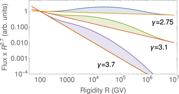
Figure 2. Bump strengths in the CR spectra with different spectral indices corresponding to the helium and boron LIS (Table 2), and γarb = 3.7 (for illustration), calculated using Equation (9) and compared to the straight background power laws. The ratios of the enhanced fluxes at R = 30 TV to the background values for the three different values of γ are 2.46, 3.06, and 6.05, respectively.
Download figure:
Standard image High-resolution imageFigure 3 shows the primary helium and carbon spectra. The DAMPE and CREAM helium spectra were normalized to the helium LIS by applying factors 1.08 and 1.05, correspondingly. Following Adriani et al. (2020) the CALET spectrum of carbon was multiplied by 1.27 to agree with AMS-02 data. Given the same spectral indices below the first break  , the shapes of helium and carbon spectra are identical.
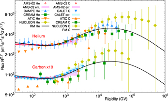
Figure 3. The calculated helium and carbon spectra are compared with available helium data from AMS-02, DAMPE, CREAM, ATIC, and NUCLEON (Panov et al. 2009; Yoon et al. 2017; Karmanov et al. 2020b; Alemanno et al. 2021; Aguilar et al. 2021) and carbon data from AMS-02, CALET (multiplied by 1.27), ATIC, CREAM, and NUCLEON (Ahn et al. 2009; Karmanov et al. 2020a; Adriani et al. 2020; Aguilar et al. 2021). The RM model calculations are using Equation (9) with parameters provided in Tables 1 and 2.
Download figure:
Standard image High-resolution imageWe are also comparing our model calculations with the measurements of the B/C ratio that is widely used to evaluate the CR residence time in the Galaxy. It is measured in a wider rigidity range and with higher precision than the individual spectra of boron and carbon. Figure 4 shows the calculated B/C ratio compared with available data. The inset shows the ratio multiplied by a factor R0.3 to emphasize the fine details in the bump range. Our model shows ≈10% deviation from predictions for the Kolmogorov turbulence ∝ R−0.33 (Kolmogorov 1941) in the bump range.
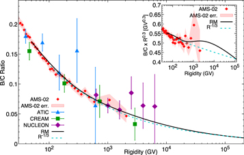
Figure 4. The calculated B/C ratio is compared with AMS-02, CREAM, ATIC, and NUCLEON data (Ahn et al. 2008; Panov et al. 2008; Grebenyuk et al. 2019b; Aguilar et al. 2021). The RM model calculations are done using Equation (9) with the parameters provided in Tables 1 and 2.
Download figure:
Standard image High-resolution image6. Background Spectra
Here we comment on the origin of the background spectra of different CR species below  . A physical explanation for the observed difference between γp
and γs
of primary elements with effective mass-to-charge ratios
. A physical explanation for the observed difference between γp
and γs
of primary elements with effective mass-to-charge ratios  ≈ 2, or higher has already been suggested (Malkov 1998; Malkov et al. 2012; Hanusch et al. 2019). They develop harder than proton spectra (the index difference γp
−γs
≈ 0.1) because SNR shocks extract them from thermal plasma most efficiently when these shocks are at their strongest. The time-integrated spectra of heavier elements then become harder than that of the protons.
≈ 2, or higher has already been suggested (Malkov 1998; Malkov et al. 2012; Hanusch et al. 2019). They develop harder than proton spectra (the index difference γp
−γs
≈ 0.1) because SNR shocks extract them from thermal plasma most efficiently when these shocks are at their strongest. The time-integrated spectra of heavier elements then become harder than that of the protons.
This bias stems from the shock-related turbulence, whose amplitude increases with the Mach number. Resonantly driven by protons, it curbs them tighter downstream than heavier nuclei, so the latter may cross the shock to gain energy. As the above differentiation mechanism depends exclusively on  , its salient consequence is that all elements with the same
  must have the same ultrarelativistic rigidity spectra (Malkov 2018). No exceptions to this rule have been reported so far (Aguilar et al. 2021).
The steep background spectrum of the secondaries is related to a decreasing residence time of CR species in the Galaxy as rigidity increases. The secondaries are already produced in fragmentations of primary CRs with a steep spectrum that is further steepened due to the rigidity-dependent residence time.
7. Discussion
There is no reason to believe that the observed bump in the CR spectrum is unique. Similar bumps might be generated in other Galactic locations where shocks are present. Whether their integral contribution competes favorably with the CR reacceleration by the ISM turbulence is too early to say. Theoretical estimates of the turbulent reacceleration (Seo & Ptuskin 1994; Ptuskin et al. 2006; Drury & Strong 2017) suggest that it supplies up to 50% of the power required to maintain the CRs against losses. However, this estimate is difficult to confirm using observations, as the reaccelerated CRs are inseparable from the background.
By contrast, a contribution of CR-reaccelerating shock is identifiable, and as we argued, is currently observed. The next step is to create an inventory of such shocks and integrate their contributions. Our results show that such shocks can temporarily modify the local CR spectrum. Studies of time-dependent CR transport show similar modifications (Porter et al. 2019). However, the significance of our result is that we do not need such a major event as a supernova explosion nearby to modify the local CR spectrum.
The local interpretation of the 10 TV bump has broader consequences in terms of our understanding of the CR spectrum. First, the B/C ratio is also affected by such modifications. Hence, the observed B/C ratio cannot be used to estimate the CR confinement time without corrections for the reacceleration effects due to the passing stars and other shocks in the local ISM. We speculate that even the well-known knee at ∼3 PV could also be interpreted as a big bump in the following fashion. The spectrum hardens below the knee due to a reacceleration by some shock, which is consistent with observations. How exactly it hardens is not clear since these observations are not nearly as accurate as the new observations in the region ≲10 TV discussed in this paper. The local shock that might be responsible for the reacceleration needs to be 2–3 orders of magnitude larger, e.g., a spiral density shock (Shu et al. 1972). According to Equation (2), weaker shocks substantially affect steep background CR spectra. The knee itself is then generated by physical processes similar to those responsible for the 10 TV bump formation addressed earlier.
Returning to the subject of this paper, let us discuss possible local CR reaccelerators. Apparently, the reacceleration power requirements are modest because the background CR spectrum is steep (∝ R−2.85). Its slight upshift (by a factor of ≈1.36) in rigidity suffices for the bump to be formed. However, its fine structure depends on the self-generated turbulence (Paper I), through which the reaccelerated CRs propagate to the observer along the magnetic field. The low-energy reaccelerated particles (R ≲ 1 TV) do not reach the observer as they are convected downstream with the ISM flow. This low-energy screening makes the distance to the object a defining parameter for the bump.
A more detailed formalism in Paper I shows that the observed bump is a factor 2.4 enhancement over the background spectrum at its maximum near 10 TV (after the spectrum is multiplied by R2.7). Even a weak shock of a size comparable with the particle Larmor orbit can provide the required upshift, operating in an SDA (shock-drift acceleration) regime. All it takes is that the shock overruns a significant portion of the particle Larmor orbit before the particle escapes the shock front along the field line. The full orbit crossing time is rg
/Ushock ≈ 30 yr for rg
∼ 3 × 1015 cm (a 10 TV proton in a 10 μG field
4
) and Ushock ≈ 30 km s−1. The flow near the shock front is likely turbulent, so the particle confinement in the field direction can be taken at the Bohm level. Particles do not diffuse beyond  from the shock during the orbit crossing.
While these numbers appear restrictive for the Epsilon Eridani bow shock, which is 8000 au ∼1017 cm, it can still cross orbits of 10 TV particles before they diffuse away along the field. The bow-shock tail may even exceed 104 au. Because the quasi-one-dimensional diffusion of particles along the field is recurrent, they will have a fair chance to interact with the shock repeatedly and climb up its flanks to the apex, thus gaining more energy via the SDA process. Stronger nondiffusive confinement of particles to a bow shock near its head is also possible by modifying the shock magnetic environment by energetic particles themselves. For example, such phenomena are observed at the Earth’s bow shock (magnetic cavities, hot flow anomalies, etc., Sibeck et al. 2021). In addition, the diamagnetically expelled field ahead of the shock may create a magnetic trap for the particles, thus extending their interaction with the shock (see the Appendix). The particle energy gain after a single Larmor-circle shock crossing can be inferred from the conservation of the particle magnetic moment:  , where p⊥ is a component of particle momentum perpendicular to the B-field. Therefore, even a factor of 2 magnetic field compression would suffice to make the bump visible.
The above constraints on the energy gain may be further relaxed in the case of a powerful stellar wind TS (e.g., Epsilon Eridani star), as the shock speed is likely to exceed the bow-shock velocity by two orders of magnitude (see the Appendix). In addition, the Cranfield–Axford effect (Axford 1972) may substantially increase the magnetic field in the surrounding area filled by the shocked stellar wind. Analytic models for the CR spectrum repower by the stellar terminal shocks are available (e.g., Webb et al. 1985), showing a relatively high, typically 40% efficiency of the wind energy conversion into the reaccelerated CRs. Observations also indicate that powerful stellar winds accelerate particles efficiently (Rangelov et al. 2019).
Shocks that are significantly larger than stellar bow shocks are almost certainly present in the solar system proximity and can remove the maximum energy restrictions. We have discussed possible origins and even tantalizing evidence for their existence in the Local Bubble (Gry & Jenkins 2014; Paper I). However, the Epsilon Eridani is particularly appealing being well aligned with the direction of the local magnetic field, yet fitting the basic model restrictions. A serious contradiction of a large-shock scenario comes from the angular distribution of the bump particles. It is much easier to reconcile the anisotropy data with a smaller shock and a narrow propagation channel pertinent to the Epsilon Eridani. We, therefore, provide in the Appendix a compound acceleration model tailored for this star in which both the bow shock and the stellar wind TS are synergistically involved in the SDA process.
We thank Samuel Ting, Andrei Kounine, and Vitaly Choutko for numerous discussions of the AMS-02 data, John Krizmanic, Kazuyoshi Kobayashi, and Shoji Torii for discussions of the CALET data, Jin Chang and Qiang Yuan for providing the DAMPE data prior to their publication and discussions, Dmitry Podorozhny, Alexander Panov, and Andrey Turundaevsky for providing the updated data of NUCLEON and ATIC, and Eun-Suk Seo for providing the CREAM data. We also acknowledge numerous discussions with Pat Diamond. M.A.M. acknowledges support from NASA ATP-program under grant No. 80NSSC17K0255 and from the National Science Foundation under grants No. NSF PHY-1748958 and AST-2109103. I.V.M. acknowledges support from NASA grant Nos. NNX17AB48G, 80NSSC22K0718, 80NSSC22K0477.
Appendix A: Compound Acceleration Model
The purpose of this appendix is to demonstrate that under a favorable but realistic B-field configuration, the interaction of particles with the TS is longer than in the standard SDA cycle and results in a larger than the  momentum gain, where r is the compression ratio. We show that the interaction of the star’s bow shock with its wind TS in the Epsilon Eridani system and its peculiar location makes it a viable candidate source of the observed 10 TV CR bump.
A.1. Motivation and Physical Context
A particle acceleration model that would combine a star’s bow shock with its wind TS is motivated by overwhelming evidence of the Local Bubble origin of a 10 TV bump, discussed in the Introduction. The potential efficiency of this model is supported by studies of colliding plasma flows in astrophysical (e.g., Bykov 2001) and laboratory (e.g., Malkov & Sotnikov 2022) settings. Here we focus on a collision region between the stellar wind and the inflowing ISM wind.
The absence of traditional CR sources, such as SNRs, in our proximity raises the bar for potential accelerator efficiency. In Paper I, we entertained the following three types of possible sources: (i) a radiative shell of an old SNR or magnetoacoustic shock formed by wave steepening, (ii) imploding shock within a monolithic Local Bubble model inferred by Gry & Jenkins (2014) from their observation analysis, and (iii) a stellar bow shock. Shocks from (i) and (ii) variety, being comparable in size with the distance to them, easily provide the required flux of reaccelerated CRs into the 10 TV range at the observer’s location. Indeed, lateral losses of CRs from the flux tube in Equation (9) are not important, given a significant size-to-distance ratio of such source. By contrast, this ratio is rather small even for a nearby stellar bow shock and the lateral spread of reaccelerated CRs might make the bump unobservable near the Sun. On a potentially positive side, the bow-shock scenario provides a unique opportunity to associate the observed CRs with familiar objects, thus increasing the persuasiveness of this scenario. Adding the serendipitously close (within 67) alignment of a nearby (ca. 3.2 pc) Epsilon Eridani star with the local magnetic field direction warrants a closer look at this object as a likely source of the CR bump.
Our interest in this object is also driven by the angular distribution of CRs in the rigidity range where the observed CR bump is located. We have discussed this aspect of the bump phenomenon in Paper I (see Section 7 and Appendix D). We have shown that if the source of the bump is located on one side of the magnetic field line in a limited range of 3–10 pc, the observed spectrum will have an anisotropy characterized by a sharp rise across the magnetic horizon, which is actually observed (Abeysekara et al. 2019). Sources located at larger distances would have produced a much smoother angular CR distribution. This is equally true for the rigidity dependence of the CR spectrum in the bump area, discussed earlier.
Estimates of the energy gained by particles after crossing a stellar bow shock (Section 7) and the propagation losses (Section 3) demonstrate that Epsilon Eridani’s bow shock can marginally account for the bump in terms of its magnitude. At the same time, additional losses, e.g., those discussed in Paper I may raise the required CR reacceleration rate at the source. We therefore consider the possibility of CR reacceleration at the stellar wind TS as a booster for particles that have already passed through the bow shock and increased their energy, Figure 5.
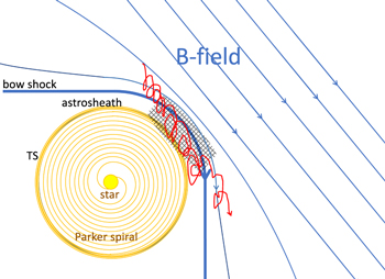
Figure 5. Stellar wind cavity showing the TS and bow shock ahead of a moving star. The hatched area covering the adjacent portions of the bow shock and TS is a magnetic trap for CRs (see text).
Download figure:
Standard image High-resolution imageA.2. Model Description and Estimates of Its Efficiency
Let us first consider plasma conditions in the region between the stellar wind TS and the bow shock that includes the astropause (that can be characterized as such using its analogy with the heliopause). This is a turbulent zone of colliding flows where thermal particles may undergo stochastic acceleration (e.g., Brunetti & Lazarian 2007; Lemoine 2021). However, their energy would not be sufficient to reach the solar system, so we focus on the reacceleration of preexisting CRs.
Particles with energies up to tenths of teraelectronvolts have Larmor radii comparable to the thickness of the shocked plasma layer between the bow shock and TS. Gyrating along this layer, as shown in Figure 5, they visit the stellar wind cavity where a motion electric field E ∼ USW B/c, accelerates them. Here USW is the velocity of the stellar wind. As their perpendicular momentum increases by a factor Δp⊥/p⊥ ∼ USW/c each time they cross and recross the TS, the pressure of CRs in this area (shown by a hatched rectangle in Figure 5) is higher than the ambient CR pressure. By the pressure balance, the field strength should be lower in this area, thus developing a magnetic cavity. We may ignore the effect of the ISM wind ram pressure of the inflowing plasma for now, as the star velocity is relatively low, ≈30 km s−1. However, cumulative effects of the magnetic flux expelled from the cavity, flow compression behind the shocks, involvement of neutrals, and general flow pattern past the astrosphere result in a magnetic barrier around the cavity. Therefore, not only do the particles inflowing from the bow-shock apex with p⊥ ≫ p∥ become trapped, but also field-aligned particles around the cavity have a good chance of being trapped adiabatically into the magnetic cavity and stay there, as they are scattered in pitch angle. The adiabatic trapping into a magnetic cavity is quite similar to that into an electrostatic potential well, as described by Gurevich (1968). We, therefore, omit the details and focus on the interaction of the trapped particles with the TS.
A.3. Dynamics of Trapped Particles
The purpose of this analysis is to demonstrate that under a favorable but realistic B-field configuration, the interaction of particles with the TS is longer than in the standard SDA cycle, and therefore, results in a momentum gain larger than  . It results from the particle orbit crossing by a shock with the compression ratio r. Under the favorable magnetic configuration we understand the one where the Parker spiral field is roughly aligned with the field between the bow shock and TS. Specifically, we assume that the B-field is out of plane on both sides of the TS surface, Figure 6. For simplicity, the curved bow shock and TS are shown as planar shocks. Upstream of it, the particle inscribes an arc in the local fluid frame. The orbit’s continuation downstream is more complex, as the motion electric field is not constant there and cannot be eliminated by the frame transformation. Indeed, the flow on the downstream side of the TS is established by its collision with the ISM flow downstream of the bow shock. The resulting flow is deflected along the TS–bow-shock direction away from the flow stagnation region. In and around this region the flow speed is much lower than USW and we may neglect the effect of the outflow, that is the effect of the motion electric field on the 10 TV particles. In this case, the particle orbit is also a part of a circle in the frame fixed by the positions of the TS and bow shock, and thereby the magnetic trap.
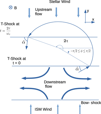
Figure 6. Mechanism of acceleration of particles entering the wind cavity from the downstream of the TS. Particles enter the upstream side of the TS from the astrosheath, propagate along an arc in the stellar wind frame, and return to the astrosheath. Positions of the TS (T-Shock) at these moments are shown with horizontal lines.
Download figure:
Standard image High-resolution imageAssuming that a particle in the magnetic trap enters the wind cavity through the TS at an angle  and returns at angle
  , as shown in Figure 6, we shall obtain the momentum gain in terms of the entry phase upstream, ϕ:
and the upstream rotation phase, 2τ, where τ is a root of the following transcendental equation:

Here v⊥ is perpendicular to the B-field component of particle velocity and USW ≪ c. The equation above can be derived by assuming that while the particle makes an arc 2τ upstream of the TS the shock itself progresses to a distance 2τ USW/ωc in the upstream frame. Note that as long as particles are in the magnetic trap, their average pitch angle remains close to π/2 and we can set v⊥ ≈ c. We represent the momentum gain as a ratio of the particle Lorentz factors after and before it visited the wind cavity
After reentering the downstream space at the angle 
the particle gyrates around its guiding center fixed in the TS frame, as we assumed above. Equations (A1)–(A3) determine an iterated map  (Figure 7). In the next cycle, the TS entrance angle
  will be different from
  in general, but after several such visits, the exit angle
  approaches the entrance angle
  . In other words, the iterations converge to a fixed point
  . This fixed point is stable, since
  at
at  .
.
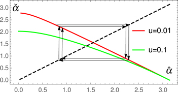
Figure 7. Iterated map  . It is constructed by a superposition of the map
  (shown with solid lines for two different stellar wind speed, u = USW/c) and the identity map (shown with a dashed line, see text). Arrows show the first two iterations of an infinite series that ultimately converges to a fixed point. The case of a faster shock with u = 0.1 is also shown for comparison with a green line.
Download figure:
Standard image High-resolution imageA.4. Results and Application to the Epsilon Eridani Star
Since the stellar wind is nonrelativistic, USW ≪ c, from Equations (A1) and (A2) we find  and ϕ ≈ π
USW/2. Under these conditions, the energy gain tends to η ≈ 1 + 2USW/c. It corresponds to the energy gain of a particle specularly reflected from the medium moving at the speed USW, as expected. The question that arises is for how long a particle can remain in the magnetic trap and keep gaining momentum Δp⊥/p⊥ = 2USW/c after each rotation.
and ϕ ≈ π
USW/2. Under these conditions, the energy gain tends to η ≈ 1 + 2USW/c. It corresponds to the energy gain of a particle specularly reflected from the medium moving at the speed USW, as expected. The question that arises is for how long a particle can remain in the magnetic trap and keep gaining momentum Δp⊥/p⊥ = 2USW/c after each rotation.
To give a simple answer to this question, we consider the energy range wherein the above acceleration mechanism operates. The upper bound is set by the particle gyroradius not to exceed the size of the magnetic trap. Using the results of Wood et al. (2002), we may assume that the size of the trap across the field is ∼103 au. As the field outside of the magnetic cavity should be enhanced according to the above considerations and the Axford–Crandfield effect (Axford 1972) to about 10 μG, particles of several tenths of teravolts can be confined to the cavity and accelerated, even though the field should be diminished inside.
Using the available data about the Epsilon Eridani star, we may also estimate the stellar wind velocity USW that determines the particle acceleration rate. The required parameters are the mass-loss rate  , which is about
  and the standoff distance of TS being RSW ∼ 103 au at its minimum on the upwind side of the moving star (Wood et al. 2002). Since these are very crude estimates, we simply assume that Epsilon Eridani is moving through the ISM, similar to that around our heliosphere, that is with the same pressure and the ISM wind having nearly the same speed. Therefore, the ram pressure at the TS is also nearly the same:
  . From the mass-loss ratio of 30, we obtain
  , where the index SW refers to Epsilon Eridani. We, therefore, obtain
  and find that the momentum gain per cycle is Δp⊥/p⊥ = 2USW/c ∼ 10−2. We thus conclude that particles trapped in the magnetic cavity for ~100 gyro periods gain additional energy comparable with that they gained by crossing the stellar bow shock.
Footnotes
- 3
The mostly secondary species are those, which are rare in CR sources, but abundant in CRs. They are produced primarily in fragmentations of heavier species over their lifetime in the Galaxy.
- 4
The direct measurements of Voyager 1, 2 give 7–8 μG just outside of the heliosphere (Burlaga et al. 2019).