Abstract
We present analysis of one of the most extreme quasar outflows found to date in our survey of extremely high-velocity outflows (EHVOs). J164653.72+243942.2 (zem ∼ 3.04) shows variable C ivλλ1548,1551 absorption at speeds larger than 0.1c, accompanied by Si iv, N v, and Lyα, and disappearing absorption at lower speeds. We perform absorption measurements using the apparent optical depth method and SimBAL. We find the absorption to be very broad (Δv ∼ 35,100 km s−1 in the first epoch and 13,000 km s−1 in the second one) and fast (vmax ∼ –50,200 km s−1 and −49,000 km s−1, respectively). We measure large column densities ( 21.6 (cm−2)) and are able to place distance estimates for the EHVO (5 ≲ R ≲ 28 pc) and the lower-velocity outflow (7 ≲ R ≲ 540 pc). We estimate a mass outflow rate for the EHVO to be
  and a kinetic luminosity of
  in both epochs. The lower-velocity component has a mass outflow rate
  and a kinetic luminosity of
  . We find that J164653.72+243942.2 is not an outlier among EHVO quasars in regard to its physical properties. While its column density is lower than typical BAL values, its higher outflow velocities drive most of the mass outflow rate and kinetic luminosity. These results emphasize the crucial role of EHVOs in powering quasar feedback, and failing to account for these outflows likely leads to underestimating the feedback impact on galaxies.
Original content from this work may be used under the terms of the Creative Commons Attribution 4.0 licence. Any further distribution of this work must maintain attribution to the author(s) and the title of the work, journal citation and DOI.
1. Introduction
Active galactic nuclei (AGN) are found at the centers of most massive galaxies. Among them, quasars show the largest luminosities, allowing us to study them at large redshifts and providing information about galactic evolution within our Universe. Understanding the connection between the inner region and the surrounding host galaxy has proven crucial, as evidence of a coevolution scenario through feedback processes has been mounting in the form of the tight correlation between the masses of supermassive black holes (SMBHs) and the stellar spheroids of their host galaxies (Mbulge; e.g., K. Gebhardt et al. 2000; D. Merritt & L. Ferrarese 2001; S. Tremaine et al. 2002), and the need for regulating star formation in the host galaxies (e.g., J. Silk & M. J. Rees 1998; T. Di Matteo et al. 2005; V. Springel et al. 2005; P. F. Hopkins et al. 2006).
One promising way to connect the two regions is through outflows: gaseous material outflowing from the central engine into the galactic host. In fact, simulations have shown that cosmological feedback from AGN outflows and jets is a needed regulating mechanism (e.g., J. Silk & M. J. Rees 1998; T. Di Matteo et al. 2005; V. Springel et al. 2005; P. F. Hopkins et al. 2006; X. Ding et al. 2020). Moreover, outflows need to be understood on their own merits: They are fundamental constituents of AGN, and they provide first-hand information about the physical and chemical properties of the AGN environment and the SMBHs. They are detected in a substantial fraction of AGN through absorption-line signatures (e.g., broad, blueshifted resonance lines in the UV and X-ray bands) as the gas intercepts some of the light from the central continuum source and broad emission-line region (e.g., D. M. Crenshaw et al. 1999; T. A. Reichard et al. 2003; J. R. Trump et al. 2006; D. Nestor et al. 2008; A. L. Rankine et al. 2020; H. Choi et al. 2022b, and references therein). Outflows could be ubiquitous, though, if the absorbing gas subtends a small solid angle around the background source.
For simplicity, large UV/optical surveys of quasar outflows have focused on searching for broad C iv absorption that would indicate gas outflowing at speeds less than 0.1c; typically referred to as broad absorption line quasars (BALQSOs). This arbitrary velocity limit was defined to avoid complications due to misidentification with Si iv or other ionic transitions blueward of the Si iv emission line. However, gas outflowing at extremely high speeds might be the most disruptive if it reaches the host galaxy environment, as it may provide large kinetic power. Outflows with speeds v ∼ 0.2c, if the gas is located at similar distances and has similar physical properties, carry approximately 1–2.5 orders of magnitude larger kinetic power than gas outflowing at what is defined as “high” velocities (v ∼ 5000–10,000 km s−1) because kinetic power is proportional to v3. These outflows, called extremely high-velocity outflows (EHVOs; P. Rodríguez Hidalgo et al. 2011), might also pose the biggest challenges to theoretical models that try to explain how these outflows are launched and driven (F. Hamann et al. 2002; B. M. Sabra et al. 2003). Radiation pressure models (N. Arav et al. 1994; N. Murray et al. 1995; D. Proga et al. 2000; J. P. Ostriker et al. 2010, please see an excellent review in D. M. Crenshaw et al. 2003) take advantage of the powerful central source to accelerate line-driven winds and have proven successful in explaining different aspects of these winds such as the relation between the AGN luminosity and the terminal velocity of the outflow (A. Laor & W. N. Brandt 2002) and “line locking” (D. A. Turnshek 1988; R. Srianand et al. 2002; F. Hamann et al. 2011). The presence of dust mixed with the BAL gas can further boost the acceleration by radiation pressure due to the addition of scattering on dust opacity and generate outflows with velocities up to ∼1−2 × 10⁴ km s−1 (W. Ishibashi et al. 2024). However, simulations and theoretical models have faced challenges recreating the presence of detached BAL profiles with central velocities as large as 0.2c or greater (e.g., D. Proga et al. 2012; J. H. Matthews et al. 2020). Alternatively, models have also invoked magnetic forces to launch, drive, and constrain the flow (M. de Kool & M. C. Begelman 1995; D. Proga & T. R. Kallman 2004; J. E. Everett 2005), and higher terminal velocities are expected in magnetic driving due to stronger centrifugal forces (D. Proga 2007). EHVOs must be studied if we want to understand both their central inner regions and their potential effects on the galactic environment.8
Due to the arbitrary velocity limit set in the previous systematic searches, until recently, UV/optical EHVOs had only been detected in a handful of individual quasars (B. T. Jannuzi et al. 1996; F. Hamann et al. 1997a; P. Rodríguez Hidalgo et al. 2011; J. A. Rogerson et al. 2016). Our group discovered 40 new cases (P. Rodríguez Hidalgo et al. 2020; hereafter Paper I), and, more recently, an additional 98 cases (P. Rodríguez Hidalgo 2025, in preparation), by carrying systematic searches over 6760 quasars from the Sloan Digital Sky Survey (SDSS) Data Release 9 (DR9Q; I. Pâris et al. 2012) and over 18,165 quasars from the SDSS Data Release 16 (DR16Q; B. W. Lyke et al. 2020) quasar catalogs, respectively. This has resulted in the first database of EHVOs and multiplied by 30 the number of known EHVO quasars.
In our DR9Q survey (Paper I), we found a very interesting case in the spectra of J164653.72+243942.2 (hereafter J1646). J1646 shows the widest EHVO C iv absorption trough of the 40 cases found in our DR9Q survey (Δv ∼ 12,500 km s−1, measured at 90% normalized flux). J1646 (z = 3.040 ± 0.002; P. C. Hewett & V. Wild 2010) was discovered earlier in the fifth data release (DR5) of SDSS, where it was classified as a BALQSO based on C iv absorption measured at lower speeds (R. R. Gibson et al. 2009a); this absorption disappears in the DR9 observation while the EHVO remains. J1646 is a luminous radio-quiet quasar. More information on the archival spectra and quasar properties is provided in Section 2.
In this paper, we analyze the absorption in the SDSS spectra of J1646 in detail using two different methods. First, we normalize the spectrum (Section 3.1.1) and measure the absorption by the apparent optical depth (AOD) method (Section 3.3.1). This provides a conservative lower limit of the absorption measurements and the total column density and establishes a comparative baseline with other similar studies. Second, we utilize a state-of-the-art, novel spectral synthesis code, called SimBAL, that uses forward modeling to fit spectra of BALQSOs (K. M. Leighly et al. 2018), including the continuum, the emission lines (Section 3.1.2), as well as the absorption (Section 3.3.2). This code is particularly well suited to fit BALQSO spectra where the absorption is too blended to be analyzed easily by other methods. As explained in K. M. Leighly et al. (2018), SimBAL uses grids of ionic column densities generated by the photoionization code Cloudy (G. J. Ferland et al. 2017) to forward model BALQSO spectra and a Bayesian model calibration method to obtain the best-fitting values and their uncertainties. SimBAL uses forward modeling techniques, and a sophisticated mathematical implementation of partial covering allows accurate modeling of complex absorption features observed in BALQSO spectra (K. M. Leighly et al. 2019b). It has been used successfully in K. M. Leighly et al. (2018, 2019b), H. Choi et al. (2020, 2022b), and M. Bischetti et al. (2024), where a SimBAL analysis provided robust constraints on the physical properties of LoBAL outflow in a z ∼ 6.6 quasar. Also, K. S. Green et al. (2023) used SimBAL to derive physical interpretations of BAL variability seen in multi-epoch Hubble Space Telescope (HST) observations of the narrow-line Seyfert 1 WPVS 007. Finally, in Section 4, we discuss the implications of these results and comparisons to studies of absorption at lower velocities or other wavelength ranges.
2. Data and Quasar Properties
2.1. Archival Spectra
The data used in this paper are archival spectra from SDSS (D. G. York et al. 2000). We discovered the special characteristics of the absorption in the spectrum of J1646 during a survey of EHVOs (Paper I) carried out over the SDSS DR9Q quasar catalog (I. Pâris et al. 2012), which was derived from the Baryon Oscillation Spectroscopic Survey (BOSS; K. S. Dawson et al. 2013) of SDSS-III (D. J. Eisenstein et al. 2011). Another previous spectrum taken ∼1.70 yr earlier in the quasar rest frame was already available from SDSS DR5 (D. P. Schneider et al. 2007). Table 1 includes observation dates, wavelength coverage, and signal-to-noise ratio (S/N) of the spectra used in this paper. The resolution of both spectra is 1500 at 3800 Å (2.5 Å).
Table 1. Date and Spectral Characteristics of the SDSS DR5 and BOSS DR9 Data Used in This Work
| DR | MJD | Date | Spectral Coverage | S/N |
|---|---|---|---|---|
| (YYYY-MM-DD) | (Å) | |||
| DR5 | 53167 | 2004-06-11 | 3800–9200 | 20.9a |
| DR9 | 55685 | 2011-05-04 | 3600–10500 | 20.0746b |
Notes.
aS/N = 1700 in R. R. Gibson et al. (2009b). bS/N = 1700 in I. Pâris et al. (2012).Download table as: ASCIITypeset image
Figure 1 shows both spectra (DR5 and DR9) overplotted. For easy visualization, we have smoothed both spectra with an 11-pixel boxcar. The spectra were wavelength calibrated and sky subtracted by the SDSS pipeline. Both spectra have been dereddened for Galactic extinction using the extinction curve of J. A. Cardelli et al. (1989), assuming R = 3.1 and an E(B − V) value of 0.0495 from D. J. Schlegel et al. (1998). The continuum is clearly higher in the early observation (DR5),9 but the maximum absorption depth appears at a similar flux level in both observations. This is not uncommon, as we detail in P. Rodríguez Hidalgo et al. (2025, in preparation). The rest-frame wavelengths here and elsewhere in this paper are defined relative to the redshift zem = 3.040 from P. C. Hewett & V. Wild (2010).
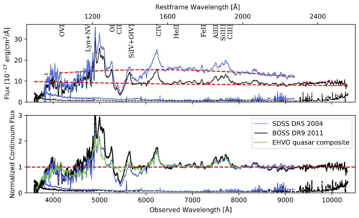
Figure 1. Spectra of J1646 in SDSS DR5 (blue) and BOSS DR9 (black), observed (top) and continuum normalized (bottom), with their corresponding error spectra at the bottom of each figure. All spectra have been smoothed with an 11-pixel boxcar for easy visualization. Absorption is clearly visible in both spectra at an observed frame of ∼5400 Å, with additional absorption present in the SDSS DR5 spectrum around ∼5900 Å. Top panel: the rest-frame wavelength is shown at the top of the figure, and typical emission lines are indicated on top of the SDSS spectrum. The red dashed lines correspond to our continuum normalizations of the spectra in Section 3.1.1. Bottom panel: we also include a composite EHVO spectrum derived from our Paper I (green). In this case, the dashed red line is included to indicate the normalized continuum level and help guide the eye.
Download figure:
Standard image High-resolution image2.2. Quasar Properties
J1646 (z = 3.040 ± 0.002; P. C. Hewett & V. Wild 2010) is a luminous quasar: SDSS provided a magnitude of g = 18.80 (MJD = 52760) and Y. Shen et al. (2011) calculated an absolute i-band magnitude, K-corrected to z = 2 (Mi[z = 2]) of −28.9 (MJD = 53167).
A. L. Rankine et al. (2020) provided improved values of physical properties of DR14 quasars by producing spectrum reconstructions covering the rest frame 1260−3000 Å of 144,000 quasars. These spectrum reconstructions were generated by mean field independent component analysis using the information across the entire spectrum to inform the reconstruction. A. L. Rankine et al. (2020) provided values for J1646 of bolometric luminosity ( 47.25 (erg s−1)), black hole mass (
 /M⊙ = 9.5), and Eddington ratio (
 /LEdd = −0.4) using the MJD = 55685 observation. Black hole masses were calculated using the C iv emission line but accounting for the excess nonvirial blue emission for quasars with large C iv blueshifts (L. Coatman et al. 2017). Neglecting to account for this correction results in overestimated black hole masses and, therefore, also miscalculated Eddington ratios. In fact, for J1646, the C iv blueshift is significant (∼2470 km s−1). This seems to be typical in EHVO quasars, which show larger blueshifts than BALQSOs and non-BALQSOs in general (P. Rodríguez Hidalgo & A. L. Rankine 2022). The black hole mass measurements have an uncertainty of ±0.5 dex, accounting for both systematic effects and measurement errors; see Section 6.3 in A. L. Rankine et al. (2020) for more information. These values should be taken as a rough estimate due to the variability in this object; as mentioned, they were calculated using the second observation (DR9; MJD = 55685). Given that the continuum shows large variability (see Figure 1) and the flux was larger during the first observation (DR5), it is likely that the bolometric luminosity of the quasar was also larger in the first observation.
J1646 is a radio-quiet quasar as it has no identified match to a Faint Images of the Radio Sky at Twenty centimeter source included in I. Pâris et al. (2012).
3. Analysis and Results
3.1. Normalization of the Quasar Spectra
To perform measurements of the absorption, we first normalized both spectra. Quasars tend to show negative-sloped spectra in the UV/optical region, and composite quasar spectra are well approximated by a power law in this region, even in the far-UV (e.g., D. E. Vanden Berk et al. 2001; R. C. Telfer et al. 2002; E. M. Tilton et al. 2016). In Paper I, we performed a systematic normalization of the 6760 quasar spectra in the sample, focusing on the wavelength region between the Lyα+N v and C iv emission lines, in order to search for and measure EHVO absorption in that wavelength range. For the work in this paper, we have refined the normalization of the J1646 spectra to include the Lyα forest region, and a more tailored fitting of the region redward of the C iv emission line.
Throughout this paper, we show two different procedures, performed independently, to characterize the absorption in the J1646 spectra: (1) the AOD method, for which only the underlying continuum is fitted; this methodology provides a solid lower limit for the outflow measurements, and (2) a best estimate one, using SimBAL (described in Section 1), where the continuum, emission, and absorption are fitted simultaneously. In the subsequent sections, we describe how we used both methods to analyze the continuum and emission lines in the spectra (Sections 3.1.1 and 3.1.2), identify (Section 3.2), and measure the absorption (Sections 3.3.1 and 3.3.2).
3.1.1. AOD Approach: Continuum-fitting and Emission-line Analysis
As can be seen in Figure 1, the continua between both epochs differ not only in flux level but also in slope. Therefore, we followed different approaches to fit the continuum for each spectrum.
For the BOSS DR9 2011 spectrum, we used a simple power law (similar to what is shown in Figure 6 of D. E. Vanden Berk et al. 2001) anchored at four points in the quasar spectra. All anchor points were selected away from emission and absorption features. The power law seems to match the continuum correctly throughout the spectrum.
For the SDSS DR5 2004 spectrum, a single power law did not produce an adequate fit, as the continuum seems to curve down at shorter wavelengths. This is not rare: The composite spectrum by R. C. Telfer et al. (2002), which was made from a sample of 332 HST Faint Object Spectrograph quasar spectra, required a broken power law to fit the continuum blueward of the Lyα+N v emission line. Then, a simple power law would have overestimated the absorption in this region.
The normalization of the Lyα forest is complicated due to (1) the combination of a myriad of hydrogen absorption lines and the presence of emission lines such as O vi λλ1032,1038, and (2) in our case, being a narrow wavelength region located at the edge of the SDSS/BOSS spectrum where the sensitivity and S/N are reduced. Thus, for both spectra, we tried to extrapolate a reasonable fit from the wavelength region redward of the Lyα+N v emission line into the Lyα forest without selecting any point to anchor the fitting in this complex region. For the DR9 spectrum, the simple power law produces a reasonable continuum in this region. For the DR5 spectrum, a second-order polynomial function mimics the broken power law and allows us to extrapolate the fitting blueward of the Lyα+N v emission line into the Lyα forest. All of the anchoring points were selected redward of the C iv emission line since the region between the Lyα+N v and C iv emission lines (∼1200–1600 Å in the rest frame) contains an entangled combination of emission lines and broad absorption.
Figure 1 also shows the normalized spectra that were obtained by dividing the original spectra by each continuum fitting. While both normalizations were carried out independently and through different methods, as explained above, many of the emission lines overlap, including the O vi emission line. We include as well a composite (green) derived from our survey of EHVO quasars in Paper I. This weighted-mean composite is created by combining the 16 cases with 2.5 < zem < 3.25 (approximately the middle third of our DR9 sample), which we resampled by interpolating to a common wavelength grid prior to averaging. We selected these quasars for the composite because our survey of EHVO DR9 quasars found a large range of redshifts, and the Lyα emission line shows very different contaminations with Lyα forest lines depending on quasar redshift. We do not mask the absorption, and thus, it appears averaged in the composite. This approach is conservative, and we might be underestimating the continuum levels of both spectra, especially the SDSS DR5 spectrum, if additional absorption is present. However, it is very unlikely that we have overestimated the continuum levels: In R. C. Telfer et al. (2002), the elbow of the broken power law occurs at the Lyα+N v emission line, not redward of it. Absorption measurements using this method will thus be lower limits.
While we do not fit the emission lines within this approach, we took advantage of having two epochs of spectra and noticed that the emission lines are very similar between epochs. Figure 1 also shows the emission lines in the 6000–8000 Å region (C iv, He ii, Fe ii, Al iii, C iii], labeled at the top of the figure) resemble each other quite well and they seem to differ only by a scaling factor.
Even in the region where absorption is clearly present, emission lines appear to retain their shape and to be displaced downwards. In the DR9 BOSS spectrum, C ii could be part of the absorption profile. In the DR5 SDSS spectrum, O i, C ii, and Si iv+O iv] emission lines may be embedded within the absorption profile; this is very clear in the case of the Si iv+O iv] emission line, which appears to be surrounded by absorption (see Figure 1, ∼1400 Å in the rest frame, ∼5700 Å in observed wavelength). Without access to a different epoch, it could have been interpreted as if the emission line had been completely absorbed.
Using the similarities between emission lines in the two epochs, which correspond to a wide range of physical conditions, we took a comparative approach. We assumed that the absorption in the DR9 spectrum is restricted to absorbing the continuum and that the emission lines surrounding absorption features (such as O i and Si iv+O iv]) are not affected by it. Figure 2 shows the method we used. We created a template of emission lines, which we call the scaled DR9 template, by interpolating the BOSS spectrum to the wavelength grid of the SDSS spectrum and using the region between rest frame 1500 and 1950 Å (between the C iv and Al iii+C iii] emission lines) to determine the scaling factor (Figure 2, top). Using the normalized spectra, the scaling factor was the value that minimized the median of the values for ((BOSS DR9 1) × (scaling value) + 1) – SDSS DR5, in this region. Figure 2 (top) shows the scaled BOSS DR9 spectrum (blue) overplotted together with the SDSS DR5 spectrum. Figure 2 (middle) shows how close the emission lines of the scaled DR9 match the DR5 spectra. Finally, we divided the SDSS DR5 spectrum by the scaled BOSS DR9 spectrum.
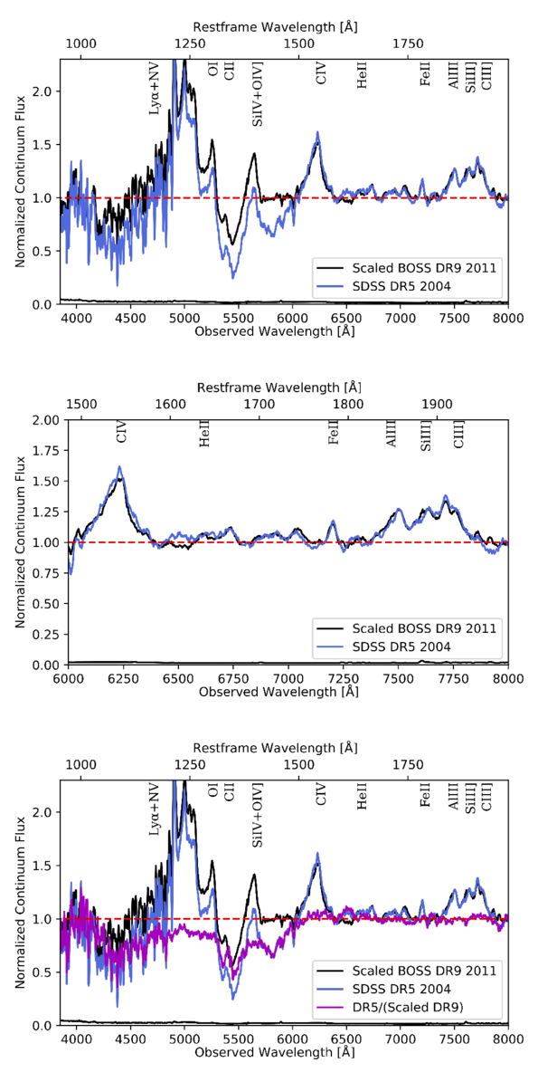
Figure 2. Top and middle panels: scaled BOSS DR9 spectrum (black) overplotted over the SDSS DR5 spectrum (blue), showing the whole spectra (top) and only the region used to find the scaling factor (middle). Bottom panel: original DR5 spectrum (blue) and masked and scaled BOSS DR9 spectrum (black) overplotted together with the divided spectrum of the two (magenta). All spectra have been smoothed by an 11-pixel boxcar as well. Error spectra are shown below each spectrum.
Download figure:
Standard image High-resolution imageFigure 2 (bottom) shows the result of this process. The absorption in magenta represents the excess absorption in the DR5 spectrum relative to the absorption in the scaled version of DR9; in other words, it is partly the absorption that disappears between epochs. It shows that there is continuous absorption starting at ∼1480 Å up to ∼1050 Å, together with the previously distinct EHVO. The nature of the absorption is investigated in the following sections.
To ensure this very wide absorption trough was not some sort of glitch in the SDSS DR5 spectra of this object, we inspected the individual spectral exposures from the SDSS red-arm and blue-arm spectrographs. Each of the three individual exposures from each spectrograph is consistent with the others within the noise. In the region in observed wavelengths from 5825 to 6150 Å where the spectra from the two arms overlap, the average blue-arm spectrum exhibits a ≃15% lower flux level than the average red-arm spectrum, at a significance of 3.4σ assuming Gaussian statistical errors only. However, we do not believe this is strong evidence against the reality of the apparent very wide absorption trough in the DR5 spectrum. First, we do not see any blue-arm flux offsets on the two neighboring spectra on the plate. Second, multiplying the normalized DR5 spectrum by a factor of 1.15 before comparing it to the scaled DR9 spectrum does not eliminate the putative absorption trough, particularly at wavelengths just longward of Si iv. Third, the apparent very wide absorption trough absorbs an approximately fixed fraction of the normalized quasar continuum, but any plausible error in flux scaling will result in a difference spectrum feature that is a fraction of the observed spectrum, not just the continuum. Furthermore, the very wide absorption trough does not span the full wavelength range of the spectrum from the blue-arm spectrograph. Although a negative offset to the blue-arm spectrum, which happened to be constant in Fλ could match the difference spectrum given the relatively flat-in-Fλ spectrum of the quasar, such an offset would spoil the match between the normalized DR5 and DR9 spectra at the shortest wavelengths common to both spectra.
Absorption measurements in Section 3.3.1 are performed over the normalized DR5 and DR9 spectra. The findings in this section show that we are likely underestimating the amount of absorption, but it sets a firm, conservative, lower limit for it, which is our overall goal with this method.
3.1.2. Best Estimate: Continuum + Emission-line Fitting Using SimBAL
SimBAL, when it was first developed, was used to model the absorption lines alone (see K. M. Leighly et al. 2018). Instead, in this paper, as in H. Choi et al. (2020, 2022b), we modeled both the pseudo-continuum (continuum + emission features) and absorption lines simultaneously. H. Choi et al. (2022b) introduced the use of spectral principal component analysis (SPCA) eigenvectors for the emission-line modeling for rest-UV spectra within SimBAL, which we also included in this work. SPCA pseudo-continuum modeling can reproduce realistic emission-line features for a given wavelength range with fewer model parameters than individual line-fitting procedures, which require multiple parameters per emission line in the model. While SimBAL carries out the fitting of the pseudo-continuum and the absorption simultaneously, to compare with our AOD method, we describe the former in this section and the latter in Section 3.3.2.
We used a power-law model for the continuum emission for the BOSS spectrum and a broken power-law model for the SDSS spectrum to model the observed spectral shape. The slope break point for the broken power-law model was constrained to λ ∼ 1690 Å from the SimBAL fit. To fit the emission lines, we used three sets of eigenvectors because we currently do not have a single set that spans the whole SDSS/BOSS spectral region. We used one set for emission lines between 1030 and 1290 Å and another for emission lines between 1290 and 1700 Å. The first set was constructed by us using the sample of 78 z ∼ 3 quasars discussed in I. Pâris et al. (2011) and the second set was made from a sample of ∼100 quasars that show a strong blueshift in C iv emission lines, similar to what we observe in J1646 (R. Hazlett et al. 2019). Redward of 1700 Å, we used the eigenvectors described and used in H. Choi et al. (2022b), which were built from a set of 2626 SDSS non-BAL quasars. Each set of SPCA eigenvectors has six parameters: four coefficient parameters that yield the shape and the line ratios of the emission lines, and two additional parameters, the convolutional width parameter and the amplitude parameter, that control the overall strengths and the widths of the emission lines. The width parameter is not required for the standard eigenvector reconstruction. Nevertheless, we included the parameter in our model to provide it with an additional method to reproduce a broad range of emission-line widths observed in quasar spectra.
Figure 3 shows the pseudo-continuum models extracted from the best-fitting SimBAL models for SDSS DR5 and BOSS DR9. We compared our model with a composite template to examine whether our emission-line model from spectral PCA eigenvectors has produced reasonable emission-line ratios and shapes that are comparable to those observed in real data. M. J. Temple et al. (2021) provide two emission-line templates (“high-blueshift” and “high-equivalent width (EW)”) from their quasar spectral energy distribution (SED) model. We chose the “high-blueshift” template, which showed a good match with the data and our pseudo-continuum models around C iv and C iii] emission-line regions with similar line flux ratios between major emission lines (e.g., Lyα, Si iv, C iv). The “high-EW” template was disfavored as it showed a high C iv/Si iv flux ratio that we do not see in our target (see Figure 4 in M. J. Temple et al. 2021). Furthermore, since EHVOs exhibit larger C iv blueshifts in emission (P. Rodríguez Hidalgo & A. L. Rankine 2022), the high-blueshift template from M. J. Temple et al. (2021) is the most suitable for our target among the available composites (e.g., P. J. Francis et al. 1991; D. E. Vanden Berk et al. 2001). We performed an additional continuum emission subtraction between ∼1440 and ∼2000 Å because the original template showed unusually strong Fe ii emission features throughout that bandpass, and we suspected that it was contamination from inaccurate continuum subtraction. The modified emission-line template was then scaled to match the strengths of the emission lines that are not affected by BAL, such as C iv and the emission lines around C iii], and we added the scaled template to our continuum models.
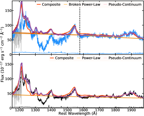
Figure 3. The pseudo-continuum model components extracted from the best-fitting SimBAL models for SDSS DR5 (top) and BOSS DR9 (bottom). Our emission-line models generated from the SPCA eigenvectors show realistic rest-UV quasar emission lines with line ratios and strengths comparable to what are found in a composite spectrum. The gray points at λ ≲ 1216 Å show the data points affected by the Lyα forest features identified by our iterative method, and they were ignored for SimBAL fitting (see Appendix A for details). The emission composite from M. J. Temple et al. (2021) is plotted in red. The vertical line in the top panel shows the location of the slope break point (λ ∼ 1690 Å) for the broken power-law model used in SDSS DR5.
Download figure:
Standard image High-resolution imageWe found that our SPCA reconstructed pseudo-continuum models match very closely with the ones made with the emission-line template. Although our object (and the models) show slightly stronger low-ionization emission lines (e.g., Si ii), major emission lines show a good match. We note that the template shows a slightly higher C iv blueshift than what is observed in our pseudo-continuum models and the data. This verifies that our SPCA reconstruction method indeed produces realistic emission-line models and also shows that J1646 has emission-line properties similar to those of quasars with highly blueshifted emission lines. For the SimBAL analysis, we employ the SPCA reconstruction method to model the pseudo-continuum. The template was used solely for comparative purposes in Figure 3.
In EHVO quasars, Si iv absorption lines are often located on top of Lyα + N v emission lines, making it difficult to estimate the true strengths of the emission complex and the amounts of Si iv opacity from the BALs. H. Choi et al. (2022b) found that in some BAL quasars, the emission lines were not absorbed by the BAL. The same phenomenon was also observed in WPVS 007 (K. S. Green et al. 2023). We modeled J1646 with and without emission-line absorption and found that a spectral model with no emission-line absorption produced a more self-consistent fit. The models with emission-line absorption predicted strong Lyα + N v emission features that are not found in EHVO quasars (see composite described above). This was because the models predicted a moderate amount of Si iv opacity near the Lyα + N v region, and in order to match the flux levels observed in that region, the models produced strong emission lines to compensate for the absorption from Si iv BAL. In contrast, the models with no emission-line absorption from the BAL produced pseudo-continuum models that resemble typical emission features seen in EHVO quasars. While this modification to the models resulted in much weaker Lyα + N v emission lines in the pseudo-continuum models than the initial model we tried, the overall BAL physical properties did not show significant differences. We note again that the continuum and line emission fitting was done simultaneously with the BAL absorption modeling.
We did not find evidence for significant emission-line variability between SDSS and BOSS (see Figure 1). Therefore, we simultaneously fit both the SDSS and the BOSS spectra, constraining the values of eigenvector coefficient parameters and the width parameters of the emission lines to be the same for both SDSS and BOSS spectra models. The continuum model parameters and the emission-line amplitude parameters were allowed to vary between the models for SDSS and BOSS, such that the EWs of the emission lines were allowed to be different for the two models while keeping the shapes of the line profiles identical.
3.2. Identification and Nature of the Absorption
Figures 1 and 3 show absorption present below the continuum at rest-frame wavelengths of ∼1360 Å in both DR9 and DR5 spectra. The absorption present in the BOSS DR9 2011 spectrum was classified as an EHVO C iv in Paper I.
In the DR5 SDSS 2004 spectrum, an absorption feature at ∼1440 Å is also clearly present. Due to the wavelength range, the most likely interpretation is as C iv outflowing at shorter velocities. Thus, this quasar would be a C iv BALQSO in the typical definition (R. J. Weymann et al. 1991) in DR5, and so it was classified (R. R. Gibson et al. 2009a).10 This trough disappears within 1.7 yr in the quasar rest frame, as it does not seem to be present in the DR9 spectrum.
3.2.1. AOD Method: Visual Identification of Other Ionic Transitions
Figure 4 includes the normalized spectra, where just the continuum has been normalized, for SDSS DR5 (left) and BOSS DR9 (right), where we have labeled the potential location of other ionic transitions. The limits of each colored region are set by the C iv absorption detection below 90% of the flux level in the normalized spectrum (red; see Section 3.3), assuming that the other ions are found at the same velocities. Due to the large absorption widths, no doublets are present to help confirm the nature of any of the absorption troughs, but C iv HiBALs are typically accompanied by N v, Si iv, Lyα, and/or O vi in the same outflow (in Figure 4, green, orange-, purple-, and blue-shaded regions, respectively), so we searched for these and other transitions at the expected wavelengths assuming they would be at similar velocities.
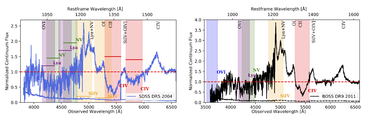
Figure 4. Spectra of J1646 in SDSS DR5 (left) and BOSS DR9 (right), including the location of potential ions with different colors. EHVO C iv absorption is indicated by a red-shaded region; the upper and lower-velocity limits are determined by the wavelengths where the absorption crosses the 90% level of the normalized flux. The DR5 spectrum also includes C iv absorption at lower velocities. The blue-, purple-, green-, and orange-shaded regions have the same lower and upper velocities as the red region but shifted to the corresponding O vi, Lyα, N v, and Si iv wavelengths, respectively; v and v
and v are included in Table 2. Although the Lyα forest is a complex region and lies at the edge of the spectrum, the width of the absorption and the changes between the two spectra suggest that EHVO absorption is present in both cases. O vi absorption cannot be confirmed in either spectrum because it lies at the spectral edge in DR9 and is not covered in DR5. Some emission lines present in the spectrum are labeled at the top of each figure. For clarity, in the case of the DR5 spectrum (left), we also include colored horizontal lines to mark the limits of each shaded region.
Download figure:
Standard image High-resolution imageFigure 5 shows the absorption profiles of these ions in velocity space. The left four panels show the absorption in the DR5 spectrum, and the right four in the DR9 spectrum. The top panels show the C iv absorption (red shading) with the overplotted Si iv profile (orange line) at the same outflow speed and the Si iv absorption (orange shading) with the overplotted C iv (red line). The bottom panels show the potential absorption of N v (green shading) and Lyα (purple shading), all with the C iv profile overplotted (red line). In the case of doublets, the velocity scale corresponds to the short wavelength components of the doublets relative to the emission redshift. The shaded regions are defined based on the C iv absorption and transported to the potential location of the other ions.
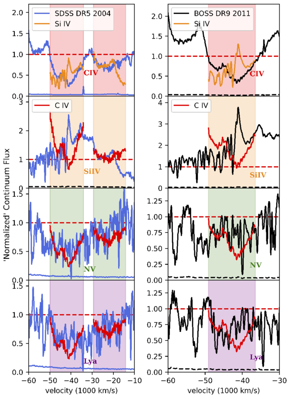
Figure 5. Normalized spectra (DR5 left, in blue; DR9 right, in black) shown in velocity space at the location of C iv (red bars, top panel in each group), and the potential detections of Si iv (orange bars, second panel), N v (green bars, third panel) and Lyα (purple bars, bottom panel). The shaded regions are defined based on the C iv absorption and transported to the potential location of the other ions. The superimposed red and orange solid lines represent the C iv and Si iv absorption profiles, respectively. The detection of EHVO Si iv lies on top of the Lyα+N v emission, but the similarity between the profiles, especially at the lower EHVO velocities in both SDSS and BOSS spectra, suggests that some Si iv absorption is present. Lyα and N v absorption overlap in spectral wavelengths and appear to be both present, but Lyα seems to be stronger, especially at the higher-velocity tail of the EHVO absorption in both epochs.
Download figure:
Standard image High-resolution imageIn Figure 4, it is difficult to assess whether the absorption at the wavelengths ∼1100 Å is due to N v or Lyα, or a combination of them, as they overlap at these absorption widths. Figure 5 (bottom left plots) shows that in the DR5 spectrum, both ionic transitions are likely to show some EHVO absorption. In both SDSS and BOSS, the profiles of Lyα and C iv follow the same shape (with the exception of Lyα forest lines) at the highest speeds of the EHVO absorber (between ∼−50,000 and ∼−43,000 km s−1), and N v absorption is also likely present at ∼40,000 km s−1 in SDSS. The absorption at a lower velocity (∼20,000 km s−1) does not present a good match between C iv and either of these two species, but the absorption is also weaker overall. In the DR9 spectrum (see Figure 5, bottom-right plots), EHVO Lyα is likely to be stronger than N v but weaker than C iv, and only the higher-velocity part of the EHVO profile appears to show potential absorption of these two species (between ∼−49,000 km s−1 and ∼−47,000 km s−1). In summary, the bottom plots in Figure 5 suggest that both Lyα and N v might be present, that their absorption profiles differ from that of C iv in that they have relatively more absorption at the highest velocities, and that Lyα absorption might be stronger than N v, especially at the higher-velocity tail of the EHVO absorption.
Based on our previous studies, we find it surprising that Lyα absorption is stronger than N v. In P. Rodríguez Hidalgo et al. (2011), we presented the analysis of other accompanying ions in the spectrum of an EHVO quasar, where N v and O vi appeared to be present, but Lyα, if present, was not strong and blended with Lyα forest lines. Other EHVO quasars in Paper I also seemed to show strong N v absorption, while Lyα absorption was much rarer than N v. Analysis of the composite shown in Figure 1 (bottom) shows how the average absorption in this region (∼1100 Å in the rest frame) favors the interpretation of N v and that the N v absorption is, on average, stronger than C iv absorption. An alternative interpretation could be that the C iv absorption is broader as it appears currently framed by two emission lines, O i and Si iv+O vi], that could be suffering some additional absorption we have not accounted for, as we discussed in Section 3.1.1. If this is the case in J1646, it might indicate either that the N v absorption is wider than the C iv absorption or that the C iv absorption is wider as well and partly present on top of the Lyα+N v+Si ii emission-line complex. Indeed, comparisons between the DR5 and DR9 spectra show that emission lines around the EHVO C iv absorption appear to be absorbed in the DR5 (Figure 1), while emission lines such as C iv and Al iii + C iii] are almost overlapping between the two spectra. Using the scaled DR9 template, the SDSS DR5 spectrum (see Figure 2) showed that absorption may be present over a larger range of wavelengths, and it is even more complicated to determine its nature. However, in J1646, we prefer the original interpretation of Lyα being stronger than the N v absorption because using SimBAL we experimented with a larger starting velocity of ∼–64,800 km s–1 for the C iv absorption, and it converged to the best estimate where the C iv maximum outflow velocity is ∼50,000 km s−1 as in Figure 5 (see next Section 3.2.2). Besides “atypical” Lyα absorption, this quasar was reported in Paper I to be one of the three, out of 40 quasars, to show “atypically strong” He ii λ1640.42 emission (please see their Section 5.3). More studies on EHVO quasars are necessary to determine what is “typical” for these quasars.
Potential Si iv absorption lies on top of the Lyα+N v emission-line complex (see Figure 4), which also makes its identification more difficult. In Figure 5 (left plots), we can observe that the shape of the profiles of C iv and Si iv resembles each other at velocities of ∼−38,000 to −35,000 km s−1 for both DR5 and DR9 spectra, as well as at the higher-velocity limit for high-velocity absorption in DR5 (∼−25,000 km s−1). This suggests that some Si iv absorption is likely present.
Potential O vi absorption appears at the edge of the BOSS DR9 spectrum, and it is not covered in the SDSS DR5 one, so it cannot be studied and it is not included in Figure 5.
3.2.2. Best Estimate: Spectral Modeling of the Absorption with SimBAL
We simultaneously fit both DR5 and DR9 using SimBAL and compare the constrained physical properties of the outflow gas seen in both epochs. SimBAL uses six parameters to model the absorption features: ionization parameter  , density
  , column density parameter
  , outflow velocity v (km s−1), velocity width Δv (km s−1), and a dimensionless covering fraction parameter
  (higher value corresponds to a lower covering fraction). Unlike Cf, which is used for homogeneous partial covering, the
  parameter models the inhomogeneous partial covering of the pseudo-continuum emission by using a power-law opacity profile of the BAL gas (e.g., N. Arav et al. 2005; B. M. Sabra & F. Hamann 2005). We used the “top hat” setting in SimBAL, which models the broad trough with rectangular bins of equal velocity width to span the BAL. This approach enables detailed extraction of outflow physical parameters as a function of velocity. We refer to K. M. Leighly et al. (2018, 2019b) for a detailed discussion on SimBAL modeling methods, including the physical interpretations of the power-law partial covering.
Following the method pioneered in K. S. Green et al. (2023), we simultaneously fit both epochs, tying all absorption parameters between epochs except one to see if and which single parameter explains the variability observed between DR5 and DR9. Figure 6 shows our best-fitting SimBAL models for the two epochs, in which only the covering fraction parameter ( ) was allowed to vary between the two epochs, while other physical parameters, such as
  ,
,  , were constrained to be identical between the models for the two epochs. We tested other scenarios where we allowed ionization parameter (
 ) and column density (
 ) to vary. Although all three models produced comparably acceptable fits, the model incorporating varying covering fraction parameters yielded the best fit, particularly in reproducing the deep C iv EHVO profile. K. S. Green et al. (2023) tested various scenarios to explain the variability observed in WPVS 007, a low-redshift Seyfert 1 galaxy with UV-BAL variability, and found, consistent with our results, that changes in the covering fraction (
 ) were the primary driver of the observed variability. Similarly, they found that models assuming variability driven solely by changes in either the ionization parameter or the column density failed to reproduce the deep P v and Si iv BAL features observed in their object. Thus, we took the simplest variability model, in which only the covering fraction parameters vary between the epochs, as it produced robust fits to the data and the simplest explanations for the variability with few assumptions. We discuss the implications in Section 4.3.3.
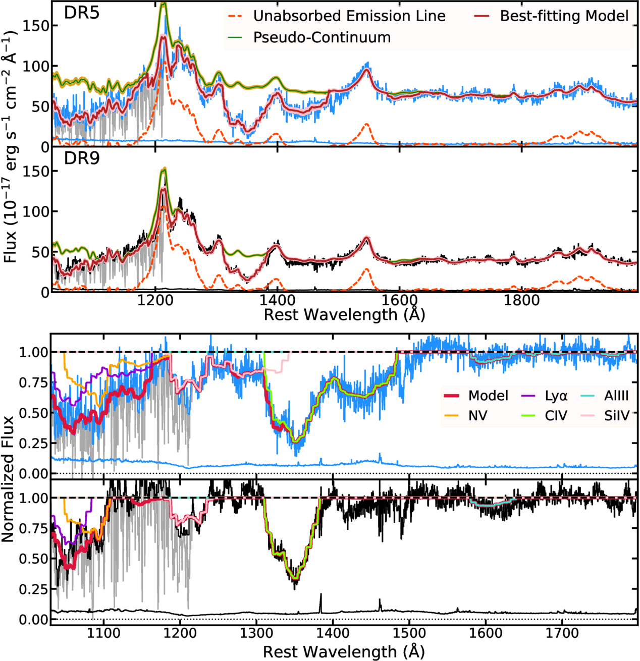
Figure 6. Top two panels: the best-fitting SimBAL models and uncertainties (red and pink, respectively) for SDSS DR5 (blue) and BOSS DR9 (black), plotted over the rest-frame wavelength range of 1050−2000 Å used in the modeling. Bottom two panels: the pseudo-continuum normalized models with the line identifications, shown over a zoomed-in range of 1050−1800 Å. Gray lines show the spectrum data that includes both the outflow BAL troughs and the Lyman forest absorption lines, and the black lines show the data we used for the SimBAL model fitting, where the non-BAL absorption lines have been flagged and ignored. The unabsorbed emission-line features (gold) reveal a large amount of unabsorbed flux in the Lyα + N v emission-line region (Section 3.1.2). The BAL trough extends to a lower velocity with greater width in the SDSS data. The model for BOSS shows a little opacity from low-ionization ions such as Al iii, indicating a high-column-density outflow.
Download figure:
Standard image High-resolution imageThe best-fitting models for J1646 have the following prescription:

where the power-law (or broken power-law for SDSS) continuum emission is absorbed by the outflow gas (IBAL) and the emission lines are not absorbed by the outflow gas (for our reasoning, please see Section 3.1.2). As described in K. M. Leighly et al. (2018), the SimBAL analysis begins with an initial manual fitting of the spectrum by adjusting the fit parameters to get the SimBAL model to roughly match the data. We began the fitting process with the visual inspection of the spectra to estimate the outflow velocity of the BAL in order to place the bins for modeling the absorption. Based on Figures 4 and 5, we determined that the C iv trough starts from near the O i/S ii emission lines and ends before the Si iv emission line for DR9 and before the C iv emission line for DR5. Due to their different widths, we used a 19-bin top-hat model to fit the troughs in the DR5 J1646 data and an 8-bin model for DR9 to fit the troughs in DR9. We kept the bin width and the velocity of the highest velocity bin the same between DR5 and DR9 spectral models so that we could directly compare the differences in the column density and covering fraction parameters between the two epochs as a function of velocity. The number of bins (or bin width) used in the top-hat model does not affect the robustness of the SimBAL model fits (K. M. Leighly et al. 2018).
For this object, the top-hat bins were constrained to have the same  and
and  across the velocities while allowing
  and
and  for each bin to freely vary to model the BAL features. However, we did not include density as a fit parameter because we do not have any density-sensitive diagnostic absorption lines (e.g., A. B. Lucy et al. 2014) that can be used to constrain the density from the model fitting; instead, we fixed the density parameter at
  . As mentioned, both epochs were fit simultaneously with all the absorption parameters shared between the spectral models for DR5 and DR9, except for the covering fraction parameter. However, the BAL feature observed in DR5 shows a much larger velocity width than in DR9, extending to lower velocities (Section 3.2.1). We assigned a separate
  parameter for the modeling of the lower-velocity portion of the BAL trough in DR5.
We used SimBAL to fit both the pseudo-continuum (emission lines + continuum) and the absorption lines together (Section 3.1.2). We ran SimBAL to obtain the converged Markov Chain Monte Carlo (MCMC) chain, and using this chain, we generated best-fitting models for both epochs and extracted posterior distributions of the parameters with which we obtained the physical properties of the outflows. The principal absorption lines found by the best-fitting SimBAL models are C iv, Si iv, N v, and Lyα. Visual inspection did not reveal low-ionization transitions in either spectrum (such as Mg ii and Al iii), but the best-fitting models found evidence for weak Al iii, indicative of a high-column-density wind (e.g., M. Bischetti et al. 2024).
The best-fitting model for DR5 shows a very broad absorption feature stretched from ∼1500 to ∼1180 Å (third panel from the top in Figure 6). The feature consists of blended C iv and Si iv that overlap between ∼1300 and ∼1350 Å. We experimented with a modified SimBAL model for DR5 with extra top-hat bins at the highest velocity end in order to test the possibility that the absorption corresponds completely to an ultra-wide trough of C iv. The converged model from this experiment showed no discernible differences from our best-fitting model; in other words, even when inputting a larger velocity of C iv to the test model, the parameters rearranged themselves to create Si iv opacity and only show significant opacity C iv in between ∼1300 and ∼1500 Å, identical to what we found in the best-fitting model. Therefore, we eliminate the possibility that the absorption is wider than presented in the best-fitting model.
In order to investigate how much Si iv opacity is hidden near the Lyα + N v emission line, we separated the emission lines and continuum emission from the best-fitting models (Figure 7). The model decomposition clearly shows deep Si iv troughs in the accretion disk continuum emission. In contrast, the best-fitting SimBAL models in Figure 6 only show a moderate amount of apparent Si iv opacity from the main EHVO. That is because the bottoms of the Si iv troughs have been filled in by the flux from the unabsorbed Lyα + N v emission line, making the apparent depths of Si iv troughs shallower. This type of behavior is also seen in objects with lower-velocity outflows, where Lyα + N v BAL is filled in by the emission lines (e.g., K. Leighly et al. 2019a; K. S. Green et al. 2023).
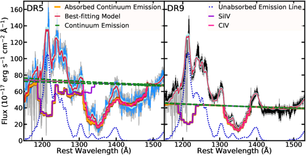
Figure 7. Si iv absorption identified by best-fitting SimBAL models in DR5 (left) and DR9 (right). A considerable amount of absorption from Si iv is seen in the continuum emission-only models, appearing much deeper than observed in Figure 6 due to strong Lyα + N v emission filling the bottom of the troughs (Section 3.2.2). The opacity profile of Si iv largely resembles that of C iv.
Download figure:
Standard image High-resolution image3.3. Measurements of Absorption
We also followed the two main approaches to characterizing and measuring the absorption. The AOD method serves as a lower limit and comparison to a more traditional method for the results obtained through SimBAL. One of the main differences is that the constraints from the AOD method are obtained from the C IV BAL features alone, whereas SimBAL spectral modeling takes into account the entire wavelength range.
3.3.1. AOD Approach: Measuring Absorption below Continuum Using Integrated Quantities and the AOD Method
Table 2 shows the integrated absorption measurements for both SDSS DR5 and BOSS DR9 epochs. We measured the balnicity index (BI; R. J. Weymann et al. 1991) modified to the EHVO (BIEHVO) by setting the integral limits to account for absorption between 30,000 and 60,000 km s−1, but we kept the parameter C to account for absorption larger than 2000 km s−1 (see Paper I for more details). Besides the BIEHVO, we also measured the BI using the original definition, setting the integral limits to be 5000 and 30,000 km s−1 (BIorig). Table 2 also includes EW values as the integration of the absorption within the total velocity limits and depth measurements, which were obtained by subtracting 1 minus the local averaged minimum flux value of the trough, as well as upper and lower-velocity limits for each EHVO, vmax,0.9 and vmin,0.9 respectively, which are determined by the wavelengths where the absorption crosses below the 90% of the normalized flux level. Values in Table 2 are rounded to reflect significant figures. Errors of BI, v , v
, v , EW, and depth are mostly influenced by the location of our continuum fit since it will shift the location of the normalized flux level; we estimated typical errors in Paper I by raising and lowering the normalized continuum by an amount that would place the new continuum fit within the spectrum error (typically by 5% of the normalized flux) and assigning the recalculated measurements as 3σ. We found these errors to be typically in the hundreds of kilometers per second: the BI and EWσ errors are less than ∼10% of their values, and typical v
 and v
and v errors are ∼200 km s−1; depth errors are ±0.02. All of our absorption measurements are carried out over the unsmoothed spectra, except for the depth value, as the smoothed spectra, where the noise is reduced, are a better representation of the actual depth.
Table 2. Absorption Measurements of J1646
| Epoch | BIorig | BIEHVO | EW | Depth | vmin,0.9 | vmax,0.9 |
|---|---|---|---|---|---|---|
| (km s−1) | (km s−1) | (km s−1) | (km s−1) | (km s−1) | ||
| DR5 | 0 | 6400 | 6800 | 0.72 | –34,100 | –50,200 |
| 2200 | ⋯ | 2400 | 0.34 | –15,100 | –28,300 | |
| DR9 | 0 | 3700 | 3900 | 0.61 | –36,000 | –49,000 |
Note. Typical BI and EW errors are less than ∼10% of their values (approximately hundreds of kilometers per second). Typical vmin,0.9 and vmax,0.9 errors are around ∼200 km s−1 and for depth errors are ∼±0.02. For DR5, the total quasar BI would be the sum of BIorig and BIEHVO.
Download table as: ASCIITypeset image
We find very large values of BI, both for the EHVO and the absorption at lower speeds. Based on the traditional BI definition, J1646 would be considered a BALQSO in the DR5 epoch but not in the DR9 one when this value is zero.
To obtain physical line measurements using the AOD method, we assumed that the line intensities at each velocity Iv are given by

where Io is the intensity of the continuum, Cf is the line-of-sight coverage fraction (0 ≤ Cf ≤ 1; see F. Hamann & G. Ferland 1999 for more information), and τv is the line optical depth. We assume τv to show a Gaussian profile dependent on the optical depth at the center of the line (τ0) and the Doppler parameter (b). Derived ionic column densities (Nion) were calculated as follows:

(B. D. Savage & K. R. Sembach 1991), where me and e are the mass and charge of the electron, respectively, and f is the oscillator strength of the ionic transition at λ0. The red line of the doublet is used to avoid potential saturation. Total column density, NH, values are derived from these Nion using a median value for the C iv ion fraction found in photoionization calculations (f(C iv) = −1.25; see Appendix in F. Hamann et al. 2011). We assume solar metallicities (M. Asplund et al. 2009).
Given the width of the BAL profile in both epochs, the C iv doublet is blended, and the determination of Cf, τ0, and b is an undetermined problem, even more so due to the added possibility of fitting more than one single pair of Gaussian profiles. We explored several tests, allowing the coverage fraction Cf to vary (constrained to be within physical values) or remain fixed, as well as using one doublet or several, always fixing the velocity separation of the C iv doublet and the ratio of optical depths within the doublet (2:1). In our fits, we also masked the region where the C ii 1335 Å emission line seems to be present (−46,500 < v < −44,000 km s−1 in Figure 8), and in DR5 we do not consider the Si iv+O iv] emission line is absorbed.
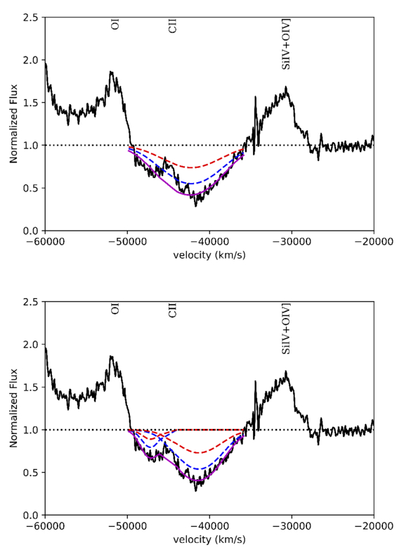
Figure 8. Examples of fitting results for the DR9 spectrum using our iterative approach (Methods 2 and 3 in Table 3). Method 2 (top): we use one pair of Gaussians for the C iv doublet. Method 3 (bottom): we use two pairs of Gaussians. In both cases, blue corresponds to C iv 1548 Å and red to C iv 1550 Å, and the combined fitting is indicated by the solid purple line. The region where C ii 1335 Å emission seems to be present (−46,000 < v < −44,000 km s−1) is masked in both fit inputs. Figures for DR5 are very similar, except for including another Gaussian pair for the lower-velocity absorption.
Download figure:
Standard image High-resolution imageTable 3 shows a summary of the AOD tests we used to measure the opacity:
- 1.Method 1: Fixing the Cf to be 1 and letting the central velocity v0, the width of the Gaussian b, and the central optical depth τ0 to vary.
- 2.Method 2: An iterative process where in Step (1) we fix Cf to be 1 and let b to vary as before,11 in Step (2) we then use the output b width as a fixed parameter for a fit where Cf are allowed to vary, and lastly, we repeat the first part of the iteration but using the output Cf from the previous step as the fixed parameter.
- 3.Method 3: A similar iterative process as Method 2, but allowing two pairs of Gaussians instead of one, fixing the Cf to be the same for both pairs, i.e., assuming that both gas clouds cover the same region of the quasar (see D. S. Rupke et al. 2005).
Table 3. Summary of AOD Fitting Methods Used in This Paper
| Method | Description |
|---|---|
| 1 | Fixing coverage fraction Cf to 1 |
| 2 | Iterativea |
| 3 | Iterativea,b with two pairs of Gaussians |
Notes.
aIterative meaning first fixing Cf = 1, then fixing b to the output of the previous iteration (all other parameters free), then fixing Cf to the output of the previous iteration (all other parameters free). bSame Cf for all pairs of Gaussians.Download table as: ASCIITypeset image
Table 4 and Figure 8 show the results of these fitting processes. Each line in Table 4 includes the measurement of one Gaussian pair. Figure 8 shows the fitting results for Methods 2 and 3 (the solid purple one) in DR9, where the doublets are indicated as blue/red lines (1548/1550 Å, respectively)—fittings in DR5 were similar except for adding another Gaussian pair for the lower-velocity absorption. Method 2 resulted in better constrained parameters, meaning smaller error values, for both DR5 and DR9, but the goodness of the fit was, as expected, better with Method 3; the standard deviation errors are derived from the covariance matrix of the fit. Both methods are limited by the fact that a single Cf was used for all velocities of the broad profile, and Method 3 has the additional limitation that the same Cf is assumed for both Gaussian pairs used in the C iv EHVO fitting. Given that our goal is to provide a good lower limit for the measurement and a smaller Cf results in a larger τ0 and therefore a larger column density, we will use the results of Method 3 as they provide slightly lower values of column densities.
Table 4. C iv Absorption AOD Fitting Results
| Epoch and Method | vmax,0.9 | vcentroid | Cf | b | τ0 |

|

|

|
|---|---|---|---|---|---|---|---|---|
| (km s−1) | (km s−1) | (km s−1) | (cm−2) | (cm−2) | (cm−2) | |||
| DR5 1 | –50,200 | –42,100 | 1.0 | 5780 ± 150 | 0.79 ± 0.03 | >16.30 | >21.12 | >21.25 |
| –28,300 | –22,800 | 1.0 | 7100 ± 500 | 0.258 ± 0.011 | >15.85 | >20.67 | ⋯ | |
| DR5 2 | –50,200 | –42,100 | 0.87 ± 0.06 | 5680 ± 150 | 1.00 ± 0.04 | >16.40 | >21.29 | >21.38 |
| –28,300 | –22,800 | 1.0a | 7100 ± 500 | 0.258 ± 0.011 | >15.85 | >20.67 | ⋯ | |
| DR5 3 | –50,200 | –47,400 | 1.00−0.14b | 1700 ± 300 | 0.40 ± 0.04 | >16.28 | >21.10 | >21.24 |
| ⋯ | –40,900 | 1.00−0.14b | 4700 ± 200 | 0.767 ± 0.025 | ⋯ | ⋯ | ⋯ | |
| –28,300 | –22,800 | 1.0a | 7100 ± 500b | 0.258 ± 0.011 | >15.85 | >20.67 | ⋯ | |
| DR9 1 | –49,000 | -42,700 | 1.0 | 4600 ± 100 | 0.60 ± 0.02 | >16.08 | >20.90 | ⋯ |
| DR9 2 | –49,000 | –42,700 | 0.85 ± 0.07 | 4500 ± 100 | 0.79 ± 0.03 | >16.20 | >21.02 | ⋯ |
| DR9 3 | –49,000 | –47,400 | 0.94 b
b
| 1500 ± 200 | 0.26 ± 0.02 | >16.09 | >20.91 | ⋯ |
| ⋯ | –41,600 | 0.94 b
b
| 3500 ± 100 | 0.69 ± 0.02 | ⋯ | ⋯ | ⋯ | |
Notes. AOD results of the C iv absorption measurements on the normalized spectra. The methods used in both spectra are described in Table 3. For each method, the results are included from the longest to the lowest absolute speed (in other words, the EHVO appears first). The best fits were found using Method 3 in both epochs.
aThe shape of the absorption at a lower velocity (vmax −28,300 km s−1) does not suggest the use of two pairs of Gaussians, and only Method 1 obtains good results. We include the measurement from Method 1 with a single pair. bBoth Cf are allowed to vary, but they are constrained to have the same value.Download table as: ASCIITypeset image
We find the results are consistent with full or close to full coverage (Cf ≃ 0.94−1.00), wide Gaussians (b ≃ 1500−7100 km s−1), and optical depths below 1τ ≃ 0.258−0.767. We find lower limits for the column densities  of 21.24 (cm−2) and 20.91 (cm−2) for DR5 and DR9, respectively. All results included in both tables are lower limits due to several reasons, including (1) we assumed that the O i and Si iv+ O iv] emission lines are unabsorbed, and thus absorption is restricted to areas below the normalized continuum away from emission, and (2) the measurements are carried out in the spectra normalized by a conservative method (see Section 3.1.1).
3.3.2. Best Estimate: Absorption Properties from SimBAL Models
We extracted the gas physical parameters  ,
,  , and the covering fraction parameter
  , as well as the gas kinematics (outflow velocity and width) of the BAL outflows from the best-fitting SimBAL models. We report the results extracted from the models in which the two spectra were fit simultaneously with gas density fixed at
  . The outflow properties constrained from the SimBAL models are tabulated in Table 5. Using the MCMC chains produced by SimBAL, we calculated the median values and 2σ uncertainties from the posterior distributions of each parameter.
Table 5. Absorption Measurements Extracted from SimBAL Models
| Epoch | vmax,0.9 | vmin,0.9 |

|
 a
a
|
 b,c
b,c
|
 c
c
|
 c (combined)
 |
|---|---|---|---|---|---|---|---|
| (km s−1) | (km s−1) | (cm−2) | (cm−2) | (cm−2) | |||
| DR5 | –48,500 | –34,200 | −0.7 ± 0.04 | 21.36−22.95 | 0.71−1.2 |

| 21.79 ± 0.06 |
| –34,200 | –14,300 |

| 21.59−23.04 | 1.19−1.78 |

| ⋯ | |
| DR9 | –48,500 | –34,200 | −0.7 ± 0.04 | 21.36−22.95 | 0.9−1.3 |

| ⋯ |
Notes.
aThe range of values estimated from the multiple bins is reported. bA large value of corresponds to a small covering fraction. cThe total outflow column density is the sum of the covering fraction-weighted column densities calculated for each bin. The parameters as a function of velocity are plotted in Figure 9.
Download table as: ASCIITypeset image
The EHVO trough for BOSS DR9 extends from −34,200 to −48,500 km s−1 with a remarkable velocity width of vwidth ∼ 14,300 km s−1. The SDSS DR5 revealed even more dramatic BAL that extends to a much lower velocity of −14,300 km s−1 with vwidth ∼ 34,200 km s−1. Similar to what was found for DR5 when using the scaled DR9 template (Section 3.1.1; see Figure 2), SimBAL also modeled the absorption in DR5 as a single continuous trough; however, the value of the highest velocity end of the trough identified by SimBAL is more comparable with the results from the AOD fitting for DR9, but slightly lower for DR5. From the best-fitting models, we obtain the ionization parameters of  for the high-velocity portion of the trough that is observed both in DR5 and DR9, and
  for the lower-velocity part of the BAL, only observed in the DR5 spectrum. We note that all absorption parameters, with the exception of the covering fraction parameter (
 ), for the high-velocity portion of the trough have been tied to be identical between epochs (Section 3.2.2). Additional SimBAL simulations were performed to assess the robustness of the ionization parameter constraints (Appendix B).
We calculated the total outflow column densities  (cm−2) and
  (cm−2) for DR5 and DR9, respectively. The total outflow column density is calculated by summing the covering fraction-weighted column densities calculated from each top-hat bin (Figure 9;
  ; N. Arav et al. 2005; K. M. Leighly et al. 2018, 2019b; H. Choi et al. 2022a). We excluded bins with negligible values (
 ) from the total column density calculation, as their uncertainty estimates were bound by the lowest values in the grid.
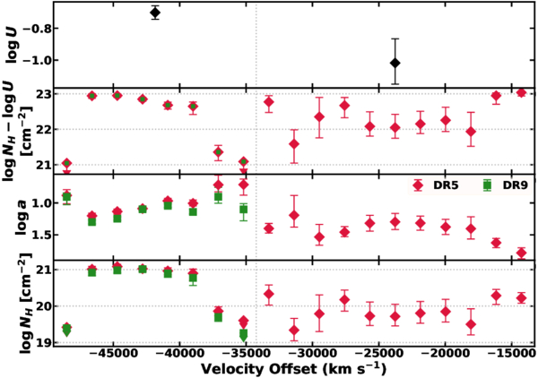
Figure 9. The outflow physical properties as a function of velocity from the top-hat models for SDSS DR5 and BOSS DR9 spectra. The outflow found in BOSS lacks the lower-velocity part of the outflow seen in the SDSS spectrum. The best-fitting models plotted here used a fixed value of  . The downward arrows represent the upper-limit estimates because of the finite sizes of the column density grids currently available in SimBAL.
Download figure:
Standard image High-resolution imageFigure 9 shows the physical properties of the outflow gas observed in DR5 and DR9 as a function of velocity determined from the best-fitting SimBAL models. We found consistently larger values of  and smaller values of
  for all bins in the model for the DR9 spectrum. The figure reports two ionization parameters constrained in the fitting, one for the high-velocity region in both DR5 and DR9 and the other for the lower-velocity region in DR5. We experimented with a set of models where we allowed
  to vary across the velocities; however, they did not produce sufficiently statistically better model fits to justify increasing the number of degrees of freedom and fit parameters of the models. As mentioned in Section 3.2.2, gas density was not constrained from the SimBAL fitting since there are no absorption lines in the bandpass that are sensitive to the change in density. Although there is neither information in the spectra with which we can estimate the density of the outflow gas nor other EHVO outflows with constrained gas densities,
  (cm−3) is a reasonable assumption for BAL outflow gas, and previous SimBAL analysis of a BALQSO SDSS J0850+4451 (K. M. Leighly et al. 2018) found similar density constraints. We further discuss the possible range of densities of the outflowing gas in J1646 and resulting wind properties in Section 4.2.1.
4. Summary and Discussion
J1646 shows very strong EHVO absorption profiles, resembling some of the strong BALs found at lower speeds. In the next section, we summarize the results found for its extreme outflow, and we discuss the implications of such an energetic outflow in the following ones.
4.1. Summary of Results Obtained with Both Methods
Using a combination of commonly used conservative methods and a state-of-the-art novel spectral synthesis code, we obtain measurements and very well-constrained lower and upper limits for the absorption parameters. We found absorption primarily and most strongly in C iv, accompanied by Lyα, N v, and Si iv absorption at the same speeds (see Figure 6).
Table 2 includes all speed measurements; typical errors are ∼200 km s−1. In the first epoch (DR5), the maximum outflow speed reaches vmax,0.9 = − 50,200 km s−1, slightly decreasing in the second epoch (DR9) to vmax,0.9 = −49,000 km s−1. Absorption at lower velocity is only present in the first epoch, so the minimum velocity of this outflow dramatically changes from vmin,0.9 = −15,100 km s−1 to vmin,0.9 = −36,000 km s−1. The location of the Si iv+O iv] emission line in the middle of the absorption profile in DR5 makes it more difficult to attribute the changes in that wavelength region to either the new presence of absorption or changes in the emission.
In this paper, we have presented the results using two different methods. The first method (AOD; Sections 3.1.1, 3.2.1, and 3.3.1) results in a very conservative lower limit of the absorption estimates: It allows us to estimate lower limits of column densities, as smaller coverage fraction Cf values will result in larger optical depths, and hence larger column densities. The second method (SimBAL; Sections 3.1.2, 3.3.2, and 3.3.2) provides the best estimate. It allows obtaining very good constraints of ionization  , the covering fraction parameter
  that models the inhomogeneous partial covering by using a power-law opacity distribution, as well as a good estimate of the column density.12
The absorption in the SDSS DR5 epoch appears overall to be stronger and wider than in the BOSS DR9 one. Using AOD (Section 3.3.1), we measure that Cf might be consistent with full coverage in the high-velocity absorber 1.00−0.14; we fix it to that value in the measurements of the low-velocity absorber since it cannot be well constrained. Measurements of widths, optical depths, and ionic column densities using this method are included in Table 4 (Method 3). For the EHVO, we measure a column density of  (cm−2). For the lower-velocity absorption, we find a shallower profile with smaller optical depths and a column density of
  (cm−2). Overall, we find a lower limit for the column density of the absorption in DR5 of
  (cm−2). Using SimBAL (Section 3.3.2), we are able to measure the amount of N v, Lyα, and Si iv absorption in the EHVO, which allows us to determine ionization values13
and the covering fraction parameter (see Table 5). Unlike other EHVO quasars in Paper I, J1646 shows stronger Lyα than N v. Using these measurements, we are able to constrain better the total NH, resulting in a column density of
(cm−2). Using SimBAL (Section 3.3.2), we are able to measure the amount of N v, Lyα, and Si iv absorption in the EHVO, which allows us to determine ionization values13
and the covering fraction parameter (see Table 5). Unlike other EHVO quasars in Paper I, J1646 shows stronger Lyα than N v. Using these measurements, we are able to constrain better the total NH, resulting in a column density of  21.79 ± 0.06 (cm−2).
In the BOSS DR9 epoch, the absorption is only present at high speeds and appears slightly weaker overall. Using AOD (Section 3.3.1), we obtain a Cf that remains consistent with full coverage 0.94 and a total column density of
  (cm−2) in our best-fitting method (Method 3 in Table 4). When using SimBAL (Section 3.3.2), we tied all absorption parameters between epochs except
  since it provided the best fit (see Section 3.2.2). Therefore, we find the same ionization for DR9 as in DR5 but different covering fraction parameters over the absorption profile (see Figure 9 for values at each velocity bin). Other ions (N v, Lyα, and Si iv) are still present in the same outflow, better constraining the total NH, which results in a column density of
  (cm−2), just slightly lower than in the DR5 epoch.
4.2. Physical Properties of J1646’s Outflow
4.2.1. Location of the Outflow
To estimate the mass outflow rate and the energy the outflow is carrying, we need to determine the location (radius) of the J1646 outflow. This radius (R) can be calculated using the definition of the ionization parameter, U = Q/4πR2nc, where the number of photoionizing photons per second emitted from the central engine (Q) can be estimated from the analysis of the broadband SED, while the density of the gas (n) and the ionization parameter (U) are constrained from detailed spectral analysis. We estimated  by scaling a standard quasar SED (SED used to create the SimBAL grids; K. M. Leighly et al. 2018) to match the J1646 photometry and then integrating the photon flux for energies larger than 13.6 eV. The SimBAL analysis provided us with excellent constraints on the ionization parameters and column densities of the outflowing gas observed in the spectra of J1646. However, due to the lack of density-sensitive diagnostic absorption lines in the spectra, it is not possible to directly constrain the density of the gas. This means we need to infer the location of the outflowing gas using our prior knowledge about BAL cloud geometry and the properties of spectral variability seen in this object.
Many previous studies (e.g., F. Hamann et al. 1997b; D. Narayanan et al. 2004; P. Rodríguez Hidalgo et al. 2011) derive location estimates from the absorption profile variability. Unfortunately, the time interval between the two observations is quite large, which results in a very high upper limit for the distance. If, as those studies do, we assume that the BAL variability is caused by a change in the ionization state of the outflowing gas, we can estimate the density of the gas using the equation, Δt > 1/neαr, where Δt is the BAL variability timescale, ne is the electron density of the gas (n in SimBAL), and αr is the recombination-rate coefficient (e.g., F. Hamann et al. 1995; D. M. Capellupo et al. 2013). We obtain ne > 103 (cm−3) with αr = 1.5 × 10⁻¹¹ (T = 20,000 K; S. M. McGraw et al. 2017) and Δt ∼ 1.7 yr (Section 2). This would put the outflowing gas in this object at r ≲ 1500 pc from the central SMBH. On the other hand, we can obtain a lower limit for the outflow location by considering the gas to be moving transversely; then, we can estimate the distance of the outflows with the equation,  , where R is the distance of the outflowing gas from the central SMBH, MBH is the mass of the SMBH, G is the gravitational constant, and vtrans is the transverse velocity of the clouds that can be approximated as Keplerian speed (D. M. Capellupo et al. 2011; E. A. Moravec et al. 2017). Although it is possible to derive an observation-based transverse velocity based on variability timescales, this method requires a higher cadence spectroscopic campaign to estimate a reliable transverse velocity (ideally more than two epochs that capture both the appearance and disappearance of the trough), which does not exist for J1646, as we mentioned above. We take the mass of the central SMBH in J1646
  (A. L. Rankine et al. 2020) and assume that the line-of-sight outflow velocity we measure from the shift of the BALs is the plausible upper limit of the transverse velocity vtrans ≲ 50,000 km s−1 (e.g., P. B. Hall et al. 2011). These values return R ∼ 0.006 pc, which is about 18 times the Schwarzschild radius (Rs ∼ 0.0003 pc).
To derive better upper and lower limits on the radius of the wind in J1646, we made assumptions about the energetics and physical properties of the EHVO winds based on our prior knowledge about BAL winds following the approach introduced in M. Bischetti et al. (2024). We estimated the lower limits of the BAL radius to be R ≳ 5−7 pc, conservatively assuming that a typical BAL outflowing gas has  , consistent with the range of gas densities found in previous work with SimBAL (K. M. Leighly et al. 2018; H. Choi et al. 2022b; K. S. Green et al. 2023) and using the equation for the ionization parameter above. However, we note that higher gas densities (
 ) have been reported in a few extreme BAL systems with Balmer line absorption (e.g., P. B. Hall et al. 2007; A. Schulze et al. 2018).14
The lower range value was calculated for the EHVO trough that was constrained to have a higher-ionization parameter (
) have been reported in a few extreme BAL systems with Balmer line absorption (e.g., P. B. Hall et al. 2007; A. Schulze et al. 2018).14
The lower range value was calculated for the EHVO trough that was constrained to have a higher-ionization parameter ( ) than the disappearing low-velocity trough.
The upper limit of the BAL radius was derived assuming that a steady BAL wind, which may be radiatively driven (e.g., K. Zubovas & A. King 2012; A. King & K. Pounds 2015), cannot transport energy greater than the radiative power of the quasar. The kinetic luminosity or power of the outflow is given by the equation,  . The mass outflow rate (
 ) can be calculated using the equation,
  (J. P. Dunn et al. 2010), where the mean molecular weight is assumed to be μ = 1.4. The global covering fraction (Ω) is estimated from the population statistics of typical (non-EHVO) BAL quasars. Assuming an expanding shell geometry of BAL winds, the fraction of outflowing gas covering the entire solid angle is expected to correspond to the fraction of the quasar population that shows BAL features. Given the lack of information about the fraction of EHVO quasars among the quasar population, an accurate estimate of the EHVO global covering fraction is not available. Therefore, we assumed that the EHVOs share a similar outflow geometry as non-EHVOs and used the Ω = 0.2, typically adopted for BAL winds (e.g., P. C. Hewett & C. B. Foltz 2003). A smaller covering fraction would result in a lower value for the mass outflow rate proportionally. Notice that while the kinetic luminosity is proportional to the radius of the outflow, it is more strongly dependent on the velocity of the outflow, as it is proportional to v3.
We estimated the upper limits of the outflow radius for the EHVO at R ≲ 30 pc, the values at which the kinetic luminosity of the outflow approaches the quasar luminosity LKE ∼ Lbol for DR5 and DR9, respectively. The small difference in the plausible upper limits is due to the lower outflow column density in DR9 BAL. For the lower-velocity BAL, a significantly larger upper limit of R ≲ 540 pc can be assumed, as the lower outflow velocity permits R to reach higher values before the kinetic luminosity matches the quasar luminosity. These upper limits correspond to the gas density of  . Figure 10 summarizes the process by which we obtained the plausible range of radii of the outflows seen in J1646.
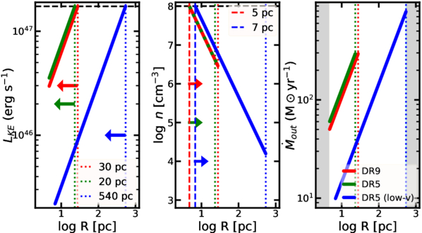
Figure 10. Left panel: the kinetic luminosity of the outflow as a function of the plausible range of distances of the outflow from the central SMBH. The dashed horizontal black line represents Lbol, which we considered as the upper limit for outflow power. The arrows represent the upper limits on  , which were set by assuming LKE ≲ Lbol for DR5 (low-v; blue), DR5 (EHVO, green), and DR9 (EHVO, red). Middle panel: the range of gas densities corresponds to the range of distances of the outflow from the central SMBH. The dashed horizontal black line represents the upper limit on gas density,
  , that we assumed to estimate the lower limits on the radii of BAL outflows, which are shown as vertical dashed lines and arrows. Right panel: the mass outflow rates of the BAL outflows as a function of the plausible radii of BAL outflows.
Download figure:
Standard image High-resolution imageWe conservatively estimate that the outflowing gas for the EHVO, which we observe in both epochs, is likely located at 5 ≲ R ≲ 30 pc, and the low-velocity BAL, only present in DR5, is likely at 7 ≲ R ≲ 540 pc away from the central engine. It can be seen that a much smaller range of R is obtained for the EHVO due to its high outflow velocity, restricting the plausible location of the outflow gas much closer to the central SMBH. We stress that our results do not explicitly preclude the possibility that the gas clouds creating the high-velocity and low-velocity troughs could be at the same location in the quasar. The difference in constrained  values between the high- and low-velocity troughs is marginal, given their uncertainties. Furthermore, we conducted an additional suite of SimBAL simulations using a single
  parameter to fit the entire trough observed in DR5. The results indicated that a
  provided a satisfactory fit across both the EHVO and low-velocity BAL regions, consistent with the constraints extracted from the best-fitting model for the EHVO trough. In other words, it is possible that a single gas cloud (or a group of cloudlets) produced the wide BAL features observed in DR5, and the change in geometry or spatial distribution of the gas relative to the line of sight caused the lower part of the BAL trough to be absent in DR9. We discuss in detail the potential scenarios for the variability in Section 4.3.3.
Even higher (lower) density will place the gas unrealistically too close (far) from the central SMBH, which has not been observed in BAL quasars (e.g., K. M. Leighly et al. 2018; H. Choi et al. 2022a, 2022b). Robust detections of outflows within the broad-line region (BLR) remain elusive. While large radii of BAL winds have been discovered (e.g., R ∼ 10s kpc; D. Byun et al. 2022), the extremely high outflow velocities found in J1646 disfavor such a large-scale expanding shell scenario, as it would result in the unrealistically high kinetic luminosity of the wind and challenge current models of wind acceleration at large radii (e.g., C.-A. Faucher-Giguère & E. Quataert 2012; C.-A. Faucher-Giguère et al. 2012).
Although it is difficult to further narrow the range of expected locations of the outflowing gas, we can assume that the actual location of the outflowing gas may be closer to the lower bound of the range. This is because we observe unabsorbed emission lines present within the absorption-line profile: Si iv+O iv] in the DR5 epoch, resembling the shape of the emission lines in the later epoch, and C ii in both epochs. We showed that the emission lines, in general, are very similar in both epochs (see Section 3.1.1), and our best-fitting SimBAL model included them also unabsorbed (Section 3.1.2). Such differential partial covering between line emission and continuum emission is difficult to produce with gas clouds located at a large distance because the angular sizes of the emission sources become extremely small (e.g., K. M. Leighly et al. 2019b; H. Choi et al. 2022a), even if the gas is porous/patchy and the emission is not in our line of sight. However, this possibility cannot be ruled out, as it is well established that the BLR does not fully cover the central SMBH (ΩBLR ≲ 0.2; e.g., K. M. Leighly 2004); otherwise, all X-ray spectra would be significantly absorbed. BAL outflowing gas also covers a portion of the central engine (ΩBAL ∼ 0.2; e.g., P. C. Hewett & C. B. Foltz 2003), though there is no requirement that ΩBLR and ΩBAL cover the same solid angle. Similar differential partial covering, in which line emission appeared unabsorbed by BAL outflows, has been reported in several FeLoBAL quasars (e.g., X.-H. Shi et al. 2016; H. Choi et al. 2022b) with similar bolometric luminosities ( ). They reported that the BAL outflowing gas is located at distances ranging from approximately parsec to ∼10 pc from the central SMBH, which are greater than the assumed size scales of the BLR (RBLR ≲ pc). Such residual emission features at the bottom of BAL troughs are not uncommon (e.g., E. J. Wampler et al. 1995) and are likely caused by multiple factors, including partial coverage of the BLR by BAL gas (e.g., K. M. Leighly et al. 2019b) and scattering of BLR emission by dust (e.g., P. M. Ogle et al. 1999; H. Choi et al. 2020).
The radius of the BLR can be estimated from the monochromatic flux at 5100 Å (M. C. Bentz et al. 2013) and appears to be around  pc for J1646. While we measure radial speeds, if we assume a correlation between the radial component and the total outflow velocity, it would be reasonable to conclude that EHVOs must be closer to the source than other typical BAL outflows at lower speeds. In fact, the best estimates of the location of ultra-fast outflows (UFOs) relative to the central source place them at a distance of 5Rs. For all these reasons, we expect the BAL outflow in J1646 to be located tens of parsecs from the central SMBH.
If the outflow in J1646 is located close to the central SMBH, Figure 10 shows that the density should be quite high for all absorbers. A higher density leads to a lower volume filling factor, presenting a greater challenge for explaining BAL cloud confinement (e.g., H. Choi et al. 2022a). For a fixed density, the EHVOs show a slightly smaller distance (R) than the lower-velocity absorber, so we might be seeing different parts of the outflow path.
Using the nominal speed of −50,000 km s−1, the outflow would have traveled just ∼0.09 pc in the quasar rest frame between the two epochs, so we can assume a similar location in the two epochs, provided the cloud is long lasting.
4.2.2. Mass, Energy, and Acceleration Mechanism of the Outflow
In Section 4.2.1, we calculated the mass outflow rates and the kinetic luminosities of the outflows using the properties constrained by the SimBAL analysis to derive a plausible range of location of the outflows (Figure 10). For the EHVO troughs that are present in both epochs, we estimated the mass outflow rate  and
and  for DR5 and DR9, respectively, corresponding to the range of 5 ≲ R ≲ 30 pc. The range of mass outflow rates for the BAL in DR9 extends to slightly lower values due to the lower column density (Table 5). We estimated the kinetic luminosity of
  .
.
The low-velocity component is estimated to have a mass outflow rate of  and a kinetic luminosity of
  . As mentioned above, we assumed the upper limit for the kinetic luminosity as the bolometric luminosity of the quasar,
  . If the outflowing gas clouds for the two velocity components are located co-spatially, the bulk of the outflow energy and mass would be mainly transported by the high-velocity component, given that the outflow strengths strongly depend on the outflow velocity,
  . We reiterate that the kinetic luminosity and the mass outflow rate of the outflow are both proportional to the assumed location of the outflow because we assume an expanding shell geometry. Combining both the low-velocity BAL and the EHVO components in DR5, assuming that they are physically independent of each other, we estimate a total mass outflow rate of
  and
and  for the total outflow power (see Table 6).
Table 6. Outflow Properties Calculated from SimBAL Results
| Epoch and BAL | R |

|

|
 a
a
|

|
|---|---|---|---|---|---|
| (pc) | (M⊙ yr−1) | (M⊙ yr−1) | (erg s−1) | (erg s−1) | |
| DR5, EHVO | 5−20 | 60−290 | 70−1080 | 46.6−47.2 | 46.6−47.5 |
| DR5, low-v BAL | 7−540 | 10−790 | ⋯ | 45.3−47.2 | ⋯ |
| DR9, EHVO | 5−30 | 50−290 | ⋯ | 46.5−47.2 | ⋯ |
Note.
aThe upper limits for the outflow kinetic luminosities were estimated to not exceed the quasar luminosity (LKE ≲ Lbol; see Section 4.2.1 and Figure 10).Download table as: ASCIITypeset image
The momentum flux ratio ( ;
;  ) can be used to infer potential outflow acceleration mechanisms of quasar outflows. For instance,
  is expected for radiatively driven winds in which the outflowing gas is accelerated by the scattering of photons (momentum conserving; e.g., A. King 2003; A. R. King & K. A. Pounds 2003). The ratio can exceed unity when dust is present in the gas cloud (T. A. Thompson et al. 2015). Quasar outflows with
  are also observed in ionized winds and molecular outflows (e.g., F. Fiore et al. 2017). These outflows are believed to be powered by an energy-conserving acceleration mechanism and are found mainly at large distances (
 (pc)) from the central SMBH (e.g., A. King & K. Pounds 2015). For J1646, we estimate
  and
and  for the high- and low-velocity troughs, respectively. Although these values are greater than unity, they are consistent with what has been observed in (FeLo)BAL outflows (e.g., F. Fiore et al. 2017; H. Choi et al. 2022b). While these simple calculations revealed no compelling observational evidence that special acceleration mechanisms are required to explain the EHVO’s extremely high velocity, further theoretical investigation is needed to better understand their acceleration.
4.3. Setting J1646 and Its Outflow in the Context of Other Quasars
4.3.1. Comparison to Other EHVOs and EHVO Quasars, and Other BALs and BALQSOs
The EHVO absorption feature in J1646 is rare in the sense that absorption observed at these speeds in UV/optical quasar spectra is not typically so wide and strong, showing such large EWs and depths. In Paper I, we found that, among the 6760 quasars sampled, none of the other 47 EHVO profiles discovered had equivalent widths or depths larger than the absorption feature found in the J1646 spectra. The second strongest profiles showed only 37% (EW = 2500 km s−1) or 80% (depth = 0.57) of the properties found in the BOSS DR5 spectrum of J1646, with most values much lower than 50%. J1646 also shows the largest width (Δv ∼ 16,100 km s−1). Similarly, other EHVO quasars in the literature (e.g., B. T. Jannuzi et al. 1996; P. Rodríguez Hidalgo et al. 2011) were observed to show weaker and narrower absorption. As a consequence, J1646 shows a larger Nion by more than 1 order of magnitude than the value found by P. Rodríguez Hidalgo et al. (2011) of Nion ∼ 0.8 × 1015 cm−2 for the C iv EHVO in PG0935+417.
Compared to measurements of other BALs (i.e., N. Filiz Ak et al. 2013), EHVOs show weaker troughs. Thus, it is natural that they tend to show relatively lower column density.15
Typical values of column densities found in BALQSOs are in the range  (K. M. Leighly et al. 2018, H. Choi et al. 2022b, K. S. Green et al. 2023; M. Bischetti et al. 2024, D. Byun et al. 2024), with FeLoBALs and LoBALs, showing larger values in general (F. Hamann et al. 2019). Compared to these studies, the column density of the wind in J1646,
  , is relatively low, largely consistent with its classification as a HiBAL, but we advise caution when comparing different classes, as the general properties of EHVO outflowing gas and HiBAL outflows remain poorly understood.
While the column densities for EHVOs are lower than those found in other BAL classes, their extreme speeds allow them to drive high-mass outflow rates and large kinetic luminosities. Indeed, the EHVO in J1646 represents one of the most powerful quasar outflows observed to date with  (LKE/Lbol ≳ 0.18). For comparison, H. Choi et al. (2020, 2022b) reported
  and the highest value of
  (which corresponded to LKE/Lbol ∼ 0.18) for a vBAL ∼−38,000 km s−1 wind found in a luminous FeLoBAL quasar at z ∼ 2.26 and a sample of low-redshift (z ∼ 1) FeLoBAL quasars analyzed using SimBAL, respectively. M. Bischetti et al. (2024) analyzed a high-redshift LoBAL quasar at z ∼ 6.6 using SimBAL to constrain an energetic wind with
  . This underscores the potential role of EHVOs in powering quasar feedback.
Even more, the measurements in J1646 might be underestimated. Several possibilities might be causing EHVOs to appear as weaker and shallower absorption profiles: (1) a small covering fraction, which is justified by (a) a Keplerian model where the fastest velocities would be observed closer to the SMBH, (b) our location estimates (see Section 4.2.1 and Figure 10), and (c) the large values of  obtained through the absorption profile with SimBAL16
fitting (see Figure 9); (2) incident spectral energy reduced by relativistic effects, which results in shallower profiles as the outflowing speeds increase (see A. Luminari et al. 2020). We describe these more in depth in our survey of EHVO quasars in DR16 (P. Rodríguez Hidalgo et al. 2025, in preparation).
obtained through the absorption profile with SimBAL16
fitting (see Figure 9); (2) incident spectral energy reduced by relativistic effects, which results in shallower profiles as the outflowing speeds increase (see A. Luminari et al. 2020). We describe these more in depth in our survey of EHVO quasars in DR16 (P. Rodríguez Hidalgo et al. 2025, in preparation).
In Paper I, we found that our sample of EHVO quasars in DR9 showed larger bolometric luminosities overall than the BALQSOs and non-BALQSOs in our parent sample. We have confirmed this result for the EHVO quasars in DR16 (P. Rodríguez Hidalgo et al. 2025, in preparation). However, among EHVO quasars alone, the properties of J1646 do not seem to make it an outlier, showing both a large bolometric luminosity and a large black hole mass, but a median value of the Eddington ratio. J1646 is a luminous quasar (g = 18.80 at MJD = 52760). EHVO quasars appear to show a distribution of larger values of bolometric luminosities compared to the parent sample, and J1646 lies within the top third or second quartile of other EHVO quasars in the Paper I sample, depending on the measurement.17 A. L. Rankine et al. (2020) measured a black hole mass of log(MBH/M⊙) = 9.5,18 and an Eddington ratio of log(Lbol/LEdd) = −0.4. The value of black hole mass situates it in the top quartile (median = 9.39, range = 8.90–9.58), but the Eddington ratio is very close to the median (median = −0.38, range = −0.72–0.09).
J1646 is also not an outlier relative to other quasars with EHVOs based on the properties of its C iv emission line. P. Rodríguez Hidalgo & A. L. Rankine (2022) carried out a study of the C iv emission-line parameter space for EHVOs in relation to BALQSOs and non-BALQSOs, finding that EHVOs show overall much larger values of C iv blueshift than the other two samples; this result has been confirmed when investigating a larger sample of EHVOs (L. Flores et al. 2025, in preparation). Among the EHVOs in P. Rodríguez Hidalgo & A. L. Rankine (2022), J1646 shows values close to median values with a C iv emission blueshift of ∼2470 km s−1 and a  of the C iv emission line of 1.334 Å. An additional way of representing this uses the value of the C iv distance (A. B. Rivera et al. 2020); for J1646, this value is 0.85, which also lies close to the median value of the EHVO distribution.
The strength of the He iiλ1640.42 emission line can be used as a proxy for the presence of soft X-ray continuum emission; D. A. Casebeer et al. (2006) showed that the He ii emission line is theoretically stronger for harder SEDs. Harder SEDs may overionize the gas, making it less likely to observe strong winds. Composites of BAL-type quasars have typically weaker He ii emission (G. T. Richards et al. 2011). In Paper I, the EW of the He ii emission line was measured in all of the EHVO quasars, following a similar procedure to A. Baskin et al. (2013, 2015). In J1646, He ii is embedded within the plateau of Fe ii emission lines redward of the C iv emission line, and is only clearly evident in the DR9 spectrum. Between the two epochs in J1646, we find that the absorption is weaker when the He ii emission appears stronger, as expected.
Finally, another way in which J1646 seems to differ from other EHVOs in our preliminary work (Paper I) is in the presence of Lyα as part of the outflow. J1646 is the only case in which Lyα seems similar or even stronger than N v. This result seems to be confirmed by the SimBAL fitting (see Figure 6). In Paper I, only five cases showed absorption at the wavelengths that would indicate Lyα, while 26 cases showed potential N v. Together with the presence of Si iv, it indicates this case is more optically thick than other EHVOs in our sample.
4.3.2. Comparison to UFO and X-Ray Observations
EHVOs are not the only outflows detected with such extreme speeds. UFOs have been observed as Fe K-shell absorption in the X-ray spectra of nearby AGN (predominantly Seyferts) at similar and even higher speeds (0.03c–0.4c; e.g., G. Chartas et al. 2002; F. Tombesi et al. 2010; and references therein). Because UFOs are searched for, mostly, in local AGN (zem < 0.1), the central engine shows typically moderate luminosities,  43–45.5 (erg s−1) (this was calculated as Lbol = kbolLion assuming a kbol of 10; see F. Tombesi et al. 2013). The upper limit of this range is still 2 orders of magnitude smaller than the value A. L. Rankine et al. (2020) found for J1646 (
 47.25 (erg s−1)). The detection of UFOs in high-z quasars is still rare, but if the trend between velocity and Lbol is extended to the X-ray absorbers, it might imply that UFOs in quasars with larger luminosities would show even larger velocities.
While we present our best value of column density and utilize it for the calculation of mass outflow rate, and thus outflow power, there are several indications that these results might still be underestimated. First, values of NH might be slightly underestimated in both methods, as we have not taken into account relativistic effects, as we discuss in Section 4.3.1. Second, there is a very limited number of studies of EHVOs observed in X-rays due to the redshifts of the quasars in which they are detected. In B. M. Sabra et al. (2003), a study of the quasar PG 2302+029, which presented an EHVO outflowing at ∼56,000 km s−1, showed that the column densities derived from the UV absorption lines did not surpass our values—their largest  was 15.7 (cm−2) derived from O vi, the
  measured for C iv was 14.9 cm−2. However, when observed in X-rays, they measured a column density from a related outflowing absorber that totaled
  22.4 (cm−2). If we also had an accompanying UFO, a 7 order of magnitude increase from our values would result in a column density of
  23–24 (cm−2).
In summary, assuming similar effects for UV/optical absorption as the effects in X-rays and that EHVOs are accompanied by ultra-fast X-ray absorbers, our results would be largely underestimated.
4.3.3. Comparison to Other SimBAL Variability Analyses
The simultaneous fitting using SimBAL of multiple epochs can provide information about the physical origin of the absorption variability. Because SimBAL allows the study of physical parameters for BAL outflows in great detail (e.g., physical properties as a function of velocity), we can investigate which physical change in the gas is responsible for the observed BAL variability. This analysis can be performed by investigating which parameter or a set of parameters can best model the spectroscopic time series data.
K. S. Green et al. (2023) used SimBAL in this manner for WPVS 007. They analyzed four epochs of HST Cosmic Origins Spectrograph spectra, revealing that changes in the covering fraction of the outflow gas ( ) were the primary driver of variability, rather than changes in ionization parameter or column density of the outflow. The key findings in their work indicate that this variability likely originated from structural changes within the outflowing gas itself rather than a transverse motion of the outflow gas, a common interpretation for BAL variability due to changes in partial coverage. They argued that changes in covering fractions are caused by the formation and dissipation of clumps of material along the line of sight with the use of
  in SimBAL, which models inhomogeneous power-law partial covering (M. de Kool et al. 2002; B. M. Sabra & F. Hamann 2005; K. M. Leighly et al. 2018). This representation of partial coverage can be interpreted as clumpy structures within the BAL outflow cloudlets (K. M. Leighly et al. 2019b), so that the changes in power-law partial covering may be interpreted as changes in the diffuseness of these clumps along our line of sight.
The multi-epoch spectra of J1646 were analyzed in a similar way to the approach taken by K. S. Green et al. (2023). As discussed in Section 3.2.2, we simultaneously fit the two epochs with SimBAL and allowed only a single parameter to vary to isolate the primary source of variability. This analysis revealed that the model that allowed covering fraction parameters to vary produced the best fits to the J1646 spectra, which is the identical model used for WPVS 007. Such results suggest that the EHVO variability seen in J1646 is also potentially caused by the changes in the sub-structures of the cloudlets that produce the absorption features (see Figure 11 in K. S. Green et al. 2023).
5. Conclusions
We perform the analysis of two-epoch spectra for the quasar J1646 (zem ∼ 3.04), to characterize the properties of its EHVO, observed in C iv, Si iv, N v, and Lyα, and remarkably variable between the two epochs separated ∼1.7 yr (rest frame), and the disappearing absorption at lower speeds. We approach the analysis in two ways: first, we employ a traditional method using AOD measurements, and second, we use SimBAL to perform simultaneous spectral fits. Here, we summarize the key results:
- 1.J1646 shows the widest and strongest absorption found in an EHVO to date. Its SDSS DR5 spectrum reveals a wide C IV BAL trough spanning from −50,200 to −15,100 km s−1. The BOSS DR9 spectrum shows a dramatic change in the C IV BAL, where the depth of the EHVO trough became weaker, and the range of velocities changed to −49,000 to –36,000 km s−1; this dramatic change at the lower end is due to the fact that the lower-velocity BAL disappeared altogether. J1646 also shows the only case in Paper I in which the absorption in Lyα seems similar or even stronger than N v. Together with the presence of Si iv, it indicates this case might be more optically thick, but analysis of the rest of the sample is necessary.
- 2.Using the conservative AOD approach described in Section 3.3.1, we measure optical depths for the EHVO of τ0 = 0.767 ± 0.025 and τ0 = 0.40 ± 0.04, and we find a coverage fraction Cf consistent with full coverage, which combined result on a lower limit for the ionic column density of
 16.28 (cm−2), and a column density of 21.10 (cm−2). For the low-velocity absorption, we find a shallower profile with smaller optical depths of τ0 ∼ 0.258 ± 0.011, an 15.85 (cm−2), and a column density of 20.67 (cm−2). Overall, we find a lower limit for the column density of the absorption in DR5 of 21.24 (cm−2). In the BOSS DR9 epoch, we obtain a Cf that remains consistent with full coverage (0.94), smaller optical depths of τ0 ∼ 0.69 ± 0.02 and τ0 ∼ 0.26 ± 0.02, a 16.09 (cm−2), and a total column density of 20.91 (cm−2). These results appear to be accurate lower limits relative to the results obtained with SimBAL below.
 - 3.We use SimBAL to simultaneously fit the multi-epoch spectra to constrain the outflow properties and investigate the physical origin of the variability. We obtain a best estimate for the outflow column density of (cm−2) for DR5 and (cm−2) for DR9. We find an ionization parameter for the EHVO in both epochs and for the lower-velocity BAL that is only present in DR5 (Section 3.3.2).
- 4.We estimate plausible ranges for the location of the outflow at 5 ≲ R ≲ 28 pc for the EHVO and 7 ≲ R ≲ 540 pc for the lower-velocity BAL absorber (see Section 4.2.1). Based on these estimates, we calculate the outflow power as for the EHVO and for the lower-velocity BAL, as well as mass outflow rates of in the first and Mout ∼50−290 M⊙ yr−1 in the second epoch for the EHVO, and for the lower-velocity BAL. The EHVO may be driving most of the mass outflow rate and kinetic luminosity, especially if the EHVO is cospatial or at larger distances than the lower-velocity outflow. Combined with its extreme speeds and the observation that several of these measurements might be underestimated, the EHVO in J1646 represents one of the most powerful quasar outflows observed to date, even when compared to LoBALs and FeLoBALs.
- 5.While EHVO quasars as a whole show distinct physical properties relative to BALQSOs and non-BALQSOs, we find that J1646 is not an outlier among other EHVO quasars (see Section 4.3.1). Its Eddington ratio (/LEdd = −0.4) is close to the median value of EHVO quasars, and its bolometric luminosity ( 47.25 (erg s−1)) is in the second quartile. Only its black hole mass ( 9.5 (M⊙)) is in the top quartile of those studied in Paper I. J1646 is also not an outlier in the C iv parameter space.
- 6.We investigate the potential origin of the dramatic variability observed between the two epochs in Section 4.3.3. The simultaneous multi-epoch fitting with SimBAL revealed that the changes in the covering fraction were the primary driver of BAL variability observed in J1646. This result is consistent with what has been found in the SimBAL analysis of WPVS 007 reported in K. S. Green et al. (2023).


All of these results underscore the crucial role of EHVOs in powering quasar feedback, the need to account for the energy carried by these outflows, and that further study is necessary to understand this type of quasar. Future surveys, such as SDSS-V, will provide key long-baseline spectral time series data that will further help us identify and study new variable EHVO quasars in greater detail.
Acknowledgments
P.R.H., M.M.C., and L.F. acknowledge support from the National Science Foundation AAG Award AST-2107960, funding provided by UW Bothell, and from the UW Royalty Research Fund A162630, as well as the Mary Gates Endowment through its research scholarships. Their work was partially supported by the SDSS’s Faculty and Student Team program, funded by the Alfred P. Sloan Foundation. H.C. and K.K.L. acknowledge support from the National Science Foundation AAG award Nos. AST-1518382, AST-2007023, and AST-2006771 to the University of Oklahoma. Support for SimBAL development and analysis is provided by NSF Astronomy and Astrophysics grant Nos. 1518382, 2006771, and 2007023. P.B.H. acknowledges support from NSERC grant 2023-05068. Funding for SDSS-III has been provided by the Alfred P. Sloan Foundation, the Participating Institutions, the National Science Foundation, and the US Department of Energy Office of Science. SDSS-III (www.sdss3.org/) is managed by the Astrophysical Research Consortium for the Participating Institutions of the SDSS-III Collaboration, including the University of Arizona, the Brazilian Participation Group, Brookhaven National Laboratory, Carnegie Mellon University, University of Florida, the French Participation Group, the German Participation Group, Harvard University, the Instituto de Astrofisica de Canarias, the Michigan State/Notre Dame/JINA Participation Group, Johns Hopkins University, Lawrence Berkeley National Laboratory, Max Planck Institute for Astrophysics, Max Planck Institute for Extraterrestrial Physics, New Mexico State University, New York University, Ohio State University, Pennsylvania State University, University of Portsmouth, Princeton University, the Spanish Participation Group, University of Tokyo, University of Utah, Vanderbilt University, University of Virginia, University of Washington, and Yale University. Some of the computing for this project was performed at the OU Supercomputing Center for Education & Research (OSCER) at the University of Oklahoma (OU). J.H.L. is funded through the Canada Research Chair program, as well as the Natural Sciences and Engineering Research Council of Canada (NSERC) Discovery and accelerator grant programs. The Université de Montréal recognizes that it is located on unceded (no treaty) indigenous territory, and wishes to salute those who, since time immemorial, have been its traditional custodians. The university expresses its respect for the contribution of indigenous peoples to the culture of societies here and around the world. The Université de Montréal is located where, long before French settlement, various indigenous peoples interacted with one another. We wish to pay tribute to these indigenous peoples, to their descendants, and to the spirit of fraternity that presided over the signing in 1701 of the Great Peace of Montréal, a peace treaty founding lasting peaceful relations between France, its Indigenous allies, and the Haudenosauni Confederacy (pronounced: O-di-no-sho-ni). The spirit of fraternity that inspired this treaty is a model for our academic community.
Appendix A: Identification of Lyα Forest Absorption
In order to be able to analyze the potential EHVO absorption present in the Lyα forest, we removed intervening Lyα absorption lines using the following method. We used an iterative sigma-clipping method to identify the pixels affected by the Lyα lines. Each iteration began with a smoothed spectrum made with a Gaussian kernel of a set width, followed by flagging all data points that fell a certain sigma (e.g., 0.5σ ∼ 2.5σ) below the smoothed spectrum. The subsequent iteration produced a new smoothed spectrum with the same Gaussian kernel but with an updated spectrum where the fluxes for the flagged data points from the previous iteration had been replaced by the interpolated values from the unflagged remaining data points. The iteration ended when no new data points were flagged. We experimented with Gaussian kernels of different widths and varying sigma cutoffs, and visually inspected the results to determine the best combination for our data. We flagged 49%/39% of the data points between 1030 and 1216 Å as affected by non-BAL absorption following our iterative method for the SDSS/BOSS spectrum. We tested different non-BAL absorption flags produced by various sigma cutoff values for the SimBAL fitting and found that the solutions from the best-fitting SimBAL models show no significant difference.
The use of this method is possible for BAL quasar spectra because the intrinsic absorption features from the outflows are broad and smooth, unlike the narrow absorption lines from the Lyα forest. Otherwise, the iterative sigma-clipping method would also flag the intrinsic absorption features along with the Lyα lines. We do not analyze the wavelengths shortward of 1030 Å because the sensitivity and S/N are reduced at the edge of the SDSS/BOSS spectrum, and an additional opacity from Lyβ absorption lines starts to contaminate the spectra, making it more difficult to estimate the quasar continuum.
Appendix B: Constraint of Ionization Parameter from SimBAL Modeling
In this appendix, we assess the impact of varying ionization parameter ( ) on the best-fitting SimBAL model and demonstrate the robustness of the derived constraint. We conducted an experiment in which we varied the ionization parameter by ±0.5 dex from the best-fitting parameters, fixed the ionization parameter, and then refit the spectrum. The results from this procedure are plotted in Figure 11, which shows how the best-fitting model evolves with these varies with ionization parameter. The most significant spectral variations occur in the N v/Lyα BAL complex. The strength of the N v absorption scales dramatically with the ionization parameter, resulting in an over- (under-) prediction of the opacity near ∼1100 Å when the ionization parameter is increased (decreased) from the best-fitting value. In contrast, the strength of the Lyα BAL responds to changes in the ionization parameter in the opposite direction and in a more subtle manner, with shallower absorption as the ionization parameter increases and slightly deeper absorption as it decreases. As a result, the N v transition predominantly controls the depth of the blended N v/Lyα BAL feature, providing a sensitive diagnostic that SimBAL leverages to robustly constrain the ionization parameter. While SimBAL performs exceptionally well in modeling heavily blended and saturated BAL troughs (Figure 6; e.g., H. Choi et al. 2020, 2022b), and we have effectively flagged the pixels affected by the Lyα forest (Appendix A), additional uncertainties in the derived outflow parameters may persist due to the N v/Lyα complex, which lies within this region. Future work involving a systematic analysis of EHVOs may further address and possibly clarify these issues (P. Rodríguez Hidalgo 2025, in preparation).
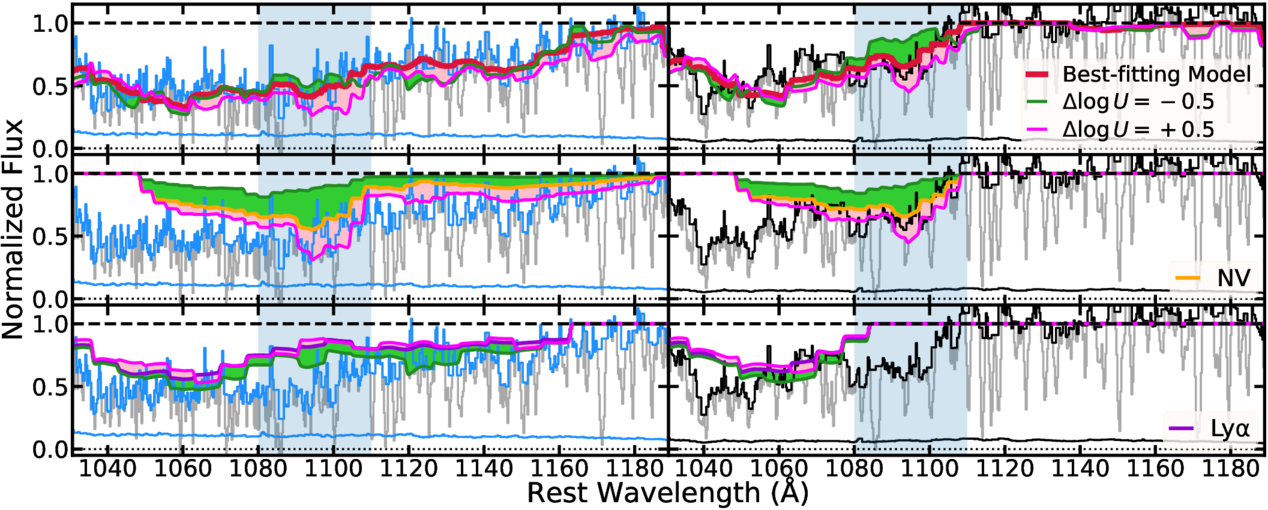
Figure 11. The top row shows how the best-fitting SimBAL models (red) change with varying ionization parameter ( ; green and pink), and the two bottom rows show the change in absorption strengths of Lyα and N v BALs with changing
  . We changed the ionization parameter by ±0.5 dex from the best-fitting values, fixed it, then refit the data to obtain the comparison SimBAL models. The spectra and their associated uncertainties for DR5 and DR9 are plotted in blue and black, respectively, in the left and right columns. The largest spectral variations occur around ∼1100 Å (blue-shaded regions), primarily driven by the substantial changes in the optical depth of N v, which scales with
  (middle row). Pixels affected by the Lyα forest, which have been masked (Appendix A), are shown in gray.
Download figure:
Standard image High-resolution imageFootnotes
- 8
Please note that throughout this paper, we will be calling BALs those broad absorption troughs at a lower velocity (<0.1c) than EHVOs, and BALQSOs the quasars that show BALs in their spectra.
- 9
- 10
R. R. Gibson et al. (2009a) incorrectly classified the EHVO C iv as “Si iv,” as is typically the case in previous surveys.
- 11
Both v0 and τ0 are variables through the whole Method 2, and the output of one step is used as the input of the following step.
- 12
Using the AOD method, we presented a scenario of very broad absorption that would be an upper limit of our estimates: The C iv absorption could extend from vmin = −13,900 km s−1 to vmax = −65,800 km s−1, but it is very uncertain where the potential Si iv or even N v absorption could be confused with C iv absorption. Therefore, we did not include the second scenario in our measurements as it is too unlikely and discouraged by the SimBAL method.
- 13
In the AOD method, we used a value of
–0.6, which resulted comparable to the value obtained with SimBAL for the EHVO: −0.7. - 14
There are several scenarios where the distance–density gas relationship would be more complex; for example, self-shielded gas where different strata of the gas receive a different influx of central radiation or patchy/compacted clouds of gas.
- 15
Note that J1646 was classified as a BALQSO based on the C iv absorption at lower speeds in DR5 (R. R. Gibson et al. 2009a). This absorption disappears in the DR9 observation, while the EHVO remains. As we have cautioned before, this classification based on one-time observations might not be optimal, as both EHVOs and BALs are known to be highly variable.
- 16
Increasing
corresponds to decreasing Cf (see, e.g., K. M. Leighly et al. 2019b). However, we note that inhomogeneous partial covering by and the homogenous (step-function) partial coverage using Cf assume different BAL cloud geometry, and therefore, a direct comparison between the two is not straightforward, as they represent distinct assumptions about the distribution and structure of absorbing material along the line of sight (e.g., K. M. Leighly et al. 2019b). Moreover, the values of were constrained by SimBAL using multiple BAL transitions, while Cf was derived by AOD solely from the C iv BAL trough. The two methods coincide on the direction of the change, as both of them show a reduction in partial coverage from measurements on DR5 to DR9. - 17
The value calculated by Y. Shen et al. (2011) for J1646 is Mi[z = 2] is −28.9 (MJD = 53167), which lies in the top third of values of the 21 quasars with EHVO that we studied in Paper I. The bolometric luminosity measured by A. L. Rankine et al. (2020) of log(Lbol/(erg s−1)) = 47.25 lies in the second quartile of values (median = 47.07, min = 46.58, and max = 47.55).
- 18


