Abstract
We report ALMA observations with resolution ≈05 at 3 mm of the extended Sgr B2 cloud in the Central Molecular Zone (CMZ). We detect 271 compact sources, most of which are smaller than 5000 au. By ruling out alternative possibilities, we conclude that these sources consist of a mix of hypercompact H ii regions and young stellar objects (YSOs). Most of the newly detected sources are YSOs with gas envelopes that, based on their luminosities, must contain objects with stellar masses
 . Their spatial distribution spread over a ∼12 × 3 pc region demonstrates that Sgr B2 is experiencing an extended star formation event, not just an isolated “starburst” within the protocluster regions. Using this new sample, we examine star formation thresholds and surface density relations in Sgr B2. While all of the YSOs reside in regions of high column density (
 ), not all regions of high column density contain YSOs. The observed column density threshold for star formation is substantially higher than that in solar vicinity clouds, implying either that high-mass star formation requires a higher column density or that any star formation threshold in the CMZ must be higher than in nearby clouds. The relation between the surface density of gas and stars is incompatible with extrapolations from local clouds, and instead stellar densities in Sgr B2 follow a linear
  relation, shallower than that observed in local clouds. Together, these points suggest that a higher volume density threshold is required to explain star formation in CMZ clouds.
1. Introduction
The Central Molecular Zone (CMZ) of our Galaxy appears to be overall deficient in star formation relative to the gas mass it contains (Güsten & Downes 1983; Morris & Serabyn 1996; Beuther et al. 2012; Immer et al. 2012; Longmore et al. 2013a; Barnes et al. 2017; Kauffmann et al. 2017a, 2017b). This deficiency suggests that star formation laws, i.e., the empirical relations between the star formation rate (SFR) and gas surface density, are not universal. The gas conditions in the Galactic center are different from those in nearby clouds, providing a long lever arm in a few parameters (e.g., pressure, temperature, velocity dispersion; Shetty et al. 2012; Kruijssen & Longmore 2013; Ginsburg et al. 2016; Henshaw et al. 2016; Immer et al. 2016) that facilitates measurements of the influence of environmental effects on star formation.
The CMZ dust ridge contains most of the dense molecular material in the Galactic center (Lis et al. 2001; Bally et al. 2010; Molinari et al. 2011). The observed star formation deficiency comes from comparing the quantity of dense gas to star formation tracers such as water masers and free–free emission (Longmore et al. 2013a), infrared source counts (Yusef-Zadeh et al. 2009), or integrated infrared luminosity (Barnes et al. 2017).
Recent searches for ongoing star formation using high-resolution millimeter observations of selected clouds in the CMZ have revealed few star-forming cores (Johnston et al. 2014; Rathborne et al. 2014, 2015; Kauffmann et al. 2017a, 2017b). As summarized by Barnes et al. (2017), most of the dust ridge clouds contain  of stars, or ∼2% of their mass in stars. The Sgr B2 N (North), M (Main), and S (South) protoclusters (Schmiedeke et al. 2016; labels are shown in Figure 1) are exceptional in that they are actively forming star clusters and contain high-mass young stellar objects (YSOs) and many compact H ii regions (e.g., Gaume et al. 1995; Higuchi et al. 2015); despite the active star formation, the overall cloud appears to be as inefficient as the other dust ridge clouds (Barnes et al. 2017). Besides Sgr B2, a few of the dust ridge regions are forming stars at a much lower level, including the 20 and 50
  clouds (Lu et al. 2015, 2017), Sgr C (Kendrew et al. 2013), and dust ridge Clouds C, D, and E (Ginsburg et al. 2015; Barnes et al. 2017; D. Walker et al. 2018, in preparation). These regions contain only a small number of high-mass cores, YSOs, and small H ii regions.
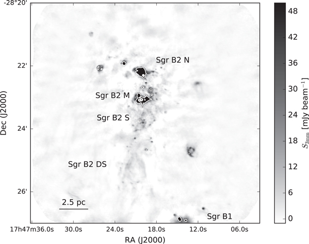
Figure 1. Overview of the Sgr B2 region, with the most prominent regions labeled. The image shows the ALMA 3 mm observations imaged with 15 resolution to emphasize the larger-scale emission features. White contours are included at [50, 500, 1000, 1500, 2000] mJy beam−1 to show the flux levels of the saturated regions. For a cartoon version of this figure, see Figure 1 of Schmiedeke et al. (2016).
Download figure:
Standard image High-resolution imageMost observations of the Sgr B2 cloud focus on the “hot cores” Sgr B2 N and M, which are high-mass protoclusters (they are likely to form clusters with M ≳ 104  ). The extended cloud has been the subject of some studies in gas tracers, but it has never been observed at high (
 ) resolution in the far-infrared or millimeter regime. Radio observations at
  have revealed extended
  and several masers (Martín-Pintado et al. 1999; McGrath et al. 2004; Caswell et al. 2010), but these tracers only detect a subset of star-forming sources. Martín-Pintado et al. (1999) suggested the presence of ongoing star formation in the broader Sgr B2 cloud based on the detection of three
  (4, 4) “hot cores” south of Sgr B2 S. Despite this suggestion and the high density of gas throughout the broader Sgr B2 cloud, an extended star formation event has not been verified.
We report the first observations of extended, ongoing star formation in the Sgr B2 cloud. We observed a  pc section of the Sgr B2 cloud and identified star formation along the entire molecular dust ridge known as Sgr B2 Deep South (DS, also known as the “Southern Complex”; Jones et al. 2012; Schmiedeke et al. 2016). These observations allow us to perform one of the best star-counting-based determinations of the SFR within the dense molecular gas of the CMZ.
We adopt a distance to Sgr B2  , which is consistent with Sgr B2 being located in the CMZ dust ridge. While Reid et al. (2009) measure a closer distance of 7.9 ± 0.8 kpc, and Boehle et al. (2016) measure a distance to Sgr A* of 7.86 ± 0.14 kpc, we use a value closer to the IAU-recommended Galactic center distance of 8.5 kpc, accounting for the distance difference of ≈100 pc measured by Reid et al. (2009).23
Choosing the closer distance would result in masses and luminosities smaller by 12%, which would not affect any of the conclusions of this paper.
, which is consistent with Sgr B2 being located in the CMZ dust ridge. While Reid et al. (2009) measure a closer distance of 7.9 ± 0.8 kpc, and Boehle et al. (2016) measure a distance to Sgr A* of 7.86 ± 0.14 kpc, we use a value closer to the IAU-recommended Galactic center distance of 8.5 kpc, accounting for the distance difference of ≈100 pc measured by Reid et al. (2009).23
Choosing the closer distance would result in masses and luminosities smaller by 12%, which would not affect any of the conclusions of this paper.
We describe the new ALMA observations and the archival single-dish data used to estimate gas column density in Section 2. We focus on the continuum sources selected from the ALMA data, which we identify in Section 3.1. In Section 3, we perform catalog cross-matching (Section 3.2) and classify the sources (Section 3.3). In Section 4, we discuss the SFR and flux distribution (Section 4.1), the relation between the clusters and the extended star-forming population (Section 4.2), and some implications of our observations for turbulent star formation theories (Section 4.5), and we examine star formation thresholds (Section 4.3) and surface density relations (Section 4.4). We conclude in Section 5. Afterward, several appendices describe the single-dish combination (Appendix A), self-calibration (Appendix B), and the photometric catalog (Appendix C). Three more appendices show additional figures of  (Appendix D), archival Very Large Array (VLA) 1.3 cm continuum data (Appendix E), and an additional comparison of the surface density relations to other works (Appendix F).
2. Observations and Data Reduction
2.1. ALMA Data
Data were acquired as part of ALMA project 2013.1.00269.S. Observations were taken in ALMA Band 3 with the 12 m Total Power array, with the ALMA ACA 7 m array, and in two configurations with the ALMA 12 m array; durations and dates of the observations and details of the array configurations are listed in Table 1. The setup included the maximum allowed number of channels, 30,720, across four spectral windows in a single polarization; the single-polarization mode was adopted to support moderate spectral resolution (∼0.8  , 244 kHz channels) across the broad bandwidth. The basebands were centered at 89.48, 91.28, 101.37, and 103.23 GHz with bandwidth 1.875 GHz (total 7.5 GHz). The off position used to calibrate the system temperature for the Total Power (TP) observations was at J2000 17:52:06.461, –28:30:32.095.
Table 1. Observation Summary
| Date | Array | Observation Duration | Baseline Length Range | No. of Antennas |
|---|---|---|---|---|
| (s) | (m) | |||
| 2014 Jul 01 | 7 m | 4045 | 9–49 | 10 |
| 2014 Jul 02 | 7 m | 4043 | 9–49 | 10 |
| 2014 Jul 03 | 7 m | 7345 | 9–48 | 8 |
| 2014 Dec 06 | 12 m | 6849 | 15–349 | 34 |
| 2015 Apr 01 | 12 m | 3464 | 15–328 | 28 |
| 2015 Apr 02 | 12 m | 3517 | 15–328 | 39 |
| 2015 Jul 01 | 12 m | 3517 | 43–1574 | 43 |
| 2015 Jul 02 | 12 m | 10598 | 43–1574 | 42 |
| 2015 Jan 25 | TP | 6924 | ⋯ | 3 |
| 2015 Apr 01 | TP | 1986 | ⋯ | 2 |
| 2015 Apr 11 | TP | 6920 | ⋯ | 3 |
| 2015 Apr 12 | TP | 10441 | ⋯ | 3 |
| 2015 Apr 25 | TP | 13928 | ⋯ | 3 |
| 2015 Apr 26 | TP | 22562 | ⋯ | 3 |
| 2015 May 18 | TP | 8342 | ⋯ | 3 |
Download table as: ASCIITypeset image
The ALMA QA2 calibrated measurement sets were combined to make a single high-resolution, high dynamic range data set. We imaged the continuum jointly across all four basebands (without excluding any spectral line regions) using CASA (version 4.7.2-REL r39762) tclean and found that the central regions surrounding Sgr B2 M were severely affected by artifacts that could not be cleaned out. We therefore ran three iterations of phase-only self-calibration and two iterations of amplitude+phase self-calibration, the latter using multiscale multifrequency synthesis (MTMFS) with two Taylor terms (Rau & Cornwell 2011), to yield a substantially improved image (see Appendix B). The total dynamic range, measured as the peak brightness in Sgr B2 M to the rms noise in a signal-free region of the combined 7 m+12 m image, is 18,000 (average rms noise 0.09 mJy beam−1, 0.05 K), while the dynamic range within one primary beam (05) of Sgr B2 M is only 5300 (average rms noise 0.3 mJy beam−1, 0.16 K). Because of the dynamic range limitations and an empirical determination that clean did not converge if allowed to go too deep, we cleaned to a threshold of 0.1 mJy beam−1 over all pixels with
 as determined from a previous iteration of tclean. The final image used for most of the analysis in this paper was imaged with Briggs robust parameter 0.5, achieving a beam size 0
54 × 0
46. Using the same visibility data, we also produce an image with robust parameter −1, beam size 0
37 × 0
32, and average rms 0.24 mJy beam−1 or 0.27 K, and another tapered to exclude the long baselines imaged with robust parameter 2 that achieved a beam size 2
35 × 1
99 with average rms 0.78 mJy beam−1 or 0.022 K. All three images are distributed with the paper [doi:10.11570/17.0007]. A degraded-resolution image with 1.5 arcsec resolution is shown to provide an overview of the region in Figure 1.
We also produced full spectral data cubes. These were lightly cleaned with a maximum of 2000 iterations of cleaning to a threshold of 100 mJy beam−1. The noise is typically ≈9 mJy  (6 K) per 0.8
  channel in the robust 0.5 cubes. No self-calibration was applied, both because the dynamic range limitations were less significant and because the image cubes are computationally expensive to process. Before continuum subtraction, dynamic-range-related artifacts similar to those in the continuum images were present, but these structures are nearly identical across frequencies and were therefore removable in the image domain. We use median-subtracted cubes (i.e., spectral cubes with the median along each spectrum treated as continuum and subtracted) for our analysis of the lines, noting that the only location in which an error
  on the median-estimated continuum is expected is the Sgr B2 north core (Sánchez-Monge et al. 2017, 2018). While many lines were included in the spectral setup,24
only
on the median-estimated continuum is expected is the Sgr B2 north core (Sánchez-Monge et al. 2017, 2018). While many lines were included in the spectral setup,24
only  J = 10−9 is discussed here; of the included lines, it is the brightest and most widely detected in emission. This line has a critical density
  (Green & Chapman 1978), so it would traditionally be considered a high-density gas tracer.
The processed data are available from [doi:10.11570/17.0007] in the form of four ∼225 GB data cubes for the full data sets, three continuum images at different resolutions, and two cubes of  at different resolutions.
2.2. Other Data—Column Density Maps
We use archival data to create column density maps at a coarser resolution than the ALMA data, since the ALMA data are not sensitive enough to make direct column density measurements and because they may be contaminated by other (nondust) emission mechanisms. We use Herschel Hi-Gal data (Molinari et al. 2010) to perform spectral energy distribution (SED) fits to each pixel (Battersby et al. 2011; C. Battersby et al. 2018, in preparation). These fits were performed at 25″ resolution, using the 70, 160, 250, and 350  data and excluding the 500
  channel. The estimated fit uncertainty in the column density is 25%, with an upper limit on the systematic uncertainty of a factor of two (C. Battersby et al. 2018, in preparation). To obtain column density maps with greater resolution, we combine the Herschel data with SHARC 350
  and SCUBA 450
  images.
The CSO SHARC data were reported in Bally et al. (2010) and have a nominal resolution of 9″ at 350  ; however, at this resolution, the SHARC data display a much higher surface brightness than the Herschel data on the same angular scale. An assumed resolution of 11
5 gives a better surface brightness match and is consistent with the measured size of Sgr B2 N in the image. This calibration difference is likely to have been produced by a combination of flux calibration errors and issues that increase the effective beam size, such as blurring by pointing errors, surface imperfections, and the gridding process. In any case, the Herschel data provide the most trustworthy absolute calibration scale, since they were taken from space and calibrated to an absolute scale using Planck data (Bendo et al. 2013; Bertincourt et al. 2016), so we assume that the Herschel calibration is correct when combining the data.
The JCMT SCUBA 450  data were reported in Pierce-Price et al. (2000) and Di Francesco et al. (2008) with a resolution of 8″. We found that the SCUBA data had a flux scale significantly discrepant from the Herschel-SPIRE 500
  data on 30″–90″ scales, even accounting for the central wavelength difference. We had to scale the SCUBA data up by a factor of ≈3 to make the data agree with the Herschel-SPIRE images on these scales. While such a large flux calibration error seems implausible, it can occur if the beam size of the ground-based data is larger than expected. To assess this possibility, we fit 2D Gaussians to several sources in the SCUBA CMZ maps, measuring an FWHM toward Sgr B2 N of approximately 14″ (and toward several other sources,
  ), which means that the observed beam area is about three times larger than theoretically expected. Between the larger beam area, flux calibration errors (quoted at 20% in Pierce-Price et al. 2000), and the dust emissivity correction (35%–50% for dust index
  , where
  ), this large
  flux scaling factor is plausible. The large secondary error beam (17
3; Di Francesco et al. 2008) of the 450
 SCUBA data may also contribute to this effect. As with the SHARC data above, we trust the space-based calibration over the ground-based one.
We combined the Herschel data with the SHARC and SCUBA data to create higher-resolution maps at 350  (Herschel-SPIRE+SHARC) and 450
  (Herschel-SPIRE+SCUBA). The data combination process is discussed in detail in Appendix A, but in brief, we used a “feathering” technique (e.g., Stanimirovic 2002; Cotton 2017, as implemented in uvcombine25
) to combine the images in the Fourier domain.
(Herschel-SPIRE+SCUBA). The data combination process is discussed in detail in Appendix A, but in brief, we used a “feathering” technique (e.g., Stanimirovic 2002; Cotton 2017, as implemented in uvcombine25
) to combine the images in the Fourier domain.
Using these higher-resolution maps, we created several column density maps using different assumptions about the dust temperature. For simplicity, we produced maps assuming arbitrary constant temperatures equal to the minimum and maximum expected dust temperatures (20 and 50 K). We produced additional maps using the temperature measured with Herschel SED fits interpolated onto the higher-resolution SCUBA and SHARC grids. Because of the interpolation and fixed temperature assumptions, the column maps are not very accurate and should not be used for systematic statistical analysis of the column density distribution (i.e., probability distribution function shape analysis) without careful attention to the large implied uncertainties. However, these higher-resolution data are used in this paper to provide the best estimates of the local column density around our sample of compact millimeter continuum sources.
One important uncertainty in these column density maps is possible foreground or background contamination. Sgr B2 is  away from us in the direction of our Galaxy’s center, meaning that there is a potentially enormous amount of material unassociated with the Sgr B2 cloud along the line of sight. This material may have column densities as low as
  or as high as
  , as measured from relatively blank regions in the Herschel column density map (Battersby et al. 2011; C. Battersby et al. 2018, in preparation). The former value corresponds to the background at high latitudes,
  , while the latter is approximately the lowest seen within our field of view.
3. Analysis of the Continuum Sources
In this section, we identify continuum sources (Section 3.1), match them with other catalogs (Section 3.2), and discuss their nature (Section 3.3).
3.1. Continuum Source Identification
We selected compact continuum sources by eye, scanning across images with different weighting schemes (different robust parameters). An automated selection is not viable across the majority of the observed field for several reasons:
- 1.There are many extended H ii regions that dominate the overall map emission. These are clumpy and have local peaks that would dominate the identified source population using most source-finding algorithms.
- 2.There are substantial imaging artifacts produced by the extremely bright emission sources in Sgr B2 M (
 ) and Sgr B2 N () that make automated source identification particularly challenging in the most source-dense regions. These are “sidelobes” from the bright sources that cannot be entirely removed.
 - 3.Resolved-out emission has left multiscale artifacts throughout the images. While these can be filtered out to a limited degree by excluding large angular scales (short baselines), there remain small-scale ripples, and the noise increases when baselines are excluded.


All of these features are evident in Figures 2 (with a higher-resolution inset version in Figure 3) and 4 (with a higher-resolution inset version in Figure 5).
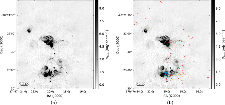
Figure 2. Images of the ALMA 3 mm continuum in the Sgr B2 M and N region. The right figure additionally includes markers at the position of each identified continuum pointlike source: red circles are “conservative,” high-confidence sources; orange squares are “optimistic,” low-confidence sources; cyan circles are H ii regions; magenta plus signs are  masers; blue plus signs are H2O masers; and green crosses are X-ray sources. The massive protocluster Sgr B2 M is the collection of H ii regions and compact sources in the lower half of the image. The other massive protocluster, Sgr B2 N, is in the center. The crowded parts of the images are shown with inset zoom-in panels in Figure 3.
Download figure:
Standard image High-resolution image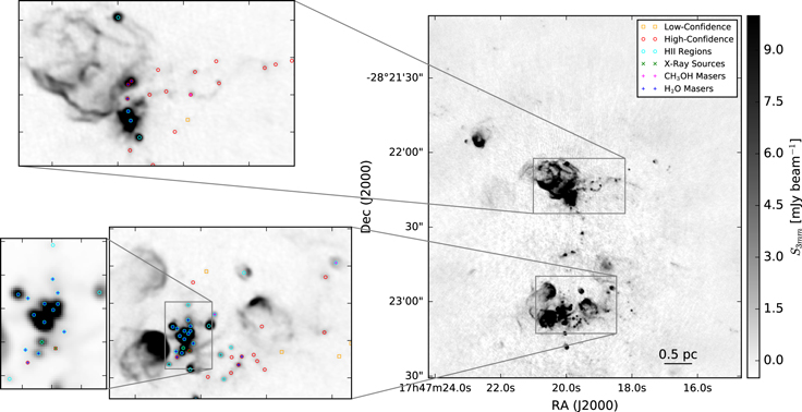
Figure 3. Close-in look at the Sgr B2 M and N region. Multiple insets show identified sources in some of the richer subregions. The points are colored as in Figure 2. The background image is the ALMA 3 mm continuum. See also Figure 22.
Download figure:
Standard image High-resolution image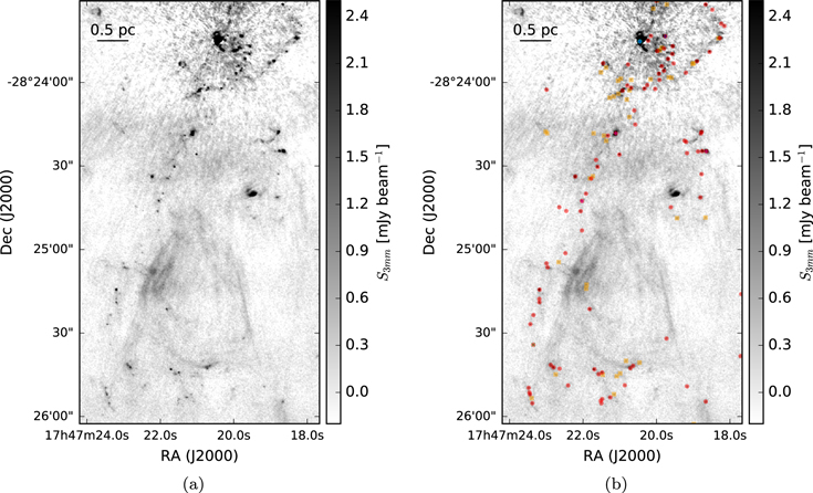
Figure 4. Images of the ALMA 3 mm continuum in the Sgr B2 Deep South (DS) region. The right panel additionally includes markers at the position of each identified continuum pointlike source: red circles are “conservative,” high-confidence sources; orange squares are “optimistic,” low-confidence sources; cyan circles are H ii regions; magenta plus signs are  masers; blue plus signs are H2O masers; and green crosses are X-ray sources. The H ii region Sgr B2 S is the bright source at the top of the image; imaging artifacts can be seen surrounding it. The largest angular scales are noisier than the small scales; the
  -wide east–west ridge at around −28:24:30 is likely to be an imaging artifact. By contrast, the diffuse components in the southern half of the image are likely to be real. The crowded parts of the images are shown with inset zoom-in panels in Figure 5.
Download figure:
Standard image High-resolution imageBecause the noise varies significantly across the map (it is higher near Sgr B2 M), and because there is extended emission, a uniform selection criterion is not possible. We therefore include two levels of source identification: “high-confidence” sources, which are peaks clearly above the noise in regions of low background, and “low-confidence” sources, which have somewhat lower signal-to-noise ratio and are often in regions with higher background in which the noise estimate may be inaccurate. The difference between the high- and low-confidence sources is subjective, since it is based in part on a by-eye assessment of how much the local noise is affected by resolved-out structure. Part of the by-eye assessment involved blinking between the three images with different resolution described in Section 2; if a structure looked pointlike in the highest-resolution image but turned out to be part of a more extended structure in the lowest-resolution (and highest-sensitivity) image, we marked it as “low-confidence.”
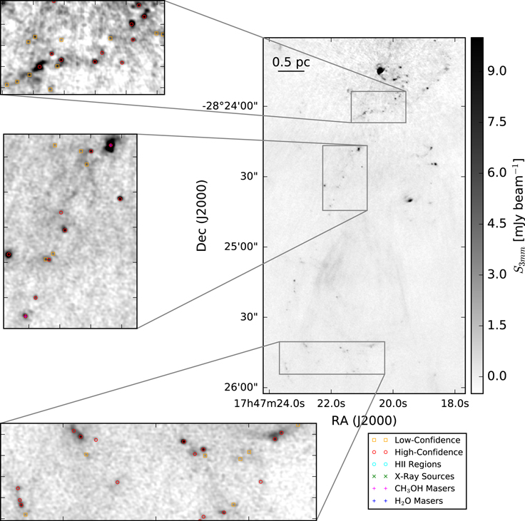
Figure 5. Close-in look at the Sgr B2 DS region. Multiple insets show identified sources in some of the richer subregions. The points are colored as in Figure 2. The background image is the ALMA 3 mm continuum.
Download figure:
Standard image High-resolution imageOutside of the dense clusters, every peak that is higher than five times the lowest measured rms noise value was visually inspected. Peaks that were part of extended structures but not significantly different from them (e.g., a 5σ peak sitting on a 4σ extended structure) were excluded. We excluded sources with radial extents  (
( pc), i.e., extended H ii regions (all such sources have corresponding centimeter-wavelength detections indicating that they are H ii regions).
We measure the local noise for each source by computing the median absolute deviation in an annulus 05–1
5 around the source center; these noise measurements are reported in Appendix C in Table 3.
Our selection criteria result in a reliable but potentially incomplete catalog; because we did not employ an automated source identification algorithm, we cannot readily quantify our completeness. The regions most likely to be incomplete near our noise threshold are Sgr B2 M and N. In these regions, dynamic range limitations increase the background noise and make fainter sources difficult to detect, as described in Section 2. Additionally, they both contain extended structures, including H ii regions and dust filaments, which likely obscure compact sources.
For a subset of the sources, primarily the brightest, we measured the spectral index α based on CASA tclean's two-term Taylor expansion model of the data (parameters deconvolver = ‘‘mtmfs’’ and nterms = 2). This measurement is over a narrow frequency range (≈90–100 GHz). tclean produces α and  (error on α) maps, and we used the α value at the position of peak intensity for each source. We include in the analysis only those sources with
  or
or  the latter include sources with
  measured at relatively high precision. We exclude the lower-precision measurements of α because they are not useful for identifying the emission mechanism. Of the 271 detected sources, 62 met these criteria. Several of the brightest sources did not have significant measurements of α because they are in the immediate neighborhood of Sgr B2 M or N and therefore have significantly higher background and noise, preventing a clear measurement.
To check the calibration of the spectral index measurement, we imaged one of our calibrators, J1752–2956, and obtained a spectral index  , consistent with the expected
  for an optically thin synchrotron source (e.g., Condon & Ransom 2007). We also note that the relative spectral index measurements in our catalog should be accurate, since all sources come from the same map with identical calibration.
We detected 271 compact continuum sources, and they are listed in Table 3. Their flux distribution is shown in Figure 6. The distribution of their measured spectral indices α is shown in Figure 7. Generally, spectral indices  indicate nonthermal (e.g., synchrotron) emission,
  may correspond to free–free sources of various optical depths,
  for any optically thick thermal source, and
  usually indicates optically thin dust emission. These indices will be discussed further in Section 3.3.
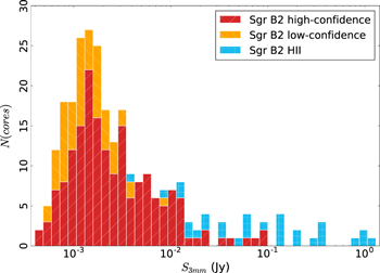
Figure 6. Histogram of the flux density (the peak intensity converted to flux density assuming that the source is unresolved) of the observed sources. The histograms are stacked such that there are a total of 27 sources in the highest bin.
Download figure:
Standard image High-resolution image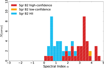
Figure 7. Histogram of the spectral index α for those sources with a statistically significant measurement. The H ii regions cluster around  , as expected for optically thin free–free emission, while the unclassified sources cluster around
  , which is consistent with dust emission.
Download figure:
Standard image High-resolution image3.2. Source Classification Based on Catalog Cross-matching
We cross-matched our source catalog with catalogs of  sources, H ii regions, X-ray sources, Spitzer sources, and methanol and water masers.
H ii regions—We classified sources as H ii regions if there is a corresponding 0.7 or 1.3 cm source from one of the previous VLA surveys (Gaume et al. 1995; Mehringer et al. 1995; De Pree et al. 1996, 2015) within one ALMA beam (05). A total of 31 of our sources are classified as H ii regions; these all have
 mJy. The majority of these are unresolved, but we have included H ii regions with radii up to
  in our catalog. Optically thick H ii regions (like any blackbody) have a spectral index
  . Optically thin H ii regions have a nearly flat spectral index,
  (Condon & Ransom 2007). The observed sources with H ii region counterparts have spectral indices consistent with the theoretical expectation for optically thin H ii regions in Figure 7. The existing VLA data do not cover the entire area of our observations, so we only have a lower limit on the number of H ii regions in our sample; the sources in Sgr B2 DS have not yet been observed in the radio at high resolution. Sources matched with H ii regions evidently contain high-mass (most likely
  ; see Section 3.3.4 below) young stars.
 sources—Martín-Pintado et al. (1999) observed part of Sgr B2 DS and M in
  with the VLA. They identified three “hot cores” based on
  (4, 4) detections. Only their first source HC1 has an associated 3 mm continuum source, suggesting that HC2 and HC3 are not genuine hot cores but are some other variant of locally heated (perhaps shock-heated) gas. However, the association between HC1 and our source 43 suggests that it is a YSO with a massive envelope. Of the six
  (3, 3) maser sources identified by Martín-Pintado et al. (1999), three are in regions with high 3 mm source density but lack a clear one-to-one source association, one is coincident with an extended H ii region not in our catalog, and two have no obvious associations. The
  (3, 3) masers therefore do not appear to be unambiguous tracers of star formation in this environment, consistent with the conclusions of Mills et al. (2015).
6.67 GHz  masers—Class II methanol masers are exclusively associated with sites of high-mass star formation. The Caswell et al. (2010) Methanol Multibeam (MMB) Survey identified 11 sources in our observed field of view (their survey covers our entire observed area), of which 10 have a clear match to within 1″ of a source in our catalog (the MMB catalog sources have a positional accuracy of
  , but masers may have an extent up to 1″). These sources are clearly identified as high-mass YSOs. The single maser that does not have an associated millimeter source is 5″ west of Sgr B2 S and resides near some very faint and diffuse 3 mm emission; it is unclear why the 3 mm is so weak here, but it hints that there are high-mass YSOs with 3 mm emission below our detection limit.
H2O masers—Water masers are generally associated with young, accreting stars. We matched our catalog with the McGrath et al. (2004) water maser catalog, finding that 23 of our sources have a water maser within 1″. These sources are likely to contain YSOs, but not necessarily high-mass YSOs based on their H2O maser detections alone. There are 14 masers from their catalog that do not have associated sources in our catalog, though not all of these maser spots are spatially distinct. Most of these unassociated masers are seen outside of Sgr B2 N and Sgr B2 S and may be associated with outflows. This catalog covers about 10% of our mapped area with their single VLA K-band pointing; their map excludes the many sources in Sgr B2 DS.
X-ray sources—Some young stars exhibit X-ray emission, including some high-mass YSOs (e.g., Townsley et al. 2014), so we searched for X-ray emission from our sources. Three of the sources have X-ray counterparts in the Muno et al. (2009) Chandra point-source catalog within 1″. The Muno et al. (2009) catalog covers our entire observed area. The X-ray-associated sources most likely contain YSOs. There are 102 X-ray sources in the field of view that do not have associated 3 mm sources.
Spitzer mid-infrared sources—We searched the Yusef-Zadeh et al. (2009) catalogs of 4.5  excess sources and YSO candidates and found only one source association, though there are 5 and 14, respectively, of these sources in our field of view. Two of the 4.5
  excess sources and one of the YSO candidates are associated with extended H ii regions (which we do not catalog); the single association is of a 4.5
  source with the central region of Sgr B2 M. By-eye comparison of the Spitzer maps and the ALMA images suggests that the lack of associations is at least in part because of the high extinction in the regions containing the 3 mm cores; there are overall fewer Spitzer sources in these parts of the maps.
44 GHz  masers—Finally, we searched the Mehringer & Menten (1997) sample of 44 GHz Class I
  maser sources for associations, finding no matches with any of our sources out of the 18 nonthermal
  emission sources they reported. This methanol maser line apparently does not trace star formation. Their maps include two VLA Q-band images pointed at Sgr B2 M and N; these maps cover only a very small fraction (∼5%) of our mapped area.
3.3. Nature of the Continuum Sources
The majority of the detected sources are observed only as 3 mm continuum sources, with no spectral line information or detection at other wavelengths. In this section, we employ a variety of arguments to classify the sample of new sources. Plausible emission mechanisms include free–free and thermal dust emission, so in this section we explore whether the sources could be different classes of dust or free–free sources. We examine whether they are prestellar cores (Section 3.3.1), externally ionized globules (Section 3.3.2), H ii regions from an extended population of OB stars (Section 3.3.3), or H ii regions around young massive stars (Section 3.3.4). After determining that the above alternatives do not readily explain the whole sample, we conclude that the sources are primarily dense gas and dust cores with internal heating sources (Section 3.3.5).
A lack of line emission—We visually inspected the spectra extracted from the full line cubes, and no lines are detected peaking toward most of the sources (most sources have emission in some lines, such as  10–9, but this emission is clearly extended and not associated with the compact source). Given the relatively poor line sensitivity (rms ≈ 6 K), the dearth of detections is not very surprising. We therefore cannot use spectral lines to classify most sources.
3.3.1. Alternative 1: The Sources Are “Prestellar” Cores
The simplest assumption is that all sources we have detected that were not detected at longer wavelengths are pure dust emission sources at a constant temperature, i.e., they are starless cores.
At  , a 1 mJy source corresponds to an optically thin gas mass26
of
, a 1 mJy source corresponds to an optically thin gas mass26
of  or
or  assuming a dust opacity index
  (spectral index
  if measured on the Rayleigh–Jeans tail of the SED) to extrapolate the Ossenkopf & Henning (1994, MRN with thin ice mantles anchored at 1 mm) opacity to
  cm2 g−1 (per gram of gas). Our dust-only (i.e., excluding free–free emission) 5σ sensitivity limit at 20 K therefore ranges from
  (0.5 mJy) to
  (2.5 mJy) across the map. If we were to assume that these are all cold, dusty sources, as is typically (and reasonably) assumed for local clouds, they would be extremely massive and dense, with the lowest measurable density being
  (corresponding to 19
  in an
in an  radius sphere, i.e., a sphere with radius equal to the beam 1σ size).
Such extreme objects are technically possible, but we argue that the majority are unlikely to fall into this class. We have detected  of these sources, but only a handful of comparable-mass starless cores have ever been claimed before (e.g., Kong et al. 2017), and few of those reported are so compact (e.g., Cyganowski et al. 2014). Theoretical models of high-mass prestellar cores (McKee & Tan 2003) suggest that they are much larger and less concentrated than the sources we observe.
At the high implied densities ( ), it is unlikely that the cores are unbound; these sources have
  from
from  . The high density required for our sources results in a short free-fall timescale,
  . Assuming that such cores do exist, the timescale for them to form a central YSO (a central heating source) is short. While there are few constraints on the accreting lifetime of high-mass YSOs, that timescale is almost certainly 1–2 orders of magnitude longer. For a given population of cores, we would expect only of order 1%–10% of them to be starless at any given time. We will revisit the characteristics of centrally heated dust sources in Section 3.3.5 below.
3.3.2. Alternative 2: The Sources Are Externally Ionized Gas Blobs
One possibility is that these sources are not dust dominated, nor pre- or protostellar, but are instead externally ionized, mostly neutral gas clumps embedded within diffuse H ii regions. They would then be analogous to the heads of cometary clouds, externally ionized globules (“EGGs”; Sahai et al. 2012a), or proplyds (externally ionized protoplanetary disks), and their observed emission would give little clue to their nature because the light source is extrinsic.
The majority of the detected sources have size  , i.e., they are unresolved.27
By contrast, the free-floating EGGs (“frEGGs”) so far observed have sizes 10,000–20,000 au (Sahai et al. 2012a, 2012b), so they would be resolved in our observations. Toward the brightest frEGG in Cygnus X, Sahai et al. (2012b) measured a peak intensity
, i.e., they are unresolved.27
By contrast, the free-floating EGGs (“frEGGs”) so far observed have sizes 10,000–20,000 au (Sahai et al. 2012a, 2012b), so they would be resolved in our observations. Toward the brightest frEGG in Cygnus X, Sahai et al. (2012b) measured a peak intensity  mJy beam−1 in a
  beam. Cygnus X is
  closer than the Galactic center, so their beam size is the same physical scale as ours. If the free–free emission is thin (
 ), the brightness in our data would be
  mJy beam−1. These frEGGs would be detectable in our data. Comparison to radio observations at a similar resolution will be needed to rule out the externally ionized globule hypothesis for the resolved regions within our sample. However, the unresolved sources in our sample are unlikely to be frEGGs, since they are too small.
If the detected sources were either EGGs or cometary clouds, we would expect them to be located within diffuse H ii regions, since that is where all other sources of this type are seen, and since an external ionizing agent is needed to illuminate them. Many of the sources are near, but not embedded in, H ii regions, as seen in Figure 8(a), which shows 20 cm continuum emission that most likely traces ionized gas. The sources are nearly all associated with a ridge of molecular ( ) emission (Figure 8(b)). If they are deeply embedded within the molecular material, they cannot be externally ionized.
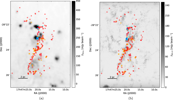
Figure 8. Left: location of the detected continuum sources (red circles) overlaid on a 20 cm continuum VLA map highlighting the diffuse free–free (or possibly synchrotron) emission in the region (Yusef-Zadeh et al. 2004). Right: continuum sources overlaid on a map of the  J = 10–9 peak intensity over the range [−200, 200]
  . In both panels, red circles are “conservative,” high-confidence sources; orange squares are “optimistic,” low-confidence sources; cyan circles are H ii regions; magenta plus signs are
  masers; blue plus signs are H2O masers; and green crosses are X-ray sources.
Download figure:
Standard image High-resolution imageThe ionized gas emission (20 cm, Figure 8(a)) and molecular gas emission ( , Figure 8(b)) are anticorrelated. The
  emission wraps around the 20 cm emission and has a significant extent beyond the edge of the 20 cm emission. If the
  were tracing a photon-dominated region, we would expect the
  emission to peak along the edge of the H ii region. Since it does not, we conclude that the
  emission is tracing a “quiescent” molecular cloud, i.e., one that is not significantly heated by the adjacent H ii region. Most of the 3 mm sources are aligned with bright
  emission, implying that they are embedded within it. If they are indeed embedded in an extended molecular cloud, that cloud should shield them from ionizing radiation. The sources are therefore mostly not externally ionized.
A final point against the externally ionized hypothesis is the observed spectral indices shown in Figure 7. We measured spectral indices for 62 sources, of which 33 have  . These 33 sources are inconsistent with free–free emission and are at least reasonably consistent with dust emission.
3.3.3. Alternative 3: The Sources Are H ii Regions Produced by Interloper Ionizing Stars
If there is a large population of older (age 1–30 Myr) massive stars, they could ignite compact H ii regions when they fly through molecular material. In other words, each OB star that encounters dense enough gas would create a compact H ii region that would not have time to expand owing to the star’s rapid motion. Such sources would be bow shaped when viewed at higher resolution. See Section 3.3.4 for calculations of stationary H ii region properties.
The main problem with this scenario is the spatial distribution of the observed sources. While most of the continuum sources are associated with dense gas and dust ridges, not all of the high column density molecular gas regions have such sources in them (see Figure 8(b), where there is some molecular material that does not have associated millimeter sources, especially to the east and west of the main ridge). If there is a free-floating population of OB stars responsible for the 3 mm compact source population, and if we assume that the spatial distribution of the stars is uniform, the distribution of the resulting H ii regions should match that of the gas. Also, there is no such population of sources seen outside of the dense gas in the infrared, which again we should expect if there is a uniformly distributed massive stellar population. Finally, the spectral indices discussed above (Figure 7) suggest that the previously unidentified sources are dust emission sources, not free–free sources.
3.3.4. Alternative 4: The Sources Are H ii Regions Produced by Recently Formed OB Stars
We know from previous observations (e.g., Mehringer et al. 1995; De Pree et al. 1996, 2015) that there is a substantial population of H ii regions in the Sgr B2 clusters. The 31 sources associated with these previously identified H ii regions are among the brightest in our catalog. We address here whether the remaining sources, which are mostly fainter, could also be H ii regions.
To calculate the expected 3 mm flux density from an H ii region with a central source emitting Lyman continuum luminosity Qlyc, we rearrange Condon & Ransom’s (2007) Equations (4.60) and (4.61). We get an equation for the expected brightness temperature as a function of electron temperature Te, emission measure EM, and frequency ν:


where Qlyc is the count rate of ionizing photons in  , τ is the optical depth of the H ii region,
  is the case B recombination coefficient, and R is the H ii region radius. The emission measure EM* assumes that the H ii region is a uniform-density Strömgren sphere. The constant c* was computed by Mezger & Henderson (1967) as an approximation to the optical depth prefactor in the full radiative transfer equation and is never incorrect by more than
  . To convert the above brightness temperature into a flux density, assuming an
  beam at 95 GHz,
  .
.
For an unresolved spherically symmetric H ii region ( ), the expected flux density is
  for a
for a  source (assuming
  ), and that value scales linearly with Qlyc as long as the source is optically thin (in the optically thin
  limit, Equation 1(a) becomes approximately
  ).
).
An extremely compact H ii region, e.g., one with  and corresponding density
  , would be somewhat optically thick (
 ) and therefore fainter,
  . Even the most luminous O stars could produce H ii regions as faint as 0.5 mJy if embedded in extremely high density gas; above
  , a 25 au H ii region would have
  mJy (
mJy ( ).
).
Figure 9 shows the predicted brightness for various H ii regions produced by OB stars and the density required for those H ii regions to be the specified size. There is a narrow range of late O/early B28
stars,  , that could be embedded in compact H ii regions of almost any size and produce the observed range of flux densities. In order for the detected sources to be O-star-driven H ii regions, with
  , they must be optically thick and therefore extremely compact and dense. Anything fainter, i.e., later than ∼B2 (
 ), would be incapable of producing the observed flux densities.
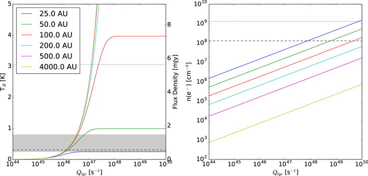
Figure 9. Simple models of spherical H ii regions to illustrate the observable properties of such regions. The H ii region size is shown by line color; the legend in the left panel applies to both figures. Left: expected brightness temperature (left axis) and corresponding flux density at 95 GHz within an FWHM = 05 beam (right axis) as a function of the Lyman continuum luminosity for a variety of source radii. The gray filled region shows the range of our 5σ sensitivity limits, which vary with location from 0.25 to 0.8 K. The dotted and dashed horizontal lines show the flux density of a 10 and 100
 isothermal dust core at T = 40 K. Right: electron density required to produce an H ii region of radius indicated by the legend in the left panel. The horizontal dashed line shows the density corresponding to an unresolved dust source (
 au) at the 5σ detection limit (
 mJy, or 10
  of dust, assuming T = 40 K, and assuming
  ). The dotted line shows the density corresponding to a 100
  dust core at T = 40 K.
Download figure:
Standard image High-resolution imageThe 119 sources with  mJy that were not previously identified as H ii regions from radio data require a finely tuned set of parameters to be H ii regions. Stars emitting
  photons s–1 (B1.5–B2 main-sequence stars, with
  ) could reside in H ii regions spanning a wide range of radii and produce flux densities in the observed range (Figure 9(a)). More luminous stars could reside in 50–100 au H ii regions and produce the observed flux densities, but such small regions are expected to be very short-lived and therefore rare. It is unlikely that nearly half of the stars are between 8 and 10
  , since such a local mass peak would imply a highly abnormal initial mass function (IMF).29
We therefore assume that the newly detected sources are not predominantly H ii regions.
, since such a local mass peak would imply a highly abnormal initial mass function (IMF).29
We therefore assume that the newly detected sources are not predominantly H ii regions.
For completeness, we assess the emission properties of the dust surrounding hypercompact H ii regions, since, in order to remain hypercompact, the stars must be surrounded by very dense gas. Figure 9(b) shows that if O stars were confined to H ii regions small enough to produce the median source flux density (2 mJy), the emission could be dominated by a surrounding warm (40 K) dust core. Such sources would be at least twice as bright as predicted in Figure 9(a). Only the most luminous O stars are affected by this consideration; however, this panel also illustrates that O stars will almost certainly be detected in our data no matter how dense their surroundings.
A final point against the sample being exclusively H ii regions is the observed spectral indices. While some are consistent with H ii regions, with  , some (
 ) are steeper than
  and are therefore inconsistent with free–free emission.
3.3.5. Alternative 5, Our Hypothesis: The Sources Are (Mostly) YSOs
After determining that the other possibilities cannot explain the whole sample, we test and validate the hypothesis that most or all of the sources contain YSOs in this section.
If we assume that the sources are dust dominated and have a higher dust temperature than used in Section 3.3.1, the inferred gas mass is lower, but an internal heating source—i.e., a protostar or young star—is required. For example, if we assume TD = 80 K,30
our detection limit is only  . Heating that much dust well above the cloud average requires a high-luminosity central heating source.
To constrain the required heating source, we examine the protostellar models of Robitaille (2017, specifically, the spubhmi and spubsmi models) and Zhang & Tan (2015). The Robitaille models that produce  mJy within an
  aperture uniformly have
  . Such luminosities imply either that a high-mass (
 ) star has already formed and is still surrounded by a massive envelope or that a high-mass YSO is present and accreting. The models of Zhang & Tan (2015) generally only exhibit
  once a star has reached
  as it continues to accrete to a higher mass. Similarly, pre-main-sequence stellar evolution models (e.g., Haemmerlé et al. 2013) only reach
  at any point in their evolution for stars with final mass
  . In the Robitaille (2017) model grid, all sources with
  produce
  mJy, so our survey should be nearly complete to such sources, but in the range
  , a substantial fraction may be below our sensitivity limit.
Comparison to similar data—We compare our detected sample to that of the Herschel Orion Protostar Survey (HOPS; Furlan et al. 2016) in order to get a general empirical sense of what types of sources we have detected. We selected this survey for comparison because it is one of the largest protostellar core samples with well-characterized bolometric luminosities available. Figure 10 shows the HOPS source flux densities at 870  (from LABOCA on the APEX telescope) scaled to
  and 3 mm assuming a dust opacity index
  , which is shallower than usually inferred, so the extrapolated fluxes may be slightly overestimated.31
The 870
, which is shallower than usually inferred, so the extrapolated fluxes may be slightly overestimated.31
The 870  data were acquired with a
  , which translates to a resolution of ∼1″ at
  assuming
  pc, so our beam size is somewhat smaller than theirs.
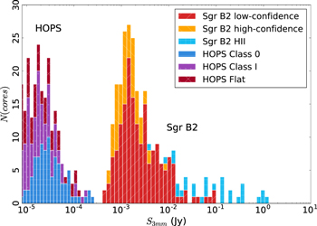
Figure 10. Histogram combining the detected Sgr B2 cores with predicted flux densities for sources at  and
and  based on the HOPS (Furlan et al. 2016) survey. The sources are labeled by their infrared (2–20
  ) spectral index: Classes 0 and I have positive spectral index, and flat-spectrum sources have
  . The HOPS histogram shows the 870
  data from that survey scaled to 3 mm assuming
  (see footnote 31). Every HOPS source is well below the detection threshold for our observations.
Download figure:
Standard image High-resolution imageThe HOPS sources are all fainter than even the faintest Sgr B2 sources. The most luminous and brightest HOPS source, with  , would only be 0.2 mJy in Sgr B2, or about a 2σ source, which is below our detection threshold even in the artifact-free regions of the map. We conclude that the Sgr B2 sources are much more luminous than any in the Orion sample, which is consistent with all of the sources in our sample being high-mass YSOs.
This conclusion is supported by a more direct comparison with the Orion Nebula as observed at 3 mm with MUSTANG (Dicker et al. 2009; Figure 11). Their data were taken at 9″ FWHM resolution, corresponding to 048 at
 . The peak flux density measured in that map is toward Source I,
  mJy. Source I32
would therefore be detected and would be somewhere in the middle of our sample. It resides on a background of extended emission, and the extended component would be readily detected (and resolved) in our data. Source I is the only known high-mass YSO in the Orion cloud, and it would be detectable in our survey, while no other compact sources in the Orion cloud would be. This comparison supports the interpretation that most of the non-H ii region sources are massive YSOs.
mJy. Source I32
would therefore be detected and would be somewhere in the middle of our sample. It resides on a background of extended emission, and the extended component would be readily detected (and resolved) in our data. Source I is the only known high-mass YSO in the Orion cloud, and it would be detectable in our survey, while no other compact sources in the Orion cloud would be. This comparison supports the interpretation that most of the non-H ii region sources are massive YSOs.
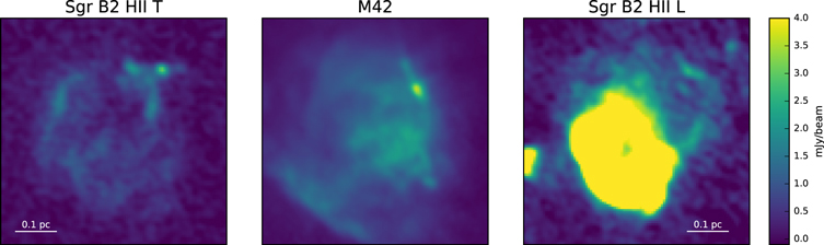
Figure 11. Comparison of two extended H ii regions in Sgr B2 (ALMA 3 mm continuum) to the M42 (GBT MUSTANG 3 mm continuum; Dicker et al. 2009) nebula in Orion. The three panels are shown on the same physical and color scale assuming  pc and
  and that the ALMA and MUSTANG data have the same continuum bandpass. Sgr B2 H ii T is comparable in brightness and extent to M42; Sgr B2 H ii L is much brighter and is saturated on the displayed brightness scale. The compact source to the top right of the M42 image is Orion Source I; the images demonstrate that Source I and the entire M42 nebula would be easily detected in our data.
Download figure:
Standard image High-resolution imageThe spectral indices of the dusty sources—While we have concluded that the sources are dusty, massive YSOs, the spectral indices we measured are somewhat surprising. Typical dust clouds in the Galactic disk have dust opacity indices  , implying a spectral index
  (
( Schnee et al. 2010; Shirley et al. 2011; Sadavoy et al. 2016). Our spectral index measurements are lower than these: only 3 sources out of 62 with significant α measurements have
  ,33
though 33 of the sources with α measurements have
,33
though 33 of the sources with α measurements have  , indicating that their emission is dust dominated. A shallower β implies that free–free contamination, large dust grains, or optically thick surfaces are present within our sources. Since the arguments in previous sections suggest that the sources are high-mass YSOs, the free–free contamination and optically thick inner region models are both plausible.
4. Analysis and Discussion of Star Formation in Sgr B2
We have reported the detection of a large number of point sources and inferred that they are most likely all high-mass YSOs. In this section, we discuss the source flux density distribution function and SFR estimates (Section 4.1), the difference between the clustered and distributed source populations (Section 4.2), star formation surface density thresholds (Section 4.3), star formation and gas surface density relations (Section 4.4), and the implications of a varying volume density threshold (Section 4.5).
4.1. Source Distribution Functions and the Star Formation Rate
In this section we examine the distribution of observed flux densities and the implied total stellar masses.
If we make the very simplistic, but justified (Section 3.3.5), assumption that the sources we detect all contain YSOs with 
 , and in turn make the related assumption that each source either currently contains or will form into an
  star, we can infer the total (proto)stellar mass in the observed region.
We assume the stellar masses based on the arguments in Section 3.3.5: in order to be detected, the sources must be either active OB stars illuminating H ii regions, very compact cores with  of warm dust within
  , or at least moderately massive YSOs within warm envelopes. Note that the mass estimates in this section are for the resulting stars, not their envelopes.
To compute the total mass of the forming star populations, we assume that each source not associated with an H ii region contains or will form a star with mass equal to the average over the range 8–20  assuming a Kroupa (2001, Equation (2)) IMF,
  (in this section, we refer to these objects as “cores”). Based on the arguments in Section 3.3.4, we assume that each H ii region contains a star that is B0 or earlier, and therefore that they each have a mass equal to the average over 20
  ,
,  . In Table 2, the total counted mass estimate is shown as
  , where N is the number of stars with an assumed mass
  .
.
Table 2. Cluster Masses
| Name | N(cores) |

|
Mcount | Minferred |

|

|
Mcounts | Minfs | SFR |
|---|---|---|---|---|---|---|---|---|---|
( ) ) |
( ) ) |
( ) ) |
( ) ) |
( ) ) |
( ) ) |
( ) ) |
|||
| M | 17 | 47 | 2300 | 8800 | 15000 | 2300 | 1295 | 20700 | 0.012 |
| N | 11 | 3 | 270 | 1200 | 980 | 1500 | 150 | 2400 | 0.0017 |
| NE | 4 | 0 | 48 | 270 | 0 | 540 | 52 | 1200 | 0.00037 |
| S | 5 | 1 | 110 | 500 | 330 | 680 | 50 | 1100 | 0.00068 |
| Unassociated | 203 | 6 | 2700 | 15000 | 2000 | 27000 | ⋯ | ⋯ | 0.02 |
| Total | 240 | 57 | 5500 | 26000 | 19000 | 33000 | 1993 | 33400 | 0.035 |
| Totalmax | ⋯ | ⋯ | ⋯ | 46000 | ⋯ | ⋯ | ⋯ | ⋯ | 0.062 |
Note. Mcount is the mass of directly counted protostars, assuming that each millimeter source is 12.0  , or 45.5
  if it is also an H ii region.
  and
and  are the inferred total stellar masses assuming that the counted objects represent fractions of the total mass 0.09 (cores) and 0.14 (H ii regions). Minferred is the average of these two. Mcounts and Minfs are the counted and inferred masses reported in Schmiedeke et al. (2016). The SFR is computed using Minferred and an age
  , which is the time of the last pericenter passage in the Kruijssen et al. (2015) model. The Total row represents the total over the whole observed region. The Totalmax row takes the higher of
  and
and  from each row and sums them. We have included H ii regions in the N(H ii) counts that are not included in our source Table 3 because they are too diffuse, or because they are unresolved in our data but were resolved in the De Pree et al. (2014) VLA data. As a result, the total source count is greater than the source count reported in Table 3. Also, the unassociated H ii region count is incomplete; it is missing both diffuse H ii regions and possibly unresolved hypercompact H ii regions, since there are no VLA observations comparable to De Pree et al. (2014) in the unassociated regions.
Download table as: ASCIITypeset image
We also compute the total stellar mass (i.e., the extrapolated mass including low-mass stars) using the mass fractions  and
and  derived from the assumed IMF. The total mass inferred by extrapolating our measurements with this IMF is then


The inferred masses computed from H ii region counts and from core counts are shown in columns  and
and  of Table 2, respectively. Minferred is the average of these two estimates; it is also what would be obtained if all stars were assumed to be average stars with
  . If our mass range classifications are correct and the mass distribution is governed by a power-law IMF, we expect
  .
.
We identify each source as belonging to one of the clusters described in Schmiedeke et al. (2016; the clusters are labeled in Figure 1). In each cluster, we count the number of H ii regions identified in our survey plus those identified in previous works (Gaume et al. 1995; De Pree et al. 1996), and we count the number of protostellar cores not associated with H ii regions. The distributions of source flux densities associated with each cluster are shown in Figure 12. The cluster affiliation for each source is reported in Table 3.
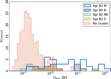
Figure 12. Histograms showing the flux density (the peak intensity converted to flux density assuming that the source is unresolved) of the observed sources classified by their cluster association. Unlike Figure 6, the histograms are overlapping, not stacked. The bin widths for the clusters are wider than for the unassociated sources.
Download figure:
Standard image High-resolution imageTable 3. Continuum Source IDs and Photometry
| ID | Cluster | Classification |

|

|

|

|
α |

|
M40 K |

|
Coordinates |
|---|---|---|---|---|---|---|---|---|---|---|---|
| 174 f3 | M | S__W HII | 1600 | 860 | 2400 | 46 | 0.89 | 0.002 | ⋯ | ⋯ | 17:47:20.167, –28:23:04.809 |
| 234 f4 | M | S__W HII | 1100 | 570 | 900 | 23 | 0.83 | 0.001 | ⋯ | ⋯ | 17:47:20.214, –28:23:04.379 |
| 176 f1 | M | S__W HII | 920 | 480 | 1400 | 30 | 1.2 | 0.006 | ⋯ | ⋯ | 17:47:20.127, –28:23:04.082 |
| 236 f10.303 | M | S__W HII | 880 | 460 | 800 | 20 | 1.1 | 0.015 | ⋯ | ⋯ | 17:47:20.106, –28:23:03.729 |
| 235 f2 | M | S__W HII | 820 | 430 | 670 | 33 | 1.3 | 0.002 | ⋯ | ⋯ | 17:47:20.166, –28:23:03.714 |
| 172 K2 | N | S__W HII | 370 | 200 | 650 | 49 | 2.5 | 0.018 | ⋯ | ⋯ | 17:47:19.869, –28:22:18.466 |
| 265 H | S | S__W HII | 360 | 190 | 580 | 3.9 | 0.65 | 0.019 | ⋯ | ⋯ | 17:47:20.461, –28:23:45.404 |
| 175 G | M | S__W HII | 340 | 180 | 390 | 5.6 | 0.68 | 0.03 | ⋯ | ⋯ | 17:47:20.285, –28:23:03.162 |
| 237 G10.44 | M | S__W HII | 280 | 140 | 160 | 15 | 0.69 | 0.006 | ⋯ | ⋯ | 17:47:20.241, –28:23:03.387 |
| 178 f10.37 | M | SX_W HII | 200 | 100 | 270 | 18 | 1.5 | 0.039 | ⋯ | ⋯ | 17:47:20.178, –28:23:06 |
| 171 K3 | N | S__W HII | 180 | 97 | 280 | 25 | 1.4 | 0.023 | ⋯ | ⋯ | 17:47:19.895, –28:22:17.221 |
| 177 B | M | S___ HII | 150 | 77 | 240 | 3.9 | 0.47 | 0.011 | ⋯ | ⋯ | 17:47:19.918, –28:23:03.039 |
| 241 f10.30 | M | S__W HII | 140 | 73 | 120 | 15 | 1.4 | 0.05 | ⋯ | ⋯ | 17:47:20.106, –28:23:03.066 |
| 179 f10.38 | M | S__W HII | 130 | 66 | 180 | 9.3 | 1.6 | 0.013 | ⋯ | ⋯ | 17:47:20.193, –28:23:06.673 |
| 180 E | M | S___ HII | 130 | 66 | 190 | 4 | 0.38 | 0.014 | ⋯ | ⋯ | 17:47:20.108, –28:23:08.894 |
| 173 K1 | N | S___ HII | 92 | 48 | 150 | 4.4 | 0.58 | 0.034 | ⋯ | ⋯ | 17:47:19.78, –28:22:20.743 |
| 170 | N | S__W PartofCloud | 92 | 48 | 160 | 22 | 1.7 | 0.082 | ⋯ | ⋯ | 17:47:19.895, –28:22:13.621 |
| 252 | N | S__W denseCore | 82 | 43 | 160 | 16 | 1.9 | 0.078 | ⋯ | ⋯ | 17:47:19.862, –28:22:13.168 |
| 225 f10.33b | M | SX_W denseCore | 69 | 36 | 100 | 14 | 1.9 | 0.21 | 1200 | 3.6 × 1026 | 17:47:20.116, –28:23:06.374 |
| 264 k4 | ⋯ | S___ HII | 65 | 34 | 140 | 3.5 | 0.57 | 0.034 | 1100 | 2.6 × 1026 | 17:47:19.997, –28:22:04.648 |
| 96 Z10.24 | ⋯ | S_MW Maser | 64 | 33 | 75 | 1.5 | 0.68 | 0.37 | 1100 | 2.5 × 1026 | 17:47:20.039, –28:22:41.25 |
| 181 D | M | S_M_ HII | 59 | 31 | 94 | 1.3 | 0.64 | 0.088 | 1000 | 2 × 1026 | 17:47:20.051, –28:23:12.91 |
| 240 f10.44b | M | S__W HII | 57 | 30 | 51 | 11 | 1.8 | 0.016 | 960 | 1.8 × 1026 | 17:47:20.252, –28:23:06.463 |
| 233 f10.27b | M | S__W HII | 50 | 26 | 78 | 18 | 2.3 | 0.18 | 840 | 1.4 × 1026 | 17:47:20.077, –28:23:05.383 |
| 239 | M | S__W denseCore | 45 | 24 | 46 | 8.6 | 2.3 | 0.091 | 760 | 1.1 × 1026 | 17:47:20.242, –28:23:07.222 |
| 244 C | M | S___ ⋯ | 36 | 19 | 67 | 0.49 | 0.47 | 0.081 | 600 | 7.8 × 1025 | 17:47:19.981, –28:23:18.437 |
| 242 f10.318 | M | S__W HII | 32 | 17 | 63 | 8.5 | 2.2 | 0.099 | 540 | 6.8 × 1025 | 17:47:20.129, –28:23:02.247 |
| 92 I10.52 | M | S___ HII | 32 | 17 | 45 | 5.3 | 0.63 | 0.061 | 530 | 6.6 × 1025 | 17:47:20.324, –28:23:08.2 |
| 245 A2 | ⋯ | S___ HII | 24 | 13 | 32 | 2.1 | 0.54 | 0.025 | 410 | 4.8 × 1025 | 17:47:19.562, –28:22:55.916 |
| 109 | N | S__W ⋯ | 24 | 13 | 41 | 13 | 3.6 | 0.3 | 410 | 4.7 × 1025 | 17:47:19.901, –28:22:15.54 |
| 87 B9.99 | M | S___ HII | 23 | 12 | 37 | 1.9 | 0.89 | 0.042 | 390 | 4.4 × 1025 | 17:47:19.798, –28:23:06.942 |
| 88 | M | S__W ⋯ | 23 | 12 | 34 | 2.9 | 3.1 | 0.18 | 380 | 4.3 × 1025 | 17:47:19.617, –28:23:08.26 |
| 151 B10.06 | M | S_M_ HII | 20 | 11 | 31 | 1.3 | 0.19 | 0.79 | 350 | 3.8 × 1025 | 17:47:19.86, –28:23:01.5 |
| 98 | ⋯ | S_M_ Maser | 18 | 9.5 | 29 | 0.36 | 3.2 | 1.1 | 300 | 3.3 × 1025 | 17:47:19.53, –28:22:32.55 |
Note. The Classification column consists of three-letter codes as described in Section 3.3. In column 1, S indicates a strong source, and W indicates a weak or low-confidence source. In column 2, an X indicates a match with the Muno et al. (2009) Chandra X-ray source catalog, while an underscore indicates that there was no match. In column 3, M indicates a match with the Caswell et al. (2010) Methanol Multibeam Survey  maser catalog, while an underscore indicates that there was no match. Finally, we include the SIMBAD (Wenger et al. 2000) source object type classification if one was found. The full electronic version of this table is available at https://github.com/keflavich/SgrB2_ALMA_3mm_Mosaic/blob/master/tables/continuum_photometry_withSIMBAD_andclusters.ipac and will be made available via the journal at the time of publication.
Only a portion of this table is shown here to demonstrate its form and content. A machine-readable version of the full table is available.
Download table as: DataTypeset image
In Sgr B2 N and S, the core-based and H ii-region-based estimates agree to within a factor of 2, which is about as good as expected from Poisson noise in the counting statistics. Sgr B2 M contains the largest source sample, and it has a factor of nine discrepancy between the core- and H ii-region-based counts. The discrepancy may arise from the combined effects of source confusion at our 05 resolution and the increased noise around the extremely bright central region that makes detection of
 mJy sources difficult. The majority of pixels within the cluster region have significant detections at 3 mm, but we do not currently have the capability to distinguish between extended dust emission, free–free emission, or a confusion-limited point-source population. While it is possible that this discrepancy is driven by observational limitations, we also explore in Section 4.2 the possibility that it is a real physical effect.
We compare our mass estimates with those of Schmiedeke et al. (2016), who inferred stellar masses from H ii region counts. The two columns of Table 2 with superscript S show their observed and estimated masses based on H ii region counts. For Sgr B2 M and N, our results are similar, as expected since our catalogs are similar. For S and NE, we differ by a large factor, primarily because Schmiedeke et al. (2016) assumed that  and Mmax were the smallest and largest observed masses in the cluster, while we assumed
  and
and  , i.e., we assumed a spatially invariant IMF, while they assumed that their observed sources represent a smaller fraction of the integrated IMF and therefore their assumed mass fraction is less than ours:
  .
.
4.1.1. Sgr B2’s Star Formation Rate
We estimate the SFR using the above mass estimates. To determine the SFR, we need to know the age of the current star-forming burst. We use the dynamical model of Kruijssen et al. (2015) to get an age of the Sgr B2 cloud  , the time since pericenter passage. We divide the inferred stellar mass by this age;34
the results are shown in Table 2. Our estimated total inferred SFR of the Sgr B2 cloud is
, the time since pericenter passage. We divide the inferred stellar mass by this age;34
the results are shown in Table 2. Our estimated total inferred SFR of the Sgr B2 cloud is  , at least half of the total for the CMZ (
 ; Longmore et al. 2013a; Barnes et al. 2017).
However, there are several assumptions that go into the above calculations:
- 1.The computed rate assumes that star formation was initiated at the cloud’s most recent pericenter passage following the Kruijssen et al. (2015) orbital model. Other models for the CMZ dense gas have been discussed (e.g., Molinari et al. 2011; Ridley et al. 2017; Sofue 2017; Sormani et al. 2017), though Henshaw et al. (2016) found that the Kruijssen et al. (2015) model best fit the data.
- 2.In the context of the Kruijssen et al. model, we have used the time since pericenter passage as tsf, but G0.253+0.016 shows almost no star formation; the appropriate timescale may instead be the time since Sgr B2 was at the position of G0.253, approximately. This shorter age would yield an SFR , which would imply that Sgr B2 completely dominates the instantaneous SFR of the CMZ.
- 3.It assumes that all stars whose passage was triggered at that event are still visible as 3 mm cores to our survey, but it is possible that the lifetime of these cores is shorter than 0.74 Myr. For example, low-mass Class 0 cores have lifetimes of 0.16 Myr, and Class I sources have lifetimes of 0.54 Myr (Evans et al. 2009). If we are only sensitive to more massive analogues of Class 0 sources, many of the already-formed stars will have become undetectable, resulting in our rate being an underestimate. Section 3.3.5 argues that they are probably a mix of Class 0 and I equivalent sources, but the lifetimes of the massive analogues are unconstrained and could be shorter.

While our measurements of the total star formation activity in Sgr B2 are likely the best to date, our estimate of the SFR remains strongly dependent on the assumed star formation timescale.
4.2. The Clusters and the Extended Population
We noted in Section 4.1 that the H ii-region-inferred protostellar mass matches the core-inferred protostellar mass to within a factor of 2 in the whole Sgr B2 cloud and the individual clusters excepting Sgr B2 M. In Sgr B2 M, the H ii-region-inferred mass is  greater than the core-inferred mass. While the lack of faint sources in Sgr B2 M could be an observational limitation, it may be a real effect signifying an evolutionary difference.
Sgr B2 M has more H ii regions and is more centrally condensed than any of the other clusters and the distributed star-forming population. Assuming that H ii regions represent a later stage in protostellar evolution than the dusty protostellar core stage, the H ii region excess in Sgr B2 M implies that it is older than Sgr B2 N and the distributed protostar population. By contrast, along the Sgr B2 DS ridge, there are no H ii regions, but there are ∼100 high-mass YSOs, which implies that these YSOs began their formation nearly simultaneously. Figure 12 shows this difference graphically; Sgr B2 M has an overall source flux distribution marginally higher than Sgr B2 N but dramatically higher than the unclustered sources.
The large number of probable YSOs observed along an elongated ridge allows us to estimate an upper limit on their age. Assuming that all of these forming stars are bound to the cloud and/or central clusters, they should approach a spherical distribution within about one crossing time (Efremov & Elmegreen 1998). If we assume that the turbulent velocity dispersion is  (e.g., Henshaw et al. 2016) and the length of the DS ridge is
  pc, the upper limit on the formation time of the YSOs is
  . Most of the sources along the ridge are within
  pc of its center (Figure 8), which, assuming that they formed in the ridge, suggests an upper age limit
  yr (however, the stars may have a lower velocity dispersion by a factor of 5–10, implying that a more conservative upper age limit is
  Myr; Offner et al. 2009). The DS ridge sources appear to be recently formed, which may explain the relative lack of H ii regions in the distributed population (Table 2): the forming massive stars have not yet had time to contract and produce ionizing radiation.
The expanding H ii regions observed around Sgr B2 M and N (and assumed to be associated with them) give a lower limit on their ages (assuming steady expansion, which may not be a correct model; Peters et al. 2010; De Pree et al. 2014). The H ii regions I, J, A1, and K4 have radii  pc (Gaume et al. 1995), suggesting that their ages are at least t > 105 yr assuming that they are expanding into a density n ≳ 105
  (De Pree et al. 1995; Schmiedeke et al. 2016). The clusters therefore appear to be somewhat older than the ridge sources.
The relative ages of M and the rest of the region (i.e., Sgr B2 M is apparently older) suggest two possibilities for their formation history. If we take the ages at face value, Sgr B2 M must have collapsed first to form stars in an early event, and then the DS ridge began forming stars in a subsequent event. A second possibility is that the overall collapse of both Sgr B2 M and DS began at the same time, but the Sgr B2 M region was denser and therefore had a shorter collapse time, which is predicted by hierarchical cluster formation models to lead to higher star formation efficiencies (Kruijssen 2012). Our catalog does not allow us to distinguish these possibilities. However, the latter scenario would predict that the cloud should be in a state of global collapse, with the least dense regions collapsing most slowly. This collapse has been suggested to be ongoing in CMZ clouds by Walker et al. (2015, 2016) and may leave detectable kinematic signatures (e.g., self-absorption in moderately optically thick lines) in the dense gas.
Yusef-Zadeh et al. (2009) noted the presence of some Spitzer 4.5  excess sources and 24
  sources in the southern part of Sgr B2, and from these detections they concluded that star formation had proceeded outside-in in the Sgr B2 cloud. Our data have revealed a much larger population of what are most likely younger sources (dust-dominated YSOs) in this region, which is inconsistent with the previous interpretation. Instead, it seems that the central clusters are the oldest sites of star formation. The excess of 4.5 and 24
  sources in DS may be because the cloud’s envelope of opaque material is thinner along those lines of sight. We conclude that existing infrared observations of the Sgr B2 cloud lack both the depth and resolution to detect the significant ongoing star formation we report here.
4.3. An Examination of Star Formation Thresholds
Several authors (e.g., Heiderman et al. 2010; Lada et al. 2010) have proposed that star formation can only occur above a certain density or column density threshold.35 Kruijssen et al. (2014) suggested that the column density threshold in the CMZ should be higher than that in local clouds based on predictions from turbulence-based star formation theories (Krumholz & McKee 2005; Padoan & Nordlund 2011a). We therefore discuss our measurements of column density thresholds in this section.
4.3.1. Comparison to the Lada, Lombardi, and Alves 2010 Column Density Threshold
In this section, we compare the star formation threshold in Sgr B2 with that in local clouds obtained by Lada et al. (2010, hereafter LLA10). They determined that all star formation in local clouds occurs above a column density threshold 
 pc−2, or
  assuming that the mean particle mass is 2.8 amu (Kauffmann et al. 2008). We first note, then, that all pixels in our column density maps (Section 2.2, C. Battersby et al. 2018, in preparation) are above this threshold by at least a factor of 10.
LLA10 identified their star formation threshold by comparing the cumulative column density to total YSO count across a range of clouds and identifying the point of minimum variance. Our sample covers only one cloud, so we cannot perform the same analysis. Instead, we examine the column density above which high-mass YSOs (“Class 0/I”-like sources, since they have dust envelopes) are forming.
Figure 13 shows the cumulative distribution function of the column density associated with each identified continuum source; the column density used is the nearest-neighbor pixel to the source in the column density maps. Even using the conservative maximum temperature  K (resulting in the minimum column density), all of the sources exist at a column density an order of magnitude higher than the Lada threshold, and they exist above that threshold even if the foreground is assumed to be
  , the highest plausible value considered in Section 2.2. While all of the sources exist above the Lada threshold, not all pixels above this threshold contain YSOs or protostellar cores (Figure 15).
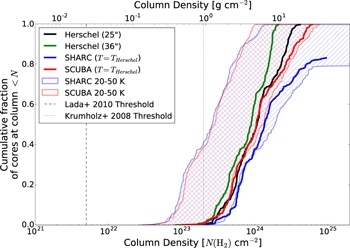
Figure 13. Cumulative distribution functions of the background column density associated with each identified 3 mm continuum source. The column densities are computed from a variety of maps with different resolution and assumed temperature. The Herschel maps use SED-fitted temperatures (C. Battersby et al. 2018, in preparation) at 25″ resolution (excluding the 500  data point) and 36″ resolution. The SHARC 350
  and SCUBA 450
  maps both have higher resolution (
 ) but no temperature information; we used an assumed
  K and
K and  K to illustrate the range of possible background column densities (hatched red and blue, respectively). The thick solid red and blue lines show the SHARC and SCUBA column density images using Herschel temperatures interpolated onto their grids: these curves are closer to the 20 K than the 50 K curve and serve as the best-estimate column density maps. The SHARC data fail to go to a cumulative fraction of 1 because the central pixels around Sgr B2 M and N are saturated (the lower-temperature assumptions result in optical depths
  , which cannot be converted to column densities using the optically thin assumption). The vertical dashed line shows the
  column density threshold from LLA10, and the vertical dotted line shows the the
  Krumholz & McKee (2008) threshold for high-mass star formation.
Download figure:
Standard image High-resolution image
LLA10 suggested that their observed column density threshold corresponds to a density n ≈ 104  . If we assume that the dense part of the Sgr B2 cloud is approximately a
  box (i.e., we assume that the depth is equal to the shortest observed dimension on the sky), the typical column density
  requires a mean density
  (which is a lower limit; most of the mass is at higher column densities). Again, effectively all of the gas associated with ongoing star formation is above the locally determined threshold.
To compare Sgr B2 to the LLA10 sample on a full-cloud scale, we can use the total cloud mass and total YSO mass. LLA10 used a YSO count, NYSO, while we infer a total YSO mass; we use their assumed median mass 
 to convert our observed MYSO to NYSO. Using their fitted relation for local clouds,36
 , we predict that for
  (where we use the whole cloud mass because all of the cloud is at
  ),
),  . As seen in Table 2, the observed
  , a factor of three to six below the extrapolated LLA10 relation. If we invert the equation to obtain a cloud mass from our observed
  , we would predict
  , which is equivalent to the mass in Sgr B2 above a column density threshold
  (Figure 14).
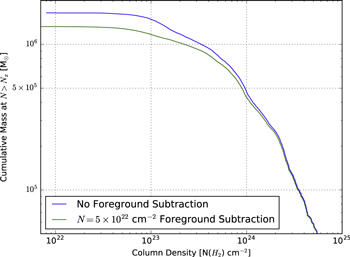
Figure 14. Cumulative mass above a threshold column density in the observed region. The two curves show the mass inferred with and without a foreground of  , the highest plausible foreground column density, subtracted.
Download figure:
Standard image High-resolution imageAny way we examine our data, it appears that a higher column density threshold for star formation is required in Sgr B2 than in local clouds. The one remaining caveat is that the LLA10 study used Spitzer observations of nearby clouds that were nearly complete to stars at least as small as 0.5  . By contrast, as discussed in Section 3.3.5, our survey is sensitive only to stars with
  . It is therefore possible that we have instead observed a higher threshold for high-mass star formation than for low-mass star formation (e.g., as suggested by Krumholz & McKee 2008).
4.3.2. Other Thresholds
A theoretical threshold for high-mass star formation,  (
( ), was developed by Krumholz & McKee (2008). Nearly all of the sources we have detected reside above this threshold (independent of the assumed foreground contamination), and we determined that our sources are all likely to be massive YSOs in Section 3.3.5. However, not all pixels with
  are forming high-mass stars (Figure 15). It appears that there is a threshold, but it is a necessary, not a sufficient, criterion for high-mass star formation.
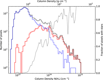
Figure 15. Histograms of the column density measured with the combined SCUBA and Herschel data using the interpolated Herschel temperatures covering only the region observed with ALMA. The black histogram (left axis) shows the whole observed region, the blue solid line shows the SCUBA pixels that do not contain an ALMA source, and the red thick line shows those pixels that are within one beam FWHM of an ALMA source. The thin black line (right axis) shows the ratio of the red histogram to the black histogram, i.e., it shows the fraction of pixels with associated YSOs. While the ALMA sources (high-mass YSOs) clearly reside in high column density gas, there is abundant high column density material that shows no signs of ongoing star formation.
Download figure:
Standard image High-resolution imageHowever, there is another threshold in our data,  , above which the majority of the gas is associated with ongoing high-mass star formation (Figure 15). This threshold suggests that any gas reaching a column density
  over a ≈0.5 pc size scale (the resolution of our column density maps) has more likely begun to form high-mass stars. This column density corresponds to a volume density
  assuming spherical symmetry.
4.3.3. Comparison to G0.253+0.016
In G0.253+0.016 (The Brick, G0.253), very little star formation has been observed (Longmore et al. 2013b; Johnston et al. 2014; Rathborne et al. 2014, 2015) despite most of the cloud existing above the locally measured LLA10 column density threshold. The column density distribution for G0.253 is shown in Figure 16.
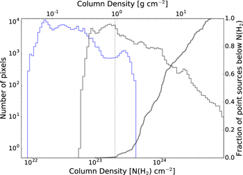
Figure 16. Histograms of the column density of G0.253+0.016 (blue) and Sgr B2 (gray) using the combined SCUBA 450  and Herschel 500
  intensity with the interpolated Herschel dust temperatures. The cumulative distribution of core “background” column densities in Sgr B2 is shown as a thick gray line, showing that the densities at which stars are forming in Sgr B2 are barely reached in G0.253. The vertical dotted line is the Krumholz & McKee (2008) threshold for high-mass star formation at
  , while the Lada et al. (2010) threshold is below the minimum value plotted here (see Section 4.3).
Download figure:
Standard image High-resolution imageThe Rathborne et al. (2014, 2015) ALMA 3 mm data are the deepest observations of G0.253 in the millimeter regime to date, with a sensitivity about  better than ours, but with a beam of 1
7 (similar to that shown in Figure 1; compare to Figure 2 in both Rathborne et al. papers). Despite the higher sensitivity of their data, they detected only three compact continuum sources. Similarly, Kauffmann et al. (2013) detected only one compact continuum source in their (less sensitive) SMA data. By contrast, even in our coarse resolution data, which have a worse sensitivity (rms ≈ 0.25 mJy beam−1,
 worse than Rathborne et al.), dozens of compact sources are evident. Our better resolution was critical for identifying the hundreds of sources we have identified, but it is nonetheless clear that the star formation activity is much higher in Sgr B2 than G0.253.
Comparing Sgr B2 to G0.253, the majority of the Sgr B2 cloud is at higher column than G0.253. Star formation in Sgr B2 nearly all occurs at a higher column than exists within G0.253 (Figure 16). The dearth of observed cores in G0.253 is therefore easily explained if there is a density threshold for star formation that is not reached in G0.253. Given that the G0.253 observations were deeper than our own, yet still identified almost no forming stars, it appears more likely that there is a lack of star formation rather than simply a lack of high-mass star formation. Nonetheless, robust verification of this hypothesis will require much deeper observations sensitive to low-mass stars in both regions.
4.4. Surface Density Relations: Comparison to Gutermuth et al. 2011
Unlike Lada et al. (2010), who invoke a threshold followed by a linear star formation law relating the gas to the stellar surface density, Gutermuth et al. (2011) concluded that star formation was best represented as power-law relations between the stellar and gas mass surface densities.
In this section, we measure the stellar surface density (Section 4.4.1) and compare the star–gas surface density relation to the local clouds observed by Gutermuth et al. (2011, Section 4.4.2), finding that the local clouds and Sgr B2 do not fit on a common relation. We examine the possible reasons for the disagreement (Section 4.4.3), concluding that a varying volume density threshold for star formation is the most likely explanation.
4.4.1. Methodological Comparison to Gutermuth et al.
We adopt the same approach used in Gutermuth et al. (2009, 2011) to compare gas and stellar mass surface densities. We computed both the star-centric mass surface density using the 11th-nearest-neighbor density and a gridded surface density. We assume a mean mass per source  and that each such star represents 23% of the total stellar mass (see Section 4.1), i.e., each 3 mm source is treated as a “cluster” containing 95
  of stellar mass.37
The correlation is similar whether we use the Herschel column density directly or the SCUBA- or SHARC-based column density maps (see Section 2.2).
of stellar mass.37
The correlation is similar whether we use the Herschel column density directly or the SCUBA- or SHARC-based column density maps (see Section 2.2).
There are a few key differences between our data and those of Gutermuth et al. (2011). First, our minimum detected column density is  , while in their sample, the maximum observed was AV = 38, or
  . Even if we subtract our upper-limit foreground estimate
  from the entire Sgr B2 map, nearly all of the detected sources reside in regions with column densities well above the maximum reached in the local cloud sample. Second, our 3 mm source sample is sensitive to only the youngest sources, either the high-mass equivalent of Class 0/I sources (“hot cores” or high-mass YSOs) or deeply embedded hypercompact H ii regions. The Spitzer sample included both Class I sources, with estimated ages
  , and Class II sources, with ages
  . Our sample is therefore biased young compared to theirs. If the age estimate for Sgr B2 from the dynamical models (Kruijssen et al. 2015) is accurate, there should be about as many Class II sources as Class I, given the standard ages, meaning that our total stellar mass estimate may be as much as a factor of 2 underestimated. Third, as noted above, we are sensitive to only high-mass sources, so we infer a significant population that is not directly observed.
We computed star formation relations following Gutermuth et al. (2011), Section 4.1. We use their Equation (7):
where  is the time-dependent stellar surface density, c is a scaling constant (assumed to be the star formation efficiency of a core and to have the value 0.3),
  is the initial gas surface density, t0 is the timescale for the gas to be depleted by
  ,
,  , and α is the exponent in the star formation relation (
 ). The depletion timescale t0 is defined by their Equation (5):

where k is the SFR coefficient. The constant k has different units depending on which value of α is adopted; for  , k has units of pc2
  −1 Myr−1.
If  , i.e., the SFR is proportional to the initial gas surface density, the surface density relation is instead
 ![${{\rm{\Sigma }}}_{* }(t)=c{{\rm{\Sigma }}}_{\mathrm{gas},0}[1-{e}^{-{kt}}]$](https://content.cld.iop.org/journals/0004-637X/853/2/171/revision1/apjaaa6d4ieqn314.gif) and the 50% depletion timescale is
and the 50% depletion timescale is  . The constant k is then the inverse star formation timescale with units of Myr−1.
4.4.2. Results of the Comparison to Gutermuth et al.
Figure 17 shows the stellar mass surface density  plotted against the gas mass surface density
  . Our data show a large scatter and are plausibly compatible with a power-law index in the range 1–2, and therefore they may be consistent with the steep slopes (
 ) Gutermuth et al. (2011) derived. Lada et al. (2017) and Lombardi et al. (2014) derived similarly steep slopes (
 for Orion,
  for the California cloud; see Appendix F).
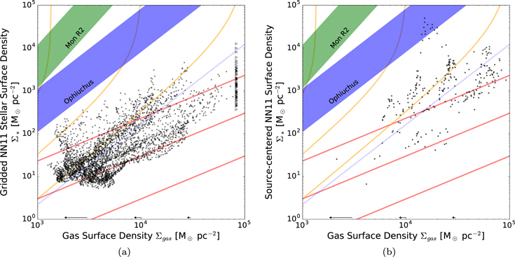
Figure 17. Plots of the protostellar mass surface density vs. the gas mass surface density as derived from Herschel SED fitting (Section 2.2). The stellar mass surface densities are computed using the 11th-nearest-neighbor distance assuming that each star represents a mass of 95  , extrapolated assuming a uniform IMF. Panel (a) shows the densities computed on a 0.25 pc grid, with column density lower limits indicated where the Herschel data are saturated, while panel (b) shows the protostar-centric surface densities; no lower limits are included in this figure because interpolated mass surface densities are used instead. The shaded regions show the extrapolations of the relations derived by Gutermuth et al. (2011) for Ophiuchus (blue) and Mon R2 (green); their data cut off below a mass surface density
 pc−2. The blue dotted line shows the Ophiuchus relation scaled down by
  to overlap with our data. The thick orange lines show realizations of the Gutermuth et al. (2011)
  star formation relation at times 0.01, 0.1, and 0.74 Myr, from bottom to top. Similarly, the thick red lines show realizations of the
  star formation relation at the same ages. The arrows along the bottom show the effect of subtracting a uniform foreground column density of
  (1100
(1100  pc−2).
Download figure:
Standard image High-resolution imageFigure 17 shows in orange three curves from the Gutermuth et al. (2011)  star formation relation, their Equation (7) (our Equation (3)), with
  pc2
pc2  −1 Myr−1 and
  , at times t = 0.01, 0.1, and 0.74 Myr. Only the youngest curve, with age 0.01 Myr, overlaps with our data. The three red curves, which are essentially lines in this figure, show the
  relation with k = 0.1 Myr−1 at the same three ages, and they achieve reasonable agreement with our data for the t = 0.74 Myr line (k = 0.1
  implies the 50% depletion time
  Myr). The
  star formation relation is only consistent with our data for times earlier than
  . This inconsistency is due to the very fast depletion time for this form of star formation relation, which decreases with gas surface density. Indeed, the
  star formation relation used by Gutermuth et al. (2011) is completely implausible for the gas surface density regime we observe, as it implies that gas with an initial surface density of
  would achieve a star formation efficiency
  in
in  . While our data are clearly incompatible with the
  relation, they are reasonably compatible with a linear
  relation with the same normalization used by Gutermuth et al. (2011), i.e., k = 0.1 Myr−1.
Figure 17 also shows that the extrapolated relation from the low-mass clouds exceeds our observations by at least  (Ophiuchus) or closer to
  (Mon R2). The discrepancy between our observations and theirs indicates either that there is a systematic tendency to overestimate
  at high
  in the Spitzer observations, which seems unlikely, or that there is a different star formation–gas surface density relation in Sgr B2 and in local clouds.
4.4.3. A Critical Evaluation of the Discrepancies with Gutermuth et al.
While a linear relation  can approximately account for both local clouds and Sgr B2 as a whole, we have not yet explained why the extrapolation of the observed
  relation from local clouds does not match Sgr B2. We evaluate several possibilities here:
- 1.Could we be missing an older generation? Gutermuth et al. (2011) were sensitive to, and included in their sample, an older generation of Class II sources, which we cannot detect. However, they typically found a Class II/Class I ratio of only (Gutermuth et al. 2009) (and they found that this ratio decreased at higher gas surface densities), so the discrepancy cannot be exclusively due to our insensitivity to older YSOs unless the SFR within Sgr B2 was an order of magnitude higher 1–5 Myr ago. Such an enhanced SFR is implausible since such a large population of massive stars would still be alive and very easily detectable in our survey and previous VLA surveys.
- 2.Could we be overestimating the gas mass? The surface densities we measure cannot be substantially incorrect. Even if we assume the maximum plausible foreground cloud surface density of, the measured gas surface densities only shift by a small fraction (at most 50%, but typically for the star-centered measurements; see the arrows in Figure 17). If the dust opacity or dust-to-gas ratio were substantially wrong, e.g., if the dust-to-gas ratio is 10 instead of 100, some of our data would begin to overlap with the local cloud data. If we had overestimated the gas mass by the required amount to bring our data into agreement with the local clouds, the star formation efficiency would be close to 50% (i.e., ), which is unlikely given the many signs of youth observed.
- 3.Could there be high multiplicity in our sample? A possible explanation is that each of the detected sources in our sample is a high-number multiple system, such that each 3 mm source represents ≈5000 instead of ≈100 . The multiplicity of the Orion Source I system suggests that this interpretation is qualitatively plausible, but the factor of 50 required to match the extrapolation of the Gutermuth et al. (2011) data strains credibility. Additionally, the luminosity constraints from our observed data rule this possibility out unless the stellar IMF is bottom-heavy (see below for more IMF discussion).
- 4.Could the sources be much more massive than we have inferred? Another possibility is that each source we detect has a higher minimum mass than we have assumed,, but again the required threshold is absurd, requiring each star to be to match the local cloud extrapolation. Such massive stars are incompatible with the observed 3 mm luminosities for any plausible dust envelope or H ii region model (see Section 3.3).
- 5.Could our sample be incomplete? If our sample were incomplete by a factor of 100–1000, our results would match those extrapolated from Gutermuth et al. While Section 3.1 concedes that the catalog may be incomplete, it is unlikely that we are complete, and the catalog is almost certainly complete to for very massive and luminous sources (; see Section 3.3.5). Additionally, if we were to include a factor of 100–1000 more stellar mass, the implied total stellar mass would be absurd, reaching , exceeding the cloud mass.
- 6.Could Sgr B2 consist of several Mon R2-like clouds stacked along the line of sight? If there were ∼50–100 clouds of the same physical scale and surface density stacked along the line of sight, the data in Figure 17 would shift left, providing a possible explanation of the difference. However, besides the extreme unlikeliness of having so many clouds along the line of sight, this explanation would require that the majority are non-star-forming, i.e., they would have to be extremely young. Also, the observations do not favor this scenario, as most of the star formation appears associated with a single velocity component in the data (e.g., Figure 8, Appendix D). Finally, the elongation of the cloud on the sky hints that it is not multiple clouds, since they would have to all have similar elongations.
- 7.Is the stellar IMF spatially nonuniform? Our stellar mass surface density measurements are predicated on the assumption that each high-mass YSO represents a fully sampled IMF at the same location. If there is any spatial nonuniformity in the IMF, e.g., if massive stars preferentially form at the bottoms of large potential wells (“primordial mass segregation”), the massive stars will have a different spatial distribution than the low-mass stars. This effect would result in a higher measured stellar surface density at the highest gas surface densities and a lower measured stellar surface density at the lowest gas surface densities, i.e., it would result in a steeper slope in Figure 17. Therefore, unless there is inverse mass segregation, a spatially nonuniform IMF cannot explain our observations.
- 8.Is the stellar IMF temporally nonuniform? If high-mass stars form first, we would overestimate the stellar mass surface density. However, if low-mass stars form first, we could underestimate the stellar mass surface density. Given our survey’s insensitivity to low-mass YSOs, the stellar mass surface density could be over an order of magnitude higher if it consists only of low-mass YSOs. Such a dramatic time-sequencing effect in star formation would have profound implications for star formation studies, implying that any or all clouds currently forming low-mass stars may eventually form higher-mass stars, so testing this possibility with high-sensitivity observations should be a priority.
- 9.Is the local star formation efficiency lower at a fixed surface density in the Galactic center? The overall SFR in the Galactic center is lower than expected given predictions from local clouds. Changing the normalization of the star formation relation, i.e., reducing the prefactor c = 0.3 to c = 0.01, where c is the fraction of gas in a core that makes it onto a star (the local efficiency), would allow our results to be consistent. However, there is no evidence for any difference in the star formation process in the Galactic center once a core has formed; most evidence currently points to inefficient core formation in the CMZ.
- 10.Could the high star formation threshold in the CMZ explain the difference? As noted in Sections 4.3.1 and 4.3.2 above, forming stars only begin to appear above a threshold significantly higher than in local neighborhood clouds. A simplistic model in which star formation simply does not occur below a fixed column threshold does not explain the difference between our data and Gutermuth’s, however, because the disagreement occurs at the high column densities in which we do observe star formation. On the other hand, a higher volume density threshold is plausible. Such a threshold would imply a lower stellar density at a given surface density and would permit variations in the stellar surface density depending on how much dense gas is present.


Of the items above, only the final one, which suggests that a surface-density-based star formation law is inviable, satisfactorily explains the discrepancy between our data and the extrapolation from Gutermuth et al. (2011).
4.5. Interpretation of a Varying Threshold for Star Formation
In Sections 4.3 and 4.4, we concluded that a varying star formation density threshold is likely to exist in the CMZ. Other authors have come to the same conclusion based on observations of G0.253+0.016 (Kruijssen et al. 2014; Rathborne et al. 2014). Here, we briefly discuss what may drive such a varying threshold.
Federrath & Klessen (2012) summarized and reformulated a variety of turbulence-based star formation theories. These theories assume that the gas density in a molecular cloud is approximately lognormally distributed, with the distribution’s shape parameters governed by turbulent parameters, the most important being the mean Mach number of the cloud. In the models, gas above some threshold density ncrit becomes gravitationally unstable and collapses to form stars. The three models (Krumholz et al. 2005; Hennebelle & Chabrier 2011; Padoan & Nordlund 2011b) have different threshold criteria. Most importantly, the Krumholz et al. (2005) and Padoan & Nordlund (2011b) threshold densities rise with increasing Mach number ( ), while the Hennebelle & Chabrier (2011) threshold decreases with Mach number (
 ). Since our observations imply the need for a higher threshold density, and Galactic center clouds are more turbulent (higher Mach number) than local clouds (e.g., Federrath et al. 2016), the Hennebelle & Chabrier (2011) model is qualitatively inconsistent with our observations.
5. Conclusions
We have reported the detection of 271 3 mm point sources in the extended Sgr B2 cloud and determined that the majority are high-mass protostellar cores. This survey represents the first large population of YSOs detected in the Galactic center and the largest sample yet reported of high-mass YSOs.
The large population of high-mass protostellar cores indicates that an extended region spanning the entire Sgr B2 cloud, not just the well-known clusters N, M, and S, is undergoing a burst of star formation. More than half of the currently forming generation of stars is not associated with any of the clusters but is instead part of the extended burst.
Using Herschel, SCUBA, and SHARC data, we have observed a threshold for high-mass star formation analogous to that inferred in local clouds by Lada et al. (2010). We find that there are no high-mass YSOs in gas below  at a resolution of
  (0.4 pc), and half of the detected sources are found above
  . However, there is abundant material above
  that has no associated YSOs, indicating that this threshold is a necessary but not sufficient criterion for high-mass star formation. These measurements imply either the existence of a higher threshold for high-mass star formation than for low-mass star formation, as predicted by several theories (e.g., Krumholz & McKee 2008), or a higher threshold for star formation in the Galactic center as compared to local clouds (e.g., as proposed by Kruijssen et al. 2014; Rathborne et al. 2014). Deeper observations recovering the low-mass sources are required to distinguish these possibilities.
Comparing the protostellar mass surface density to the gas mass surface density revealed a correlation compatible with the slopes observed by Gutermuth et al. (2011), but with an amplitude significantly inconsistent with theirs. A star formation relation of the form  with
with  favored by Gutermuth et al. (2011) cannot explain our observations, though an
  (linear) relation is consistent with our data, and the
  relation implies an age
  that is consistent with the Kruijssen et al. (2015) dynamical model age for the Sgr B2 cloud
  .
.
The extrapolation of the surface density relations from local clouds in Gutermuth et al. (2011) does not agree with our data. We explored a wide variety of possible explanations for the difference and concluded that the most likely is that a surface density relation is incapable of explaining both local and CMZ clouds. Instead, a volume-density-based model, in which the volume density threshold is higher in the CMZ, may be viable.
The large detected population of high-mass YSOs implies a much larger population of as-yet-undetectable lower-mass YSOs. Future ALMA and JWST programs to probe this population would provide the data needed to directly compare star formation thresholds in the most intensely star-forming cloud in our Galaxy with those in nearby clouds.
We thank the anonymous referee for a very constructive and helpful report. The National Radio Astronomy Observatory is a facility of the National Science Foundation operated under cooperative agreement by Associated Universities, Inc. This paper makes use of the following ALMA data: ADS/JAO.ALMA#2013.1.00269.S. ALMA is a partnership of ESO (representing its member states), NSF (USA), and NINS (Japan), together with NRC (Canada), NSC and ASIAA (Taiwan), and KASI (Republic of Korea), in cooperation with the Republic of Chile. The Joint ALMA Observatory is operated by ESO, AUI/NRAO, and NAOJ. This work is partly supported by a grant from the National Science Foundation (AST-1615311, De Pree). J.M.D.K. gratefully acknowledges funding from the German Research Foundation (DFG) in the form of an Emmy Noether Research Group (grant no. KR4801/1-1), from the European Research Council (ERC) under the European Union’s Horizon 2020 research and innovation program via the ERC Starting Grant MUSTANG (grant agreement no. 714907), and from Sonderforschungsbereich SFB 881 “The Milky Way System” (subproject P1) of the DFG. R.G.-M. acknowledges support from UNAM-PAPIIT program IA102817. J.C. acknowledges support for this work provided by the NSF through the Grote Reber Fellowship Program administered by Associated Universities, Inc./National Radio Astronomy Observatory. A.S.-M., P.S., and F.M. are partially supported by Deutsche Forschungsgemeinschaft through grant SFB956 (subproject A6). J.E.P. acknowledges the financial support of the European Research Council (ERC; project PALs 320620).
Software: The software used to make this version of the paper is available from github at https://github.com/keflavich/SgrB2_ALMA_3mm_Mosaic/ with hash e26ce0f(2017-12-28). The tools used include spectral-cube, radio-beam, and uvcombine from the radio-astro-tools package (https://github.com/radio-astro-tools/spectral-cube, (https://github.com/radio-astro-tools/radio-beam, (https://github.com/radio-astro-tools/uvcombine, and radio-astro-tools.github.io), astropy (Astropy Collaboration et al. 2013), astroquery (astroquery.readthedocs.io), and CASA (McMullin et al. 2007).
Appendix A: Single-dish Combination
To measure the column density at a resolution similar to that of Lada et al. (2010), we needed to use ground-based single-dish data with resolution  . We combined these images with Herschel data, which recover all angular scales, to fill in the missing “short spacings” from the ground-based data.
Specifically, we combine the SHARC 350  (Dowell et al. 1999) and SCUBA 450
  (Pierce-Price et al. 2000; Di Francesco et al. 2008) with Herschel 350 and 500
  data (Molinari et al. 2016), respectively.
Combining single-dish with “interferometer” data, or data that are otherwise insensitive to large angular scales, is not a trivial process. The standard approach advocated by the ALMA project is to use the “feather” process, in which two images are Fourier-transformed, multiplied by a weighting function, added together, and Fourier-transformed back to image space (see equations in Section 5.2 of Stanimirovic 2002). This process is subject to substantial uncertainties, particularly in the choice of the weighting function.
Two factors need to be specified for linear combination: the beam size of the “single-dish,” or total power, image, and the largest angular scale of the “interferometer” or filtered image. While the beam size is sometimes well known, for single dishes operating at the top of their usable frequency range (e.g., the CSO at 350  or GBT at 3 mm), there are uncertainties in the beam shape and area and there are often substantial sidelobes. In interferometric data, the largest angular scale is well defined in the originally sampled UV data but is less well defined in the final image because different weighting factors change the recovered largest angular scale. For ground-based filtered data, the largest recoverable angular scale is difficult to determine (e.g., Chapin et al. 2013; Ginsburg et al. 2013).
To assess the uncertainties in image combination, particularly on the brightness distribution (e.g., Ossenkopf-Okada et al. 2016), we have performed a series of experiments combining the Herschel with the SCUBA data using different weights applied to the SCUBA data. As discussed in Section 2, we empirically determined that the scale factor required for the best match between SCUBA and Herschel data was  , which is large but justifiable. In the experiment shown in Figure 18, we show the images and resulting histograms when we combine the Herschel data with the SCUBA data scaled by a range of factors from
  to
to  . The changes to the high end of the histogram are dramatic, but the middle region containing most of the pixels (and most relevant to the discussion of thresholds in the paper) is not substantially affected. Additionally, we show the cumulative distribution function of core background surface brightnesses (as in Figure 13), showing again that only the high end is affected.
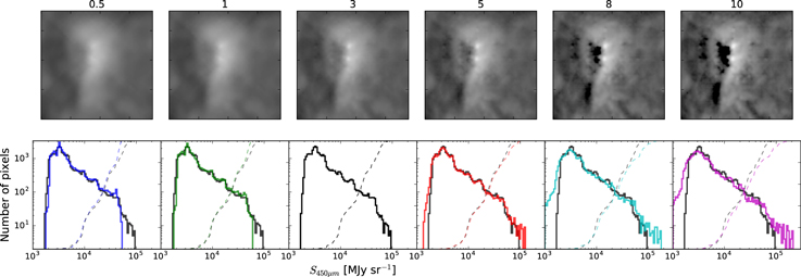
Figure 18. Demonstration of the effects of using different calibration factors when combining the SCUBA data with the Herschel data using the “feather” process. The numbers above each panel show the scale factor applied to the SCUBA data before Fourier-combining it with the Herschel data. The factor of 3 was used in this paper and shows the most reasonable balance between the high resolution of the SCUBA data and the all-positive Herschel data. In the lower panels, the fiducial scale factor of 3 is shown in black in all panels. The solid lines show histograms of the images displayed in the top panels. The dashed lines show the cumulative distribution of the background surface brightnesses of the point sources in this sample; they are similar to the distributions shown in Figure 13.
Download figure:
Standard image High-resolution imageAppendix B: Self-calibration
We demonstrate the impact of self-calibration in this section. The adopted approach used three iterations of phase-only self-calibration followed by two iterations of phase and amplitude self-calibration. Each iteration involved slightly different imaging parameters. The final, deepest clean used a threshold mask on the previous shallower clean. The script used to produce the final images is available at https://github.com/keflavich/SgrB2_ALMA_3mm_Mosaic/blob/e26ce0f/script_merge/selfcal_continuum_merge_7m.py. The effects are shown with a cutout centered on the most affected region around Sgr B2 M in Figure 19.
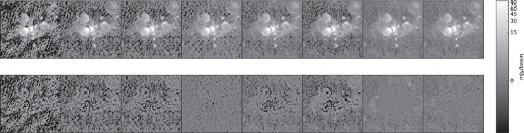
Figure 19. Progression of the self-calibration iterations. The images show, from left to right, the initial image; one, two, and three iterations of phase-only self-calibration; two iterations of phase and amplitude self-calibration; a reimaging of the fifth iteration with a deeper 0.1 mJy threshold using a mask at the 2.5 mJy level; and finally, a sixth iteration of phase and amplitude self-cal cleaned to 0.1 mJy over a region thresholded at 1.5 mJy. All imaging was done using two Taylor terms and multiscale clean. The second row shows the corresponding residual images.
Download figure:
Standard image High-resolution imageAppendix C: Photometric Catalog
We include the full catalog in digital form (https://github.com/keflavich/SgrB2_ALMA_3mm_Mosaic/blob/master/ta-bles/continuum_photometry_withSIMBAD_andclusters.ipac). Table 3 shows the brightest 35 sources; the rest are included in a digital-only catalog. Sources are labeled based on an arbitrary source number plus any preexisting catalog name. If a source is associated with a cluster, it has an entry corresponding to that cluster in the Cluster column; association is determined by checking whether a source is within a particular distance of the cluster center as defined by Schmiedeke et al. (2016). A source Classification column is included, which states whether the source is a strong or weak detection, whether it has an X-ray association, whether it has a maser association, and its SIMBAD classification if it has one. Measurements reported include the peak flux density  , the corresponding brightness temperature
  , the integrated flux density within a beam (0
5) radius, the background rms flux level
 as an estimate of the local noise, the spectral index α, and the error on that
  . Mass and column density estimates are given for an assumed temperature T = 40 K (M40 K and
  ). For sources with
  K, these estimates are unlikely to be useful since the assumed temperature is probably lower than the true temperature. For sources with
  K, it is not possible to measure a mass assuming T = 40 K, so those entries are left empty.
Appendix D: Additional Figures Showing

The  line was discussed at various points in the paper. Because the data are extremely rich and complex, we include some additional figures (Figures 20 and 21) showing the detailed structure of the lines here.
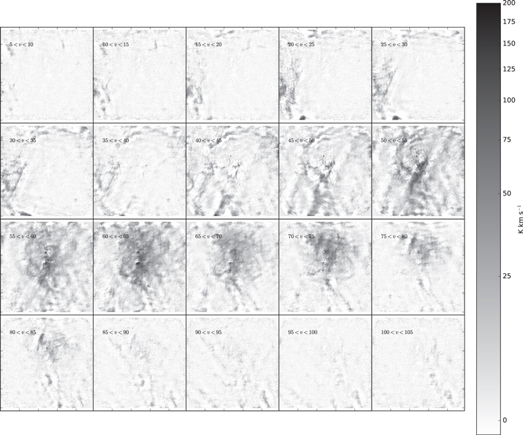
Figure 20. Channel maps of the  J = 10–9 line. Each panel shows the integrated intensity over a 5
  velocity range as indicated in the figures. The data shown here are 12 m+7 m images made excluding the long-baseline data sets to emphasize large angular scales combined with total power data by feathering the images. The “ridge” feature discussed in the text is most evident in the 50–55
  channel, and these images show that it is dominated by a single velocity component.
Download figure:
Standard image High-resolution image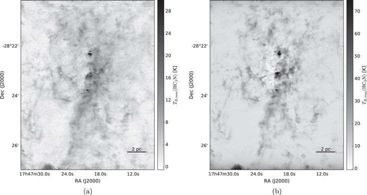
Figure 21. Peak-intensity maps of  J = 10–9. The left panel shows the 12 m short-baseline data combined with 7 m and total power data; by excluding the long-baseline data, the large angular scales are emphasized. The right panel shows the robust 0.5-weighted 12 m+7 m data combined with total power data; it reaches a substantially higher peak intensity in the compact regions, but the lower-intensity diffuse emission is relatively hidden. In the right panel, the negative bowls seen near Sgr B2 M and N in this peak-intensity image indicate that intermediate size scales were not well recovered. The bright feature on the lower left of both images may be an imaging artifact.
Download figure:
Standard image High-resolution imageAppendix E: Additional Figure Showing Sgr B2 M and N
We show the Sgr B2 M and N source identifications overlaid on VLA 1.3 cm continuum (De Pree et al. 2014) in Figure 22. This figure highlights the differences between the wavelengths and provides a visual verification that our classification of sources as H ii regions is reasonable.
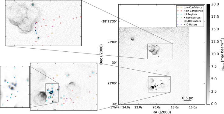
Figure 22. Close-up of Sgr B2 M and N, similar to Figure 3, but with VLA 1.3 cm continuum (De Pree et al. 2014) in the background instead of the ALMA 3 mm continuum. Many of the features that appear in the 3 mm image do not appear in the 1.3 cm image and are likely to be from dust emission, but the poorer sensitivity of the 1.3 cm data also suggests that some of these features are simply free–free emission undetected at 1.3 cm.
Download figure:
Standard image High-resolution imageAppendix F: Star–Gas Surface Density Figure with Lada et al. 2017 Relations
We show in Figure 23 a version of Figure 17 with the extrapolated relations from the Orion A, Orion B, and California molecular clouds overlaid. Similar to the comparison to Gutermuth et al. (2011) in Section 4.4.2, the Lada et al. local clouds extrapolate to significantly higher stellar mass surface densities than we observe in Sgr B2.
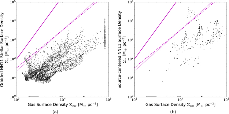
Figure 23. Same as Figure 17, but with the models and Gutermuth et al. clouds removed and extrapolations from the California (solid magenta), Orion A (dashed magenta), and Orion B (dotted magenta) clouds overlaid. As for the other local clouds, there is no overlap in the X-axis between our observations and theirs, so the plotted relations are pure extrapolation.
Download figure:
Standard image High-resolution imageFootnotes
- 23
Reid et al. (2014) also conclude that the distance to the Galactic center is 8.34 kpc, suggesting that the direct parallax measurement to Sgr B2 is underestimated.
- 24
Other lines targeted include CH3CN 5–4, HCN 1–0, HNC 1–0, HCO+ 1–0, H41α, and
. - 25
- 26
We assume a gas-to-dust ratio of 100 throughout this work.
- 27
We consider a source unresolved if its radius is smaller than the Gaussian width of our beam,
, rather than the FWHM of , since a source with the latter width would be measurably extended when convolved with the beam. - 28
We use the tabulations of OB star properties from Vacca et al. (1996) and Pecaut & Mamajek (2013), via their online table http://www.pas.rochester.edu/~emamajek/EEM_dwarf_UBVIJHK_colors_Teff.txt, to determine the relation between spectral type, luminosity, and mass.
- 29
Assuming that all 50 sources with
mJy are massive stars with , only 17 stars in the range 8–10 are expected assuming a Kroupa (2001) IMF. - 30
- 31
We err on the shallower side, implying that the extrapolated 3 mm fluxes are brighter than they should be, since this approach gives a more conservative view of the detectability of the Orion sources. In reality, such sources are likely even fainter than predicted here.
- 32
This source includes Source I, BN, and a few other objects at this resolution, and at 3 mm Source I and BN are comparably bright (Plambeck et al. 2013). This source is not part of the HOPS sample.
- 33
At the
level, up to 11 sources are consistent with , but this is primarily because of their high measurement error. - 34
We use the higher of the two masses out of
and for each row because, as discussed in Section 4.2, Sgr B2 M likely has an underestimated , either due to observational effects such as confusion or because it is older and the more moderate-mass sources represented by the cores have become unobservable. Similarly, the unassociated sources appear to be younger, and therefore the H ii-region-based mass appears to be an underestimate. - 35
Column density is commonly used as a proxy for volume density because of its observational convenience, but volume density is the more meaningful physical parameter for most relevant processes in star formation (e.g., gravity and pressure).
- 36
In the main body of their paper, Lada et al. included all YSOs in the clouds down to
for their total YSO counts. However, in the text they repeated their NYSO–Mcloud fit using only stars embedded in gas with . They obtained a linear relation about 0.6× lower than that shown in their paper (C. Lada 2018, private communication). The better agreement when including only embedded YSOs hints that the discrepancy noted in this section could disappear if a complete census of Class II sources were obtained in Sgr B2. - 37
In previous sections, we assigned different masses to different source classes, i.e., we assigned higher masses to H ii regions than non-H ii regions. For consistency with Gutermuth et al. (2011), we assume a constant mass per source here, which may result in a systematic underestimation of the stellar mass surface density at the highest densities (since the H ii regions are preferentially concentrated in clusters).


