Abstract
Anisotropic stochastic gravitational wave background (SGWB) serves as a potential probe of the large-scale structure (LSS) of the universe. In this work, we explore the anisotropic SGWB from local (z < ∼ 0.085) merging stellar mass compact binaries, specifically focusing on merging stellar binary black holes, merging neutron star–black hole binaries, and merging binary neutron stars. The analysis employs seven all-sky mock lightcone gravitational wave event catalogs, which are derived from the Millennium simulation combined with a semianalytic model of galaxy formation and a binary population synthesis model. We calculate the angular power spectra Cℓ at multipole moments ℓ, expressed as log10[ℓ(ℓ + 1)Cℓ/(2π)], based on the skymaps of the overdensity δGW in the anisotropic SGWB. The spectra for all three source types exhibit an approximately linear increase with log10ℓ at higher ℓ (e.g., ℓ > ∼ 30–300) in seven catalogs, with a characteristic slope of ∼2. The spectra of seven catalogs exhibit considerable variations, arising from fluctuations in spatial distribution, primarily in the radial distribution, of nearby sources (e.g., <50 Mpc h−1). After subtracting these nearby sources, the variations become much smaller and the spectra for the three source types become closely aligned (within discrepancies of a factor of ∼2 across ℓ = 1–1000 for all catalogs). We also find that including farther sources results in a rapid decrease in the anisotropy.
Original content from this work may be used under the terms of the Creative Commons Attribution 4.0 licence. Any further distribution of this work must maintain attribution to the author(s) and the title of the work, journal citation and DOI.
1. Introduction
Various gravitational wave (GW) sources, such as merging supermassive (M > 107M⊙) binary black holes (SMBBHs), merging stellar binary black holes (BBHs), merging neutron star–black hole binaries (NSBHs), merging binary neutron stars (BNSs), contribute to the total stochastic gravitational wave background (SGWB). For a summary of the sources, see recent reviews, e.g., N. Christensen (2019) and A. I. Renzini et al. (2022). Recently, pulsar timing array collaborations, including the European Pulsar Timing Array (J. Antoniadis et al. 2023), NANOGrav (G. Agazie et al. 2023a), Parkes Pulsar Timing Array (D. J. Reardon et al. 2023), and Chinese Pulsar Timing Array (H. Xu et al. 2023), have provided strong evidence for the existence of the SGWB. Furthermore, direct detections of merging BBHs, merging BNSs, and merging NSBHs (e.g., R. Abbott et al. 2023a) also suggest the presence of a potentially vast number of compact binary coalescences (CBCs) contributing to the SGWB. The anticipated detection of the SGWB by both ground-based detectors, such as the advanced Laser Interferometer Gravitational-Wave Observatory (G. M. Harry & LIGO Scientific Collaboration 2010) and the Einstein Telescope (ET; M. Punturo et al. 2010), and space-based detectors, such as the Laser Interferometer Space Antenna (P. Amaro-Seoane et al. 2017), is forthcoming, promising significant advancements in our understanding of the universe.
The SGWB can be divided into isotropic and anisotropic parts. Beyond the extensively studied isotropic part (e.g., R. Abbott et al. 2021; S. S. Bavera et al. 2022; G. Agazie et al. 2023b), the anisotropic part provides additional insights, particularly concerning the spatial distribution of GW sources. Several studies have explored the anisotropic SGWB; for example, the anisotropy from merging SMBBHs (C. M. F. Mingarelli et al. 2017; B. Bécsy et al. 2022; G. Agazie et al. 2023c; E. C. Gardiner et al. 2024; Q. Yang et al. 2024) and the anisotropy from merging BBHs, NSBHs, BNSs (G. Cusin et al. 2018; A. C. Jenkins et al. 2018, 2019a; G. Capurri et al. 2021). A. C. Jenkins et al. (2018) and A. C. Jenkins et al. (2019a) first use the mock lightcone GW event catalog to investigate the anisotropy of merging stellar-mass compact binaries. Specifically, they employ a postprocessing analytical approach to compute the GW events within the galaxies contained in the all-sky mock lightcone galaxy catalog sourced from J. Blaizot et al. (2005) and G. De Lucia & J. Blaizot (2007). However, their results suggest a significantly higher anisotropy level compared to the prediction of G. Cusin et al. (2018), particularly at very small scales. The discrepancies among these studies remain under discussion.
The GW event catalogs could be obtained from a semianalytic model of galaxy formation, Galaxy Assembly with Binary Evolution (GABE; Z. Jiang et al. 2019), combined with a rapid binary population synthesis model COSMIC v3.3.0 (K. Breivik et al. 2020a, 2020b). Using the binary population data generated by COSMIC, merging BNSs, NSBHs, and BBHs can be explored within the cosmological framework provided by GABE. For example, Z. Li et al. (2024) calculates the total SGWB from these sources using this GABE–COSMIC methodology. However, the original event catalog lacks information on the source positions within the celestial sphere. In this work, we use the original event catalog to construct seven all-sky mock lightcone GW event catalogs, which incorporate source position information across the celestial sphere, to investigate the anisotropic SGWB from the local (z < ∼ 0.085) merging BBHs, NSBHs, and BNSs.
The structure of this paper is as follows. In Section 2, we present the fundamental equations used to calculate the anisotropic SGWB and the angular power spectrum. Section 3 briefly outlines the GABE–COSMIC methodology to produce the GW event catalogs and details the methodology employed for generating mock lightcone GW event catalogs. The results, including the anisotropic SGWB and angular power spectra, are discussed in Section 4. Finally, the primary conclusions of the study are summarized in Section 5.
2. Formalism
2.1. Anisotropic SGWB from Ground-based Detector Compact Binaries
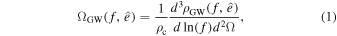
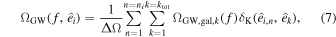
The SGWB from the observed direction  is defined by the dimensionless energy density (G. Cusin et al. 2017; A. C. Jenkins et al. 2018):
where  is the critical energy density and d3ρGW is the present-day energy density of GWs from the observed frequency interval {f, f + df} and the solid angle element d2Ω centered on
  . The ΩGW could be calculated using the Phinney formula (E. S. Phinney 2001) in the homogeneous and isotropic universe:
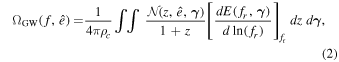
where  are intrinsic parameters of GW sources, such as the primary star mass m1 and the secondary star mass m2 of CBCs in this work;
  is the number of GW sources per comoving volume per redshift per intrinsic parameter range at observed direction
  ; and
; and 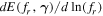 is the energy spectrum of a single GW source in logarithmic interval, f is the observed frequency, and fr = (1 + z)f is the frequency in the cosmic rest frame of the GW source. In this work, we adopt the same energy spectrum as used in X.-J. Zhu et al. (2011) and P. Ajith et al. (2008), assuming that this spectrum remains applicable for merging BNSs and NSBHs. By dividing the full-direction comoving element presented in E. S. Phinney (2001) by 4π, we can derive the comoving volume element at the observed direction
  as follows:
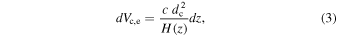
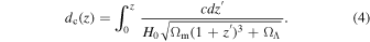
where ![$H(z)={H}_{0}{[{{\rm{\Omega }}}_{{\rm{m}}}{\left(1+z\right)}^{3}+{{\rm{\Omega }}}_{{\rm{\Lambda }}}]}^{0.5}$](https://content.cld.iop.org/journals/0004-637X/985/2/208/revision1/apjadca36ieqn9.gif) and dc is the comoving distance:
and dc is the comoving distance:
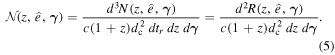
Using dz/dtr = (1 + z)H(z),  could be calculated using the merger rate of GW sources, defined by the number of mergers per source-frame time tr, in the comoving volume element in the intrinsic parameter element,
  , at observed direction
  :
:
We now extend the applicability of the above formulas to an inhomogeneous and anisotropic universe, assuming that all GW events occur within galaxies. Consequently,  and
and  might vary across different directions in accordance with the distribution of galaxies. By substituting Equation (5) into Equation (2), we compute the direction-dependent SGWB by summing the contributions from all galaxies within the galaxy catalog (similar to A. C. Jenkins et al. 2018):
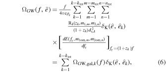
where m and n are the bin indices of the primary star mass m1 and the secondary star mass m2 of CBCs; m1cen and m2cen are the central values of m1 and m2 in each bin; and mtot and ntot are the total bin numbers of m1 and m2, respectively, which are determined by the division of the m1 × m2 space; k is the index of the galaxies; ktot is the total number of the galaxies in the catalog; Rk is the merger rate of merging stellar compact binaries in the galaxy k at zk in the primary mass-secondary mass bin Δm1, m2; δK is the Kronecker delta function;  is the direction of the galaxy k, and see Section 3.2 for details on the positions of our galaxies; and ΩGW,gal,k is the contribution of the galaxy k to the SGWB. In this work, the Rk is approximated as the mean merger rate in the galaxy k, denoted
  . Details regarding the calculation of
  can be found in Section 3. This study focuses exclusively on the anisotropy arising from the spatial distribution of GW sources. For a more comprehensive formalism that incorporates additional effects such as Doppler, Kaiser, and gravitational potential influences, see G. Cusin et al. (2017) and D. Bertacca et al. (2020). Note that some of these effects have a negligible impact on anisotropy. For example, the kinematic dipole resulting from the observer’s peculiar motion has been reported as minor (A. C. Jenkins et al. 2018; A. C. Jenkins 2022).
In this work, the skymaps are constructed as HEALPix6
maps (K. M. Górski et al. 2005) composed of Npix equal area pixels, where  is the number of pixels of the HEALPix skymap, with Nside denoting the parameter utilized in the HEALPix framework. A pixel may correspond to a range of directions, specifically
  ,
,  , ...,
  . In practice,
  is computed as follows:
where i denotes the index of the pixel corresponding to the observed direction  (
( associated with the ith pixel), ni is the total number of the directions within the pixel, and ΔΩ is the pixel area.
The overdensity δGW in the anisotropic SGWB from ground-based detector compact binaries is defined as follows (A. C. Jenkins et al. 2019a):
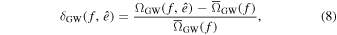
where 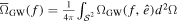 is the mean SGWB over the sky and
  is the surface of the celestial sphere.
2.2. Angular Power Spectrum
To quantify the anisotropy of the SGWB at various scales, the angular power spectrum Cℓ is adopted in this work. The angular power spectrum Cℓ quantifies the amplitude of statistical fluctuations in the angular power of the SGWB at scales θ ∼ 180∘/ℓ, where ℓ denotes the multipole moment. The Cℓ is calculated using the healpy package (K. M. Górski et al. 2005; A. Zonca et al. 2019). Below are its formulas (K. M. Górski et al. 2024). The overdensity δGW at each frequency on the celestial sphere can be expanded as:

where Ylm are spherical harmonics and:
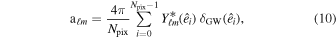
where i denotes the index of the pixel, and the superscript star is complex conjugation. Consequently, the angular power spectrum can be expressed as:

We calculate Cℓ up to  7
To maintain consistency with the previous literature, we multiply Cℓ by ℓ(ℓ + 1)/(2π). Note that using the angular power spectrum alone to describe the anisotropy implicitly assumes a stationary Gaussian random field for the SGWB. However, when considering the SGWB at a single frequency, along with the effective temporal observation window for ground-based GW detectors, additional non-Gaussianity might arise (A. C. Jenkins & M. Sakellariadou 2018; A. C. Jenkins et al. 2018). In future work, bispectrum and trispectrum analyses might be required to capture these complexities in greater detail.
7
To maintain consistency with the previous literature, we multiply Cℓ by ℓ(ℓ + 1)/(2π). Note that using the angular power spectrum alone to describe the anisotropy implicitly assumes a stationary Gaussian random field for the SGWB. However, when considering the SGWB at a single frequency, along with the effective temporal observation window for ground-based GW detectors, additional non-Gaussianity might arise (A. C. Jenkins & M. Sakellariadou 2018; A. C. Jenkins et al. 2018). In future work, bispectrum and trispectrum analyses might be required to capture these complexities in greater detail.
3. Simulation of Sources
3.1. The GW Events in the GABE–COSMIC Methodology
GABE is a semianalytic model of galaxy formation, specifically addressing the evolution of binaries. This model is based on the Millennium simulation (V. Springel et al. 2005), which has a simulation box volume of (500 h−1)3 Mpc3. In this simulation, a fiducial cosmological model with Ωm = 0.25, ΩΛ = 0.75, and H0 = 73 km s−1 Mpc−1 (WMAP1, D. N. Spergel et al. 2003) is adopted. Further details on the generation of merging compact binaries using the GABE–COSMIC methodology can be found in Z. Li et al. (2024), and we utilize data sets identical to those described therein. Here, we provide a concise overview. We denote tr as t hereafter.
We begin by discussing the formation of merging stellar-mass compact binaries. Within the GABE framework, the total stellar populations in galaxies result from star formation events. Each star formation event triggers the birth of a simple stellar population (SSP) under conditions such as an unstable gaseous disk or galaxy mergers. The number, mass distribution, and delay time distribution of merging stellar-mass compact binaries originating from each SSP are determined using the rapid binary population synthesis model COSMIC. The final population of merging stellar-mass compact binaries within galaxies is a composite of these individual SSP contributions.
Upon executing GABE, we record for each galaxy the redshift, evolution history, spatial coordinates within the simulation box (x0, x1, x2), mean merger rates  , and the mass distribution of the merging BNSs, NSBHs, and BBHs contained within each galaxy, across 64 snapshots at discrete redshifts. The selection of the discrete redshifts is aligned with the Millennium simulation. The mean merger rate
  , where Δt represents the cosmic time interval between the current snapshot of galaxy k and its preceding snapshot, and ΔNk denotes the number of merging sources of interest during Δt within the galaxy k.
Compared to the modeling in A. C. Jenkins et al. (2018), our GABE+COSMIC approach (see our previous work Z. Li et al. 2024 for details) presents several potential advantages. First, our approach employs the binary population synthesis model COSMIC to simulate binary evolution and calculate the merger time delays and mass distribution of CBCs, offering a more physically motivated framework. For instance, it is capable of theoretically predicting the event rates of CBCs. Second, our approach dynamically calculates the CBC population of galaxies during the runtime of GABE, directly outputting the results to the snapshots. Third, GABE is based on several updated descriptions of galaxy formation processes (see Q. Guo et al. 2011 and Z. Jiang et al. 2019 for details), including gas cooling, supernova feedback, angular momentum transfer, ejecta reincorporation, and satellite stripping, relative to G. De Lucia & J. Blaizot (2007).
3.2. All-sky Mock Lightcone GW Event Catalog Construction
Using the GW event catalog derived from the GABE–COSMIC methodology, we create mock lightcone GW event catalogs restricted to the local universe, specifically for dc < 250 Mpc h−1 (z < ∼ 0.085). Our methodology is detailed below. The initial simulation box is replicated eight times, with the observer positioned at the center of the resultant new box, as illustrated in Figure 1. The coordinates of objects within the new box are derived from the relation (X0, X1, X2) = (x0 − aL, x1 − bL, x2 − cL), where a, b, and c can take values of 0 or 1 and L = 500 Mpc h−1. The surface of the past-lightcone of the observer, representing the observable mock universe, at z = zi, corresponds to the spherical surface with the radius equal to the comoving distance dc(zi).
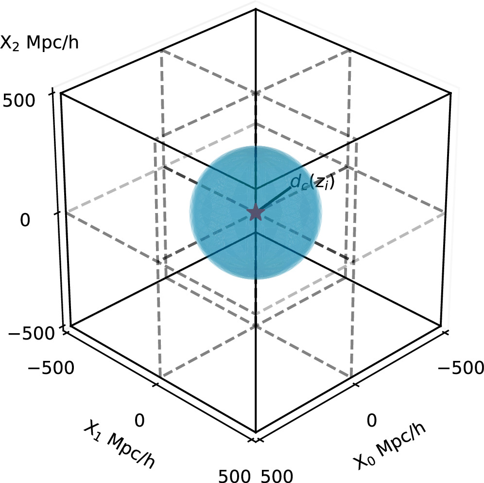
Figure 1. The new box, generated by replicating the initial simulation box eight times. The observer is positioned at the center, specifically at coordinates (0, 0, 0) Mpc h−1, with the surface of the past-lightcone at redshift z = zi presented for reference.
Download figure:
Standard image High-resolution imageA galaxy crosses the surface of the past-lightcone of the observer when its distance to the observer, given by  , matches the comoving distance that light can travel from z = 0 to the redshift of the target galaxy, denoted as dc(z). Since galaxies in the original catalog from the GABE–COSMIC methodology are stored in discrete snapshots, the galaxy, along with its associated GW events, is included in the mock lightcone catalog if it meets two criteria: (1) in the initial snapshot at zori, rori < dc(zori), and (2) in the subsequent snapshot at zdes, rdes > dc(zdes).
To determine the exact time t(zobs) of the galaxy as it crosses the surface of the past-lightcone between zori and zdes, two assumptions are employed: (1) the galaxy follows a straight-line trajectory between two adjacent snapshots,8 and (2) the comoving distance could be approximated to increase linearly with cosmic time t(z) during the interval. These assumptions yield the following two equations:

Consequently, t(zobs) corresponds to the time at which the two equations intersect, with the condition that at this intersection robs = dc(zobs). The position of the galaxy and the mean merger rates of merging stellar-mass compact binaries within the galaxy could be determined through linear interpolation:

where i = 0, 1, 2. The R.A. and decl. of the galaxy, which denote its directional orientation, are determined under the assumption that the coordinate system of the observer aligns with the equatorial coordinate system. By applying the aforementioned procedure to all galaxies with distances to the observer less than 250 Mpc h−1 in the original catalog from the GABE–COSMIC methodology, we construct the all-sky mock lightcone GW event catalog. We designate the all-sky mock lightcone GW event catalog, constructed with the observer positioned at coordinates (0, 0, 0) Mpc h−1 as described above, as the “r1” model. In addition to the r1 model, we change the observer’s location to generate six additional mock catalogs, labeled from “r2” to “r7” models. The coordinates of the observers for these models are detailed in Table 1. We select the r2 model as our fiducial model because it demonstrates the most significant anisotropy in the merging BBHs among the seven models (see results in Section 4.1).
Table 1. Observer Coordinates in the New Box for the Models “r2” Through “r7,” in Addition to the Observer Coordinate (0, 0, 0) Mpc h−1 for the Model “r1”
| Model | r2 | r3 | r4 |
|---|---|---|---|
| Pos/(Mpc h−1) | (125, 0, 0) | (250, 0, 0) | (250, 125, 0) |
| Model | r5 | r6 | r7 |
| Pos/(Mpc h−1) | (250, 250, 0) | (250, 250, 125) | (250, 250, 250) |
Download table as: ASCIITypeset image
The local merger rates from our seven catalogs are in good agreement with the results (436.8, 3.0, 37.0 Gpc−3 yr−1 for merging BNSs, NSBHs, and BBHs, respectively) from our previous work Z. Li et al. (2024), with differences within ∼30%. The local merger rates for BNSs and BBHs are also in strong agreement with the estimated local merger rates from GWTC-3 (R. Abbott et al. 2023b): 10–1700 Gpc−3 yr−1 for BNSs and 17.9–44 Gpc−3 yr−1 for BBHs. For NSBHs, the local merger rates in our study inherit the limitations from our previous work (Z. Li et al. 2024) and are lower than the estimated local merger rates from GWTC-3. A relevant discussion can be found in the second paragraph of Section 4.1 in Z. Li et al. (2024). However, using the overdensity to calculate the angular power spectrum would mitigate the underestimation. Furthermore, we did not observe any anomalous results for NSBHs when compared to BNSs and BBHs (see Section 4).
In principle, mock lightcone catalogs extending to higher redshifts could be constructed using a similar approach. However, due to computational limitations arising from the large number of galaxies and the associated merger rate information, our catalogs are restricted to z ∼ 0.085. Certain strategies could mitigate the computational burden, such as applying selection criteria to filter out less massive galaxies. For comparison, the mock lightcone catalog from J. Blaizot et al. (2005) used in A. C. Jenkins et al. (2018), which extends to z ∼ 0.78, contains only ∼42% of the number of galaxies compared with ours because its galaxies were selected based on an apparent AB magnitude cut of < 18 in the r filter from Sloan Digital Sky Survey (SDSS).
4. Results
4.1. The Angular Power Spectra
The HEALPix skymap of the overdensity δGW in the anisotropic SGWB from the merging BBHs up to dc = 250 Mpc h−1 at 60 Hz with Nside = 512 for the r2 model is shown in Figure 2. The overdensity distinctly traces the large-scale structure (LSS) of the universe, highlighting the filaments, nodes, and voids of the cosmic web. The skymaps for merging BNSs and NSBHs display similar characteristics, which are not presented here.
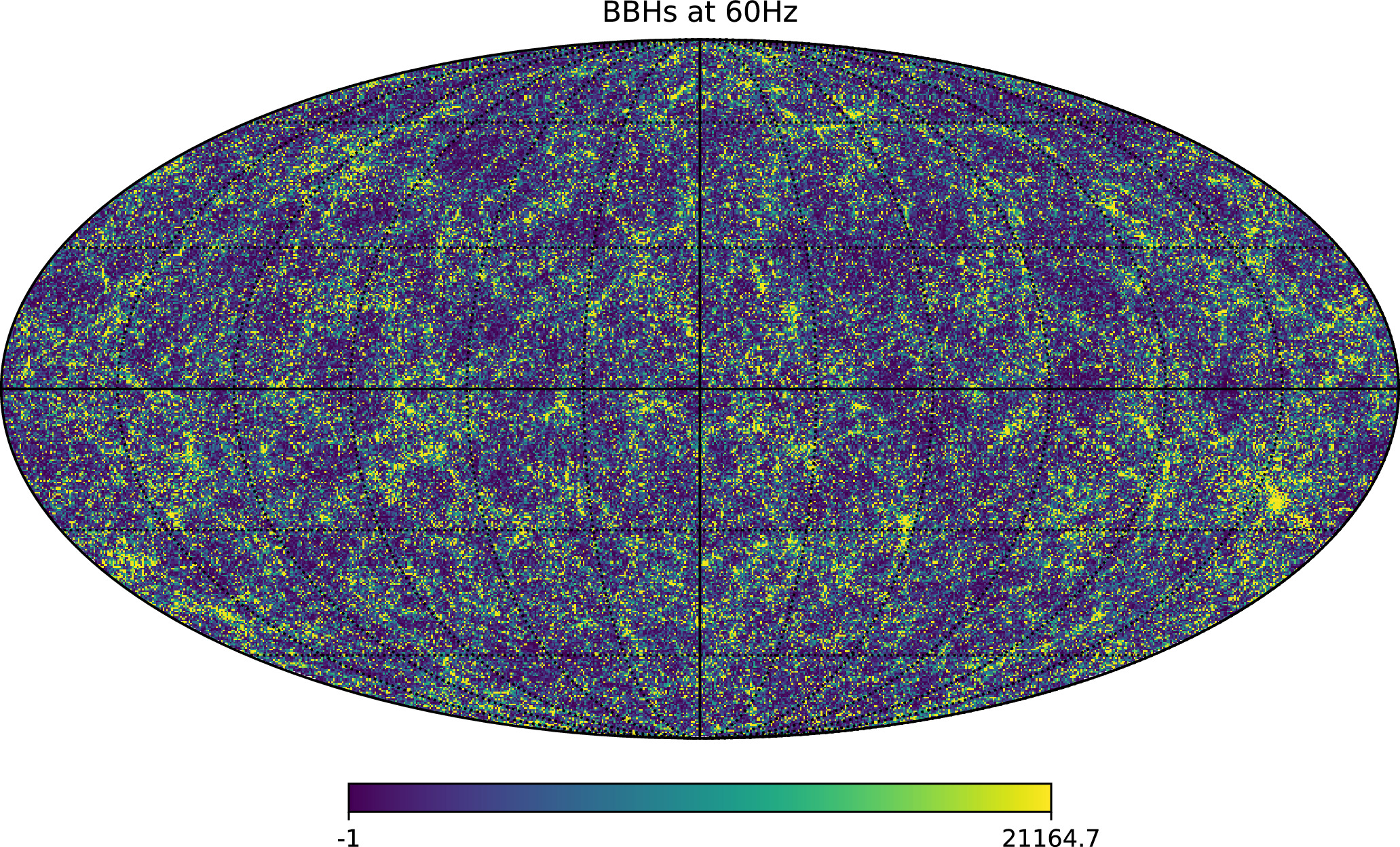
Figure 2. The HEALPix skymap of the overdensity δGW in the anisotropic SGWB from the merging BBHs up to dc = 250Mpc h−1 at 60 Hz with Nside = 512 for the r2 model.
Download figure:
Standard image High-resolution imageThe upper panel of Figure 3 presents the angular power spectra of the overdensity δGW in the SGWB from merging BNSs, NSBHs, and BBHs up to dc = 250 Mpc h−1 at 60 Hz, respectively, with Nside = 512, for the seven models, ranging from r1 to r7. All the spectra are contained within the colored regions, with the spectra for models r2 and r4 distinctly highlighted. The spectra for all three source types exhibit relatively flat shapes below ℓ ∼ 10, followed by steep upward trends. For higher ℓ (e.g., ℓ > ∼ 30–300), the trends are especially typical, with slopes β ≈ 2 in logarithmic space. The spectra across our seven catalogs exhibit considerable variations. For example, the spectra for merging BBHs exhibit a variation spanning approximately a factor of 2 to one order of magnitude for ℓ = 1 to ∼80 and about 1–2 orders of magnitude for ℓ = ∼ 80–1000. Our results are not directly comparable to those of A. C. Jenkins et al. (2018) and A. C. Jenkins et al. (2019a) for several reasons. First, the mock catalog used by A. C. Jenkins et al. (2018) extends to z ∼0.78, significantly surpassing the redshift range of the catalog in our study. Consequently, the spectra derived from closer sources may be higher, as discussed later. Additionally, their catalog includes only galaxies with apparent AB magnitudes limited to 18 in the r filter from SDSS, whereas our catalog encompasses all galaxies. However, we present a comparison here to highlight certain commonalities. Our spectra exhibit shapes similar to those reported by A. C. Jenkins et al. (2018) and A. C. Jenkins et al. (2019a) for higher ℓ (e.g., ℓ > ∼ 30–300). Their spectra for merging BBHs9 are generally situated near the lower boundary of the spectrum range for merging BBHs we obtained. We also conduct a brief comparison with the findings of G. Cusin et al. (2018), although our results are not directly comparable for several reasons. In addition to the limited redshift range explored in our study, differences in the GW energy spectrum and the models of merging stellar-mass compact binaries might also contribute to the disparity. The lower boundary of our spectra for merging BBHs exhibits significantly higher amplitudes (>2 orders of magnitude for the majority of ℓ) compared to the spectrum in G. Cusin et al. (2018).10

Figure 3. Upper panel: The angular power spectra of the overdensity δGW in the SGWB from merging BNSs, NSBHs, and BBHs up to dc = 250 Mpc h−1 at 60 Hz respectively, with Nside = 512, for the seven models, ranging from r1 to r7. All the spectra are contained within the colored regions, with the spectra for models r2 and r4 distinctly highlighted. Lower panel: Similar to the upper panel, but with nearby (<50 Mpc h−1) sources subtracted and exclusively highlights the spectra for the r2 model. The approximate scale of ℓ is indicated on the upper axis (rounded to one decimal place), along with reference lines (gray dashed lines) exhibiting slopes of β = 2 (note that the intercepts α are variable) in both panels.
Download figure:
Standard image High-resolution imageThe distribution of several nearby sources might contribute significantly to the fluctuations in anisotropy. To illustrate this effect, the angular power spectra of the overdensity δGW in the SGWB from merging BNSs, NSBHs, and BBHs between 50 and 250 Mpc h−1 at 60 Hz are shown, respectively, in the lower panel of Figure 3. After the subtraction of the nearby sources, the growth of the spectra relatively slows down within the range ∼10 < ℓ < ∼ 600, yet they continue to exhibit the typical sharp shapes for ℓ > ∼ 600. The variation in the spectra for the r1 to r7 models is significantly reduced across ℓ = 1–1000. The spectra for all three merging types exhibit a variation of less than a factor of ∼4 for ℓ = 1 to ∼20, and less than a factor of ∼2 for ℓ = ∼ 20–1000. The sharp reduction in variation after the subtraction indicates that the significant discrepancies observed in the spectra of the upper panel of Figure 3 are primarily attributable to the nearby sources. For each of seven mock catalogs, approximately 105 galaxies are situated within 50 Mpc h−1, accounting for roughly 0.5%–1% of the total galaxy population. However, the SGWB scales as  , as indicated by Equation (6). Consequently, nearer sources contribute more significantly to the SGWB. The variation regions of the spectra after the subtraction of nearby sources exhibit greater similarity to the error regions described in A. C. Jenkins et al. (2018) and A. C. Jenkins et al. (2019a) for higher ℓ (e.g., ℓ > ∼ 20). However, the shapes of the spectra more closely resemble the results reported by G. Cusin et al. (2018) within the range ∼10 < ℓ < ∼ 100. Note that to enable a more reasonable comparison with the existing literature in the future work, in addition to using a larger simulation box, several other factors should be addressed. For example, when comparing with A. C. Jenkins et al. (2019a), it is essential to apply a magnitude filter to our galaxy catalogs. Furthermore, understanding the influence of the GW energy spectra and the models of merging stellar-mass compact binaries on anisotropy is essential for comparisons with G. Cusin et al. (2018).
From the observational perspective, the contribution to the total SGWB from nearby sources would be the first to be subtracted by future GW detectors because these discrete events are the most readily detectable. As more nearby sources are resolved with accurate positional information, the significant uncertainty in the theoretically predicted angular power spectra of the overdensity in the SGWB, arising from the mapping of these sources onto the skymap, will progressively decrease. Ultimately, the theoretical angular power spectra for the residual SGWB will exhibit a much narrower uncertainty range, as shown in the lower panel of Figure 3. Consequently, these spectra will be better suited for comparison with other theoretical predictions or future observational results, enabling the potential extraction of astrophysical (or cosmological) information, such as LSS. Subtracting nearby sources would also mitigate the necessity for highly accurate mock GW event catalogs in predicting the angular power spectra. After the subtraction of the nearby sources, the spectra for merging BNSs, NSBHs, and BBHs at 60 Hz display notable similarities (within discrepancies of a factor of ∼2 across ℓ = 1–1000 for all catalogs). This result suggests that the anisotropy is primarily influenced by the distribution of GW source hosts and might serve as a valuable probe of the LSS of the universe. Typically, anisotropy from CBCs can also be investigated through directly detected GW sources, as demonstrated in E. Payne et al. (2020). However, studies of the SGWB offer complementary methods. In this study, our spectra establish a theoretical upper limit11 on the anisotropy from CBCs. The spectra might also be compared with other angular power spectra defined by overdensity, such as the CMB spectra, in the future, potentially uncovering additional and deeper astrophysical and cosmological insights, such as those related to matter distribution and galaxy clusters. Additionally, an accurate angular power spectrum for the SGWB from astrophysical GW sources in the future could establish a limit for the detectable anisotropy of the SGWB originating from potential cosmological GW sources that cannot be individually detected, such as cosmic strings (e.g., A. C. Jenkins & M. Sakellariadou 2018). Below this limit, these SGWB components might be masked.
4.2. The Effects of the Radial Distribution
The spatial distribution of the sources could be decomposed into two parts: the angular distribution on the celestial sphere, referred to as “azimuthal distribution,” and the distribution at different comoving distances, referred to as “radial distribution.” The influence of the radial distribution on the anisotropy is assessed through the implementation of the following smoothing process in our work. We partition the comoving distances of galaxies, along with the merging stellar-mass compact binaries they contain, into m equally spaced bins within the range [a, b] Mpc/h, referred to as “m-bin approximation.” Here, a and b denote the lower and upper boundaries of the comoving distances of the considered sources, respectively. For example, in the 5-bin approximation, the bin boundaries are defined as [a,  ,
,  ,
,  ,
,  , b] Mpc h−1. The comoving distances of the galaxies within each bin, denoted as dc,i,1, dc,i,2...
  are then replaced by the mean comoving distance for that bin, given by
  , where i represents the bin index and ni is the total number of the galaxies within the bin. The variation in the spectra between those calculated directly and those obtained using the m-bin approximation is interpreted as the anisotropy potentially influenced by the radial distribution. We anticipate that the extreme case of m = 1, corresponding to the 1-bin approximation, captures the anisotropy approximately arising from the azimuthal distribution. In this work, we use the approximation model to study sources up to dc = 50 Mpc h−1 (a = 0, b = 50), between 50–250 Mpc h−1 (a = 50, b = 250), and up to dc = 250 Mpc h−1 (a = 0, b = 250).
To evaluate the impact of the radial distribution of both nearby and farther sources on the anisotropy, we calculate the angular power spectra of the overdensity δGW in the SGWB from merging BBHs up to dc = 50 Mpc h−1 and between 50–250 Mpc h−1, derived from direct calculation, the 5-bin approximation model, and the 1-bin approximation model, respectively, with Nside = 512 at 60 Hz in the r2 model. The results are presented in the upper panel of Figure 4. The colored regions illustrate the influence of the radial distribution. The variation of the spectra for the sources within dc = 50 Mpc h−1 is within a factor of ∼3 for ℓ = 1 to ∼10, a factor of ∼2 to approximately one order of magnitude for ℓ = ∼ 10 to ∼50, and ∼1–2 orders of magnitude for ℓ = ∼ 50–1000. For the sources situated between 50–250 Mpc h−1, the variation is within a factor of ∼3 for ℓ = 1 to ∼10, and within about 30% for ℓ = ∼ 10–1000. Consequently, when modeling the anisotropy with the subtraction of nearby sources, the radial distribution of sources becomes less significant for higher ℓ (e.g., ℓ > ∼ 10). The directly calculated spectrum for sources up to dc = 50 Mpc h−1 exhibits the typical upward shape for ℓ > ∼ 30, as shown by the “BBHs r2” spectrum in the upper panel of Figure 3. However, the directly calculated spectrum for sources within the range of 50–250 Mpc h−1 does not display this shape until ℓ > ∼ 600, as shown by the spectra in the lower panel of Figure 3. Since observational factors are not incorporated in our analysis, the angular power spectra presented in our current work do not include instrumental noise. For further discussion on the angular power spectrum of the instrumental noise, see D. Alonso et al. (2020a).

Figure 4. Upper panel: The angular power spectra of the overdensity δGW in the SGWB from merging BBHs within dc = 50 Mpc h−1 and between dc = 50–250 Mpc h−1, derived from direct calculation, the 5-bin approximation model, and the 1-bin approximation model, respectively, with Nside = 512 at 60 Hz in the r2 model. The colored regions illustrate the influence of the radial distribution. Lower panel: The angular power spectra of the overdensity δGW in the SGWB from merging BBHs up to dc = 250 Mpc h−1 at 60 Hz, derived from the 5-bin approximation model, with Nside = 512, for the seven models, ranging from r1 to r7. All the spectra are contained within the colored regions, with the spectrum for the r2 model distinctly highlighted. The approximate scale of ℓ is indicated on the upper axis (rounded to one decimal place), along with reference lines (gray dashed lines) exhibiting slopes of β = 2.
Download figure:
Standard image High-resolution imageThe lower panel of Figure 4 shows the angular power spectra of the overdensity δGW in the SGWB from merging BBHs up to dc = 250 Mpc h−1 at 60 Hz, derived from the 5-bin approximation, with Nside = 512, for the seven models, ranging from r1 to r7. All the spectra are contained within the blue regions, with the spectrum for the r2 model distinctly highlighted. The spectra exhibit minimal variation (less than a factor of ∼3.5) across our seven mock catalogs for ℓ > ∼ 10. This observation also suggests that the significant variation in the spectra presented in the upper panel of Figure 3 for ℓ > ∼ 30 might primarily arise from fluctuations in the radial distribution of the nearby sources. The discrete nature of the processes underlying the SGWB, such as the discrete spatial and temporal distribution of GW sources, often leads to Poisson noise, also known as shot noise (see A. C. Jenkins & M. Sakellariadou 2019; A. C. Jenkins et al. 2019b; D. Alonso et al. 2020b; N. Kouvatsos et al. 2024 for further discussion). The fluctuations in the radial distribution in our analysis might mainly result from inherent Poisson noise in our catalogs, arising from the discreteness of galaxies (and the GW sources within them) in the radial distribution. The primary term contributing to the radial dependence in Equation (6),  , originates from the calculation of the comoving number density
  in Equation (5). Consequently, the radial distribution of sources represents the number density of galaxies within each comoving volume element dVc,e at various redshifts, which inherently includes Poisson noise. When the number of galaxies is small (e.g., ∼105 within 50 Mpc h−1 in our models), this noise might predominate in the estimation of the anisotropic SGWB.
We note that the spectra for both merging BBHs up to dc = 50 Mpc h−1 and between 50 and 250 Mpc h−1 exhibit typical shapes for higher ℓ (e.g., ℓ > ∼ 300–600), even under the extreme 1-bin approximation. Consequently, other factors might contribute to the Poisson noise. The typical shapes of our spectra exhibit slopes similar to those of the modeled Poisson noise spectra presented in G. Cusin et al. (2019). Additionally, the spectral behavior aligns with the predictions made in G. Cusin et al. (2019), which suggest that the high ℓ (e.g., ℓ > ∼ 50 to ∼600, based on the different choice of integral cut-off, shown in their Figure 9) portion of the angular power spectrum is predominantly influenced by Poisson noise arising from the azimuthal distribution of mock catalogs. This might indicate that the Poisson noise from the azimuthal distribution is entangled within our spectra. In addition to Poisson noise, cosmic variance, arising from the variation in observer positions across our seven models, might also contribute to the fluctuations in the galaxy distributions within our catalogs. This might account for some of the variation in the angular power spectra across our seven models, particularly at lower values of ℓ (e.g., ℓ < ∼ 10). However, it is unlikely to be the primary factor directly contributing to the observed large variation of the angular power spectra for ℓ > ∼ 10 in the upper panels of Figures 3 and 4 because it primarily affects the angular power spectra at lower ℓ (e.g., ℓ < ∼ 10) and has minimal impact for higher ℓ (e.g., ℓ > ∼ 10), as shown in Figure 4 of A. C. Jenkins et al. (2018). Nevertheless, cosmic variance could have an indirectly profound impact on the angular power spectra because it reflects underlying variations in the distribution and number density of galaxies, which in turn influence the Poisson noise. For instance, in more densely populated regions of the universe, relative Poisson noise might be smaller, while in more sparsely populated regions, it might be larger.
4.3. The Effects of Including Farther Sources
Figure 5 presents the ratio of the angular power spectra of the overdensity δGW in the SGWB from merging BBHs up to various comoving distances, relative to the angular power spectrum of the overdensity δGW in the SGWB from merging BBHs up to 50 Mpc h−1, at 60 Hz with Nside = 512 in the r2 model. As sources at higher redshifts are included, the ratio decreases across ℓ = 1–1000. For instance, the contribution from sources beyond 100 Mpc h−1 to the total anisotropy is expected to be less than ∼30%–40%. Meanwhile, the rate of decrease seems to slow. In comparison to the spectrum that incorporates sources up to 100 Mpc h−1 (Cℓ,100Mpc/h), the spectrum that includes sources up to 150 Mpc h−1 (Cℓ,150Mpc/h) shows a reduction of approximately 1.7–2.5 times across the range ℓ = 1–1000. However, when comparing the spectrum with sources up to 200 Mpc h−1 (Cℓ,200Mpc/h) to that with sources up to 250 Mpc h−1 (Cℓ,250Mpc/h), the latter exhibits a decrease of roughly 1.3–1.6 times across the range ℓ = 1–1000. Although a larger simulation box is necessary for a comprehensive exploration of the universe, our findings establish an upper limit for the anisotropy.

Figure 5. The ratio of the angular power spectra of the overdensity δGW in the SGWB from merging BBHs up to various comoving distances, relative to the angular power spectrum of the overdensity δGW in the SGWB from merging BBHs up to 50 Mpc h−1, at 60 Hz with Nside = 512 in the r2 model. The approximate scale of ℓ is indicated on the upper axis (rounded to one decimal place).
Download figure:
Standard image High-resolution image5. Summary and Discussion
Anisotropic SGWB could serve as a probe of the spatial distribution of GW sources. We explore the anisotropic SGWB from local merging BBHs, NSBHs, and BNSs (dc < 250 Mpc h−1) by constructing seven all-sky mock lightcone GW event catalogs. The HEALPix skymaps of the overdensity δGW in the anisotropic SGWB were generated using these mock catalogs. The HEALPix skymap of the r2 model for merging BBHs shown in Figure 2 serves as an example to illustrate the anisotropic distribution of the GW sources.
Based on the HEALPix skymaps, the angular power spectra in terms of log10[ℓ(ℓ + 1)Cℓ/(2π)] are calculated to quantify the anisotropy level of the SGWB from merging stellar-mass compact binaries. As shown in the upper panel of Figure 3, the spectra for all three source types exhibit a typical shape at higher ℓ (e.g., ℓ > ∼ 30–300) across all catalogs, featuring an approximately linear increase with log10ℓ: log10[ℓ(ℓ + 1)Cℓ/(2π)] ∝ β(log10ℓ), with a characteristic slope of β ∼ 2. The spectra for our seven catalogs exhibit considerable variations. For example, the spectra for merging BBHs in different catalogs vary by approximately a factor of 2 to one order of magnitude for ℓ = 1 to ∼80, and by about 1–2 orders of magnitude for ℓ = ∼ 80–1000. The fluctuation in the distribution of the nearby (e.g., <50 Mpc h−1) sources should contribute to the variations of the spectra for merging BBHs, NSBHs, and BNSs. Subtracting these nearby sources results in significant reductions of the variations of the spectra. Shown in the lower panel of Figure 3, after the subtraction of the nearby sources, all spectra vary within a factor of ∼4 for ℓ = 1 to ∼20, and within a factor of ∼2 for ℓ = ∼ 20 to 1000. The spectra for the three source types then become closely aligned (within discrepancies of a factor of ∼2 across ℓ = 1–1000 for all catalogs). This result indicates that the SGWB anisotropy is primarily influenced by the distribution of the hosts of GW sources and could be used as a probe of the LSS of the universe.
We further examine the contribution of the radial distribution of GW sources to the anisotropy of the SGWB. The results for merging BBHs are shown in Figure 4. The random distance of the nearby sources makes the main contribution to the anisotropy of the SGWB (the red region in the upper panel of Figure 4). After the subtraction of the nearby sources, the radial distribution has an insignificant effect on the spectra (implied by the green region in the upper panel of Figure 4), and the anisotropy from the azimuthal distribution (approximately estimated using the 5-bin approximation) of sources varies within ∼3.5 times across our seven mock catalogs (the blue region in the lower panel of Figure 4), for ℓ > ∼10. Therefore, the considerable spectral variations for ℓ > ∼ 30 shown in the upper panel of the Figure 3 could be attributed to the radial distribution of the nearby sources. This random radial distribution of nearby sources might be the main Poisson noise, and contributes to the typical spectral shape as shown in G. Cusin et al. (2019). However, even with the extreme 1-bin approximation, namely the anisotropy approximately originating from the azimuthal distribution, the spectra continue to exhibit typical shapes for higher ℓ (e.g., ℓ > ∼ 300–600). This indicates that the variation of spectra for the seven mock catalogs also include the Poisson noises from the azimuthal distribution. We also find that including farther sources results in a rapid decrease in the anisotropy in Figure 5. However, the rates of decrease seem to diminish as sources at higher z are included.
Besides the above results from the spectra for the merging BBHs shown in Figures 4 and 5, similar conclusions could also be obtained for both merging NSBHs and BNSs results. Furthermore, we investigate the effects of the observation frequency and the angular resolution of skymap on the spectra. We find that during the most sensitive observation frequency for LIGO, ranging from about 20 to 100 Hz, the spectra exhibit negligible variation. The spectra calculated from the HEALPix skymaps at different resolutions, specifically with Nside = 32, 64, 128, 256, 512, are also consistent across the various configurations.
Acknowledgments
We acknowledge valuable input from our anonymous referee. This work has been supported by the National Natural Science Foundation of China (Nos. 11988101, 11922303, 12033008, and 11673031), the K.C. Wong Education Foundation, and the National Key Research and Development Program of China (grant Nos. 2020YFC2201400, SQ2021YFC220045-03). We acknowledge the use of the healpy and HEALPix packages in deriving the results presented in this paper.
Software: healpy (A. Zonca et al. 2019); HEALPix (K. M. Górski et al. 2005); GABE (Z. Jiang et al. 2019); COSMIC v3.3.0 (K. Breivik et al. 2020a, 2020b); NumPy (C. R. Harris et al. 2020); Matplotlib (J. D. Hunter 2007); Astropy (The Astropy Collaboration et al. 2013, 2018, 2022); SciPy (P. Virtanen et al. 2020); Numba (S. K. Lam et al. 2015); Jupyter (T. Kluyver et al. 2016); Python (https://www.python.org).
Footnotes
- 6
- 7
- 8
This assumption is widely used (e.g., J. Blaizot et al. 2005; M. G. Kitzbichler & S. D. M. White 2007; A. I. Merson et al. 2013; D. Korytov et al. 2019). Different interpolation methods for galaxy positions between snapshots show nearly identical precision, with small differences (e.g., ∼10−2 Mpc h−1), as detailed in A. Smith et al. (2022), that are negligible for our analysis.
- 9
The spectrum reported by A. C. Jenkins et al. (2018) includes all three types of merging stellar-mass compact binaries but introduces only a
 difference, as noted by the authors.
 - 10
- 11
Our analysis considers sources within the distance of 250 Mpc h−1. Incorporating more distant sources would reduce the anisotropy, as further discussed in Section 4.3.
