Abstract
Probing the speed of light is an important test of general relativity, but the measurements of c using objects in the distant universe have been almost completely unexplored. In this paper, we propose an idea to use the multiple measurements of galactic-scale strong gravitational lensing systems with Type Ia supernovae acting as background sources to estimate the speed of light. This provides an original method to measure the speed of light using objects located at different redshifts that emitted their light in a distant past. Moreover, we predict that strongly lensed Type Ia supernovae observed by the Large Synoptic Survey Telescope (LSST) would produce robust constraints on Δc/c at the level of 10−3. We also discuss whether future surveys such as LSST may succeed in detecting any hypothetical variation of c predicted by theories in which fundamental constants have a dynamical nature.
1. Introduction
As one of the cornerstones of general relativity, as well as of many other gravitational theories, the speed of light c plays a very important role in modern physics. On the other hand, during the past 2 decades great attention has been paid to the theories with varying speed of light (VSL), in which the speed of light might be dynamical and could have been varying in the past. Any possible violation of constancy of c would have far-reaching consequences for our understanding of nature. The interest in VSL theories was triggered by the conjecture that they could become an alternative to the inflationary mechanism of solving standard cosmological problems (Albrecht & Magueijo 1999; Barrow 1999; Barrow & Magueijo 1999). On the tide of growing popularity of VSL approach, Davies et al. (2002) claimed that variation of the speed of light can be discriminated from variation of the elementary charge based on the entropy of black holes. Later this claim was refuted by Carlip & Vaidya (2003) and Flambaum (2002). It is worth recalling that Ellis & Uzan (2005) gave a sobering review of serious conceptual problems one faces while trying to change the status of c in physics. In particular, they stressed that it is usually not consistent to allow a constant to vary in an equation that has been derived from a variational principle under the hypothesis of this quantity being constant. Therefore, one needs to go back to the Lagrangian and derive new equations after having replaced the constant by a dynamical field.
Although c has been measured with a very high precision, most of these measurements were carried out on Earth or in our close cosmic surroundings. Recently, however, some advances have been made concerning measurements of the speed of light using extragalactic objects. Considering the relation between the maximum value of the angular diameter distance DA(z) and the Hubble parameter H(z) corresponding to this maximum, Salzano et al. (2015) discussed (on the simulated data) the possibility of using the baryon acoustic oscillations (BAOs) to place constraints on the variation of the speed of light. Then, Cai et al. (2016) investigated the constancy of c using independent observations of Hubble parameters H(z) and luminosity distances from Type Ia supernovae (SNe Ia) (Suzuki et al. 2012). The measurement of c in the distant universe is an almost completely uncharted territory. Recently, with the angular diameter distances measured for intermediate-luminosity quasars extending to high redshifts, Cao et al. (2017a) performed the first measurement of the speed of light referring to the redshift baseline z = 1.70. The result was in very good agreement with the value of c obtained on Earth (i.e., at z = 0).
Gravitational lensing creates another opportunity to test the speed of light. In the well-known gravitational lens Q0957+561 (Walsh et al. 1979; Young et al. 1981), the appearance of two images of a zs = 1.41 quasar within an Einstein radius of 308 around the core of the lensing galaxy at zl = 0.36 has opened up a wide range of possibilities of using strong-lensing systems in cosmology and astrophysics (Grillo et al. 2008; Biesiada et al. 2010; Cao & Zhu 2012, 2014; Cao et al. 2012, 2012, 2013, 2015, 2016a, 2017c; Li et al. 2016). Strongly lensed SNe Ia, which have long been predicted in the literature (Refsdal 1964), remained undiscovered until very recently. Eventually, Goobar et al. (2017) reported the discovery of a new gravitationally lensed SN Ia, iPTF16geu (SN 2016geu), from the intermediate Palomar Transient Factory (iPTF). Strong-lensing time-delay predictions for this system were discussed in detail in More et al. (2017).
Here, we will focus on the idea of constraining c by using the measurements of galactic-scale strong gravitational lensing systems with SNe Ia acting as background sources. In a specific strong-lensing system, time delay between the images of strongly lensed SNe Ia is directly related to the speed of light, the Fermat potential difference, and the so-called time-delay distance. This opens a possibility to measure the speed of light on the baseline up to the redshift of the source.
2. Methodology
General relativity predicts that light can be deflected by massive objects (e.g., galaxies), resulting in distorted multiple images of the background sources. For a specific strong-lensing system with the lensing galaxy at redshift zl, the multiple-image separation of the source at redshift zs depends on the ratio of angular diameter distances between lens and source Dls and between observer and source Ds (Schneider et al. 1992). In a spatially flat Friedman–Lemaître–Robertson–Walker metric the formula for the angular diameter distance reads

where H0 is the Hubble constant and E(z) is the dimensionless expansion rate dependent on redshift z. It should be stressed at this point that even though we mentioned VSL theories above, we do not make use of any of these models. On the contrary, we use (here and in the equations that follow) the standard theory perceiving our goal as a measurement of the speed of light using extragalactic objects. We use the expression  instead of just c in order to emphasize that the speed of light would be determined on the baseline between the observer z = 0 and the source zs. Hence, if the measured value turns out to be
  within statistical and systematic uncertainties, this would be a confirmation of the constancy of c (and hence the standard physics that we know on Earth) using very distant objects. On the contrary, if
  significantly (note that this may happen in a space-dependent manner), this could be a signal that c was not a fundamental constant, triggering further theoretical work in order to explain this result. Last but not least, our approach makes it clear that, although we report dimension-full
  , we do really constrain the dimensionless ratio
  or Δc/c.
Provided that the background source is an SN Ia that is a transient event with a well-defined light curve after peak, the strong-lensing time-delay effect due to different light paths combined with the Shapiro effect will be revealed in the photometry of its multiple images. Recently, strong gravitational time delays between the multiple images have become a promising tool in cosmology providing alternative measurements of the Hubble constant (Suyu et al. 2017; Liao et al. 2017). According to the theory of gravitational lensing, time delay between images  and
and  can be written as (Treu 2010)
where ![${\rm{\Delta }}{\phi }_{i,j}=[{({{\boldsymbol{\theta }}}_{i}-{\boldsymbol{\beta }})}^{2}/2-\psi {({{\boldsymbol{\theta }}}_{i})-({{\boldsymbol{\theta }}}_{j}-{\boldsymbol{\beta }})}^{2}/2+\psi ({{\boldsymbol{\theta }}}_{j})]$](https://content.cld.iop.org/journals/0004-637X/867/1/50/revision1/apjaae5f7ieqn8.gif) is the Fermat potential difference determined by the lens mass distribution. The source position, with respect to the line connecting the observer and the center of the lens, is denoted by
is the Fermat potential difference determined by the lens mass distribution. The source position, with respect to the line connecting the observer and the center of the lens, is denoted by  , and ψ denotes the 2D lensing potential fulfilling the Poisson equation ∇2ψ = 2κ, where κ is dimensionless surface mass density (convergence) of the lens. The time-delay distance is defined as

where Dls and Ds are angular diameter distances between the lens and the source and between the observer and the source, respectively.
Assuming a flat Friedman–Robertson–Walker metric, one can relate the angular diameter distance DA to the proper distance DP according to  . Since proper distances are additive, the distance ratio of
  can be expressed in terms of angular diameter distances Dl and Ds,

By combining Equations (1)–(4), one can express the speed of light as
which suggests how to measure this quantity using strong-lensing systems. Note that for each specific strong-lensing system, the derivation of Equations (2)–(5) is based on the choice that  denotes the constant speed of light related to the baseline from the source to the observer. It is also straightforward to check that when the speed of light is a function of redshifts, the accurate derivation of the above equations could be very different, since the cosmological distances contain an extra factor c(z) outside the integral (Qi et al. 2014).
Current observational techniques allow the redshifts of the lens zl and the source zs to be measured precisely. Moreover, imaging and spectroscopy from the Hubble Space Telescope (HST) and ground-based observatories make it possible to derive three key ingredients for individual lenses: stellar velocity dispersion, high-resolution images of the lensing systems, and time delays. On the one hand, current high-resolution image astrometry, combined with the state-of-the-art lens modeling techniques (Suyu et al. 2010, 2012) and kinematic modeling methods (Auger et al. 2010; Sonnenfeld et al. 2012), will precisely determine the multiple image positions of the background source and the Einstein radius of the lensing system and thus place stringent limits on the Fermat potential  with <3% uncertainty (including the systematics; Suyu et al. 2013, 2014; Liao et al. 2015). In practice, we also need to quantify the influence of matter along the line of sight (LOS) on the lens potential, contributing an extra systematic uncertainty at the 1% level (Suyu et al. 2017). On the other hand, in the framework of typical quasar–elliptical galaxy lensing systems, well-measured light curves combined with new curve shifting algorithms (Tewes et al. 2013a) could provide
  measurements typically with 3% accuracy (Fassnacht et al. 2002; Courbin et al. 2011; Tewes et al. 2013b; Dobler et al. 2015; Liao et al. 2015). Time delays measured in lensed SNe Ia are supposed to be very accurate owing to exceptionally well characterized spectral sequences and considerable variation in light-curve morphology (Nugent et al. 2002; Pereira et al. 2013). In this analysis, in the framework of SN Ia–elliptical galaxy lensing systems, the fractional uncertainty of Δt is taken at the level of 1%, which is a reasonable assumption for well-measured light curves of lensed SNe Ia.
Concerning the time-delay distance, one might be tempted to pre-assume the cosmological model, e.g., as a flat ΛCDM with  , but this would introduce a hardly controllable bias. A more reasonable approach is to derive the distances to the lens and to the source based on their redshifts and using the absolute distances to standard candles at these redshifts. It is commonly believed that unlensed SNe Ia can be calibrated as standard candles, which, combined with the so-called distance–duality relation (Etherington 1933; Cao & Liang 2011; Cao et al. 2016b), can provide the DA(z) (in units of Mpc) at both lens and source redshifts:
where mX is the peak apparent magnitude of the SN in filter X, MB is its rest-frame B-band absolute magnitude, and KBX denotes the cross-filter K-correction (Kim et al. 1996). For the purpose of our analysis, we determined the angular diameter distances Dl and Ds of strongly lensed SNe Ia by fitting a polynomial to the unlensed SN Ia data. Therefore, we bypassed the need to pre-assume any specific cosmological model. We expect that, in the near future, much bigger depth, area, resolution, and sample sizes brought by the next-generation wide and deep sky surveys (Marshall et al. 2005) will yield a huge number of strong-lensing systems discovered, including lensed SNe Ia. In the following, we will illustrate what kind of results one could get using the future data from the forthcoming Large Synoptic Survey Telescope (LSST).
3. Simulated Data
Within the next decade new wide-area imaging surveys are likely to discover thousands of lensed SNe Ia, time-delay measurements of which will be derived from their time-domain information (observed by repeated scans of sky) and dedicated follow-up monitoring campaigns. Detailed calculation of the likely yields of several planned strong-lensing surveys was recently performed by Goldstein & Nugent (2017). Considering realistic simulation of lenses and sources, they found that LSST can discover up to 500 multiply imaged SNe Ia in a 10 yr z-band search, which is an improvement of more than an order of magnitude over previous estimates (Oguri & Marshall 2010), while the LSST is expected to yield 106 unlensed SNe Ia (Cullan et al. 2017).
In the framework of the method proposed by Collett (2015), we first simulated a population of realistic strong lenses possible to be observed by LSST. Because elliptical galaxies dominate in the galaxy lensing cross section (Oguri & Marshall 2010), we considered only SNe Ia lensed by early-type galaxies, whole velocity dispersion function in the local universe follows the modified Schechter function (Choi et al. 2007; for discussion about such a choice in view of other data on velocity dispersion distribution functions, see Cao & Zhu 2012; Biesiada et al. 2014). In order to assess the accuracy of the Fermat potential recovery, we assumed the elliptically symmetric power-law lens model, which has been widely used in several studies of X-ray observations of galaxies (Humphrey & Buote 2010), as well as strong lensing caused by early-type galaxies (Koopmans et al. 2006, 2009; Treu et al. 2006; Gavazzi et al. 2007). Following previous works (Oguri et al. 2008; Oguri & Marshall 2010), we assumed a Gaussian distribution for the ellipticity  . Meanwhile, lens velocity dispersions are directly related to their masses. So, in order to check how well our simulation represents real lenses, we found that our simulated population of lenses is dominated by galaxies with
  km s−1, having approximately Gaussian distribution characterized by σv = 210 ± 50 km s−1. These parameters could be inferred from high-quality imaging observations through state-of-the-art lens modeling techniques (Suyu et al. 2010, 2012) and kinematic modeling methods (Auger et al. 2010; Sonnenfeld et al. 2012). Comparison of this result with the SL2S sample, concerning the distribution of the velocity dispersion in the population of lenses, reveals similarity between the simulations and the real observations (Sonnenfeld et al. 2013).
In order to produce a catalog of lensed SN Ia candidates, three sources of uncertainties are included in our simulation of lensed SNe Ia: time delay, Fermat potential difference, and the LOS effect (Liao et al. 2017). First, compared with strongly lensed galaxies and quasars, which have already been discovered in large number (Cao et al. 2015; Shu et al. 2017), strongly lensed SNe Ia have notable advantages over traditional strong lenses as time-delay indicators. More specifically, benefiting from exceptionally well characterized spectral sequences and relatively small variation in quickly evolving light-curve shapes and color (Nugent et al. 2002; Pereira et al. 2013), time delays measured from lensed SNe Ia are less onerous than from active galactic nuclei and quasars. Therefore, as pointed out in the recent analysis by the strong-lens time-delay challenge (Dobler et al. 2015; Liao et al. 2015), the fractional uncertainty at the level of 1% can be achieved for  . Second, a high-resolution imaging while the SNe Ia are still active is necessary to precisely determine the lens potential. Our simulation of a system with the lensed SN Ia image quality typical of the HST observations and recovery of the relevant parameters with state-of-the-art lens modeling techniques demonstrates that one can achieve the lens modeling (i.e., the Fermat potential difference) precision at ∼3% level for a single well-measured time-delay lens system (Suyu et al. 2017). Finally, despite these advantages, lensed SNe Ia still face the problem of the LOS contamination. Using the technique of simulations of many multiple-image configurations, one could be able to quantify the influence of the matter along the LOS on strong-lensing systems (Jaroszyński & Kostrzewa-Rutkowska 2012). Further progress in this direction has been achieved by Collett et al. (2013), with the publicly available code Pangloss reconstructing the mass along a line of sight up to intermediate redshifts. We assumed that the LOS contamination might introduce 1% uncertainty in the lens potential (Liao et al. 2017).
We performed a Monte Carlo simulation to create the unlensed SN Ia sample. The simulation was carried out in the following way: (1) When calculating the sampling distribution (number density) of the SN Ia population, we adopted the redshift-dependent SN Ia rate from Sullivan et al. (2000). In each simulation, there were 5000 SNe Ia covering the redshift range of 0.00 < z ≤ 1.70. (2) Following the suggestion of Goldstein & Nugent (2017), the peak rest-frame MB was assumed normally distributed with a mean of −19.3 and standard deviation of 0.2, while the cross-filter K-corrections were computed from the one-component SN Ia spectral template of Nugent et al. (2002; see Barbary 2014 for more details). (3) Three sources of uncertainties were included in the peak apparent magnitude of the SN. First, following the strategy described by the WFIRST Science Definition Team (Spergel et al. 2015), the distance precision per SNe was determined by the following uncertainty model:  (Hounsell et al. 2017), with the mean uncertainty (including both statistical measurement uncertainty and statistical model uncertainty) σmeas = 0.08 mag, the intrinsic scatter uncertainty σint = 0.09 mag, and the lensing uncertainty set to be σlens = 0.07 × z mag (Holz & Hughes 2005; Jönsson et al. 2010). Moreover, the total systematic uncertainty was also considered in the corrected SN Ia distances, which is modeled as
  (Hounsell et al. 2017).
In Table 1 we list the relative or absolute uncertainties of the above-mentioned factors contributing to the accuracy of c measurement. Assuming that parameters whose uncertainties listed in Table 1 follow Gaussian distributions, one is able to obtain c and its average value using Equation (5). In order to guarantee unbiased final results, this process was repeated 103 times for each strong-lensing system.
Table 1. Relative Uncertainties of Factors Contributing to the Accuracy of c Measurement
| δΔt | δΔψ | δ LOS | ||
|---|---|---|---|---|
| Lensed SNe Ia | 1% | 3% | 1% | |

|

|

|

|
|
| Unlensed SNe Ia | 0.08 | 0.09 | 0.07 × z | 0.01(1 + z)/1.8 |
Note. δΔt, δΔψ, and δ LOS correspond to time delay, fermat potential difference, and light-of-sight contamination, respectively. The second row displays different factors contributing to the uncertainty of the magnitude of unlensed SNe Ia. σmeas, σint, σlens, and σsys denote the photometric measurement uncertainty, the intrinsic scatter, the lensing magnification uncertainty, and the total systematic uncertainty, respectively.
Download table as: ASCIITypeset image
4. Results and Discussion
Expected results of the speed-of-light measurements obtained from LSST are shown in Figure 1. Previous successful measurement of c using the quasar sample combined with the expansion rate function H(z) based on the data from cosmic chronometers and BAOs (see Qi et al. 2018 for the recent observations of Hubble parameters), even though being an important achievement providing the first assessment of the speed of light referring to the distant past, was just a single measurement with the baseline z = 1.70 (Cao et al. 2017a). In contrast, concerning the method proposed here, we expect that the high-resolution imaging of LSST will make it possible to discover a large number of strong-lensing systems leading to N ∼ 500 measurements of c for the optimal imaging case. The question now arises, Are these measurements sufficient enough to detect possible VSL effects? Considering the high-precision measurement of the speed of light c0 on Earth, with the fractional uncertainty of 10−9, it is very difficult to achieve competitive results with cosmological measurements. SN Ia observations, however, would provide us with the value of  , the speed of light at redshift baseline zs, from which we may study the accuracy concerning the deviation from c0,
  . The effectiveness of our method could be seen from the precision of measurements of c at different redshift baselines. These are summarized in Figures 2 and 3. The forecast for the LSST survey is as follows: strongly lensed SNe Ia observed by LSST would produce robust constraints on the speed of light at the level of
  , if the distance measurements from unlensed counterparts are available. This is the most unambiguous result of the current data set.
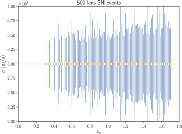
Figure 1. Individual measurements of the speed of light from the forthcoming LSST survey.
Download figure:
Standard image High-resolution image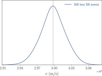
Figure 2. Probability distribution of the speed of light c possible to obtain from the forthcoming LSST survey.
Download figure:
Standard image High-resolution image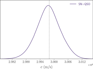
Figure 3. Probability distribution of the speed of light c possible to obtain from the forthcoming LSST survey, with the combination of lensed SNe Ia and lensed quasars.
Download figure:
Standard image High-resolution imageIt is interesting to compare our results with the analysis of Salzano et al. (2015), who first proposed to test the constancy of c using cosmological observables. They noticed that at the redshift zM where the angular diameter distance attains its maximum  . Therefore, whenever one was able to observationally determine zM and reconstruct (with some nonparametric method) DA(z) in its neighborhood, together with the expansion rate H(z), the measurement of
  could be directly obtained. Then, their idea was to use the BAO measurements providing both radial and tangential BAO modes to accomplish this goal. More specifically, Salzano et al. (2015) found that the future missions such as Euclid would be able to give stringent fits on the speed of light at the level of
  , while a VSL of 1% (if any) will be detected at the 1σ level. Further progress in this direction has recently been achieved by Cai et al. (2016), who showed that DES cannot provide better improvement in detecting variation of the speed of light for the 1% case. Another approach was taken in the paper of Cao et al. (2017a), where DA(z) function was reconstructed (using Gaussian processes provided by Seikel et al. 2012) from compact radio sources and H(z) from passively evolving galaxies. The result—first actual measurement of the speed of light using extragalactic objects—confirmed constancy of c at the 6% level (1σ uncertainty level, or 1.4% based on the central fit). Therefore, the combination of strongly lensed and unlensed SNe Ia may achieve considerably higher precision of c measurements than the other popular astrophysical probes including BAO+H(z). We would like to stress that our method of measuring c from lensed SNe Ia not only is competitive with BAOs but also does not rely on any pre-assumed values of cosmological parameters.
There are still many ways in which our technique might be improved. The first is suggested by the methodology applied in our previous study (Cao et al. 2017a). Hence, our method could also be applied to the quasar–galaxy strong-lensing systems with radio quasars acting as background sources. According to the analysis of Oguri & Marshall (2010), LSST should find 3000 lensed quasars, an order-of-magnitude improvement over the lensed SNe Ia. Instead of SNe Ia as standard candles, one may use the angular sizes of the compact structure in intermediate-luminosity radio quasars (Cao et al. 2017a) from the very long baseline interferometry observations and use them as standard rulers at different redshifts (Cao et al. 2017b). Because statistical uncertainty is inversely proportional to  , where N is the number of systems, future observations of lensed quasars will enable us to get more precise measurements of the speed of light. Actually, such a combination of strongly lensed SNe Ia and quasars will result in more stringent constraints on the speed of light at the level of Δc/c = 0.001. The results are shown in Figure 3. Even more important is that in such a case LSST may succeed in detecting the possible existence of VSL effects. Finally, let us emphasize that the improved accuracy of the lens model and the time-delay measurements is crucial to our method. Recently, Liao et al. (2017) proposed a new strategy to simultaneously detect strongly lensed gravitational waves and their electromagnetic counterpart, which will improve the precision of the Fermat potential reconstruction to 0.5%. Given the wealth of available imaging and spectroscopic data, one might be optimistic about achieving much higher precision of lensing time delays in the future. In that case, the precision of c measurements using extragalactic objects would be much higher.
This work was supported by National Key R&D Program of China No. 2017YFA0402600; the National Basic Science Program (Project 973) of China under grant No. 2014CB845800; the National Natural Science Foundation of China under grant Nos. 11503001, 11690023, 11373014, and 11633001; the Beijing Talents Fund of Organization Department of Beijing Municipal Committee of the CPC; the Strategic Priority Research Program of the Chinese Academy of Sciences, grant No. XDB23000000; the Interdiscipline Research Funds of Beijing Normal University; and the Opening Project of Key Laboratory of Computational Astrophysics, National Astronomical Observatories, Chinese Academy of Sciences. J.-Z.Q. was supported by the China Postdoctoral Science Foundation under grant No. 2017M620661. M.B. was supported by the Foreign Talent Introducing Project and Special Fund Support of Foreign Knowledge Introducing Project in China.