Abstract
Direct imaging studies have mainly used low-resolution spectroscopy (R ∼ 20–100) to study the atmospheres of giant exoplanets and brown dwarf companions, but the presence of clouds has often led to degeneracies in the retrieved atmospheric abundances (e.g., carbon-to-oxygen ratio, metallicity). This precludes clear insights into the formation mechanisms of these companions. The Keck Planet Imager and Characterizer (KPIC) uses adaptive optics and single-mode fibers to transport light into NIRSPEC (R ∼ 35,000 in the K band), and aims to address these challenges with high-resolution spectroscopy. Using an atmospheric retrieval framework based on petitRADTRANS, we analyze the KPIC high-resolution spectrum (2.29–2.49 μm) and the archival low-resolution spectrum (1–2.2 μm) of the benchmark brown dwarf HD 4747 B (m = 67.2 ± 1.8 MJup, a = 10.0 ± 0.2 au, Teff ≈ 1400 K). We find that our measured C/O and metallicity for the companion from the KPIC high-resolution spectrum agree with those of its host star within 1σ–2σ. The retrieved parameters from the K-band high-resolution spectrum are also independent of our choice of cloud model. In contrast, the retrieved parameters from the low-resolution spectrum are highly sensitive to our chosen cloud model. Finally, we detect CO, H2O, and CH4 (volume-mixing ratio of log(CH4) = −4.82 ± 0.23) in this L/T transition companion with the KPIC data. The relative molecular abundances allow us to constrain the degree of chemical disequilibrium in the atmosphere of HD 4747 B, and infer a vertical diffusion coefficient that is at the upper limit predicted from mixing length theory.
Original content from this work may be used under the terms of the Creative Commons Attribution 4.0 licence. Any further distribution of this work must maintain attribution to the author(s) and the title of the work, journal citation and DOI.
1. Introduction
The Keck Planet Imager and Characterizer (KPIC) is a new suite of instrument upgrades at Keck II, including a single-mode fiber injection unit (FIU; Delorme et al. 2021; Mawet et al. 2017) that feeds light into the upgraded NIRSPEC (Martin et al. 2018; López et al. 2020), enabling high-resolution spectroscopy (HRS
18
) at R ∼ 35,000 in the K band. By using single-mode fibers to inject light from planets and brown dwarfs at high contrast, KPIC provides suppression of the stellar point-spread function (PSF) at the fiber input and a stable line-spread function (LSF) that is independent of incoming wave-front aberrations (Mawet et al. 2017; Wang et al. 2021b). By observing at high resolution, we can further distinguish between star and planet light from their spectral differences (Mawet et al. 2017; Wang et al. 2017). Recently, Wang et al. (2021b) published the KPIC detections of HR 8799 c, d, e, demonstrating the ability of KPIC to detect molecular lines and measure the rotational line broadening of planets at high contrast (ΔK ≈ 11) and small separations (≈04) from their host star.
The atmospheric composition of a substellar object holds a wealth of information about its formation, accretion, and evolutionary history, as well as fundamental physical processes that shape its atmosphere. It is therefore important to assess how well KPIC and other fiber-fed, high-resolution spectrographs (e.g., Subaru/REACH; Kotani et al. 2020; and Very Large Telescope/HiRISE; Otten et al. 2021) can measure the atmospheric compositions of directly imaged planets and brown dwarfs. Specifically, previous studies of gas giant planet formation have highlighted the carbon-to-oxygen ratio (C/O) and metallicity (e.g., [C/H]) of the atmosphere as informative probes of formation history (e.g., Öberg et al. 2011; Madhusudhan 2012; Piso et al. 2015). To first order, a companion with a C/O and metallicity similar to that of its host star is consistent with formation via gravitational instability in a protostellar disk or fragmentation in a molecular cloud, akin to binary star formation (Bate et al. 2002). On the other hand, differences between the companion and stellar C/O are suggestive of core accretion (Pollack et al. 1996) as the likely formation mechanism, and in that scenario, could be used to constrain where the companion formed in the disk relative to ice lines of major C- and O-bearing molecules (e.g., H2O, CO2, and CO). This picture can be complicated by a variety of effects such as the relative amount of solids incorporated into the planet’s atmosphere (e.g., Madhusudhan et al. 2014; Mordasini et al. 2016; Öberg & Bergin 2016; Gravity Collaboration et al. 2020; Pelletier et al. 2021).
So far, atmospheric characterization of directly imaged companions has mostly relied on low-resolution spectroscopy (LRS) with resolving powers of R ≈ 20–100. LRS is sensitive to continuum emission originating from the deepest observable layer of the atmosphere and modified by opacity sources farther up. Many of these companions have temperatures warm enough for silicate clouds to condense in their atmospheres (Marley & Robinson 2015), and there is much evidence that cloud opacity plays an important role in the spectrum of directly imaged companions and brown dwarfs with L or L/T transition spectral types (e.g., Skemer et al. 2014; Burningham et al. 2017; Gravity Collaboration et al. 2020). However, due to our limited knowledge of cloud physics, a reliable assessment of atmospheric abundances from LRS could be fraught with degeneracies between clouds, the pressure–temperature (P–T) profile, and chemical abundances (e.g., Burningham et al. 2017). In addition, the retrieval results can also be highly sensitive to systematics in different data sets that are combined to obtain a wider wavelength coverage (Wang et al. 2020a). More encouragingly, Mollière et al. (2020) report atmospheric abundances that are relatively robust to clouds and model choices, though Burningham et al. (2021) show that issues such as an unphysically small radius could persist despite improvements in cloud modeling and extensive wavelength coverage (1–15 μm).
Recently, Wang et al. (2022) presented the first atmospheric free retrievals at high resolution for a directly imaged companion. They studied the L-type brown dwarf HR 7672 B (Teff ≈ 1800 K) using KPIC HRS and near-infrared photometry, and measured carbon and oxygen abundances that are consistent within <1.5σ to that of its host star. In this paper, we present a detailed atmospheric study of HD 4747 B using both KPIC HRS (K band) and archival low-resolution spectra (LRS) from 1–2.2 μm that we re-extract in a uniform manner. While the KPIC HRS resolves individual molecular lines and contains direct information about a companion’s atmospheric abundances, LRS provides spectral shape and luminosity measurements, which has the potential to complement the HRS.
Compared to HR 7672 B, HD 4747 B is a colder L/T transition object (Teff ≈ 1400 K) with strong evidence for clouds and a similar color to directly imaged planets such as HR 8799 c, d, e (Crepp et al. 2018; Peretti et al. 2019). Like HR 7672 B, the wealth of prior knowledge available for HD 4747 B makes it a valuable benchmark object to test whether we can make robust inferences with spectroscopic data. First, we are able to precisely measure the dynamical mass of HD 4747 B (Section 2.2). Mass is a fundamental quantity that is poorly constrained for most directly imaged companions (Bowler 2016). Furthermore, given its high mass, HD 4747 B is expected to have formed via direct gravitational collapse in the same cloud or disk as its host star, which means that we can assume chemical homogeneity: the brown dwarf and primary star should share the same chemical composition. Finally, with the companion mass, observed luminosity, and stellar age, we can independently estimate the brown dwarf’s radius from evolutionary models.
In this paper, we use the open-source radiative transfer code petitRADTRANS (Mollière et al. 2019, 2020) to fit the HRS and LRS for HD 4747 B in a “retrieval” framework. The main goals of our study are to measure the atmospheric composition of this brown dwarf companion using both the HRS and LRS, and to present a detailed characterization of its atmosphere, including constraints on clouds, chemical equilibrium or disequilibrium, and the detection of CH4. In this process, we also explore the relative advantages and disadvantages of HRS versus LRS.
This paper is organized as follows: in Section 2, we summarize the system properties including our mass measurement for HD 4747 B. Our spectroscopic data and data reduction procedure is described in Section 3. We then discuss our spectral analysis framework in Section 4. We present individual and joint retrievals of the HRS and LRS in Sections 5, 6, and 7, respectively. We summarize the lessons learned in Section 8, and conclude in Section 9.
2. System Properties
2.1. Host Star
In this section, we summarize relevant properties of the host star. HD 4747 is a main-sequence, solar-type star located ≈19 pc away based on its Gaia eDR3 parallax (Brown et al. 2021). Chromospheric emission in the Ca ii H&K lines is visible in the stellar spectrum (log RHK = −4.72 ± 0.02), which Peretti et al. (2019) used to derive an age of 2.3 ± 1.4 Gyr from the age-log RHK calibration of Mamajek & Hillenbrand (2008). This agrees with the gyro-chronological age estimate of  Gyr from Crepp et al. (2018). These studies also converged on Teff around 5300–5400 K, and a surface gravity log(g) of 4.5–4.65. Of particular relevance to this study are the C/O ratio and metallicity of the host star, since we expect these to be roughly similar to those of the brown dwarf. HD 4747 is found to have a sub-solar metallicity, with [Fe/H] = −0.23 ± 0.05 from Peretti et al. (2019) and [Fe/H] = −0.22 ± 0.04 from Crepp et al. (2018). Previous studies including Brewer et al. (2016) and Peretti et al. (2019) also measured the elemental abundances for the star, but either did not take into account non-local thermodynamic equilibrium (LTE) effects on their oxygen abundances (Amarsi et al. 2019) or do not quote error bars. We instead carry out a new analysis using the method described in Kolecki et al. (2021) to derive the abundances for different elements, and correct the results to account for 3D non-LTE effects (Amarsi et al. 2019) on the results. For this analysis, we used an archival spectrum from FEROS (Kaufer et al. 1997), which covers 350–920 nm at R = 48,000. Using this spectrum, we measure the equivalent widths of absorption lines and compare them to model stellar atmospheres in an iterative approach using the MOOG code (Sneden 1973). From our derived carbon and oxygen abundances, we find C/O = 0.48 ± 0.08. The iron abundance is [Fe/H] = −0.30 ± 0.5, in agreement with previous studies.
Since Fe condenses out for temperatures below ≈1800 K (Marley & Robinson 2015), it is not a relevant gaseous absorber in the photosphere of HD 4747 B. Therefore, the more useful metrics for comparison are C and O. From our analysis above, we find [C/H] = –0.08 ± 0.06 and [O/H] = − 0.02 ± 0.04 for the host star. [C/H] is defined as  -
-  , where NC and NH are the number fraction of C and H, respectively. [O/H] is defined similarly. We adopt Asplund et al. (2009) as our solar reference in order to be consistent with petitRADTRANS, which we use to model the atmosphere of HD 4747 B.
2.2. Orbit and Dynamical Mass
The orbit and mass of HD 4747 B have been measured by several studies using relative astrometry from Keck/NIRC2, host star radial velocities (RVs) from Keck/HIRES, and Gaia-Hipparcos absolute astrometry (Brandt et al. 2019; Xuan & Wyatt 2020). Here, we take advantage of 23 yr of RV observations published in Rosenthal et al. (2021) and the improved precision of the Hipparcos-Gaia Catalog of Accelerations (Brandt 2021) based on Gaia eDR3 (Brown et al. 2021) to update the orbit and mass of HD 4747 B. HD 4747 B shows significant proper motion anomalies (PMa) in both the Gaia and Hipparcos epochs, with signal-to-noise ratios (S/Ns) of 77.2 and 9.1, and the position angle and amplitude of the PMa is consistent with being induced by the brown dwarf companion. For the relative astrometry, we use data points tabulated in Brandt et al. (2019), except for the two GPI epochs measured by Crepp et al. (2018), which we replaced with our new measurements from Section 3.2. We choose not to use the companion RV as measured by KPIC for this fit, because it does not appreciably improve our already well-constrained orbital solution.
To fit the relative astrometry, radial velocity, and absolute astrometry from Gaia and Hipparcos together, we use the orvara package (Brandt et al. 2021b), which is designed to jointly fit these types of data and takes into account the Gaia and Hipparcos astrometry at the epoch astrometry level using htof (Brandt et al. 2021a). We use the priors listed in Table 4 of Brandt et al. (2021b) for the fitted parameters. The posterior is sampled using the parallel-tempering Markov Chain Monte Carlo sampler (Vousden et al. 2016), a fork of emcee (Foreman-Mackey et al. 2013) over 50,000 steps with 10 temperatures and 100 walkers. The fits converged as determined by visual inspection of the chains, and we discarded the first 10% as burn-in. In orvara, the system parallax and other linear parameters are analytically marginalized out to speed up the fits.
The resulting orbit and mass measurements are tabulated in Table 1, while the model fits are shown in Appendix A. We find a companion mass of m = 67.2 ± 1.8MJup, which is consistent with previous values, but more precise. We checked the orvara results with a second fit where we model the Gaia and Hipparcos astrometry using the methodology in Xuan & Wyatt (2020). This gives m = 67.1 ± 2.0MJup, consistent with the orvara result. Furthermore, the companion mass and orbital parameters we find are also consistent with results from orbit fits that only use RV and imaging data (no Gaia-Hipparcos astrometry) from Peretti et al. (2019) and Crepp et al. (2018). We adopt the companion mass from our orvara fit for the spectral analysis in this paper.
Table 1. Selected Parameters from Orbit Fit
| Parameter | Value |
|---|---|
| M (M⊙) | 0.85 ± 0.04 |
| m (MJup) | 67.2 ± 1.8 |
| a (au) | 10.0 ± 0.2 |
| inclination (deg) | 48.0 ± 0.9 |
| ascending node (deg) | 89.4 ± 1.1 |
| period (yr) | 33.2 ± 0.4 |
| argument of periastron (deg) | 267.2 ± 0.5 |
| eccentricity | 0.7317 ± 0.0014 |
| Epoch of periastron (JD) | 2462615 ± 155 |
Note. The dynamical mass of the host star, which is fit as a free parameter, agrees well with isochrone-derived masses from Peretti et al. (2019) and Crepp et al. (2018).
Download table as: ASCIITypeset image
3. Spectroscopic Data
3.1. High-resolution Spectroscopy
3.1.1. KPIC Observations
We observed HD 4747 B on UT 2020 September 28 with Keck/NIRSPEC. The data were collected using the first version of the KPIC FIU (Delorme et al. 2021). The FIU is located downstream of the Keck II adaptive optics system and is used to inject light from a selected object into one of the single-mode fibers connected to NIRSPEC. We obtain spectrum in the K band, which is broken up into nine echelle orders from 1.94–2.49 μm. The observing strategy is identical to that of Wang et al. (2021b). In short, we placed the companion on the fiber with the highest throughput and acquired six exposures of 600 s each, for a total integration time of 1 hr. The relative astrometry of the companion was computed using whereistheplanet.com (Wang et al. 2021a), based on data in Peretti et al. (2019). For calibration purposes, we acquired a pair of 60 s exposures of the host star before observing the companion, and a pair of 60 s exposures of a telluric standard star (HIP 6960) after the companion exposures so as to share nearly the same airmass. Using exposures on the host star, we calculated an end-to-end throughput from the top of the atmosphere to the detector of 1.8%–2.0% during the observations.
3.1.2. Data Reduction
To extract the spectra from the raw data, we follow the procedure outlined in Wang et al. (2021b), which the KPIC team has implemented in a public Python pipeline. 19 The images for all objects were reduced in the same way. First, we removed the thermal background from the images using combined instrument background frames taken during daytime. As shown in Wang et al. (2021b), the thermal background of our data is dominated by the warm optics rather than the sky background. We also remove persistent bad pixels identified using the background frames. Then, we use data from the telluric standard star to fit the trace of each column in the four fibers and nine spectral orders, which give us the position and standard deviation of the PSF (in spatial direction) at each column. The trace positions and widths were additionally smoothed using a cubic spline in order to mitigate random noise. We adopt the trace locations and widths as the LSF positions and widths in the dispersion dimension.
For every frame, we then extracted the 1D spectra in each column of each order. To remove residual background light, we subtracted the median of pixels that are at least 5 pixels away from every pixel in each column. Finally, we used optimal extraction to sum the flux using weights defined by the 1D Gaussian LSF profiles calculated from spectra of the telluric star.
The extracted spectra have a median S/N of ≈8 per pixel element, which has a typical width of 0.2 Å, and consists of a mixture of light from the brown dwarf companion and stellar speckles. The S/N of KPIC is optimized for wavelengths around 2.3 μm, where CO has a series of strong absorption lines. For our analysis, we use three spectral orders from 2.29–2.49 μm, which contain the strongest absorption lines from the companion and have relatively few telluric absorption lines. Note that the three spectral orders have gaps in between them, so we have data over ≈0.13 μm (instead of 0.2 μm; see Figure 3).
As a preliminary analysis, we cross-correlate our KPIC spectra with single-molecule templates assuming Teff = 1400 K and log(g) = 5.5 from the Sonora model grid (Marley et al. 2021). In short, we estimate the maximum likelihood value for both the single-molecule companion flux and speckle flux in the data as a function of RV (radial velocity) shift using the method described in Wang et al. (2021b), which is based on Ruffio (2019). We find that H2O and CO are detected with S/Ns of 8.5 and 13.5, respectively (Figure 1). CH4 is not detected with statistical confidence in this crude analysis, but we present evidence for a weak CH4 detection in Section 5.4.
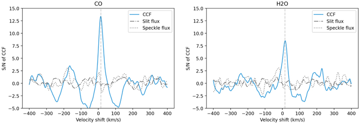
Figure 1. Cross-correlation functions (CCFs) in blue show detections of CO and H2O using three spectral orders of the KPIC HRS. Gray lines represent CCFs of the background flux (from the slit) and speckle flux, whose standard deviations are used as estimates of the CCF noise. The vertical dashed lines at 15 km s−1 show the expected RV of the companion from its known orbit. The strong structure in the blue CCFs outside the peaks arise because we only fit single molecules here.
Download figure:
Standard image High-resolution image3.2. Low-resolution Spectroscopy
3.2.1. Gemini Planet Imager IFS
The Gemini Planet Imager (GPI) observed HD 4747 B on UT 2015 December 24 and 25, in the K1 (1.90–2.19 μm, R = 66) and H (1.50–1.80 μm, R = 46.5) bands, respectively, and the data were published in Crepp et al. (2018). After doing some fits to the published spectrum, we found that the average flux levels of the K1 and H bands are inconsistent, and the error bars appear to be significantly overestimated.
We therefore re-extracted the GPI spectrum using the pyKLIP package (Wang et al. 2015), which models a stellar PSF with Karhunen-Loève Image Processing (KLIP; also known as principal component analysis) following the framework in Soummer et al. (2012) and Pueyo (2016). We tested various model choices to minimize the residuals after stellar PSF subtraction while preserving the companion signal. A key parameter we tuned was the number of Karhunen–Loève (KL) modes. KL modes represent an orthogonal basis for patterns in the images that are used to model the stellar PSF. We chose five and 12 KL modes to subtract the stellar PSF in the H- and K1-band data, respectively. After subtracting the stellar PSF, we first extracted the companion’s relative astrometry in terms of separation and position angle, which are reported in Appendix B (Table 5). Then, we extracted the flux at the companion’s determined location as a function of wavelength, which gave us the raw spectrum. Note that rather than using spectral differential imaging (SDI) to subtract the stellar PSF, we only used angular differential imaging (ADI). For a bright companion like HD 4747 B, ADI is more than sufficient to properly remove the PSF of the star given sufficient parallactic angle rotation.
To flux-calibrate the raw spectrum, we used the satellite spot flux ratios 20 to find the companion-to-star flux ratio. To obtain the observed flux density of the companion, we empirically determined the flux scaling factor R2/d2 by fitting a PHOENIX model (Husser et al. 2013) of the star (Teff = 5400, log(g) =4.5, and [Fe/H] = −0.5) using the star’s Two Micron All Sky Survey J-, H-, and K-band magnitudes (Cutri et al. 2003) and the Gaia G-band magnitudes (Riello et al. 2021). The zero-point fluxes and filter transmission of the photometric bands are downloaded from the Spanish Virtual Observatory (SVO) Filter Service 21 and the Gaia website. 22 To obtain measurement uncertainties, we injected 20 fake companions at the same separation and equally spaced position angles in the data, and repeated the same spectral extraction process. We avoided using the fake injections that were within 20° of the real companion to avoid biasing the fluxes. We inflated the uncertainties on the extracted spectra by 2.5% to account for errors in the stellar flux calibration. The value of 2.5% is estimated by comparing our empirically computed flux scaling factor with the value of R2/d2 of the star (using the radius from Peretti et al. 2019 and the Gaia parallax).
3.2.2. SPHERE IFS
HD 4747 B was observed on UT 2016 December 12 and 2017 September 28 with the Spectro-Polarimetric High-contrast Exoplanet Research (SPHERE; Beuzit et al. 2019). The SPHERE Integral Field Spectrograph (IFS; Claudi et al. 2008) collects data in the YH band from 0.95–1.6 μm (R = 29). The extracted spectrum was published in Peretti et al. (2019), but is not available. We therefore reduced the raw data using the SPHERE pipeline (Vigan 2020), and performed a similar post-processing procedure with pyKLIP as described above for the GPI spectra. The only difference is that we needed to use ADI+SDI to perform PSF subtraction for the SPHERE IFS data, which did not have enough parallactic angle rotation (only ≈02). For the SPHERE IFS data, flux calibration is based on unocculted observations of the host star. We chose to use the 2017 data for our analysis since it was taken under much better observing conditions and yields a slightly higher spectral S/N than the 2016 data, despite shorter integration times.
3.2.3. Results and Comparison with Previous LRS
Our newly extracted GPI and SPHERE spectra are plotted in black circles and squares, respectively, in Figure 2, and available in Appendix B (Table 4). The absolute flux scaling of our GPI spectrum agrees well with the published spectrum in gray from Crepp et al. (2018), but the uncertainties are much smaller. The shape of our new SPHERE spectrum also agrees well with that in Peretti et al. (2019). From the PSF-subtracted images, the brown dwarf companion is detected with a median S/N per wavelength bin of ≈61 and ≈26 in the GPI H and K1 bands, and ≈20 in the SPHERE data. When comparing the extracted spectrum to that of field brown dwarfs from the SPEX library (Burgasser 2014) in Figure 2, we find that the newly extracted GPI spectrum is in better agreement compared to the previously published spectrum. As in Crepp et al. (2018) and Peretti et al. (2019), we find a spectral type near the L/T transition (the best matching spectra were from an L9.5 and T0 dwarf). The SPHERE IFS spectrum increases our wavelength coverage by a factor of ∼2, which we find is important for constraining model atmosphere parameters in our fits to the LRS.
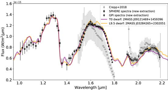
Figure 2. Our extracted LRS of HD 4747 B from GPI and SPHERE are plotted in black circles and squares, respectively, and the published spectra for GPI is shown in gray dots from Crepp et al. (2018). Overplotted in color are spectra of a L9.5 dwarf and T0 dwarf from SPEX (Burgasser 2014), which show good agreement with our extracted spectra, demonstrating that HD 4747 B is consistent with a spectral type near the L/T transition.
Download figure:
Standard image High-resolution image4. Spectral Analysis
4.1. Forward Modeling the KPIC High-resolution Spectrum
Here, we briefly describe the framework to forward model and fit the HRS from KPIC, which follows Wang et al. (2021b). When a companion of interest is aligned with one of the KPIC fibers, the companion light and a fraction of light from the host star’s speckle field are injected into the fiber. At the projected separation of HD 4747 B (≈06), we find the speckles are roughly the same brightness as our companion (Ks
≈ 14.4 from Crepp et al. 2016). Furthermore, the light is transmitted through Earth’s atmosphere and modulated by the instrument optics. Thus, we build two forward models (one for the companion, one for speckles) and jointly fit them as a linear combination. Below we detail how we generate each of the model components.
The companion spectral templates are generated with petitRADTRANS. We shift the templates in wavelength space to fit for the radial velocity. Then, we rotationally broaden the templates by a projected rotation rate  using the fastRotBroad function in PyAstronomy (Czesla et al. 2019), and convolve the templates with the instrumental LSF. The effect of limb darkening is included in petitRADTRANS by integrating intensities along multiple angles between the ray and atmospheric normal.
Next, we multiply the companion model by the telluric response function, which characterizes the atmospheric transmission as a function of wavelength and includes telluric absorption lines. The telluric model is calculated by dividing the spectrum of the standard star (HIP 6960) by a PHOENIX stellar model with matching properties (Teff = 9200 and log(g) = 4.0).
To model the speckle contribution to the data, we use on-axis observations of the host star taken before the companion exposures. These observations are reduced in the same way as the companion spectra, but have a much higher S/N. Unlike the companion models, the host star observations are already modulated by telluric transmission.
The last step is to remove continuum variations. The KPIC spectra are not flux-calibrated and contain a smoothly varying continuum due to stellar speckles and wavelength-dependent atmospheric refraction. Therefore, we apply high-pass filtering with a median filter of 100 pixels (∼0.002 μm) on both the data and models to subtract the continuum following Wang et al. (2021b). To determine the optimal filter size, we carried out a series of injection-recovery tests, and found that ∼100 pixels is best at recovering weak molecular signals for our data set. Larger filter sizes (e.g., 200 pixels or more) do not remove the continuum sufficiently, and smaller filter sizes (50 pixels or less) tend to be overly aggressive at removing weak molecular signals.
Finally, we flux-normalize both the companion and stellar models and multiply them by different flux scaling factors, which are fitted parameters. The flux scales are in units of counts as measured by the NIRSPEC detector. After scaling, the companion and speckle models are added, and the same high-pass filter is applied on the final model before fitting it to the data.
4.2. Atmospheric Retrieval Setup
We implement a “retrieval” framework based on petitRADTRANS to model the data, which means that we freely retrieve the chemical abundances, vertical temperature structure, and cloud properties from the data. Previous studies have used retrievals to model HRS of self-luminous exoplanets and brown dwarfs (e.g., Burningham et al. 2017; Mollière et al. 2020), and show that it can be a powerful alternative to fitting self-consistent grid models, which solve for the abundances and temperature profiles with physical assumptions such as chemical equilibrium. The retrieval approach allows more flexibility to fit the data and can potentially provide much more detailed information about the atmospheric properties, with the caveat that it is important to check for physical plausibility of the models since retrievals need not be self-consistent.
In our main set of retrievals, we fit for the chemical abundances in terms of C/O and atmospheric metallicity [C/H] 23 along with a quench pressure (where the chemical timescale of a certain reaction is equal to the mixing timescale) to allow for disequilibrium chemistry, the temperature profile (Section 4.2.1), the cloud structure (Section 4.2.2), and other parameters such as the radius. We denote these quenched chemistry retrievals to distinguish from free retrievals where the abundances of each gas species is fit independently. Each component of the model is described in the subsections below. We use the correlated-k and line-by-line opacity sampling methods in petitRADTRANS for the low-resolution and high-resolution retrievals, respectively. For high-resolution, we include opacities for CO, H2O, CH4, NH3, and CO2, and for low-resolution, we additionally include Na and K. This is because the alkali lines have wings, which affect the ∼1 μm portion of the LRS, while their opacities are negligible over the portion of the K band covered by our HRS. We repeated our baseline HRS retrieval with Na and K included and found that the addition of these two species did not influence the results or improve the fit.
Because the native high-resolution opacities are at R = 106, much higher than the resolution of our HRS resolution (R ≈ 35,000), we down-sampled the opacity tables by a factor of six in order to speed up the retrievals (by roughly the same factor) and reduce the corresponding computational cost. We checked that the maximum deviation in synthetic spectra obtained by using the down-sampled opacities relative to the full-resolution opacity model is <5% of the minimum HRS error bars. In addition, we repeated our fiducial HRS retrieval with the native opacities (R = 106) and found that it yielded the same results. We re-binned the correlated-k opacities to R = 200 for our fits to the LRS, which has a maximum resolution of 66. We also repeated our fiducial LRS retrieval at the native R = 1000 opacities and found the results are fully consistent.
4.2.1. Temperature Structure and Chemistry
We retrieve the P–T profile of the brown dwarf between P = 10−4–103 bars, which sets the vertical extent of the atmosphere. We use the P–T profile parameterization from Mollière et al. (2020), which has six free parameters. The spatial coordinate is an optical depth τ = δ Pα , where δ and α are the first two parameters. The atmosphere then consists of a high-altitude region (top of atmosphere to τ = 0.1) fitted with three temperature points equidistant in log pressure, a middle radiative region (τ = 0.1 to radiative-convective boundary) that uses the Eddington approximation with T0 as the “internal temperature,” and a lower region (radiative-convective boundary to bottom of atmosphere), which is set to follow the moist adiabatic temperature gradient once the atmosphere becomes unstable to convection (Mollière et al. 2020). We ignore stellar irradiation as a source of heat because the total incident energy on HD 4747 B at periastron (≈2.7 au) is approximately four orders of magnitude less than its luminosity, which is dominated by the brown dwarf’s internal energy.
In our quenched chemistry retrievals, the C/O, [C/H], and P–T profile determine the equilibrium chemical abundances (mass fractions of molecules) as a function of pressure, by interpolating the chemical equilibrium table from Mollière et al. (2020). The opacities we include in the models are listed in Section 4.2. In petitRADTRANS, the abundances of all metals except oxygen are assumed to scale together such that [C/H] = [Si/H] = [N/H], etc. Then, C/O and [C/H] are combined to set the oxygen abundance (Mollière et al. 2020). We use Asplund et al. (2009) as our reference for the solar metallicity in these models.
Finally, we include a quench pressure Pquench, which fixes the abundances of H2O, CO, and CH4 where P < Pquench using the equilibrium values found at Pquench (Zahnle & Marley 2014; Mollière et al. 2020). The inclusion of Pquench allows for the possibility of disequilibrium chemistry, which occurs where the atmospheric mixing timescale is shorter than the chemical reaction timescale. We only include a quench pressure for the net reaction between H2O, CO, and CH4 because these molecules are the only ones detectable in our KPIC HRS (see Section 5.4 for the CH4 detection), and chemical kinetics modeling indicates that the abundances of these three molecules are closely linked to each other by a series of reactions (e.g., Moses et al. 2013). In summary, our quenched chemistry retrievals use C/O, [C/H], and Pquench to set the abundances of each gas species for a given P–T profile.
4.2.2. Clouds
Crepp et al. (2018) and Peretti et al. (2019) analyzed LRS for HD 4747 B and found evidence for a cloudy atmosphere. We summarize their results in Table 2 along with our new measurements. In this study, we consider both clear and cloudy models in order to explore the sensitivity of our retrieved abundances to the assumed cloud properties. For our cloudy model, we use the EddySed model from Ackerman & Marley (2001) as implemented in petitRADTRANS (Mollière et al. 2020). In this model, the cloud particles both absorb and scatter the outgoing photons from the atmosphere according to measured optical properties (Mollière et al. 2019). The cloud particles can be either crystalline or amorphous, and the opacities of the clouds are computed assuming either homogeneous and spherical particles, modeled with Mie theory, or irregularly shaped cloud particles, modeled with the distribution of hollow spheres (DHS; Min et al. 2005; Mollière et al. 2019).
Table 2. Spectral Retrievals Carried Out on HD 4747 B
| Data/Reference | Cloud Model | C/O | [C/H] | Radius (RJup) | log(g) | Teff (K) | B |
|---|---|---|---|---|---|---|---|
| HRS (KPIC) | EddySed (MgSiO3, am) | 0.66 ± 0.04 |

|

|

|

| 1.0 |
| HRS | EddySed (MgSiO3, cd) | 0.67 ± 0.04 |

| 0.90 ± 0.19 |

|

| 1.15 |
| HRS | Clear |

|

|

|

|

| 0.61 |
| HRS | Clear (chemical equilibrium) | 0.60 ± 0.02 |

|

|

|

| 1.6 × 10⁻³ |
| LRS (GPI+SPHERE) | EddySed (MgSiO3, am) |

|

|

|

|

| 1.0 |
| LRS | EddySed (MgSiO3, cd) |

|

| 0.77 ± 0.04 |

| 1443 ± 28 | 0.69 |
| LRS | EddySed (MgSiO3 + Fe, am) |

|

| 0.73 ± 0.03 |

|

| 1.54 |
| LRS | EddySed (MgSiO3 + Fe, cd) |

|

| 0.75 ± 0.03 |

|

| 2.65 |
| LRS | Clear |

|

| 1.10 ± 0.04 | 5.12 ± 0.03 | 1262 ± 16 | 7.0 × 10⁻²⁶ |
| Peretti et al. (2019) | Cloudy retrieval a |

|

| 0.85 ± 0.03 b | 5.40 ± 0.03 | 1350 ± 50 | ⋯ |
| Crepp et al. (2018) | Cloudy grid a ) | ⋯ | ⋯ | ⋯ |

|

| ⋯ |
Notes. The rightmost column lists the Bayes factor (B) for each retrieval, with the EddySed (MgSiO3, am) model as the baseline model with B = 1 (see Section 4.3.1 for an explanation of model comparison with B). We adopt the first row (in bold) as our final results for this paper. A few key parameters and their central 68% credible interval with equal probability above and below the median are listed, along with values for common parameters from two previous studies. For our cloudy models, “am” stands for amorphous cloud particles + Mie scattering, and “cd” stands for crystalline particles + DHS model, as described in Section 4.2.2. Except for the HRS model labeled chemical equilibrium, all of our other models are quenched chemistry retrievals.
a Peretti et al. (2019) carried out cloudy retrievals on their SPHERE spectrum (1.0–1.65 μm) and archival K and L photometry with the HELIOS-R code (Lavie et al. 2017), while Crepp et al. (2018) fitted their extracted GPI spectrum (1.5–2.2 μm) to a cloudy grid model (Saumon & Marley 2008). b Peretti et al. (2019) placed a Gaussian prior of 1.0 ± 0.1RJup on the radius.Download table as: ASCIITypeset image
For HD 4747 B, we consider models with two different cloud species (MgSiO3 and Fe) and properties (amorphous or crystalline particles). We choose to focus on MgSiO3 and Fe for several reasons. First, the condensation curves of these two species intersect the thermal profile of a Teff = 1400 K, log(g) =5.5 object from the Sonora atmospheric model (Marley et al. 2021) at ∼10–50 bars. While the Sonora model is cloudless, it provides a rough estimate of which cloud species are relevant. Second, recent theoretical work has shown that MgSiO3 is expected to be the most important cloud species for substellar objects with Teff > 950 K due to its low nucleation energy barriers and the relatively high elemental abundances of Mg, Si, and O (Gao et al. 2020). Finally, studies using mid-IR spectroscopy from Spitzer have found direct evidence for a MgSiO3 absorption feature at ∼10 μm in field brown dwarfs (Cushing et al. 2006; Luna & Morley 2021), and specifically amorphous MgSiO3 (Burningham et al. 2021). Although MgSiO3 and Fe clouds do not have distinct features in the near-IR, they still impact the near-IR spectrum by contributing a wavelength-dependent opacity. Our baseline model uses amorphous MgSiO3 modeled with Mie theory (abbreviated MgSiO3, “am”) for the clouds. In addition, we also consider models with MgSiO3, “cd,” which assumes crystalline cloud particles modeled with DHS, as well as models with two cloud species (MgSiO3 + Fe) for the LRS.
4.2.3. Methane Opacities
Given that HD 4747 B is located near the L/T transition for brown dwarfs, we might expect to observe methane in its atmosphere. Previous L-band studies have detected methane in field brown dwarfs with spectral types as early as mid-L, or up to Teff ≈ 1800 K (Noll et al. 2000; Johnston et al. 2019). In this study, we adopted the HITEMP CH4 line list from Hargreaves et al. (2020), which we convert into opacities following the petitRADTRANS documentation. When cross-correlating a model generated with the HITEMP CH4 opacities with a late T dwarf, we obtained a CCF S/N of ≈15, in comparison to ≈5 when cross-correlating with a model generated from the default CH4 opacities from ExoMol (Yurchenko & Tennyson 2014) in petitRADTRANS.
4.2.4. Additional Fit Parameters
petitRADTRANS computes the flux density as emitted at the surface of the object. For the LRS, we scale the model by the distance and companion radius, where the radius is another free parameter, and the distance is taken from the Gaia eDR3 parallax (Brown et al. 2021). For the HRS, we also fit the companion’s radial velocity and  , as well as an error multiple term to account for any underestimation in the data uncertainties.
Due to imperfect starlight subtraction in the spectral extraction process, we found that our LRS likely still contains correlated noise from the wavelength-dependence of speckles, as has been noted by several previous studies on high-contrast companions (e.g., Wang et al. 2020b; De Rosa et al. 2016; Samland et al. 2017; Currie et al. 2018; Wang et al. 2021c). This is evident in the residual frames, where we can see speckles at 5%–20% of the companion intensity in the PSF-subtracted images. We therefore adopt a Gaussian process with a squared exponential kernel to empirically estimate the correlated noise in the GPI H, K, and SPHERE YJH bands when fitting models to the data. Following Wang et al. (2020b), we assume that our extracted error bars contain a fraction famp of correlated noise, and 1 − famp of white noise, and fit for famp and the scale of correlation l. This adds 2 × 3 = 6 additional parameters to the retrievals.
As an alternative model, we also tried fitting the LRS with error inflation terms and flux scaling factors for the SPHERE and GPI spectra along the lines of Mollière et al. (2020), but found that our results were very sensitive to our choice of prior for the flux scaling factor. We conclude that our GP model is better suited to account for correlated noise from speckles, and use it in all LRS fits presented in this work.
4.3. Priors
We adopt uniform or log-uniform priors for all model parameters except for the mass, for which we use a Gaussian prior of 67.2 ± 1.8MJup from the dynamical mass measurement (Section 2.2). For the parametric P–T profile parameters, we exclude profiles that contain temperature inversions, as the heat budgets of widely separated companions are dominated by their internal luminosities. For the companion’s radius, we use a uniform prior between 0.6 and 1.2 RJup. When including a quench pressure, we use a log-uniform prior from 10−4 to 103, which is the full pressure range of our models. The priors for all retrieval parameters are tabulated in Table 6 of Appendix C.
4.3.1. Model Fitting with Nested Sampling
We use nested sampling as implemented by dynesty (Speagle 2020) to find the posterior distributions for the model parameters. Specifically, we use 200 live points and adopt the stopping criterion that the estimated contribution of the remaining prior volume to the total evidence is less than 1%. We repeated a few retrievals using 1000 live points and found the evidence remains roughly the same, implying the fits have converged when using 200 live points.
One advantage of adopting nested sampling is that we can use the Bayesian evidence from each fit to calculate the Bayes factor B, which assesses the relative probability of model M2 compared to M1. We will use the Bayes factor to compare different models throughout this paper to determine whether a given M2 is justified over M1. In Table 2, we take a baseline model (MgSiO3, am) to be M1 and compare other models to it. Based on Jeffreys (1983), a model with 100 times lower B than the model with the highest B can be “decisively” rejected. B of ≲10 is considered weak evidence for preferring one model over the other. We first run retrievals with only the HRS (Section 5), only the LRS (Section 6), as well as joint retrievals with both HRS and LRS (Section 7).
5. High-resolution Retrievals (KPIC)
5.1. Overview
From our HRS retrievals of HD 4747 B, we find that both clear and cloudy models yield consistent results for the atmospheric parameters (abundances, temperature structure, and quenching) and bulk properties (radius, radial velocity, and spin). A few selected parameters are plotted in Figure 4 and tabulated in Table 2. The insensitivity of the HRS retrieval results to clouds, a major finding of this paper, is discussed in Section 5.2. In Figure 3, we plot the data, a best-fit model, and residuals for the baseline HRS retrieval. We report values from this retrieval as the final results of this paper, with selected parameters shown in the first row of Table 2 and joint posterior distributions in Appendix C. We also plot the contribution from the planet and star separately at their best-fit flux levels. We compute the auto-correlation function of the residuals and find that there is no evidence for correlated noise or strong systematics. Unless otherwise specified, we quote results from the baseline EddySed cloud model (MgSiO3, am). See Appendix C for the posterior distributions of other parameters from our baseline model.
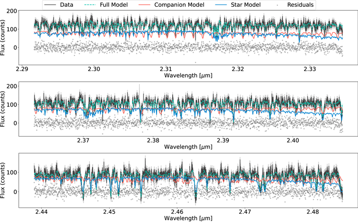
Figure 3. The KPIC HRS used in this study are plotted in black, with error bars inflated to the best-fit value in gray. A sample full model is shown in teal (dashed), and consists of the companion model in orange (which has been RV shifted and broadened), and the stellar model in blue to model the speckle contribution. The companion model shown does not include tellurics to focus on molecular features, but tellurics are included in our fits. The residuals are shown as gray points.
Download figure:
Standard image High-resolution imageTo make sure that we are fitting the correct signal, we check the RV and flux level of the companion. From our orbital posteriors for HD 4747 B, the expected RV shift on the night of our HRS observation is 15.0 ± 0.1 km s−1 in the Earth’s reference frame, which is a combination of the system barycenter velocity, the Earth’s relative velocity with respect to HD 4747, and the companion’s orbital velocity. The fitted RV of 15.0 ± 0.4 km s−1 agrees perfectly with this value (see Figure 4). In addition, the companion flux level in the spectral orders from 2.29 to 2.49 μm is 85 ± 10 counts, comparable to the speckle flux levels in these orders. Taking into account the difference in wavelengths and the difference in integration time (600 s for the companion, 60 s for the on-axis star), we estimate that our measured companion flux corresponds to ΔKs = 8.3 ± 0.3 mag, which is within 3σ of the photometric ΔKs = 9.05 ± 0.14 mag reported by Crepp et al. (2018). The agreement between these contrast values is reasonably good given the time-varying throughput of KPIC (Delorme et al. 2021), and the fact that we subtract out the continuum with high-pass filtering, effects that complicate a direct flux comparison.
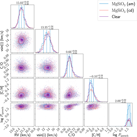
Figure 4. Posterior distributions for five key parameters from HRS retrievals of HD 4747 B, using the EddySed cloud model (MgSiO3, “am” and “cd” in blue and red, respectively), and the clear model in purple. The titles on each histogram show the median and 68% credible interval for the baseline retrieval (MgSiO3, am). Regardless of the cloud model used, the results agree well between different fits for the RV,  , C/O, [C/H] (discussed in Section 5.1), and quench pressure (discussed in Section 5.3).
Download figure:
Standard image High-resolution imageFigure 4 also shows the projected spin rate  km s−1, which is comparable to the rotation rates observed for field brown dwarfs with similar spectral types (e.g., Konopacky et al. 2012). We also plot the retrieved quench pressure Pquench in Figure 4, which indicates that the chemical reaction timescale becomes longer than the vertical mixing timescale at pressures lower than Pquench. Thus, disequilibrium chemistry is clearly affecting the atmosphere (see Section 5.3 for details).
We compute Teff by sampling from our posterior to generate low-resolution models over a large wavelength range (0.5–30 μm) and calculating the integrated flux. We then solve for Teff using the Stefan–Boltzmann law. When computing Teff, we include opacities from Na and K, which are important sources of opacity near visible wavelengths. As shown in Table 2, the retrieved radius and Teff from HRS have broad distributions, which reflect the relatively weak luminosity constraints from the HRS (log(Lbol/L⊙) =  ). This is because the HRS is not flux-calibrated and we remove the continuum in our fits. Comparing to values of radius and Teff from previous work based on LRS (Crepp et al. 2018; Peretti et al. 2019), our retrieved values from the HRS retrievals are consistent at the 1σ–2σ level (see Table 2). We discuss the constraints on these parameters from the LRS in Section 6.2.
We compare our retrieved [C/H], [O/H], and C/O with those of the host star (see Section 2.1) in Figure 5. Our retrieved C abundance agrees well with the host star value, while the O abundance is lower by about 1σ. This results in our retrieved C/O for the companion being higher by about 2σ compared to the stellar value. Here and elsewhere in the paper, we compute the “σ difference” between two measurements by dividing the difference in the two median values by the quadrature sum of the uncertainties from both measurements. We discuss the implications of our measured abundances for HD 4747 B in Section 8.4.
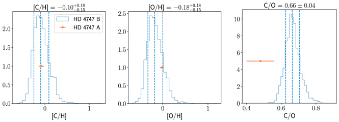
Figure 5. Retrieved C and O abundances (relative to solar) and C/O for HD 4747 B in blue. The titles on each histogram showing the median and 68% credible interval. The red points show the stellar values from Section 2.1. The [C/H] agrees well, [O/H] is consistent within 1σ between the companion and star, and C/O is consistent at the 2σ level.
Download figure:
Standard image High-resolution image5.2. Why Is Our KPIC HRS Insensitive to Clouds in HD 4747 B?
Clouds represent a significant source of uncertainty in many published models of substellar atmospheres (e.g., Burningham et al. 2017; Wang et al. 2020a). However, we find that the retrieved parameters from our KPIC HRS are insensitive to the choice of cloud model for HD 4747 B. As shown in Figure 4, the posteriors for radius, RV,  , C/O, [C/H], and quench pressure are nearly identical across the various models. The same is true for other parameters.
Table 2 shows that the different cloud models are indistinguishable for the KPIC HRS; the clear model fits as well as the cloudy models, with B = 0.61, which does not pass the threshold of B = 10/0.1 to be considered statistically favored/disfavored. This indicates that the data can be fitted adequately without clouds; indeed the cloud parameters for the EddySed models span their respective prior ranges almost uniformly as shown in Appendix C. As we will discuss in Section 6, the LRS shows that the atmosphere of HD 4747 B is cloudy. This implies that cloud opacity must be minimal at the pressures probed by our HRS.
To understand this, we plot in Figure 6 the retrieved P–T profiles (black and blue lines), cloud condensation curves (dashed lines), and emission contribution functions. The left and right panels show results from the HRS and LRS retrievals, respectively. The emission contribution function for HRS shows that we are sensitive to pressures ranging from a few bars, where the continuum forms, up to ≈10−2 bars in the cores of individual lines. Note that the contribution functions use the wavelength axes on the top. In the EddySed model, the cloud base is set at the intersection of the P–T profile and a given cloud condensation curve (dashed lines). For MgSiO3, this corresponds to a pressure of ≈10–20 bars when using our HRS-retrieved P–T profile. As the cloud mass fraction drops exponentially above the cloud base in the EddySed model (controlled by Kzz and fsed), we find that the cloud opacity decreases to negligible levels by the time we reach pressures of a few bars where the continuum forms. For this reason, we do not consider models with Fe clouds in our HRS retrievals, since the Fe cloud base forms even deeper than that of MgSiO3.
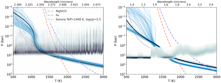
Figure 6. The P–T profiles from our HRS retrieval (left panel) and LRS retrieval (right panel) with the baseline cloud model (MgSiO3, am). In each panel, black lines show the best-fit profile and blue lines are 100 random draws from the posterior. We also show a cloudless Sonora P–T profile (Marley et al. 2021) with similar bulk properties as HD 4747 B in dotted gray. The condensation curves for MgSiO3 and Fe clouds are plotted as dashed lines. We also overplot the emission contribution function as contours, which show the fraction of flux (darker indicates higher fraction) a given pressure layer contributes to the total flux at a given wavelength (Mollière et al. 2019). Thus, these use the wavelength axes, and not the temperature axes. The HRS is sensitive to the continuum forming around a few bars and line cores, which form up to 10−2 bars. Over the same wavelength range of 2.29–2.49 μm, the LRS shows the continuum arises from ≈1–10 bars, consistent with the HRS.
Download figure:
Standard image High-resolution imageTherefore, our KPIC HRS is insensitive to clouds because we cover both a relatively small wavelength range (2.29–2.49 μm) and a range where molecular opacities from H2O, CO, and CH4 are significant. The small wavelength range means that the cloud opacity is effectively constant in wavelength. The strong molecular opacity in HRS allows us to resolve many individual absorption lines and obtain good constraints on the atmospheric composition for molecules present in this region of the spectrum. The opacity of these molecules decreases at shorter wavelength due to decreasing excitation cross sections, so the continuum shifts to higher pressures (deeper down) at shorter wavelengths. This effect is visible in the LRS contribution function, where close to 1 μm, the emission originates from roughly the same pressure as the MgSiO3 cloud base, making the y and J bands particularly sensitive to clouds (see Figure 10).
Could the KPIC HRS be affected by clouds at lower pressures (higher altitudes) than predicted by the EddySed model? Several studies have found that including clouds at lower pressures than predicted by EddySed produces better fits to mid-IR spectra of isolated brown dwarfs (e.g., Burningham et al. 2021; Luna & Morley 2021). As shown in Figure 6, our HRS P–T profiles show a nearly isothermal region between about 0.1–1 bars, which could suggest a degeneracy with clouds (Burningham et al. 2017). To check whether the P–T parameterization affects our results, we run a retrieval with a fixed P–T, namely the self-consistent profile overplotted in gray. We find that all posteriors from this fixed P–T fit overlap within 1σ with those from our baseline retrieval. Thus, we conclude that the isothermal part of the P–T we retrieve is not biasing our conclusions. To further examine the possibility of clouds at lower pressures, we also run an opaque cloud model with infinite opacity below a retrieved pressure, and a gray cloud model that adds a constant cloud opacity at each pressure layer. When fitting the HRS with these more flexible cloud models, we also find consistent results with the baseline model. In the second model, the gray opacity is bounded to lie below ∼0.03 cm2 g–1, and the pressure of the infinitely opaque cloud is required to be deeper than ∼1 bar. Therefore, even with these less constraining cloud parameterizations, we find that our HRS still prefers solutions with minimal cloud opacity.
5.3. Disequilibrium Chemistry with Deep Quenching Pressure
In our retrievals, we include a simple model for disequilibrium chemistry using the quench pressure prescription in petitRADTRANS, which is motivated by Zahnle & Marley (2014). Specifically, the abundances of CH4, CO, and H2O are held constant at atmospheric pressures lower than the retrieved Pquench parameter. We find that when including quenching, the goodness of fit increases drastically compared to fits with full chemical equilibrium. For example, between two clear retrievals with and without quenching, we find that B ≈ 380, in favor of the quenched retrieval. From the Bayes factor interpretation of Benneke & Seager (2013), this represents a detection of quenching at ≈3.9σ significance. The quench pressure retrieved is also highly consistent between retrievals with different cloud models, with 1σ and 2σ intervals of 50−260 and 14−836 bars, respectively (Figure 4). In this section, we explore reasons why the data prefer disequilibrium chemistry in the atmosphere of HD 4747 B. The physical implications of our retrieved quench pressure, including an estimate of the vertical diffusion coefficient (Kzz), are discussed in Section 8.2.
To understand why the data prefer a deep quench pressure, we plot lines of constant log(CO/CH4) volume-mixing ratios (VMRs) along with the best-fit P–T profile from our baseline HRS retrieval in Figure 7. We calculate CO/CH4 from this quenched chemistry retrieval by finding the abundances of each molecule in the chemical grid, iterating over our posterior distribution of C/O, [C/H], and P–T profile. We find that CO/CH4 =  . If the atmosphere was in chemical equilibrium, we repeat our calculation and find that we would expect CO/CH4 =
  , which is 10 times smaller than our retrieved value in the quenched chemistry model. Thus, the relative under-abundance of CH4 relative to CO in our HRS leads our models to prefer a deep quench pressure. The value of CO/CH4 also determines our retrieved the quench pressure, whose 2σ interval is indicated by the thick blue region in Figure 7. Because the P–T profile nearly overlaps the curve of CO/CH4 = 10 at ∼20 bars and deeper, a broad range of quench pressures deeper than ∼20 bars are consistent with the data.
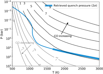
Figure 7. The best-fit P–T profile from our baseline HRS retrieval in blue, with the thicker region indicating the retrieved quench pressure (2σ interval of 14–836 bars). Lines of constant log(CO/CH4) VMRs are shown, with black lines (gray lines) indicating the region where CO (CH4) is more abundant. The P–T profile nearly overlaps with the log(CO/CH4) = +1 line below ∼20 bars, which is where we retrieve the quench pressure to be from the HRS.
Download figure:
Standard image High-resolution imageAs another way to visualize the detection of disequilibrium chemistry, we plot the molecular abundances in VMR as a function of pressure in Figure 8. The solid lines show the VMRs for the HRS quenched chemistry retrieval, while dashed lines show the VMRs for the same model with quenching turned off manually. By comparing the solid and dashed lines, we see that at the pressures probed by our observations, the relative abundances of CO, CH4, and H2O differ by several orders of magnitude between the quenched model and expectations from chemical equilibrium.
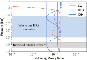
Figure 8. Solid lines: best-fit VMRs of CO, H2O, and CH4 from our baseline HRS retrieval with chemical quenching. Dashed lines: the corresponding VMRs when quenching is turned off (i.e., equilibrium abundances) for the same retrieval. The 1σ quench pressure is indicated by the gray region, and the blue region shows schematically the pressures where our HRS is sensitive. Within the blue region, the relative CO/CH4 ratio can differ by orders of magnitude between the quenched abundances and the equilibrium abundances.
Download figure:
Standard image High-resolution image5.4. Detection of Methane in the HRS
In this section, we take a closer look at the relatively weak methane absorption signal in our HRS, which leads us to prefer quenched models where the CO/CH4 ratio is a factor of 10 higher than predicted in models assuming chemical equilibrium. We confirm the presence of detectable levels of methane in the HRS by running a pair of free retrievals, one with only H2O and CO, and one with H2O, CO, and CH4. The results of these retrievals are listed in Table 3. In these free retrievals, we fit the abundances of each absorbing species independently and assume a constant abundance as a function of pressure. Although we also considered models that included NH3 and CO2, we only obtained upper limits on their abundances, and therefore excluded them from our fits in this section. Finally, given the insensitivity of the HRS to clouds, we carry out these tests with the clear model to save computation time.
Table 3. Free Retrievals Carried Out on HD 4747 B for Validating the CH4 Detection in the KPIC HRS (Section 5.4)
| Molecules | log(CO) | log(H2O) | log(CH4) | B |
|---|---|---|---|---|
| CO, H2O |

|

| ⋯ | 1 |
| CO, H2O, CH4 |

|

| −4.82 ± 0.23 | 84 |
Note. We list the log volume-mixing ratios of molecules included, and the Bayes factor between the model with and without CH4.
Download table as: ASCIITypeset image
We find that the data strongly prefer the model with CH4, with a Bayes factor of 84 (3.4σ significance; Benneke & Seager 2013). As shown in Table 3, we obtain log(CH4) = −4.82 ± 0.23 from the free retrieval, and the CH4 posterior in Figure 9 shows no strong covariance with the abundances of either CO or H2O. If the atmosphere was in chemical equilibrium, we would expect a CH4 VMR that is 10 times higher than what we retrieve, according to the same calculation described in Section 5.3. We note that the abundances from the free retrieval with CH4 also agree well with the corresponding VMRs from our quenched chemistry retrievals. This is not surprising given the deep quench pressure we retrieve, which makes the molecular abundances constant in the regions where our HRS is sensitive (see Figure 8).
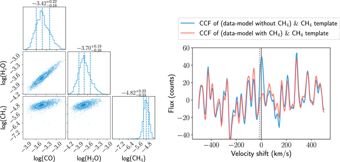
Figure 9. Left panel: joint posterior distributions of the log(VMR) of CO, H2O, and CH4 from a KPIC HRS retrieval where we directly fit the molecular abundances and assume they are constant across pressure. Right panel: CCFs of a pure CH4 template with (KPIC data—model without CH4) in blue, and the CCF of the CH4 template with (data—model with CH4) in red. The CH4 template is generated with best-fit parameters of the full model with CH4, CO, and H2O and manually setting opacities of CO and H2O to zero. The gray solid line indicates the companion rest frame, and the gray dotted line is the telluric rest frame. The residuals are taken from two spectral orders (2.29–2.41 μm) with stronger CH4 detection.
Download figure:
Standard image High-resolution imageWe separately visualize the CH4 detection in cross-correlation space by carrying out an analysis similar to that described in Zhang et al. (2021). First, we make a “pure CH4 template” from the best-fit companion model with CH4, H2O, and CO by manually setting the abundances of H2O and CO to zero. If the model without CH4 is fitting poorly due to its inability to fit CH4 lines in the data, we would expect the residuals of this model, which we denote R = (data—model without CH4), to contain CH4 lines. Therefore, we cross-correlate R with the pure CH4 template, plotted as the blue CCF in Figure 9. In addition, we plot the CCF of  (data—model with CH4) with the pure CH4 template in red for comparison. The blue CCF shows a peak at 0 km s−1 (solid gray line), where we expect a real signal to be since the models have been shifted by the best-fit companion RV. If the residuals were dominated by telluric CH4 for example, the CCF peak would appear at the dotted gray line (negative of the RV, or −15 km s−1). Thus, even though the height of the CH4 peak in the blue CCF is small compared to the surrounding structure, the fact that it is located at the companion RV is evidence of a real signal from CH4.
In our CCF framework, the y-axis is the estimated flux level (in counts) of the companion signal from a least-squares minimization. As shown in Figure 9, we find a flux level of ≈50 counts for CH4, which is an estimate of the companion flux in the residuals. Importantly, this value is consistent with the flux value found when we repeat the same CCF analysis with H2O (i.e., comparing a model with only CO and CH4 and the baseline model of CO, H2O, and CH4). For a molecule such as NH3, which we see no evidence of in the KPIC HRS, the flux value from the CCF becomes unbounded as the least-squares routine used for computing the CCF fails to converge.
Finally, we check for crosstalk between H2O and CH4 by cross-correlating R with the pure water template and detect no CCF peaks. Furthermore, we note that in a retrieval with only CO and CH4 (no H2O), the retrieved CH4 abundance is consistent with the value from the full model including CO, H2O, and CH4.
We therefore conclude that the data strongly favor the presence of detectable levels of methane in the HRS, with an abundance significantly lower than that predicted by equilibrium chemistry models. The detection of methane at log(CH4) = −4.82 ± 0.23 demonstrates the ability of KPIC to retrieve species that are more than an order of magnitude lower in VMR than the dominant molecular constituents in the data, in only 1 hr of integration time.
6. Low-resolution Retrievals (GPI + SPHERE)
6.1. Overview
In this section, we present the results from our fits to the LRS and compare our retrieved parameters to those from the HRS fits. We fit the LRS using the same models as before. These include one clear model and four different implementations of the EddySed cloud model where we vary our assumptions about the unknown cloud properties. The cloudy models consist of two MgSiO3 retrievals with am and cd particles (explained in Section 4.2.2), and two retrievals with MgSiO3 and Fe clouds (again, am and cd). In Figure 10, we plot the data, best-fit cloudy and clear models, the residuals, and the GP models of the residuals. The posteriors for a few key parameters from these retrievals are plotted in Figure 11 and tabulated in Table 2. See Appendix C for the posterior distributions of other parameters in the baseline model.
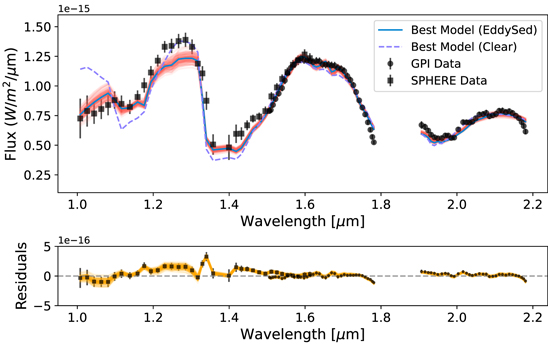
Figure 10. Top panel: best-fit cloudy model (EddySed + MgSiO3, am) in blue and random models drawn from the posterior in light orange for an LRS retrieval of HD 4747 B. The best-fit clear model is overplotted in dashed purple, which fits visibly worse from ≈1.0 to 1.2 μm. Bottom panel: the residuals of the cloudy model shown in error bars, along with random draws of the GP models for the residuals in orange.
Download figure:
Standard image High-resolution image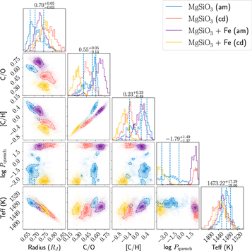
Figure 11. Posterior distributions for a few key parameters from LRS retrievals of HD 4747 B, using the EddySed model with MgSiO3 clouds (blue: amorphous; red: crystalline), and MgSiO3 + Fe clouds (purple: amorphous, yellow: crystalline). The titles on each histogram show the median and 68% credible interval for the MgSiO3, am model. The results disagree by as much as 3σ, especially in 2D space, and display strong covariance between C/O and [C/H]. The radius retrieved is also generally smaller than predicted by evolutionary models.
Download figure:
Standard image High-resolution imageWhen comparing the clear and cloudy models in Figure 10, we see that the data shortward of ∼1.2 μm is poorly fit by models without clouds. This causes the clear model to have B ≈ 7 × 10⁻²⁶; it is overwhelmingly ruled out compared to the baseline EddySed model. In addition, when we plot the models over a larger wavelength range in Figure 12, we find that the cloudy models agree with the NIRC2 L-band photometry from Crepp et al. (2016), while the clear model overpredicts the L-band flux by ≈2σ. We did not include these photometric points in our retrievals.
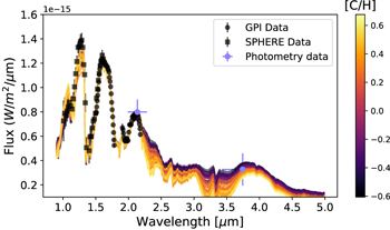
Figure 12. Random models drawn from the posterior of the baseline LRS retrieval (MgSiO3, am), plotted over a larger wavelength range and color-coded by [C/H], the metallicity. There is a gradient in [C/H] in the L (≈3.4–4.2 μm) and M (≈4.55–4.8 μm) bands, which can be distinguished with a comparable S/N LRS in these bands. The GPI and SPHERE data are shown in black, and we also overplot the photometric data points from Crepp et al. (2016), which are not included in the retrievals but nonetheless agree with our models.
Download figure:
Standard image High-resolution imageFigure 10 shows that the SPHERE J-band data from ≈1.2–1.35 μm is not well fit by even the cloudy model, which could either be caused by model mismatch or speckle contamination that artificially raises the flux. The GP model finds that ∼60% of the SPHERE error bars and ∼90% of the GPI error bars are from correlated noise, with correlation length scales of ∼6 and ∼2 wavelength channels, respectively. This confirms our initial intuition that the noise in the SPHERE and GPI images is likely dominated by correlated speckle noise based on visual inspection of the images. For the SPHERE data set, we estimate that the retrieved length scale is roughly equal to the number of steps that a speckle would move across the PSF for our brown dwarf’s separation; indeed, we see speckles moving across the companion PSF in the reduced images. Overall, the SPHERE spectrum is less reliable than that from GPI because only four exposures are available, compared to the ∼40 exposures from GPI.
Finally, the P–T profile retrieved from our baseline LRS retrieval shows a bimodal distribution (see Figure 6). The degeneracy seen here may be related to issues with the LRS (see Section 6.3).
6.2. Comparison with Prior Knowledge
Because the LRS is flux-calibrated, we can check whether our retrieved radii and effective temperatures are physical and consistent with prior knowledge for this benchmark companion. Using the known age and mass of HD 4747 B (3 ± 2 Gyr and m = 67.2 ± 1.8 MJup), we interpolate the COND evolutionary models (Baraffe et al. 2003) to find a model-predicted radius of  , and a predicted
  K. Peretti et al. (2019) compared the SPHERE spectrum of HD 4747B to those of field brown dwarfs to derive a more tightly constrained Teff = 1350 ± 50 K (see Table 2), which we adopt in the subsequent discussion.
We calculate the effective temperatures of the models in our retrievals by integrating the flux over 0.5–30 μm. For the baseline EddySed model, we find  K, and a radius of
  . Compared to prior expectations, however, the radius retrieved is too small by ≈1.5σ while Teff is too high by ≈2σ. From substellar evolutionary models, the minimum possible radius of a brown dwarf should be ≈0.74 RJup, which is imposed by electron degeneracy pressure (Chabrier et al. 2009). We find that Teff and radius are correlated in the LRS retrievals, as shown in Figure 11, which is expected as different combinations of these two parameters can produce the same total luminosity. However, our total luminosity agrees well with the luminosity predicted by evolutionary models.
Several previous retrieval studies have also found smaller-than-expected radii for L dwarfs, which may be attributed to the presence of heterogeneous surface features, such as patchy clouds, that are not captured in current 1D retrieval frameworks (e.g., Gonzales et al. 2020; Kitzmann et al. 2020; Burningham et al. 2021). On the other hand, Gonzales et al. (2021) retrieved a radius consistent with evolutionary models for a seemingly cloudless L dwarf. Whether the radii from evolutionary models are correct is an assumption that is now being tested by a growing sample of transiting brown dwarfs from TESS (e.g., Carmichael et al. 2020).
In our retrievals with both MgSiO3 and Fe clouds, we retrieve slightly larger radii that are more consistent with the evolutionary model prediction. This could indicate that a single cloud model (MgSiO3) may be inadequate in attenuating the flux from the deep atmosphere. However, models with two cloud species do not improve the fit significantly (B = 1.5–3 compared to the baseline model with MgSiO3 only). Furthermore, the MgSiO3, cd model actually has the largest retrieved radius, but our data cannot distinguish between crystalline and amorphous particles. We conclude that our retrieved radius is sensitive to aspects of the cloud models that are poorly constrained by the existing data for this object.
6.3. LRS at Longer Wavelengths Could Improve Abundance and Cloud Constraints
While the LRS can provide tighter constraints on the cloud parameters and radius compared to the HRS, we find that many retrieved parameters, including the atmospheric abundances, are very sensitive to model choices. In Figure 11, we overplot the posterior distributions of a few parameters from our four EddySed models. The retrieved C/O and [C/H] have large uncertainties and can disagree at the 3σ level between models. The values also span a significant portion of the parameter space (>1 dex in metallicity), and show much stronger covariance compared to those measured from the HRS (see Figure 4). However, all cloudy models fit the LRS well, with Bayes factors within a factor of ∼3 (see Table 2), so we cannot distinguish between them.
We note that Mollière et al. (2020) were able to obtain much better constraints on the composition of HR 8799e, which also has a cloudy atmosphere, using LRS data sets from 0.95–2.5 μm. Their LRS had an S/N between 4 and 11 per wavelength bin, much lower than the S/N of our LRS (between 20 and 60 per wavelength bin). Unlike Mollière et al. (2020), however, our study does not have LRS in the second half of K band (2.2–2.5 μm), which contains a strong CO bandhead as well as significant H2O and CH4 opacities. When we compute the CO abundances from our LRS retrievals, we find that they are not well constrained, with 1σ intervals that are ≳3 wider than the CO constraint from HRS. In Figure 12, we plot random draws of our baseline model color-coded by metallicity out to 5 μm. As shown, the models diverge quickly in the 2.2–2.5 μm range. The fact that we miss this crucial wavelength region could explain why Mollière et al. (2020) obtained more robust constraints on atmospheric abundances and P–T profiles that agree better with self-consistent models than we do, despite using data with a lower S/N.
Figure 12 also shows a clear gradient in metallicity beyond 2.5 μm. In some of our cloudy LRS retrievals, we see a covariance between metallicity and cloud mass fraction, where lower metallicities correspond to higher cloud mass fractions as well as larger, more physically consistent radii (see Figure 11). The degeneracy between metallicity and cloud mass fraction might arise because both molecular opacities and clouds contribute opacity, and our data has insufficient wavelength coverage to probe more regions where the gas and cloud opacities are sufficiently different. From the LRS retrievals, we consistently find a factor of ∼2–3 more CH4 and H2O than observed in the HRS, implying that the LRS retrievals could be compensating for our imperfect cloud models by increasing the gas opacities.
Using a more flexible cloud model might alleviate some of these issues. For example, Burningham et al. (2021) retrieved the 1–15 μm LRS of a field L dwarf and found the data preferred silicate clouds much higher up than the predicted cloud base locations from condensation curves. In addition, their retrieved cloud particles also have smaller sizes (submicron) than predicted by the EddySed model (a few microns). Similarly, Luna & Morley (2021) found that submicron cloud particles at lower pressures than predicted by EddySed are required to fit the mid-IR silicate feature (≈8–10 μm) of many L dwarfs. They found that the microphysical cloud model CARMA (Turco et al. 1979; Toon et al. 1988; Gao et al. 2018) allows them to fit their data much better and even place constraints on which cloud species are producing the observed absorption feature.
Both of the above-mentioned studies benefitted from data at ∼10 μm that significantly helped with constraining cloud properties. Thus, to obtain better abundance measurements with LRS, it is not only important to obtain full coverage in the near-IR (which we lack), but also to acquire data in the mid-IR. JWST can obtain low- and medium-resolution spectroscopy of brown dwarfs spanning the near- to mid-IR wavelengths using the NIRSpec and MIRI instruments. Future ground-based instruments such as SCALES at Keck (Stelter et al. 2020) will also provide LRS in the mid-IR.
7. Joint Retrievals
In this section, we describe the results of joint retrievals to both the HRS and LRS for HD 4747 B. In practice, we set up two radiative transfer routines with petitRADTRANS using line-by-line (for HRS) and correlated-k (for LRS) opacity sampling, respectively. The HRS and LRS models share the same atmospheric parameters and priors, but each has some unique parameters (e.g., RV and  for HRS, GP kernel parameters for LRS). Within one nested sampling retrieval, we add the log likelihoods from the HRS and LRS components at each step of sampling to get the total log likelihood. We consider both clear and cloudy EddySed models for our joint retrievals.
Because the LRS prefer clouds, the cloudy model (MgSiO3, am) is overwhelmingly preferred in our joint retrieval, with a Bayes factor in excess of 1034 compared to the clear model. From the cloudy model, we retrieve C/O = 0.70 ± 0.03 and [C/H] = 0.34 ± 0.07. The retrieved uncertainties on these parameters are lower than in the HRS-only retrieval (which had C/O = 0.66 ± 0.04 and [C/H] =  ). In addition, the C/O from our joint fit is consistent with the C/O from our HRS fit. This is not surprising, because the HRS places tight constraints on the relative line depths (and hence the relative abundance ratios) of CH4, H2O, and CO. However, the joint fit pushes the metallicity to higher values, which corresponds to increased gas abundances as shown in Figure 13. The joint fit results translate to a >4σ discrepancy in [C/H] between HD 4747 A&B, while there is no discrepancy if we take the results from the HRS fit. This implies that the joint fit might be compensating for inadequacies in modeling clouds by increasing the gas opacities, as discussed in Section 6.3 for the LRS-only case. We ran additional joint retrievals where we varied the cloud parameters (e.g., adding Fe clouds) and found similar results.
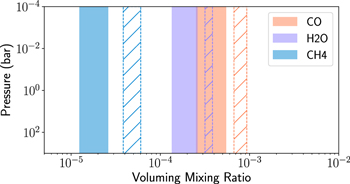
Figure 13. Filled areas: 1σ intervals for the CO, H2O, and CH4 abundances from our KPIC HRS retrieval. Hatched areas: the same for a joint retrieval (HRS + LRS). The retrieved abundances are two to three times higher in the joint retrieval, while the relative abundance ratios between species stays roughly the same (which produces a similar C/O). This highlights the fact that HRS is better at constraining relative abundances than absolute abundances.
Download figure:
Standard image High-resolution imageIf we compare the log likelihoods of the HRS part of the joint fit to that from the HRS-only fit, we find that the HRS is fit less well by ≈e10 (which translates to ≈4σ) in the joint fit, implying a trade-off between fitting the LRS and HRS. We can qualitatively compare the LRS S/N per wavelength bin to the CCF S/N of the HRS, which approximates the total constraining power of the HRS. When including all molecules in our model, we find a CCF S/N of ≈15 for the HRS. For the LRS, the average S/N per wavelength bin is ≈20 for the SPHERE YJH data and ≈60/30 between the GPI H/K1 data. This explains why the joint fits prioritize fitting the LRS at the expense of the HRS.
As discussed in Section 6, the LRS are very model-sensitive and additionally contaminated by correlated noise. For this reason, we adopt the HRS-only results as the best estimate of HD 4747 B’s atmospheric properties in this paper (see first row of Table 2). We leave it to future work, preferably aided by longer wavelength coverage in LRS, to achieve a more satisfactory joint retrieval.
8. Discussion
8.1. Next Steps for High-resolution Spectroscopy
Our KPIC HRS provides a better handle on the atmospheric abundances of HD 4747 B, and is less sensitive to model choices than our LRS. In fact, our K-band HRS is essentially agnostic to clouds in the brown dwarf’s atmosphere; all retrieved parameters are consistent independent of our chosen cloud model (Figure 4). As discussed in Section 5.2, this is because our HRS covers a wavelength region (2.29–2.49 μm) of high molecular opacity, and probes emission across a wide range of atmospheric pressures where cloud opacity is negligible (up to 10−2 bars in line cores). While clouds affect the continuum near 1 μm in the LRS, they have little effect on the line depths across the wavelength range of our HRS. The relative line depths are sensitive to relative molecular abundances, which directly constrain C/O. These results advocate for using HRS to measure atmospheric abundances.
In the future, it is important to explore whether these findings hold true for other substellar objects. In upcoming papers, we will present KPIC HRS retrievals of brown dwarf companions and giant planets spanning a range of effective temperatures and surface gravities. Ultimately, it would also be useful to constrain cloud properties with HRS. For transmission spectroscopy, Gandhi et al. (2020) found that their simulated near-IR HRS for warm Neptunes is more sensitive to molecular abundances than LRS for the same reasons highlighted in this study. While both clouds and metallicity affect the line depths in HRS, Gandhi et al. (2020) showed that increasing the wavelength coverage (e.g., going from 0.9–1.7 μm to 0.9–2.5 μm) helps distinguish between clouds and metallicity and provides better constraints on both. Thus, if we wish to obtain constraints on clouds and abundances at the same time, it would be important to extend our current HRS to a broader range of wavelengths. KPIC Phase II will allow us to obtain L-band data (≈3.4–4.1 μm) to complement existing K-band data (Delorme et al. 2021), and future upgrades could benefit from including the H and J bands as well.
In this study, we have assumed that the atmosphere of HD 4747 B is globally uniform. However, it would be important to examine the impact of 3D effects, including nonuniform cloud coverage. Past studies with photometry or LRS show that many brown dwarfs exhibit clear rotational variability signals (e.g., Apai et al. 2013; Biller et al. 2018; Zhou et al. 2018; Manjavacas et al. 2021; Vos et al. 2022), which appear to be caused by inhomogeneities in their cloud properties. Therefore, time-resolved observations are important to understanding clouds and 3D effects.
With HRS, we can use the time-varying line depth and shape to map the 2D brightness distributions of these objects (e.g., Crossfield et al. 2014). In this paper, we used 1 hr of KPIC data for HD 4747 B. Given our measured  and assuming a radius of 0.8RJup, we would expect a 5 or 7 hr rotation period if i is equal to the orbital inclination or i = 90°. Thus, it may be possible to sample a full rotation period within a single observing night, with the caveat that measurements of the true rotation period remain difficult for high-contrast companions (Biller et al. 2021).
8.2. Methane and the Presence of Disequilibrium Chemistry
Our HRS retrievals indicate that the ratio of CO/CH4 (VMR) is ≈10 times higher than expected by equilibrium chemistry (see Section 5.3). To gain more physical intuition, we convert the quench pressure from our HRS retrievals to an estimate of the vertical diffusion coefficient, Kzz. To do this, we match the chemical timescale of the CO-CH4 reaction from Zahnle & Marley (2014) with the mixing timescale τmix = L2/Kzz. While the length scale L is typically taken to be the pressure scale height H, for lack of a better estimate, Smith (1998) showed that this assumption is not valid across several reactions in the atmospheres of Jupiter and Neptune. In fact, Smith (1998) found that L ≈ 0.1H, which changes the inferred Kzz by two orders of magnitude. Similarly, Ackerman & Marley (2001) also noted that the mixing length is generally shorter than the pressure scale height H in stable atmospheric regions. Due to the uncertainty in L, we adopt L = α
H, where α is a scaling factor, and  (μ: mean molecular weight, g: surface gravity, T: the local temperature). For each value of quench pressure from our posteriors, we compute the necessary quantities to derive a posterior for Kzz. For instance, if α = 0.1, we find Kzz = 5 × 10⁸ − 1 × 1012 cm2 s−1 (1σ). On the other hand, if α = 1, we obtain Kzz = 5 × 10¹⁰ − 1 × 1014 cm2 s−1.
There have been few quantitative measurements of Kzz for substellar companions. Miles et al. (2020) used M-band LRS to constrain the CO abundance and estimate Kzz for seven field brown dwarfs. However, their objects have Teff between 250 and 750 K, much colder than HD 4747 B. In terms of objects with Teff ≳ 1000 K, Barman et al. (2015) reported a detection of CH4 in HR 8799b (Teff ∼ 1000 K) with Keck/OSIRIS data, which they used to estimate Kzz between 106 and 108 cm2 s−1. However, this CH4 detection was not confirmed by an independent study (Petit dit de la Roche et al. 2018), and recently Ruffio et al. (2021) concluded that future higher-resolution follow-up is needed to resolve the discrepant CH4 signal strengths found by different analyses. Ruffio et al. (2021) pointed out that if the CH4 abundance was overestimated by Barman et al. (2015), that would imply a larger Kzz. Using LRS, Mollière et al. (2020) found a well-constrained quench pressure for HR 8799e (Teff ∼ 1100 K) from petitRADTRANS retrievals, which could similarly be converted to a Kzz constraint. In summary, our finding HD 4747 B, which is ∼300–400 K hotter than HR 8799 b and e and much older (a few Gyr; Section 2.1) than most directly imaged planets, represents an important new data point because hotter objects are expected to be closer to equilibrium, making chemical disequilibrium processes harder to detect (e.g., Moses et al. 2013).
Zahnle & Marley (2014) provided an upper limit for Kzz from mixing length theory (Gierasch & Conrath 1985) assuming full convection. For HD 4747 B, their Equation (4) translates to an upper limit of ≈109 cm2 s−1. Depending on α, our retrieved Kzz either exceeds this upper limit by ≳2σ (if L = H), or is very close to this limit (if L = 0.1H). Together, this suggests that convection is driving the vertical mixing in HD 4747 B, and that the mixing efficiency is likely close to its predicted maximum. We check whether our inferred Kzz makes sense by comparing them to those predicted by self-consistent atmospheric models with disequilibrium chemistry from Karalidi et al. (2021) and Mukherjee et al. (2022). For an object with properties similar to HD 4747 B, our measured CH4 VMR is consistent with Kzz ∼ 108–1012 in these models (with the assumption that L = H). These values of Kzz are roughly consistent with our estimate based on Pquench, and also near the upper limit from Zahnle & Marley (2014). On the modeling front, it would be valuable to carry out 3D hydrodynamical simulations (e.g., Zhang & Showman 2018; Tan & Showman 2021) of brown dwarf interiors to independently estimate Kzz (Tan 2022) and compare the results to that inferred by our data. Such simulations could also reveal which physical processes might cause a discrepancy between mixing length theory and our observations.
8.3. Dynamical versus Spectroscopic Mass Constraints
For a majority of substellar companions observed by direct imaging, there are no dynamical mass constraints. To assess whether our mass prior plays an important role in the results, we repeat our HRS and LRS retrievals with the baseline cloud model but use uniform priors in mass from 10 to 100 MJup (“free-mass”). For the HRS free-mass retrieval, we find that all parameters change by less than 1σ compared to the mass-prior retrieval. The mass itself shows a broad distribution (33–76 MJup at 1σ) that encompasses the dynamical mass. Because our KPIC HRS is not flux-calibrated, the radius is not well constrained. In this case, we get large uncertainties in the spectroscopic mass because mass is inferred from the retrieved surface gravity, which depends on the poorly constrained radius.
Our LRS free-mass retrieval also yields posteriors for all parameters that are consistent between 1σ and 2σ with the mass-prior retrieval. Furthermore, the mass retrieved by the LRS is  , which agrees within about 1σ with the dynamical mass. This provides confidence that reasonable mass constraints can be placed on substellar objects from LRS. The radius retrieved is 0.77 ± 0.03RJup, consistent with evolutionary model predictions and close to the radius from the mass-prior retrieval, suggesting the two retrievals find a similar surface gravity.
8.4. Atmospheric Abundances of HD 4747 AB
We retrieve [C/H] and [O/H] values that are 1σ consistent with those of the host star, as discussed in Section 5.1. Both the companion and the star are mildly sub-solar in terms of their metal content. However, our retrieved C/O = 0.66 ± 0.04 is higher by approximately 2σ than the stellar C/O =0.48 ± 0.08.
The question is whether the marginal discrepancy in C/O is from astrophysical or systematic reasons. For example, Wang et al. (2022) carried out retrieval experiments on simulated HRS (2.2–2.35 μm, R = 35,000) and found that their formal error bars are likely underestimated due to systematic errors at the ∼0.15 level in C/O. Using KPIC HRS from 2.23–2.33 μm, they found ≈1σ–1.5σ discrepancies between the [C/H] and [O/H] abundances of HR 7672 A and B, another benchmark brown dwarf system. On an earlier study of benchmark brown dwarfs, Line et al. (2015) quoted 1σ uncertainties of 0.2–0.3 in their brown dwarf C/O (much larger than our formal C/O uncertainty of 0.04), and concluded that a 2σ agreement between the stellar and companion C/O is sufficiently good given the caveats. It is also possible that the uncertainties on stellar abundances are underestimated given non-LTE effects (Line et al. 2015).
Another factor that might contribute to the 2σ discrepancy in C/O is uncertainties in the chemistry of condensates. The chemical model of petitRADTRANS we use accounts for the equilibrium condensation of various species and reports the global (rather than gas phase) C and O abundances (Mollière et al. 2019). In particular, species such as MgSiO3 and Mg2SiO4 contain three or four oxygen atoms per molecule, and are expected to hold a significant portion of O (Line et al. 2015). From our HRS retrievals, we find that ≈18% of O is condensed into solids such as MgSiO3. In order to decrease the global C/O of the brown dwarf by ≈0.1 (therefore making the companion and stellar C/O agree at the 1σ level), we require a ∼20% increase in the net O abundance. Keeping everything else unchanged, this means the MgSiO3 mass fraction, which is predicted by the chemical model to be ∼2 × 10⁻³ in our retrievals, needs to be doubled to ∼4 × 10⁻³. From the LRS retrievals, the cloud base MgSiO3 fraction can be as high as 10−2. Therefore, a factor of ∼2 uncertainty in the abundance of MgSiO3 could make our C/O consistent at the 1σ level with the stellar value.
Given these caveats, we conclude that the 2σ difference between our retrieved C/O for HD 4747 B and the stellar value is not significant, and HD 4747 AB are consistent with being chemically homogeneous. Chemical homogeneity is expected by models where brown dwarf companions form via gravitational fragmentation in molecular clouds (e.g., Padoan & Nordlund 2004) or massive protostellar disks (e.g., Stamatellos et al. 2007). Simulations suggest that brown dwarfs typically form as part of unstable, high-order multiple systems, which undergo chaotic interactions that reduce the multiplicity over time (e.g., Bate et al. 2002; Thies et al. 2010; Bate 2012). With a semimajor axis of 10 au, HD 4747 B is unlikely to have been directly affected by such encounters, but its relatively high orbital eccentricity (≈0.73) could encode such a dynamically “hot” past.
9. Conclusions
Using high-resolution spectrum (R ∼ 35,000) obtained by Keck/KPIC, we retrieve [C/H] =  , [O/H] =
 , and C/O = 0.66 ± 0.04 for the benchmark brown dwarf companion HD 4747 B (formal error bars). The C and O abundances are consistent with the stellar values to ≲ 1σ, while the C/O ratio is consistent at the 2σ level, as expected for a formation scenario akin to that of binary stars. This shows that we can measure the atmospheric abundances for high-contrast substellar companions to the 20% level with KPIC and our current modeling framework, which Wang et al. (2022) also showed for another benchmark brown dwarf. We outline some other key findings from our study below.
We measure precise abundances from the KPIC HRS (2.29–2.49 μm), which are insensitive to our choice of cloud model. Our abundance measurements suggest that HD 4747 B has a CO/CH4 ratio that is 10 times higher than predicted by equilibrium chemistry, corresponding to a quench pressure of 50–260 bars (1σ). This translates to a high vertical diffusion coefficient Kzz, which depends on the assumed mixing length scale L. However, even if L is 10 times smaller than the pressure scale height, we get Kzz = 5 × 10⁸ − 1 × 1012 cm2 s−1, which implies a mixing strength that is at or above the upper limit predicted by mixing length theory.
The composition retrieved from our LRS (1–2.2 μm) is both sensitive to model choices and can be biased by the presence of speckles. For this reason, HRS provides a more reliable picture of the atmospheric composition in the current data sets, although the LRS could be improved with additional observation at longer wavelengths including the L and M bands. Despite these challenges, the current LRS does provide a spectroscopic mass estimate that is 1σ consistent with the dynamical mass for the brown dwarf.
Although our joint retrieval results are likely biased by the limited LRS wavelength coverage, joint analyses of LRS and HRS remain a promising avenue to constrain cloud properties and abundances simultaneously and provide a more complete picture of substellar atmospheres. When extended wavelength coverage is available, it would also be important to consider possible 3D effects, including patchy clouds. These might be constrained by obtaining multiple spectra sampling a rotation period. Additional modeling work on condensation, chemistry, and vertical mixing rates is also important to inform future observational results.
We thank the referee for helpful comments that improved the manuscript. J.X. thanks Michael Zhang for advice in computing the CH4 opacities, Jonathan Fortney for discussions on chemical disequilibrium, and Konstantin Batygin for discussions on brown dwarf formation.
We wish to recognize and acknowledge the very significant cultural role and reverence that the summit of Maunakea has always had within the indigenous Hawaiian community. We are most fortunate to have the opportunity to conduct observations from this mountain. This research has benefitted from the SpeX Prism Library maintained by Adam Burgasser at http://www.browndwarfs.org/spexprism. Funding for KPIC has been provided by the California Institute of Technology, the Jet Propulsion Laboratory, the Heising-Simons Foundation, the Simons Foundation, and the United States National Science Foundation grant No. AST-1611623. A.V. acknowledges funding from the European Research Council (ERC) under the European Union’s Horizon 2020 research and innovation program, grant agreement Nos. 757561 (HiRISE). H.A.K. acknowledges support from the President’s and Director’s Research & Development Fund Program, which is jointly funded by the Jet Propulsion Laboratory and the California Institute of Technology under a contract with the National Aeronautics and Space Administration. The computations presented here were conducted in the Resnick High Performance Center, a facility supported by Resnick Sustainability Institute at the California Institute of Technology.
Facilities: Keck (KPIC).
Software: petitRADTRANS (Mollière et al. 2019), dynesty (Speagle 2020), PyAstronomy (https://github.com/sczesla/PyAstronomy).
Appendix A: Orbit Fits for HD 4747 B
Our orbit fit for the HD 4747 system is shown in Figure 14.
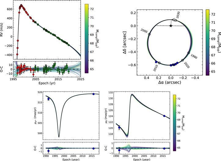
Figure 14. Results from a joint fit to host star radial velocity (top left), relative astrometry (top right), and absolute astrometry (bottom panel) for the HD 4747 system. The data together constrain the orbital parameters and mass of both the companion and host star well (Table 1).
Download figure:
Standard image High-resolution imageAppendix B: Extracted Low-resolution Spectrum and GPI Astrometry
Our extracted spectrum for HD 4747 B based on observations with GPI (Crepp et al. 2018) and SPHERE (Peretti et al. 2019) are given in Table 4. Our relative astrometry measurements based on the GPI data are listed in Table 5.
Table 4. Extracted Low-resolution Spectrum for HD 4747 B
| Wavelength (μm) | Flux (10−15 × W m−2/μm) | Flux Error (10−15 × W m−2/μm) |
|---|---|---|
| SPHERE (YJH) | ||
| 1.008 | 0.726 | 0.167 |
| 1.026 | 0.789 | 0.131 |
| 1.044 | 0.767 | 0.088 |
| 1.063 | 0.806 | 0.085 |
| 1.081 | 0.839 | 0.086 |
| 1.098 | 0.88 | 0.073 |
| 1.116 | 0.848 | 0.071 |
| 1.138 | 0.823 | 0.059 |
| 1.159 | 0.907 | 0.056 |
| 1.176 | 1.006 | 0.061 |
| 1.194 | 1.114 | 0.054 |
| 1.212 | 1.213 | 0.05 |
| 1.23 | 1.33 | 0.049 |
| 1.248 | 1.338 | 0.06 |
| 1.267 | 1.378 | 0.061 |
| 1.285 | 1.389 | 0.06 |
| 1.302 | 1.33 | 0.063 |
| 1.318 | 1.188 | 0.051 |
| 1.33 | 1.106 | 0.061 |
| 1.34 | 0.875 | 0.077 |
| 1.358 | 0.506 | 0.086 |
| 1.399 | 0.482 | 0.106 |
| 1.418 | 0.596 | 0.078 |
| 1.432 | 0.598 | 0.053 |
| 1.447 | 0.668 | 0.042 |
| 1.463 | 0.725 | 0.033 |
| 1.479 | 0.741 | 0.034 |
| 1.495 | 0.788 | 0.038 |
| 1.511 | 0.912 | 0.036 |
| 1.526 | 0.987 | 0.036 |
| 1.54 | 1.059 | 0.038 |
| 1.553 | 1.117 | 0.038 |
| 1.568 | 1.179 | 0.04 |
| 1.582 | 1.217 | 0.04 |
| 1.599 | 1.266 | 0.044 |
| 1.613 | 1.235 | 0.041 |
| GPI (H) | ||
| 1.506 | 0.789 | 0.022 |
| 1.51 | 0.798 | 0.022 |
| 1.516 | 0.841 | 0.024 |
| 1.522 | 0.89 | 0.025 |
| 1.531 | 0.936 | 0.026 |
| 1.539 | 0.983 | 0.028 |
| 1.547 | 1.046 | 0.031 |
| 1.554 | 1.107 | 0.031 |
| 1.562 | 1.153 | 0.032 |
| 1.572 | 1.183 | 0.033 |
| 1.581 | 1.218 | 0.033 |
| 1.589 | 1.233 | 0.034 |
| 1.597 | 1.22 | 0.033 |
| 1.605 | 1.216 | 0.032 |
| 1.613 | 1.21 | 0.031 |
| 1.621 | 1.201 | 0.032 |
| 1.63 | 1.21 | 0.033 |
| 1.638 | 1.208 | 0.032 |
| 1.646 | 1.183 | 0.031 |
| 1.654 | 1.181 | 0.032 |
| 1.662 | 1.18 | 0.032 |
| 1.67 | 1.172 | 0.033 |
| 1.678 | 1.171 | 0.033 |
| 1.686 | 1.153 | 0.032 |
| 1.695 | 1.143 | 0.031 |
| 1.703 | 1.126 | 0.03 |
| 1.711 | 1.084 | 0.029 |
| 1.719 | 1.05 | 0.028 |
| 1.727 | 1.007 | 0.027 |
| 1.735 | 0.949 | 0.025 |
| 1.743 | 0.878 | 0.023 |
| 1.751 | 0.818 | 0.022 |
| 1.758 | 0.759 | 0.021 |
| 1.765 | 0.693 | 0.019 |
| 1.772 | 0.63 | 0.017 |
| 1.777 | 0.57 | 0.018 |
| 1.781 | 0.525 | 0.015 |
| GPI (K1) | ||
| 1.892 | 0.547 | 0.063 |
| 1.898 | 0.627 | 0.054 |
| 1.905 | 0.608 | 0.081 |
| 1.907 | 0.671 | 0.032 |
| 1.916 | 0.654 | 0.026 |
| 1.924 | 0.624 | 0.02 |
| 1.932 | 0.588 | 0.019 |
| 1.941 | 0.567 | 0.019 |
| 1.95 | 0.559 | 0.018 |
| 1.96 | 0.561 | 0.019 |
| 1.969 | 0.582 | 0.02 |
| 1.977 | 0.582 | 0.018 |
| 1.985 | 0.561 | 0.018 |
| 1.993 | 0.564 | 0.018 |
| 2.003 | 0.633 | 0.018 |
| 2.016 | 0.694 | 0.021 |
| 2.025 | 0.693 | 0.022 |
| 2.033 | 0.692 | 0.022 |
| 2.041 | 0.697 | 0.022 |
| 2.049 | 0.727 | 0.022 |
| 2.059 | 0.759 | 0.023 |
| 2.069 | 0.762 | 0.025 |
| 2.077 | 0.772 | 0.027 |
| 2.086 | 0.744 | 0.022 |
| 2.094 | 0.752 | 0.023 |
| 2.103 | 0.764 | 0.028 |
| 2.111 | 0.79 | 0.024 |
| 2.12 | 0.79 | 0.028 |
| 2.129 | 0.778 | 0.028 |
| 2.138 | 0.787 | 0.024 |
| 2.147 | 0.771 | 0.025 |
| 2.155 | 0.749 | 0.022 |
| 2.163 | 0.728 | 0.021 |
| 2.17 | 0.695 | 0.022 |
| 2.176 | 0.662 | 0.023 |
| 2.181 | 0.615 | 0.022 |
| 2.183 | 0.471 | 0.025 |
Table 5. Extracted GPI Astrometry for HD 4747 B
| Time (BJD) | Separation (arcsec) | Position Angle (deg) |
|---|---|---|
| 2457380.5 | 0.5989 ± 0.002 | 183.9 ± 0.2 |
| 2457381.5 | 0.5984 ± 0.002 | 183.5 ± 0.2 |
Download table as: ASCIITypeset image
Appendix C: Priors and Posteriors for Retrieval Parameters
We list the priors on our retrieved parameters in Table 6 and include joint posterior distributions of selected parameters from our baseline HRS and LRS retrievals in Figures 15 and 16.
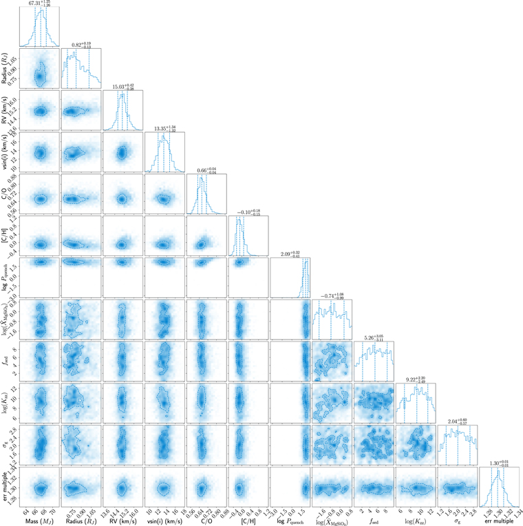
Figure 15. Joint posterior distributions for the HRS retrieval of HD 4747 B. We omit the P–T profile parameters, which are better visualized by the P–T plot in Figure 6.
Download figure:
Standard image High-resolution image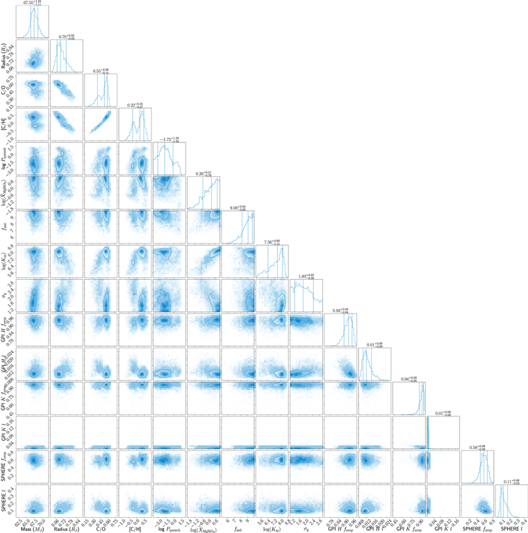
Figure 16. Joint posterior distributions for the LRS retrieval of HD 4747 B. We omit the P–T profile parameters, which are better visualized by the P–T plot in Figure 6. The distributions for a few parameters are bimodal.
Download figure:
Standard image High-resolution imageTable 6. Priors of the HD 4747 B Retrieval
| Parameter | Prior | Parameter | Prior |
|---|---|---|---|
| Mass (MJup) |

| C/O |

|
| Radius (RJup) |

| [Fe/H] |

|
| T1 (K) |

|

|

|
| T2 (K) |

| fsed |

|
| T3 (K) |

|

|

|
| Tint (K) |

| σg |

|
| α |

|

|

|

|
![${P}_{\mathrm{phot}}\in {\left[{10}^{-3},100\right]}^{({\rm{b}})}$](https://content.cld.iop.org/journals/0004-637X/937/2/54/revision1/apjac8673ieqn84.gif)
|

|

|
| Additional parameters for HRS | |||
| RV (km s−1) |

|
 (km s−1) (km s−1) |

|
| Error multiple |

| Flux scale (counts) |

|
| Gaussian process parameters for LRS | |||

|

|
 (μm) (μm) |

|
| Mass fraction of molecules | |||
| log(MMR) |

| ||
Note.  stands for a uniform distribution, with two numbers representing the lower and upper boundaries.
  stands for a Gaussian distribution, with numbers representing the median and standard deviation. (a) and (b): these priors follow Mollière et al. (2020). Pphot is the pressure where τ = 1, and Tconnect is the uppermost temperature of the “photospheric” layer, and is computed by setting τ = 0.1 in the Eddington Approximation (see Equations (1) and (2) in Mollière et al. 2020). This prior, along with those on T1 and T2 are used to prevent temperature inversions. (c)
  represents the scaling factor for the cloud mass fraction, so that
  refers to a fraction equal to the equilibrium mass fraction. fsed, Kzz, and σg are parameters in the EddySed cloud model (Ackerman & Marley 2001). When fitting molecular abundances directly (e.g., in Section 5.4), we use the same mass fraction prior on all molecules included.
Download table as: ASCIITypeset image
Footnotes
- 18
We will use HRS to abbreviate both high-resolution spectroscopy (the technique) and high-resolution spectrum (the data) in this paper. The same is true for LRS, low-resolution spectrum or spectroscopy.
- 19
- 20
- 21
- 22
- 23
We denote the atmospheric metallicity as [C/H] because we are only sensitive to C- and O-bearing molecules in this brown dwarf’s atmosphere.