Abstract
We test the predictions of the Alfvén Wave Solar Model (AWSoM), a global wave-driven magnetohydrodynamic (MHD) model of the solar atmosphere, against high-resolution spectra emitted by the quiescent off-disk solar corona. AWSoM incorporates Alfvén wave propagation and dissipation in both closed and open magnetic field lines; turbulent dissipation is the only heating mechanism. We examine whether this mechanism is consistent with observations of coronal EUV emission by combining model results with the CHIANTI atomic database to create synthetic line-of-sight spectra, where spectral line widths depend on thermal and wave-related ion motions. This is the first time wave-induced line broadening is calculated from a global model with a realistic magnetic field. We used high-resolution SUMER observations above the solar west limb between 1.04 and 1.34 R⊙ at the equator, taken in 1996 November. We obtained an AWSoM steady-state solution for the corresponding period using a synoptic magnetogram. The 3D solution revealed a pseudo-streamer structure transversing the SUMER line of sight, which contributes significantly to the emission; the modeled electron temperature and density in the pseudo-streamer are consistent with those observed. The synthetic line widths and the total line fluxes are consistent with the observations for five different ions. Further, line widths that include the contribution from the wave-induced ion motions improve the correspondence with observed spectra for all ions. We conclude that the turbulent dissipation assumed in the AWSoM model is a viable candidate for explaining coronal heating, as it is consistent with several independent measured quantities.
1. Introduction
The heating of the solar corona is one of the longest-standing and complex problems in solar physics. Coronal plasmas reach temperatures of 1–2 MK and more, and are thus several orders of magnitude hotter than the underlying chromosphere (∼50,000 K) and photosphere (∼5700 K). Thus, the energy responsible for heating the corona flows up from the Sun in a direction opposite the temperature gradient, implying that it cannot be transported by a thermal transport mechanism such as convection, conduction, or radiation. The mechanism that is responsible for coronal heating is yet to be identified conclusively. Current theoretical models of coronal heating and wind acceleration can be divided, broadly speaking, into two types: reconnection and wave-heating models (see Klimchuk 2006; Antiochos et al. 2011). In this work, we explore the wave-heating picture, and specifically the scenario in which Alfvén waves are the energy source and conduit driving coronal heating. It has been shown analytically that Alfvén waves are capable of heating the corona through wave dissipation (Barnes 1968, 1969) and accelerating the solar wind through the action of wave pressure (Alazraki & Couturier 1971; Belcher 1971). These hypotheses are supported by the observations that (1) Alfvénic perturbations are ubiquitous in the solar environment; they have been observed in the photosphere, chromosphere, coronal structures, and in the solar wind at Earth’s orbit (see Banerjee et al. 2011; McIntosh et al. 2011), and (2) the energy flux of Alfvén waves emanating from the chromosphere is sufficiently large to account for both coronal heating and solar wind acceleration (De Pontieu et al. 2007; McIntosh & De Pontieu 2012). However, for a complete picture of wave heating, one must also explain how the non-thermal wave energy will be converted into the thermal energy of coronal plasma. In other words, we must specify a wave dissipation mechanism. As of yet, an Alfvén wave dissipation mechanism responsible for coronal heating has not been conclusively identified. Several theoretical models of dissipation have been suggested, including phase mixing (Heyvaerts & Priest 1983), turbulent cascade (Matthaeus et al. 1999), and resonant absorption (Goossens et al. 2011). These models differ in the underlying physics as well as in the dissipation rates and length scales they predict. Ideally, these theories should be tested observationally, by comparing predicted and observed wave spectra, dissipation rates, and heating rates. However, direct and conclusive observational evidence for a specific dissipation model have not yet been obtained. This is largely because information about wave amplitudes in the corona is hard to extract, due to two uncertainties inherent in the observations. First, the observations are made remotely, and different regions along the line of sight of the detector can contribute to the detected emission. As a result, any measured quantity should be interpreted as a line-of-sight-integrated quantity. Second, wave amplitudes are observationally derived from measuring the widths of spectral lines. As we describe below in detail, this is because waves induce periodic motions of ions along the line of sight, giving rise to Doppler broadening of spectral lines. However, line broadening in the corona is not only due to waves, and can in fact be produced by simple thermal motions. Determining the unique contribution of waves to the observed line widths requires the aid of some model. One major goal of this work is to mitigate these uncertainties, at least partially, and perform detailed comparisons of predicted and observed wave amplitudes and plasma heating. The present study will attempt to test a specific model of wave dissipation, namely, the turbulent cascade. This mechanism has been studied extensively in the context of both the corona and the wind (e.g., Hollweg 1986; Matthaeus et al. 1999; Suzuki 2006; Cranmer et al. 2007; van Ballegooijen et al. 2011, to name a few), and it produces a unified treatment of all regions in the corona, which can be easily incorporated into a global model of the corona. We note that our approach is not designed to distinguish which of the different dissipation mechanisms is more viable; rather, we wish to test the general viability of Alfvénic energy as a conduit of non-thermal energy from the chromosphere into the different magnetic regions in the corona, by checking whether they produce plasma temperatures and wave amplitudes that are consistent with the observations. However, this work is intended to bring us one step further into determining whether (1) a sufficient portion of the energy contained in Alfvén waves at the top of the transition region an be transported into different regions of the corona, enough to heat the plasma to observed temperatures, and (2) wave dissipation can describe the conversion of wave energy into heat such that the partition between plasma thermal energy and remaining wave energy, at different heights above the chromosphere, are simultaneously consistent with observations. To answer these questions, we will use our theoretical model results to produce predictions that can be compared with the emission coming from the hot corona.
Extreme Ultraviolet (EUV) emission by heavy ions provides us with critical tools to study the physical processes taking place in the corona. For ions heavier than helium, coronal abundances are low. As a result they do not affect the overall dynamics, but nevertheless their emission in selected spectral lines can be routinely observed by dedicated space-based telescopes. An observed emission line can be characterized by the total energy flux (or “line flux”), and a line width, i.e., a range of wavelengths associated with the line, usually assumed to have a Gaussian shape around the central wavelength. The total line flux depends mainly on the electron density and temperature of the emitting plasma, while the line width is related to the state of the ions responsible for the emission. Specifically, unresolved ion motions along the line of sight will give rise to Doppler broadening and a larger line width. There are two mechanisms that dominate line broadening in the solar corona: thermal ion motions (due to their finite temperature) and non-thermal ion motions. Non-thermal motions of coronal ions may be due to transverse Alfvén waves (e.g., Hassler et al. 1990; Banerjee et al. 1998, 2009; Doyle et al. 1998; Moran 2001). McIntosh & De Pontieu (2012) have reported on observational evidence that non-thermal line broadenings are correlated with Alfvénic oscillations. Non-thermal line broadening may also be associated with high-speed flows taking place in nano-flares (Patsourakos & Klimchuk 2006). In this work, we study spectral lines formed in the quiet Sun, and therefore we do not address the contribution of this mechanism to the line width. Measuring non-thermal mass motions is a difficult endeavor, since both ion temperatures and non-thermal motions contribute to the observed line width and therefore some assumptions need to be made on the former in order to measure the latter (see Phillips et al. 2008 and references therein). Hahn et al. (2012) and Hahn & Savin (2013) studied the observed line broadening in a coronal hole and found evidence of wave damping. Despite many efforts, direct observational evidence of wave damping in the equatorial corona remain inconclusive. This may be attributed to line-of-sight effects, whereby different spectral lines are actually emitted from different regions.
Several numerical models were aimed at simulating Alfvénic perturbations in the solar corona and predicting the observed non-thermal motions. Ofman & Davila (1997) generated Alfvén waves in a 2.5D resistive magnetohydrodynamic (MHD) model of an idealized coronal hole. In Ofman & Davila (2001) and Ofman (2004) this work was extended to a multi-fluid description in order to directly simulate the motions of the emitting ion species due to a broadband Alfvén wave spectrum injected at the base. They directly calculated the resulting line broadening and found it to agree well with observations. Dong & Singh (2013) have presented results from test-particle simulations showing that a Maxwellian distribution of ion speeds will be broadened when subjected to Alfvén waves. They found that the Maxwellian shape is more likely to be preserved during this process when acted on by a wave spectrum, compared to a monochromatic wave. Matsumoto & Suzuki (2014) performed 2.5D MHD simulations, where they did not invoke dissipation explicitly, but rather allowed it to evolve self-consistently from the perturbations. Their predicted coronal temperatures and wave amplitudes in a slab of coronal plasma were consistent with observations. Although these efforts allowed for a detailed description of wave-induced motions, they were restricted to prescribed and idealized magnetic fields. In this work, we wish to extend these efforts to a global model, in which the magnetic field evolves self-consistently with the plasma and wave field, and whose topology can be derived from synoptic maps of the photospheric magnetic field. This allows us to predict EUV line widths and compare them to observations at any location in the lower corona.
Several MHD models based on synoptic maps have been developed (Usmanov 1993; Linker et al. 1999; Mikić et al. 1999; Roussev et al. 2003; Riley et al. 2006; Cohen et al. 2007). These earlier models employed geometric or empirical terms in the plasma energy equation in order to mimic the observed plasma heating and wind acceleration rates. Evans et al. (2008) found that the radial profiles of the Alfvén speed predicted by models using empirical/geometric terms in the energy equation were in general less consistent with the observed profiles compared to idealized wave-driven models. In addition, these global MHD models have set their lower boundary at the already hot (∼1 MK) corona and did not describe the formation of the hot corona from the much cooler chromosphere. Lionello et al. (2009) and Downs et al. (2010) were the first global models to set the inner boundary at the top of the chromosphere. They were able to reproduce the large-scale features of the lower corona as observed in full-disk EUV images by applying different geometric heating functions in coronal holes, streamer belts, and active regions. However, models based on empirical heating functions are limited by the fact that the energy source itself does not evolve self-consistently with the plasma. A more self-consistent description of heating and acceleration can be achieved within the framework of MHD by including the effects of Alfvén waves, which can exchange energy and momentum with the plasma through wave dissipation and wave pressure gradients, respectively (Jacques 1977). Alfvén waves were first included in a 3D MHD model of the solar corona in Usmanov et al. (2000) and later in Usmanov & Goldstein (2003), assuming an ideal dipole magnetic field. These models solved the MHD equations coupled to the wave kinetic equation for low-frequency Alfvén waves of a single polarity undergoing linear dissipation. A more sophisticated treatment of the dissipation mechanism was implemented in the global model of van der Holst et al. (2010), which assumed that a Kolmogorov-type nonlinear dissipation is taking place in open field line regions, based on the description proposed in Hollweg (1986); no waves were present in closed field lines. This model was validated in Jin et al. (2012), and later extended to include surface Alfvén waves in Evans et al. (2012). However, the inner boundary of this model was set at the bottom of the corona with temperatures in the ∼1 MK range, thus avoiding the problem of forming the corona from the much cooler chromosphere.
In this work, we use the Alfvén Wave Solar Model (AWSoM; Oran et al. 2013; Sokolov et al. 2013; van der Holst et al. 2014), a global model of the solar atmosphere driven by Alfvén wave energy, which is propagated and dissipated in both open and closed magnetic field lines. The model extends from the top of the chromosphere and up to 1–2 au and thus addresses both coronal heating and formation of the solar wind. The interaction of the plasma with the wave field is described by coupling the extended-MHD equations to the wave kinetic equations of low-frequency Alfvén waves propagating parallel and anti-parallel to the magnetic field. Wave dissipation due to a turbulent cascade is the only heating mechanism assumed in the model. The wave energy in this description represents the time average of the perturbations due to a turbulent spectrum of Alfvén waves. Relating this energy to the non-thermal line broadening and combining the 3D model results with a spectroscopic database, we are able to calculate synthetic emission line profiles integrated along the entire line of sight. The synthetic spectra are used in two ways. First, we compare the synthetic line widths to observations in order to test the accuracy of the model predictions of the Alfvén wave amplitude and ion temperatures. Second, the synthetic and observed total line fluxes are compared in order to test the accuracy of the model predictions of electron density and temperature. In addition, we directly compare the model electron density and temperature to remote measurements based on line intensity ratios. For this purpose, we perform a careful analysis of the emission along the SUMER line of sight as predicted by the model in order to locate the region that is responsible for the relevant line emission.
This series of independent observational tests allows us to examine whether we can simultaneously account for the coronal plasma heating rate, together with the amount of remaining (non-dissipated) wave energy. Such a comparison provides a vital benchmark for the scenario where coronal heating is due to Alfvén wave dissipation. To the best of our knowledge, this is the first time that observed non-thermal mass motions are used to test the heating mechanism in a three-dimensional global model. In the particular case of the AWSoM model, an agreement between the model results and observations would suggest that both the amount of wave energy injected into the system (i.e., the Poynting flux from the chromosphere) and the rate at which the wave energy dissipates at higher altitudes are consistent with observations. A good agreement between the synthetic and observed quantities would suggest that the form of wave dissipation assumed in the model is a viable candidate for describing the transport of Alfvén waves in the solar atmosphere.
In order to make meaningful comparisons to observations, we require high-quality, and high spatial and high spectral resolution data. We selected a set of observations carried out by the Solar Ultraviolet Measurements of Emitted Radiation (SUMER) instrument on board the Solar and Heliospheric Observatory (SoHO; Wilhelm et al. 1995) during 1996 November 21–22, in which the SUMER slit was oriented along the solar east–west direction and the SUMER field of view stretched radially from 1.04 to 1.34 solar radii outside the west limb. The AWSoM model was used to create a steady-state simulation for Carrington Rotation 1916 (CR 1916; 1996 November 11–December 9), from which we produced synthetic spectra in selected SUMER lines. The radial orientation of the slit allows us to compare predicted and observed quantities as a function of distance from the limb.
This paper is organized as follows. In Section 2, we discuss the thermal and non-thermal line broadening of optically thin emission lines. In Section 3, we briefly describe the AWSoM model and the numerical simulation for CR 1916. The observations used in this study are introduced in Section 4. We describe the method of creating synthetic emission line profiles in Section 5. Section 6 reports on the resulting line profiles and their comparison to observations; the comparison of the model results to the electron density and temperature diagnostics is also shown, and the wave dissipation in the observed region is analyzed. We discuss the results and their implications in Section 7.
2. Thermal and Non-thermal Line Broadening
Unresolved thermal and non-thermal motions of ions will cause emission lines associated with these ions to exhibit Doppler broadening. Outside active regions, the resulting line profile can be approximated by a Gaussian, whose width depends on both the thermal and non-thermal speeds. In the most general case where the non-thermal motions are assumed to be random, the observed FWHM of an optically thin emission line will be given by (Phillips et al. 2008)
where  is the instrumental broadening,
  is the rest wavelength, c is the speed of light, kB is the Boltzmann constant, Ti and Mi are the temperature and atomic mass of ion i, respectively, and vnt is the non-thermal speed along the line of sight. It is evident from Equation (1) that one cannot determine the separate contributions of thermal and non-thermal motions from the observed FWHM alone. Instead, one must either make some assumption about the ion temperatures or use some model that describes and predicts the magnitude of vnt. In this work, we take a different approach, in which we predict both the ion temperatures, Ti, and the non-thermal speed, vnt at every location along the line of sight from a global model of the solar atmosphere, and compare the resulting spectra to observations. For this purpose, we assume that the non-thermal motions of coronal ions are due to transverse Alfvén waves, which cause the ions to move with a velocity equal to the wave velocity perturbation,
  . In this case, the non-thermal speed can be determined according to (Hassler et al. 1990; Banerjee et al. 1998)

where  denotes an average over timescales much larger than the wave period, and α is the angle that the plane perpendicular to the magnetic field makes with the line-of-sight vector. Equation (2) shows that the non-thermal speed is related to the root mean square (rms) of the velocity perturbation rather than to the instantaneous vector. This is due to the fact that line broadening is associated with unresolved motions whose periods are much smaller than the integration time of the detector. The dependence on α reflects the fact that the non-thermal motions due to Alfvén waves are inherently anisotropic. The vector
  lies in a plane perpendicular to the background magnetic field, and only its component along the line of sight contributes to the Doppler broadening of the emission. This dependence on the magnetic field topology is often neglected in works involving coronal holes, but it must be taken into account when considering the equatorial solar corona.
The quantity  can be calculated from a wave-driven model of the solar corona, which describes self-consistently the evolution of the wave field coupled to an MHD plasma. In order to calculate the ion temperatures in detail, one in principle should use a multi-species/multi-fluid MHD description (e.g., Ofman & Davila 2001; Ofman 2004). Such an approach to a global model of the solar atmosphere is quite involved and is beyond the scope of the present work. However, an extended-MHD description that includes separate electron and proton temperatures might be sufficient, if one assumes that the ions are in thermodynamic equilibrium with the protons. This assumption can be reasonable in the equatorial lower corona due to the high density. Thus, a model that allows the calculation of both the wave amplitude and the proton temperature should be capable of predicting the line broadening under the assumptions we just stated.
3. Wave-driven Numerical Simulation
3.1. AWSoM Model Description
The Alfvén Wave Solar Model (AWSoM) is a global, wave-driven, extended-MHD numerical model starting from the top of the chromosphere and extending into the heliosphere beyond Earth’s orbit. The waves drive the model by exchanging momentum and energy with the plasma: gradients in the wave pressure accelerate the plasma, while dissipation converts wave energy into thermal energy. Wave dissipation is the only explicit heating mechanism invoked, and no ad hoc or geometric heating functions are included. The time and spatial scales associated with the wave phenomena are much smaller than the characteristic scales of the entire system, making it impractical to resolve the wave motions in a global model. We therefore adopt an approach where the wave energy evolves according to wave kinetic equations under the WKB approximation. Two such equations, for low-frequency Alfvén waves propagating parallel and anti-parallel to the magnetic field, are coupled to the MHD equations.
The model is based on BATS-R-US (Tóth et al. 2012), a versatile, massively parallel MHD code with adaptive mesh refinement. The computational domain used in this work is a non-uniform spherical grid which allows us to treat the sharp gradients in the transition region as well as resolve the heliospheric current sheet. AWSoM is implemented within the Space Weather Modeling Framework (SWMF; Tóth et al. 2012).
3.2. Governing Equations
The model equations are based on the two-temperature MHD equations derived in Braginskii (1965), with the following simplifications: the Hall effect is neglected, and the electrons and protons are assumed to have the same bulk velocity. This leads to single-fluid continuity and momentum equations, and separate pressure equations for electrons and protons. The latter allow us to incorporate non ideal-MHD processes such as electron heat conduction, radiative cooling, and electron−proton heat exchange. The extended-MHD equations are coupled to wave kinetic equations for parallel and anti-parallel waves, as described in Sokolov et al. (2009), van der Holst et al. (2010), and Sokolov et al. (2013). The governing equations then become


These equations describe the evolution of the mass density, ρ; the bulk flow velocity,  ; the magnetic field,
  ; and the proton and electron thermal pressures, pp and pe, respectively.
  is the energy density of Alfvén waves propagating parallel (+) or anti-parallel (−) to the magnetic field. Next, G is the gravitational constant,
  is the solar mass,
  is the magnetic permeability, and γ is the polytropic index set to be constant at 5/3. The Alfvén velocity is given by
  . The pressure tensor due to Alfvén waves is given by
  (see, e.g., Jacques 1977).
The wave kinetic equations are given in Equation (6), which represents two separate equations, for the two wave polarities. The wave energy density dissipation rate of the two wave modes is denoted by  . The total wave energy density dissipation rate is given by
  . The pressure equations for protons and electrons are given in Equations (7) and (8), respectively. The dissipated wave energy is partitioned between the two species, where the fraction heating the protons is denoted by fp, which is set at 0.6 (see Cranmer et al. 2009; Breech et al. 2009). The radiative cooling rate of the electrons, Qrad, represents the loss of energy due to emission from the plasma at a given location. The emission is assumed to be due to electronic de-excitation, which is important in the cooler chromosphere to the lower corona, and becomes negligible in the 1 MK hot corona. The cooling rates are calculated from the CHIANTI 7.1 atomic database (Dere et al. 1997; Landi et al. 2013). The ion population responsible for the radiation is calculated by assuming coronal elemental abundances as reported in Feldman et al. (1992) and ionization equilibrium (due to the ionization and recombination rates appearing in Landi et al. 2013).
Heat exchange due to Coulomb collisions between electrons and protons enters the energy equations through the second term on the right-hand side of both equations. The collisional heat exchange results in temperature equilibration on a timescale  , which is given by (Goedbloed & Poedts 2004)
where mp and me are the proton and electron masses, respectively, e is the elementary charge, k is the Boltzmann constant, Te is the electron temperature,  is the permittivity of free space, n is the plasma number density (under the assumption of quasi-neutrality), and
  is the Coulomb logarithm, taken to be uniform with
  . Since the thermal coupling between the two species is proportional to the plasma density, it becomes negligible as the density drops off with distance from the Sun. The electron energy equation, Equation (8), includes the field-aligned thermal conduction tensor, denoted here by
  and given by the Spitzer form.
3.3. Wave Heating
The model assumes that a Poynting flux of Alfvén waves propagates through the top of the chromosphere, with a magnitude proportional to the local magnetic field and constrained by observations (see Table 1). The polarity of the wave emitted from each point on the inner boundary is determined by the direction of the local radial magnetic field. The wave energies of the two wave polarities evolve self-consistently with the plasma according to Equations (6)–(8). This allows us to directly account for the effects of wave pressure on the flow. However, a physics-based description of the wave dissipation requires us to consider the evolution of the wave spectrum, an approach that would essentially make a global model four dimensional (as was discussed in Sokolov et al. 2009; Oran et al. 2010). An alternative to this approach is to adopt a Kolmogorov-type dissipation rate, based on the assumption that the wave energy represents an average over a turbulent spectrum, and that it dissipates due to a fully developed turbulent cascade (Matthaeus et al. 1999). This approach, first presented in Hollweg (1986) for open magnetic field lines, allows one to treat the effects of wave dissipation although the detailed microphysical processes are not simulated explicitly. Further, by incorporating a Kolmogorov-type dissipation term into the coupled system of wave-transport and MHD equations, we can achieve a self-consistent description that is based on sound physical arguments while still accounting for the unresolved evolution of the wave field. A self-consistent heating mechanism is a major step forward compared to coronal models that employ geometric or fully empirical heating functions in the MHD equations, because the heating source is itself evolving. The present model employs the wave dissipation term presented in Sokolov et al. (2013), who generalized the Hollweg (1986) approach treating wave dissipation in both open and closed magnetic field lines. The resulting dissipation rate allows the boundary between the open and closed field lines to evolve self-consistently. This mechanism was analyzed in detail in Oran et al. (2013) and shown to be equivalent to the dissipation terms invoked in Matthaeus et al. (1999) and Cranmer et al. (2007). Further, the modeled thermal structure in the lower corona was validated against full-disk EUV images, while the flow properties of the wind at 1–2 au were validated against Ulysses observations. Further validation of the thermal and flow structure at the lower corona was presented in Landi et al. (2014), where the model performance was compared to other coronal models (for an ideal dipole magnetic field case), and in Oran et al. (2015), who showed that the modeled electron density and temperature are consistent with differential emission measure tomography of the lower corona (for another solar minimum case). As for comparing the simulated wave transport to observations, it was shown in Oran et al. (2013) that the modeled wave amplitudes were consistent with observations taken from the lower corona and up to 1 au along open polar magnetic field lines during solar minimum. In this work, we wish to extend this comparison by focusing on the equatorial lower corona, producing synthetic spectra, and comparing them to detailed spectroscopic observations of line broadening. We will thus be able to study how well the turbulent cascade dissipation assumed here reproduces the observations, and to make the first (to our knowledge) comparison of modeled and observed emission line broadening due to Alfvén waves propagating and dissipating in a realistic coronal magnetic field.
Table 1. Input Parameters and Inner Boundary Values for the AWSoM Steady-state Simulation for CR 1916
| Input Parameter | Value |
|---|---|
 a
a
|
25 kma |

|
0.06 |
| Poynting flux per unit Bb |

|
| Base electron temperature, Te | 50,000 K |
| Base proton temperature, Tp | 50,000 K |
| Base electron density, ne |

|
| Base proton density, np |

|
Notes.
aThe correlation length, , in Equation (10) is determined by
 ![${L}_{\perp }={L}_{\perp ,0}\sqrt{1[T]/B[T]}$](https://content.cld.iop.org/journals/0004-637X/845/2/98/revision1/apjaa7fecieqn27.gif) , where
, where ![$[T]$](https://content.cld.iop.org/journals/0004-637X/845/2/98/revision1/apjaa7fecieqn28.gif) denotes a magnetic field measured in units of Tesla.
bThis value is based on the Hinode observations reported in De Pontieu et al. (2007), and corresponds to an rms wave velocity amplitude,
denotes a magnetic field measured in units of Tesla.
bThis value is based on the Hinode observations reported in De Pontieu et al. (2007), and corresponds to an rms wave velocity amplitude,  km s−1, observed at an altitude where the plasma density is
  cm−3.
cm−3.
Download table as: ASCIITypeset image
The wave dissipation term used in this work is based on a phenomenological description of a fully developed turbulent cascade (Matthaeus et al. 1999). For the sake of brevity, we will not repeat the full derivation and justification of this term and refer the reader to Sokolov et al. (2013) and Oran et al. (2013) for a more detailed analysis. It is worthwhile, however, to describe this term and the adjustable parameters controlling it. The energy density dissipation,  , is given by
Note that the dissipation depends on the relative magnitudes of the two wave polarities, leading to different heating rates in open and closed field lines. This unified approach, presented in Sokolov et al. (2013), ensures that the spatial distribution of the coronal heating rates will emerge automatically and self-consistently with the magnetic field topology. A detailed analysis of this approach and its implications can be found in Oran et al. (2013). The total dissipated wave energy heats both protons and electrons, with the fraction of heating going into the protons denoted by the constant fp = 0.6 (see Breech et al. 2009; Cranmer et al. 2009 for more details). It is important to note that the model version and global simulation used here are those from Oran et al. (2013), and so reflections are not directly simulated by the model; rather, the pseudo-reflection coefficient  serves to mimic their effect under the assumption of a fully developed turbulent cascade. In this approximation, any wave energy created by reflections is dissipated locally by the cascade process before it can be carried away by the reflected wave (Matthaeus et al. 1999; Dmitruk & Matthaeus 2003; Cranmer et al. 2007; Chandran & Hollweg 2009). Thus, in practice there is no need to convert the outgoing wave energy into the opposite polarity, as the wave energy is converted into heat. A less restrictive treatment that includes a self-consistent description of wave reflections in a global model was implemented in van der Holst et al. (2014). The dissipation mechanism is controlled by two adjustable parameters: a constant pseudo-reflection coefficient,
  , and the transverse correlation length for Alfvénic turbulence, L⊥, which varies with the width of the magnetic flux tube such that
  (Hollweg 1986).
3.4. Relating the Non-thermal Speed to the Modeled Wave Energy
In the AWSoM model, the wave energy evolves under the WKB approximation. The perturbations due to Alfvén waves propagating parallel and anti-parallel to the background magnetic field can be conveniently described by the Elsässer fluctuation variables (Tu & Marsch 1994), defined as 
 , where
  and
and  are the velocity and magnetic field perturbations, respectively, and
  is the permeability of free space. The energy densities of non-compressible Alfvén waves can be expressed as
  , while the square of the velocity perturbation can be obtained from
On open field lines, only one wave polarity should dominate if the reflection is negligible so that the product  will be zero. On closed field lines, opposite wave polarities are injected at the two footpoints of the field line, giving rise to counter-propagating waves. However, in the balanced turbulent regime near the top of the closed field lines, these perturbations are presumed to be uncorrelated:
  . Thus, the last term on the right-hand side of Equation (11) will drop out in any magnetic topology. The square of the velocity perturbation now becomes
Combining Equations (2) and (12), we can relate the non-thermal speed to the wave energies as
Note that under the WKB approximation, the wave energy density is already an average over timescales much larger than the wave period, and there is no need for averaging.
3.5. Steady-state Simulation for Carrington Rotation 1916
In order to produce a realistic steady-state solution for the period during which the SUMER observations were taken, we derive the inner boundary conditions of the model using a synoptic line-of-sight magnetogram of the photospheric radial magnetic field, acquired during CR 1916 (lasting from 1996 November 11 to 1996 December 9). The magnetogram was obtained by the Michelson–Doppler Interferometer (MDI) instrument on board the SoHO spacecraft (Scherrer et al. 1995). In order to compensate for the reduced accuracy at the polar regions, we use a polar-interpolated synoptic magnetogram, provided by the Solar Oscillations Investigation (SOI) team (Sun et al. 2011). The resulting radial magnetic field is shown in Figure 1.
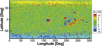
Figure 1. Boundary condition for the radial magnetic field for CR 1916, obtained from an MDI magnetogram with polar interpolation. Although the magnetic field magnitude can reach up to 2000 G in the vicinity of active regions, the color scale was modified so that the large-scale distribution can be seen.
Download figure:
Standard image High-resolution imageThe values used for the model’s adjustable parameters and inner boundary conditions for this simulation are listed in Table 1. The dissipation length and reflection coefficient are not unique, but may vary in a defined range that is empirically motivated and consistent with previous models, as explained in Sokolov et al. (2013) and Oran et al. (2013). Due to the high computational cost of global coronal models, it is not feasible to perform a complete sensitivity study of parameter space. Nonetheless, the specific values used here were chosen in Oran et al. (2013) under the constraint that the solution is capable of reproducing the observations both near the corona and far in the solar wind for a different solar minimum case. That simulation was validated against a myriad of observations from the lower corona to interplanetary space at 2 au in Oran et al. (2013, 2015). The use of the same values for two different Carrington Rotations during solar minimum is reasonable and does not introduce additional uncertainty. Indeed, the global solution reproduced the global structure of the corona well, as we demonstrate in Section 6.1.
4. Observations
The observations we used in this work were taken by the SUMER instrument on board SoHO on 1996 November 21–22. During this time, SoHO was rolled 90° so that the SUMER slit was oriented along the east–west direction. The center of the SUMER 4″ × 300″ slit was pointed at (0″, 1160″) so that the field of view stretched almost radially from 1.04 to 1.34 R⊙ lying outside the west solar limb at the solar equator. The entire 660–1500 Å wavelength range of SUMER detector B was telemetered down; given the particular instrumental configuration, this range was divided into 61 sections of 43 Å, each shifted from the previous one by ≈13 Å. Each section was observed for 300 s. More details on these observations can be found in Landi et al. (2002).
From the available spectral range, we chose a set of bright and isolated spectral lines (listed in Table 2), which allow accurate measurements of both line fluxes and line widths up to high altitudes. We note that the very bright O vi doublet at the 1031–1037 Å range was not selected because these lines are partially formed by radiative scattering from the photosphere, and thus their theoretical FWHM is more complex than given in Equation (1), making them inadequate for our purposes.
Table 2. Selected Emission Lines Used in This Study
| Ion Name | Wavelength (Å) | Rmax 
|
 (Å) (Å) |
|---|---|---|---|
| Fe xii | 1242.01 | 1.275 | 0.178 |
| S x | 1196.22 | 1.265 | 0.180 |
| Mg ix | 706.06 | 1.245 | 0.198 |
| Na ix | 681.70 | 1.285 | 0.199 |
| Ne viii | 770.41 | 1.255 | 0.196 |
Note. The first column shows the ion name, while the second column reports the central wavelength at r = 1.04 R⊙. The third column reports the highest altitude at which the observed flux is at least two times larger than the instrument-scattered flux (see Section 4.2). The fourth column reports the wavelength-dependent instrumental broadening for SUMER detector B, as given by the standard SUMER reduction software (see Section 5.2).
Download table as: ASCIITypeset image
4.1. Data Reduction
The data were reduced using the standard SUMER software made available by the SUMER team through the SolarSoft IDL package (Freeland & Handy 1998); each original frame was flat-fielded, corrected for geometrical distortions, and aligned with all other frames. In order to increase the signal-to-noise ratio, the data were averaged along the slit direction in 30 bins, each 0.01 R⊙ wide. Spectral line profiles were fitted with a Gaussian curve removing a linear background. The resulting count rates were then calibrated using the standard SUMER calibration also available in SolarSoft. The accuracy of the spectral flux calibration of SUMER detector B before 1998 June is ≈20% (Wilhelm 2006, and references therein).
4.2. Scattered Light Evaluation
The micro-roughness of the SUMER optics causes the instrument to scatter the radiation coming from the solar disk into the detector, even when the instrument is pointing outside the limb. The scattered light forms a ghost spectrum of the solar disk at rest wavelength superimposed onto the actual spectrum emitted by the region imaged by the SUMER slit.
This ghost spectrum can provide important, though undesired, contributions to measured line fluxes when the local emission of the Sun is weak; these contributions need to be evaluated and, when necessary, removed. Unfortunately, the strength of the ghost spectrum depends on a number of factors (slit pointing, strength of the disk spectrum etc.), which make it impossible to devise a procedure to automatically remove it from the observations; its estimation needs to be performed on a case-by-case basis.
In the case of the present observations, the almost radial pointing of the SUMER slit allows us to use the rate of decrease of spectral line intensities with distance from the limb in order to determine an upper limit on the contributions of the ghost spectrum. Since emission line intensities depend on the square of the electron density, the rapid decrease of the latter with height causes the coronal line intensities to decrease by almost two orders of magnitude from the closest to the farthest end of the slit in the present observation; in contrast, the scattered light intensity, which is not emitted by the plasma in the observed region, is only reduced by a factor  over the same range.
Landi (2007) devised a two-step method to determine an upper limit on the scattered light contribution to any spectral line for off-disk observations stretching over a large range of distances from the limb. First, the rate of decrease of the scattered light intensity with height is determined, based on several lines that are not emitted by the corona and whose off-disk intensity is entirely due to scattering. Second, the rate of decrease of the scattered light intensity is used to get an upper limit on its contribution to a specific coronal line as follows. We measure the intensity of the coronal line at the location farthest from the limb in the instrument’s field of view and assume that this intensity is entirely due to scattered light. The radial rate of decrease of the scattered light intensity is then normalized to match that coronal line intensity at the same height, giving an upper limit to the scattered light contribution at all other heights. Note that this method actually overestimates the scattered light contribution to coronal lines.
To estimate the radial rate of decrease of the scattered light intensity, we have used the intensity of the continuum at 1475 Å and of the following lines: He i 584 Å, C ii 1335 Å, C iii 977 Å, O i 1302 Å, 1304 Å and 1306 Å, O iii 835 Å, and Si iii 1206 Å. These lines and continuum are emitted by the solar chromosphere, so that they are expected to be too weak to be observed at the heights covered by the SUMER field of view: their observed intensity is entirely due to scattered light. The rate of decrease of each of these lines and continuum have been normalized to the value of the intensity at the largest distance from the limb and averaged together to provide the final scattered light intensity versus height curve. This curve appears as the light green curve in Figure 2. The normalized intensity versus height curve for the lines in Table 2 is also shown for comparison. We verified that all of them decreased at a rate much faster than the scattered light intensity: this suggests that the latter is at best a minor contributor to the intensity of each of the lines in Table 2. We also determined the maximum heliocentric distance Rmax below which the scattered light contribution to the coronal line intensity is less than 50%. We take this arbitrary limit as an indication of the range of heights where we can safely neglect the scattered light. This height is reported in the third column of Table 2. We note that all of the emission lines considered here possessed a clear Gaussian line shape that could be separated from the background up to distances larger than Rmax.
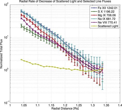
Figure 2. Rate of decrease of the intensity of coronal lines and scattered light as a function of radial distance. All curves are normalized to the scattered light intensity measured at r = 1.34 R⊙ (the farthest point of the SUMER slit). Colored curves correspond to the five lines in Table 2 and the averaged scattered light.
Download figure:
Standard image High-resolution image5. Synthesizing EUV Emission Line Profiles from 3D Model Results
The synthetic line profiles were calculated by combining the AWSoM model predictions of the plasma properties and wave energy with the spectral emissivity calculated from the CHIANTI 7.1 atomic database (Dere et al. 1997; Landi et al. 2013). CHIANTI takes into account known line formation mechanisms and is capable of calculating the total emission of a spectral line, given the electron density and temperature. The calculations included in this work were carried out assuming that the plasma is optically thin and in ionization equilibrium. Photo-excitation was neglected as a line formation mechanism.
5.1. Total Flux of Ion Emission Lines
The total line emission in a plasma volume, dV, having electron temperature Te and density Ne is given by

where  is the contribution function for a spectral line associated with an electronic transition from an upper level j to a lower level i, defined as
where Gji is measured in units of photons cm3 s−1. X+m denotes the ion of the element X at ionization state  . The contribution function also depends on the following quantities:
- 1.
 is the relative level population of ions at level j, and depends on the electron density and temperature;
 - 2. is the abundance of the ion relative to the abundance of the element X, and depends on the electron temperature;
- 3. is the abundance of the element X relative to hydrogen;
- 4. is the hydrogen abundance relative to the electron density (∼0.83 for fully ionized plasmas); and
- 5.Aji is the Einstein coefficient for the spontaneous emission for the transition.


As Te and Ne are known from the model solution, the contribution function in any computational volume element can be calculated. In this work, we used coronal element abundances as given in Feldman et al. (1992) and the latest ionization equilibrium computation available in CHIANTI (Landi et al. 2013).
Once the contribution function is calculated at every point along the line of sight, the total observed flux in the optically thin limit is given by integrating the emissivity along the line of sight:

where d is the distance of the instrument from the emitting volume dV. Ftot is measured in units of photons cm−2 s−1. This volume integral can be replaced by a line integral by observing that dV = Adl, where A is the area observed by the instrument and dl is the path length along the line of sight. In the case of the present observations, the area covered by the instrument is 4″ × 1″. In order to calculate the line-of-sight integral from the 3D model results, we interpolate Gji and Ne from the AWSoM non-uniform spherical computational grid onto a uniformly spaced set of points along each observed line of sight. The spacing used for the interpolation was set to match the finest grid resolution of the model. This procedure ensures that the integration is second-order accurate.
5.2. Synthetic Line-of-Sight-integrated Line Profiles
Knowledge of the magnitude of thermal and non-thermal ion motions allows us to calculate a synthetic spectrum, which explicitly includes their effects on the line profile. Thus, instead of merely predicting the total flux of an emission line, we can predict the full spectral line profile to be compared with the observed spectrum.
For each location along the line of sight, the local spectral flux can be calculated by imposing a Gaussian line profile characterized by the predicted total flux, Ftot, the rest wavelength  , and line width,
  , determined from the ion temperature and the magnitude of non-thermal motions. The spectral flux, measured in units of photons cm−2 s−1 Å−1, can be written as

where  is the normalized line profile. In the case of a Gaussian line profile,
  is given by
and the line width, in accordance with Equation (1), can be written as
The non-thermal speed, vnt, can be calculated from the AWSoM model through Equation (13). The emitting region in our case is a three-dimensional non-uniform plasma, where each plasma element along the line of sight gives rise to different values of the total flux and the line width. In order to synthesize the line profile from the model, we must perform the line-of-sight integration for each wavelength separately, i.e., we must calculate the spectral flux at the instrument,  , given by

The spectral flux is calculated over a wavelength grid identical to the SUMER spectral bins. In order to compare the synthetic spectra with observations, we must also take into account the SUMER instrumental broadening. For this purpose, we convolve the line-of-sight-integrated spectral flux with the wavelength-dependent instrumental broadening for SUMER detector B, as given by the standard SUMER reduction software available through the SolarSoft package.
5.3. Uncertainties in Atomic Data and Line Flux Calculations
Atomic data uncertainties directly affect the line fluxes calculated from the AWSoM simulation results. It is therefore necessary to discuss the accuracy of the data available for the emission lines for which we wish to produce synthetic spectra. Table 2 lists the five spectral lines that were used for detailed line profile calculations. They were chosen mainly because they are bright and clearly isolated from neighboring lines, so that their profile could be resolved accurately to as large a height as possible.
5.3.1. Ne viii 770.4 Å and Na ix 681.7 Å
These two lines belong to the Li-like iso-electronic sequence, i.e., they possess one bound electron in their outer shell. Their atomic structure is relatively simple, and the theoretical calculation of their collisional and radiative rates is expected to be accurate. Landi et al. (2002) verified the accuracy of this calculation for all lines belonging to this sequence by comparing the fluxes calculated from CHIANTI to those measured in the 1.04 R⊙ section of the observations used here. The authors used the electron density and temperature measured in that section as input to CHIANTI. They found excellent agreement among all lines of the sequence, indicating that the collisional and radiative rates are indeed accurate. However, they found a systematic factor of 2 overestimation of the abundance of all ions of this sequence, which they ascribed to inaccuracies in the ionization and recombination rates used in their work (from Mazzotta et al. 1998). However, more recent assessments of ionization and recombination rates made by Bryans et al. (2006, 2009) largely solved this discrepancy, as shown by Bryans et al. (2009). Since we are using ion abundances that take into account the new electron impact ionization by Bryans et al. (2009), the fluxes of these two lines are expected to be reasonably free of atomic physics problems.
5.3.2. Mg ix 706.0 Å
The CHIANTI calculation of the flux of this line was found to be in agreement with other lines from the same sequence by Landi et al. (2002); however, some problems were found with some other Mg ix lines observed by SUMER, making this ion a candidate for uncertainties in atomic data. However, the radiative and collisional transition rates used in the present work (from CHIANTI 7.1) have been improved from those used by Landi et al. (2002), which used CHIANTI 3 (Dere et al. 2001). The new calculations now available in CHIANTI, from Del Zanna et al. (2008), solved the problems so that the atomic data for this ion should be accurate.
5.3.3. S x 1196.2 Å
The atomic data of the S x 1196.2 Å line were also benchmarked by Landi et al. (2002), who showed that while all of the data in the N-like iso-electronic sequence were in agreement with each other, they all indicated a larger plasma electron temperature than the other sequences, suggesting that improvements in this sequence were needed. Subsequent releases of CHIANTI adopted larger and more sophisticated calculations for this ion, so that the accuracy of the predicted flux for S x 1196.2 Å should be relatively good. However, this line is emitted by metastable levels in the ground configuration, and its flux is strongly density sensitive. Thus, inaccuracies in the predicted electron density may result in large errors in the calculated line flux.
5.3.4. Fe xii 1242 Å
Fe xii has a complex electronic structure and therefore large atomic models are required to fully describe its wave functions. For example, when EUV lines emitted by this ion are used to measure the electron density, they are known to overestimate it relative to the values measured from many other ions (Binello et al. 2001; Watanabe et al. 2009; Young et al. 2009). The atomic data from Del Zanna et al. (2012) in CHIANTI 7.1 include improved atomic data for this ion, but inaccuracies in the predicted flux of this line may still be expected; in particular, Landi et al. (2002) found that the atomic data in CHIANTI 3 underestimated the predicted flux by ≃30% while the CHIANTI 7.1 predicted fluxes are decreased by a factor of 1.5–2 compared to the Version 3 levels. Thus, we still expect a factor of  underestimation of the total flux of the Fe xii 1242 Å line.
6. Results
6.1. Model Validation for CR 1916: EUV Full-Disk Images
Comparing observed full-disk images to those synthesized from model results allows us to test how well the global, three-dimensional solution, and specifically the temperature and density distributions, can reproduce the observations. Such a comparison also tests the model’s prediction of the location and shape of the boundaries between open and closed magnetic field regions, as the coronal holes appear much darker than closed field regions in EUV images. In the most general case, creating synthetic images requires solving the full radiative transfer through the entire line of sight. However, EUV emission lines from the corona and transition region can be treated within the optically thin approximation. This assumption becomes less accurate at the limb, where the optically thin approximation may break down due to the large density along the line of sight. The procedure used to calculate the synthetic images in this work is identical to that presented in Downs et al. (2010), Sokolov et al. (2013), and Oran et al. (2013), and its details will not be repeated here.
We compare our model results for CR 1916 to images recorded by the EUV Imaging Telescope (EIT; Delaboudinière et al. 1995) on board SoHO. In preparing instrument-specific response tables, as well as observed images from the raw data, including calibration, noise reduction, and normalization of the photon flux by the exposure time, we used the SolarSoft IDL package.
Figure 3 shows the observed versus synthesized images of the 284 Å band, which is dominated by the Fe xv ion, corresponding to an electron temperature of ∼2.2 MK. We present images taken at two different times: the top image shows the solar disk as viewed by SoHO at the time of the SUMER observations, while the bottom figure shows the emission from the solar disk a week earlier, so that the region containing the plane of the sky during the SUMER observation can be viewed close to disk center. As can be seen, the large-scale features of the corona, such as coronal hole boundaries and active region locations, are reproduced by the simulation.
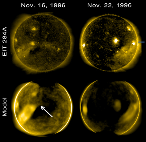
Figure 3. SOHO/EIT images vs. synthesized images in the 284 Å band. The top row shows the observations while the bottom row shows the images synthesized from AWSoM. The left column shows images for 1996 November 16 (i.e., a week prior to the observation time), and the white arrow points to the approximate location of the intersection between the SUMER slit and the plane of the sky. The right column shows the images for 1996 November 22. The approximate location of the SUMER slit is superimposed on the observed image.
Download figure:
Standard image High-resolution image6.2. Comparison of Synthetic and SUMER Spectra
In order to perform 3D line-of-sight analysis, we begin by extracting model results, such as the electron and proton densities, and temperatures, as well as the Alfvén wave energy density, along the line of sight to the SUMER observational slit. The geometry of the problem is illustrated in Figure 4, where the SUMER line of sight for the entire slit width is traced within the three-dimensional space of the model solution. The figure shows the solar surface, colored by the radial magnetic field magnitude, the horizontal plane containing the SUMER slit colored by the electron density, and the plane of the sky for the time of SUMER observations.
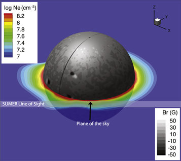
Figure 4. SUMER lines of sight in the 3D model domain. The spherical surface is the solar colored by the radial magnetic field. The ecliptic plane is colored by the electron density from the model. The SUMER line of sight lies in the same plane and is marked by the thick gray line. The black arrow marks the “plane of the sky,” i.e., the plane perpendicular to the line of sight and in which the SUMER slit passes closest to the solar surface.
Download figure:
Standard image High-resolution imageUsing the model results and the CHIANTI database, we calculated the spectral flux line-of-sight integral according to Equation (20) for each of the lines in Table 2 at each of the 30 radial sections of the SUMER slit. The resulting spectra are compared to the observed spectra in Figures 5–9. The left panel in each figure shows a contour plot of the synthetic and observed line spectra at all heights covered by the SUMER slit. The middle panel compares the line profile in absolute units at two different distances above the limb: 1.04 R⊙ and 1.14 R⊙. The blue symbols and error bars show the observed flux and the associated uncertainty, which takes into account a calibration error of 20% for SUMER detector B (Wilhelm 2006), and the statistical error in the photon count. The blue curve shows the fit to a Gaussian of the measured flux. The red curve shows the model result. On the right, we show the normalized line profile in each of these heights, using the same color coding as before. The normalized line profile allows us to examine the accuracy of the model prediction of the line width, independent of the absolute value of the predicted total flux. The first thing to notice is that for all lines, the observed and predicted line widths are in good agreement at both heights. These results imply that the combination of thermal and non-thermal motions predicted by the AWSoM model is accurate. The predicted and observed spectral line fluxes are in good agreement for the Mg ix and Na ix ions, while the model underpredicts their magnitude in the S x, Fe xii, and Ne viii ions. We discuss possible causes of these discrepancies in Section 6.3.
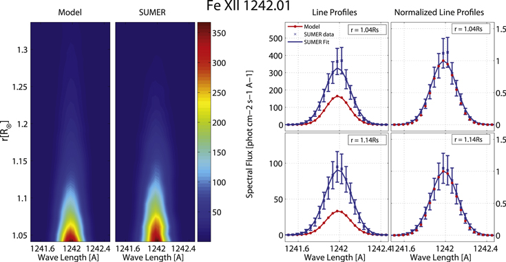
Figure 5. Comparison of synthetic and observed spectra for Fe xii 1242 Å. Left: color plots of the synthetic and observed spectra at distances  R⊙. Middle: selected line profiles extracted at r = 1.04 R⊙ (top) and at r = 1.14 R⊙ (bottom). Blue symbols with error bars show the SUMER data, the blue solid curve shows the fit to a Gaussian, and the red curve shows the line profile synthesized from the model. Right: normalized line profiles for the same heights. Curves are color-coded in the same way as the middle panels.
Download figure:
Standard image High-resolution image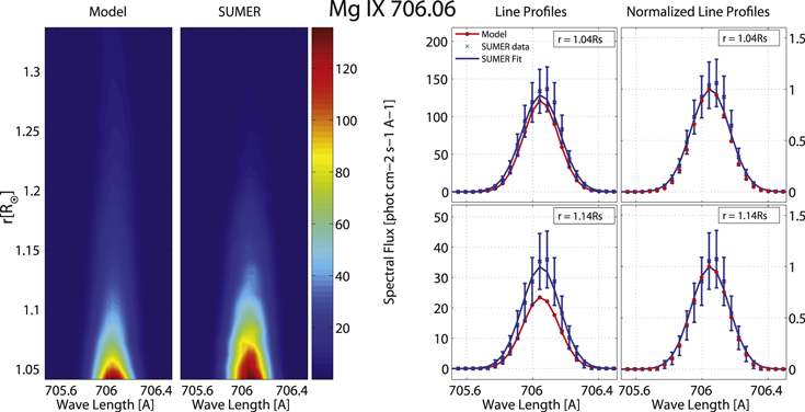
Figure 6. Comparison of synthetic and observed spectra for Mg ix 706 Å. See Figure 5 for the full description.
Download figure:
Standard image High-resolution image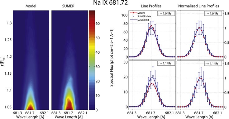
Figure 7. Comparison of synthetic and observed spectra for Na ix 681[A]. See Figure 5 for the full description.
Download figure:
Standard image High-resolution image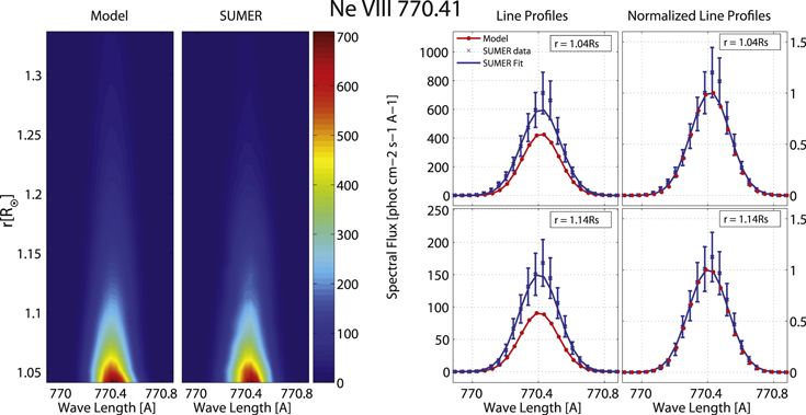
Figure 8. Comparison of synthetic and observed spectra for Ne viii 770 Å. See Figure 5 for the full description.
Download figure:
Standard image High-resolution image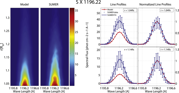
Figure 9. Comparison of synthetic and observed spectra for S x 1196 Å. See Figure 5 for the full description.
Download figure:
Standard image High-resolution image6.3. Comparison of Total Flux versus Height
The total flux predicted by the model depends on the distribution of electron density and temperature along the line of sight. In turn, the radial profiles of the electron density and temperature depend on the heating rate, which in our case is a result of turbulent dissipation of Alfvén waves. Thus, comparing the radial profiles of the total flux to the observations allows us to verify that the large-scale distribution of heating rates predicted by the model gives realistic results.
Figure 10 shows a comparison of the radial profiles of the total flux for all of the lines listed in Table 2. The left panels display the predicted and observed total flux, Ftot, at all heights covered by the SUMER slit. The panels on the right side of Figure 10 display the ratio between the observed and predicted total line fluxes as a measure to determine the agreement or disagreement between model and observations. The discrepancies between the model and the observations seem to decrease with radial distance, as all ions show agreement above 1.2 solar radii. However, this decrease is due in part to the increase with height of the uncertainties of the observed fluxes. The regions shaded by an orange color correspond to the height where the error in the measured flux is larger than the measured value itself. For these cases, the ratio between predicted and observed total flux becomes meaningless, and these points are excluded from the ratio calculation. The regions shaded in blue correspond to the height above the limb where the scattered light contribution may reach up to 50% of the observed line flux, as discussed in Section 4.2. These heights are summarized in the third column of Table 2. We next discuss the results for the separate lines in more detail.
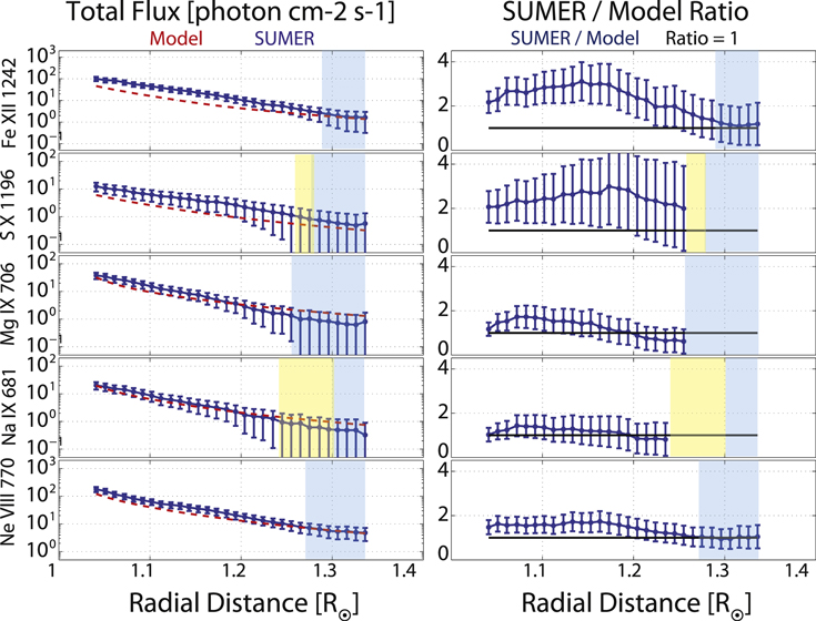
Figure 10. Total flux comparison. Left column: observed (blue) and predicted (red) total fluxes. Right column: ratio of observed to modeled total fluxes (blue curve). The black curve shows a ratio of 1, for convenience. The regions shaded in yellow correspond to heights where the uncertainty in the observed flux becomes larger than the measured value. In this case, the uncertainty in the ratio leads to a lower bound that is negative, and therefore, meaningless. The regions shaded in blue corresponds to heights above which the scattered light contribution might reach up to 50% of the observed flux, as reported in Table 2.
Download figure:
Standard image High-resolution imageMg ix and Na ix—The successful comparison for Mg ix and Na ix is very important. Since no atomic physics problems were expected for these lines (see Section 5.2), the agreement indicates that the overall temperature and density distributions predicted by the AWSoM model along the line of sight are realistic, although line-of-sight effects might compensate for local inaccuracies.
Fe xii—The total flux of the Fe xii line is underestimated, but it is important to note that the factor of 2 to 3 discrepancy we find is similar to the underestimation we expected from this line (see Section 5.2) so that the disagreement could be largely due to atomic data inaccuracies.
Ne viii and S x—The synthetic fluxes for Ne viii and S x are underestimated by a factor of ≈1.5 and ≈2, respectively. The S x line is density sensitive, and its contribution function  , defined by Equation (15), decreases as the electron density increases beyond
  cm−3: the underestimation might be stemming from an overestimation of the AWSoM-predicted electron density along the line of sight. However, no such effect is expected for Ne viii; thus, the underestimation of the flux must stem from a different reason and is most likely due to the uncertainties in the abundances of these two elements. In fact, the coronal abundances of S and Ne are uncertain, as they are affected by the still not-understood fractionation processes known as the “FIP effect” (Feldman & Laming 2000 and references therein). This effect consists in an enhancement of the coronal abundance ratio of elements with low (<10 eV) First Ionization Potential (FIP) to those with high (>10 eV) FIP over their photospheric values. Ne is a very high-FIP element (FIP = 21.6 eV) while S (FIP = 10.4 eV) sits at the threshold between the two classes of elements. The FIP bias of S is ill-determined: for example, the bias reported in Feldman et al. (1992), used in the present work, set it at 1.15, while Feldman et al. (1998) found a value between 1.2 and 2.0, which would solve this discrepancy. Furthermore, models of the FIP effect predict that S behaves as a high-FIP element in closed field lines in the corona, but exhibits enhancement in coronal holes and the fast solar wind (Laming 2015). The abundance of neon is even more uncertain as its absolute value cannot be measured in the photosphere and is usually inferred through the Ne/O abundance ratio. In turn, the coronal value of the Ne/O ratio itself is disputed: it is usually assumed to be 0.17 (Young 2005) but measurements carried out in the solar wind and in coronal holes have found that the coronal Ne/O is 0.1 (von Steiger et al. 2000; Landi & Testa 2015), is dependent on the solar cycle (Shearer et al. 2014; Landi & Testa 2015), and is much smaller than in the photosphere (Drake & Testa 2005). An additional complication comes from the fact that the value of the oxygen abundance in the photosphere and the corona is disputed as well. Thus, while we note that the coronal hole measurements of Landi & Testa (2015) would decrease the predicted intensities further and deepen the disagreement, we feel that the uncertainties in the neon coronal abundance are sufficiently large to account for the discrepancy until better determinations of that value are provided.
6.4. Comparison of Line Width versus Height
The comparison of the radial variation of the line width in the synthetic spectra to that found in the observations allows us to determine how well the predicted plasma and wave properties are able to account for the observed line broadening in the inner (1.04–1.34 R⊙) part of the equatorial solar atmosphere.
Figure 11 compares the radial profiles of the synthetic and observed line widths for each of the spectral lines in Table 2. The regions where the scattered light flux may contribute up to 50% to the line flux are shaded in blue. These radial distances are reported in Table 2. The panels on the left-hand side show the model and observed width cast in units of speed using Width (km s−1) =  , where c is the speed of light in km s−1. This quantity is often referred to as the effective speed. The blue curve with error bars shows the observations, while the red dashed line shows the model results. In order to examine the relative contribution from the thermal and non-thermal speeds, we repeated the calculation of the line widths while ignoring the non-thermal speed as a line-broadening mechanism. The results are shown as the green curves on the left panels. The panels on the right-hand side show the ratio of the observed to synthetic line width (blue curve). The solid black line denotes a ratio of 1, i.e., a perfect agreement. The first thing we note is that the ratios for all lines are all very close to unity, with a discrepancy of less than 10% at most heights. This implies that the combination of ion temperatures and non-thermal speeds predicted by AWSoM can produce synthetic line widths whose magnitudes are very close to the observed ones, at least in the case of the lower equatorial corona. As in the case of the total flux comparisons, we note that line-of-sight effects may compensate for any local inaccuracy in the AWSoM prediction. The removal of the non-thermal speed from the calculation of the synthetic profiles greatly reduces the agreement between the model and the observations. This implies that the non-thermal motions induced by the waves are necessary for predicting line widths that are consistent with observations. While the line width due to thermal motions alone does not change considerably with radial distance, the total line width which includes the wave-induced motions shows a clear radial dependence. This dependence is due in part to the effects of the magnetic topology, as we will discuss in Section 6.6. This comparison also sheds some light on the validity of our assumption that all the ions have the same temperature. The reasoning behind this assumption is that in the lower corona, where the density is still very high, collisions will allow the different ions to achieve thermal equilibrium. Since the spectral lines considered here are emitted by different elements, the thermal contribution to the line width is different for each of them, while the non-thermal contribution is the same. The simultaneous agreement of the predicted and observed widths for several ions make it less probable that their temperatures do in fact differ from one another. We note that the agreement between the synthetic and observed line widths decreases as the height above the limb increases for the case of Fe xii. This discrepancy may be due to the uncertainty in the observations, but it is also possible that our assumption that this ion, which has the largest mass of all of the ions considered here, also has the same temperature as the protons breaks down at higher altitudes, where the density has already fallen off considerably and the plasma becomes collisionless.
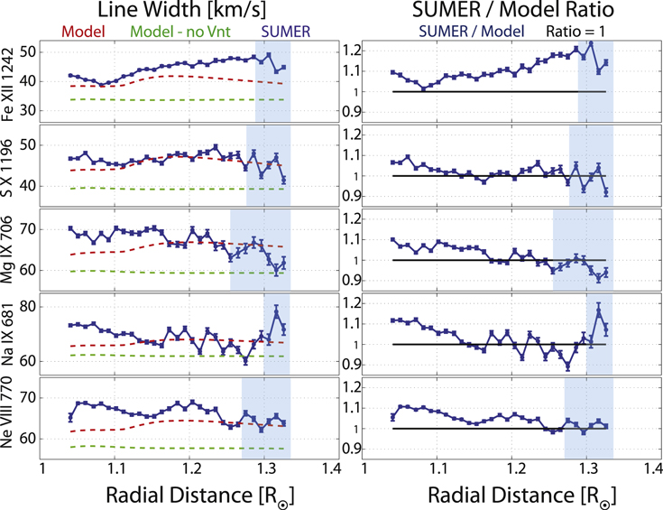
Figure 11. Model−SUMER FWHM comparison. Left column: observed (blue) and predicted (red) total fluxes. Green curves show the AWSoM prediction if the non-thermal speed contribution to the width is not taken into account. Right column: ratio of observed to modeled total fluxes (blue curve). The black line denotes a ratio of 1, for convenience. The regions shaded in blue correspond to heights above which the stray light contribution might reach up to 50% of the observed flux, as reported in Table 2.
Download figure:
Standard image High-resolution image6.5. Comparison of Electron Properties
In the previous sections, we showed that the modeled wave amplitude is consistent with the observed line widths of several different ions, suggesting that the model correctly predicts the amount of wave energy propagating in the corona. To complete this discussion, we wish to verify that the observed coronal heating rate, which depends on the wave dissipation rate, is also reproduced. Since the heating rate impacts the electron density and temperature, comparing the modeled and measured electron properties along the SUMER slit serves as an independent check of the dissipation mechanism assumed in the model. Oran et al. (2013) found that the AWSoM model’s prediction of the electron properties in a polar coronal hole during solar minimum was in good agreement with measurements. The simple geometry of the coronal hole allowed the authors to compare the line-of-sight measurements to model results extracted along the coronal hole axis. However, in the present case of observations of the equatorial quiet corona, which exhibits a more complex magnetic topology, it becomes less clear which region along the line of sight should be compared to the measurements. We therefore adopt a more detailed approach, one that takes into account the variable emission from the different magnetic structures crossing the line of sight.
6.5.1. Overcoming Line-of-sight Effects: 3D Emission Analysis
The advantage of a three-dimensional model is that it enables us, when combined with the CHIANTI atomic database, to calculate the relative contribution of each emitting volume along the line of sight to the total observed emission using the calculations presented in Section 5. This allows us to assess the amount of contamination to a given coronal structure from emission in the background and foreground, as well as guide us in the interpretation of diagnostic results. We here concentrate on the electron density and temperature diagnostics using line flux ratios; the electron density along the SUMER slit was measured using the line flux ratio of S x 1196 Å and S x 1212 Å, while the electron temperature was measured using the line flux ratio of Mg ix 706 Å and Mg ix 749 Å. In order to ensure that the comparison between the model and the diagnostics is valid, we must verify that we are sampling the model at a location that produces significant emission in both of the spectral lines used in the line-ratio diagnostics. Otherwise, we are comparing a random point in the model to the diagnostics. To translate this requirement into practical terms, we calculate the total line-of-sight emission of both lines, and then divide the local emission by that number. We thus get a measure of which locations have the most significant relative contribution to the line of sight. Next, we must ensure that both regions (for each spectral line) more or less overlap. Finally, we verify that the relative contribution of each region to the total line flux is the same for both lines. In this way, the ratio of the line fluxes integrated over the selected region will be equal to the ratio of line fluxes integrated over the entire line of sight. Only in this case can the modeled quantity in this region be compared to the measured one. It is also preferable, but not necessary, that this region be responsible for a significant fraction of the total emission. The procedure is somewhat different in the case of electron density and temperature measurements, and we discuss these separately.
6.5.2. Region of Maximum Emission for Electron Density Measurements
The electron density along the SUMER slit was obtained from the line flux ratio of the S x 1196 Å and S x 1212 Å lines. Figure 12 shows the relative contribution of each location along the line of sight to the total emission, calculated using the AWSoM results and the CHIANTI database. The left and right panels correspond to 1196 and 1212 lines, respectively. In each of the panels, the horizontal axes correspond to the radial distance for the 30 bins along the slit. The vertical axes represent the distance from the plane of the sky, measured in units of solar radii and ranging from −1 to 1. The regions outside this range have no clear emission pattern and are omitted for clarity. The top row shows the fractional contribution to the total emission along each point along the lines of sight. The bottom panels show the cumulative contribution to the normalized line-of-sight integral of the emission for these lines. The color scale ranges from 0 to 1 (corresponding to the two edges of the line of sight, i.e., the normalized integral equals 1 at the far end of the line of sight). It can be seen from the top panels of both lines that the largest relative contribution comes from a narrow region around the plane of the sky. Below r = 1.15 R⊙, there is a significant contribution coming from an additional region behind the central region. We have found that ∼24% of the total emission of both lines comes from a region that is less than 0.2 R⊙ wide, marked by the black and purple curves. The black curves show the bounds of the 24% region for S x 1196 Å, while the purple curves show the same for S x 1212 Å . Since the two regions more or less overlap, the line flux ratio calculated by integrating the line fluxes only over this region will be equal to the line flux ratio when the integration is over the entire line of sight. Therefore, the density modeled in this region is suitable for comparison with the density measurement using the S x 1196/1212 line flux ratio. It should be emphasized that this comparison is consistent, even though most of the total emission comes from outside this region. This is due to the line-ratio diagnostics. If another diagnostic method is used, the analysis should be different. We also note that the region we highlighted does not account for most of the total line-of-sight emission, but its relative contribution per unit length is much higher than other regions, and it possesses the most distinct emission pattern along the line of sight, while the relative contribution from the other regions is much smaller and structureless.
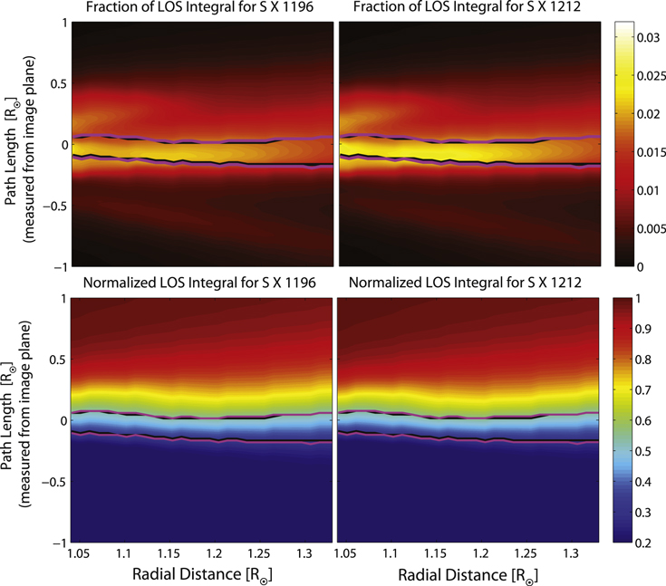
Figure 12. Relative contribution to the flux line-of-sight integral for S x 1196 Å (left column) and S x 1212 Å (right column) in the plane containing the SUMER slit. In all four panels, the horizontal axes show the radial distance for all 30 SUMER spatial bins, while the vertical axes show the distance from the plane of the sky. The top row shows the fraction of the total line-of-sight integral. The bottom row shows the cumulative contribution to the normalized line-of-sight integral. The purple curves represent the ranges along the line of sight that account for 24% of the total emission of S x 1196 Å, while the black curve represents the region that accounts for 24% of the total emission in the S x 1212 Å line.
Download figure:
Standard image High-resolution imageWe next locate this region in the model’s three-dimensional magnetic topology. Figure 13 shows the MHD solution in an equatorial plane. The color contours show the radial speed while the black curves show the magnetic field. (Both the velocity and magnetic field are readily simulated by the model, which is based on the MHD equations). The boundaries of the 24% region for S x 1196 Å are marked by the white squares (corresponding to the purple curves in Figure 12). Interestingly enough, we see that a large part of the emission is coming from a distinct magnetic structure of a pseudo-streamer, i.e., a loop structure topped by open field lines of a single polarity. The flow speed above the streamer is slower than that in the surrounding regions.
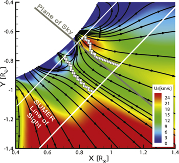
Figure 13. Location of maximum emission for S x 1196 Å. The color contours show the radial flow speed in the equatorial plane containing the SUMER lines of sight (marked by the two white lines). The gray line denotes the plane of the sky for the day of the observations. The black stream lines show the magnetic field. The white squares show the bounds of the line-of-sight segments corresponding to the purple curves in Figure 12.
Download figure:
Standard image High-resolution image6.5.3. Region of Maximum Emission for Electron Temperature Measurements
The electron temperature along the SUMER slit was obtained from the line flux ratio of Mg ix 706 Å and Mg ix 749 Å. As for the S x line pair, we wish to verify that both lines give a similar relative contribution to the line-of-sight emission in the same region. The cumulative contribution along the line of sight is shown in Figure 14. The overlaid curves represent the region where the relative contributions of the two lines are similar, and account for 36% of the total line-of-sight emission. The black and purple curves correspond to the 706 Å and the 749 Å lines, respectively. As can be seen, these regions almost entirely overlap. Calculating the temperature from the observed line flux ratio also requires us to know the electron density, which we take from the measurement discussed in the previous section. We therefore wish to compare the location of the region of equal contribution of the Mg ix lines to the region of equal contribution of the S x lines, i.e., the pseudo-streamer region selected in the previous section. The comparison is shown in Figure 15. The panels show the fractional contribution for Mg ix 749 Å (left) and for S x 1212 Å (right). The purple curves represent the region of equal contribution of the S x line pair (as in Figures 12 and 13), while the black curves represent the region of equal contribution of the Mg ix line pair (as in Figure 14). As can be seen, the spatial distributions of the emission are quite different, mostly at low altitudes. The regions of equal contribution more or less overlap above a heliocentric distance of 1.15 R⊙. We therefore restrict the comparison of the measured and predicted electron temperatures to these altitudes only, where we can safely assume that the density and temperature observations apply to the same region. Examining Figure 13, we can see that this altitude corresponds to the purely open field line region of the pseudo-streamer, while at lower altitudes the lines of sight intersect both open and closed field line structures.
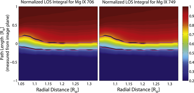
Figure 14. Cumulative contribution to the normalized line-of-sight integral of the Mg ix 706 Å (left) and Mg ix 749 Å (right) fluxes in the plane containing the SUMER slit. Horizontal axes show the radial distance for all 30 SUMER spatial bins, while vertical axes show the distance from the plane of the sky. The top row shows the fraction of the total line-of-sight integral. The purple curves represent the ranges along the line of sight that account for 36% of the total emission of the 706 Å line, while the black curves represent the same range for the 749 Å line.
Download figure:
Standard image High-resolution image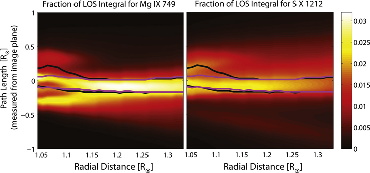
Figure 15. Comparison of the relative contribution of the Mg ix and S x line pairs along the SUMER line of sight. Color contours show the fractional contribution to the line-of-sight integral of the flux of Mg ix 749 Å (left) and S x 1212 Å (right). The purple curves represent the ranges along the line of sight where the S x line pair has similar contribution (same region as in Figure 12), while the black curves represent the region where the Mg ix line pair has a similar contribution (same region as in Figure 14).
Download figure:
Standard image High-resolution image6.5.4. Electron Density and Temperature in a Pseudo-streamer
We located a distinct and narrow region that accounts for equal parts of the total fluxes of the lines used in the electron density and temperature measurements. For each line of sight, we average the predicted quantity over the segment bounded by the white squares in Figure 13 to obtain a radial profile along the SUMER slit.
Figure 16 shows the comparison of the predicted electron density in the pseudo-streamer with the SUMER measurement. The blue curve with the error bars shows the measured electron density while the dashed red line shows the model results. The error bars in the measured density is a result of the error in the measurement of the line fluxes participating in the line-ratio calculation. The line flux errors were discussed in Section 6.2. The error bars in the model indicate the minimum and maximum electron densities found along the line-of-sight segments over which we take the average. The shaded region represents the altitude where the observed flux of the lines used for this measurement has decreased to below twice the scattered light flux, making the measurement less reliable at these heights. As can be seen, the modeled density falls inside the measured ranges at all altitudes, although the uncertainty in the electron density measurement is quite large.
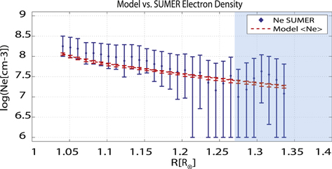
Figure 16. Model/SUMER electron density comparison. The blue curve shows the density measured using the SUMER S x 1196 Å and S x 1212 Å line flux ratio. The red curve shows the modeled density, averaged over the line-of-sight segments bounded by white squares in Figure 13. The model uncertainty is calculated given the minimum and maximum densities along each segment. The shaded region represents the altitude above which the scattered light contribution to the observed line fluxes can reach up to 50% (see Table 2).
Download figure:
Standard image High-resolution imageThe predicted electron temperature along the SUMER slit and its comparison to observations is shown in Figure 17. The color coding, as well as the role of the error bars, is the same as in Figure 16. The comparison starts at r = 1.15 R⊙ since below that height the lines used in the temperature measurement are not emitted from the same region as the lines used for the density measurement. The shaded region corresponds to the altitudes where the observed flux of the lines used for this measurement has decreased to below twice the scattered light flux, making the measurement less reliable at these heights. The measured temperature exhibits large uncertainties and variations with height, with no clear radial trend. The predicted electron temperature falls within the range of observed values, suggesting that the heating supplied by the heating mechanism is sufficient to achieve the observed coronal temperatures in the quiet corona.
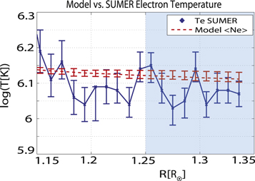
Figure 17. Model/SUMER electron temperature comparison. The blue curve shows the temperature measured using the SUMER Mg ix 706 Å and Mg ix 749 Å line flux ratio. The red curve shows the modeled electron temperature, averaged over the line-of-sight segments bounded by white squares in Figure 13. The model uncertainty is calculated given the minimum and maximum densities along each segment. The shaded region represents the altitude above which the scattered light contribution to the observed line fluxes can reach up to 50% (see Table 2).
Download figure:
Standard image High-resolution image6.6. Wave Dissipation in the Pseudo-streamer
The three-dimensional, magnetogram-driven solution allows us to study not only the synthetic line-of-sight line width, but also the variation of the wave amplitude along selected field lines. We recall that the line width observed from a particular direction depends on both the wave energy and the magnetic topology, as is clear from Equation (2). Examining Figure 13, we can see that the magnetic field in the region of largest emission is composed of a closed loop structure up to a radial distance of ∼1.1 R⊙, above which all field lines are open. In the closed loop region, the magnetic field direction changes from approximately perpendicular to parallel to the line of sight. Thus, while the wave amplitude is expected to increase with height in this region (due to the sharp decrease in the plasma density), its fraction that lies along the SUMER line of sight will decrease. Above the closed loop structure, the magnetic field direction is very close to perpendicular to the line of sight, and thus a larger share of the wave-induced motions will contribute to the line width. This dependence on the line of sight and magnetic field geometry is illustrated in the radial variation of the line widths in Figure 11, where an evident change in the synthetic line widths of all ions occurs around r = 1.1 R⊙.
In order to study the actual variation of the wave amplitude, we extracted the model results along three open field lines inside the region of largest emission. This will enable us to remove the effects of the line-of-sight geometry and directly study the wave dissipation taking place in this region. We calculate the rms of the wave velocity amplitude,  , using Equation (12). Hassler et al. (1990) and Moran (2001) have shown that if no wave damping is taking place, the rms wave amplitude would vary as
  as a result of energy conservation along a magnetic flux tube. Thus, we would expect the rms wave amplitude predicted by the model to be lower than the undamped values. The results are shown in Figure 18. The location of the selected field lines is shown in the inset. Line 1, colored in blue, is an open field line on the edge of the pseudo-streamer, while line 3, colored in red, is the first open field line straddling the closed loop structure. Line 2, colored in green, lies in between the other two lines. The solid curves show the wave amplitude as a function of the path length S along each of the field lines, while the dashed curves show the hypothetical curves for the wave amplitude assuming no dissipation, normalized to the value of the corresponding modeled curve at S = 0.05 R⊙. As expected, the rms wave amplitude sharply increases close to the inner boundary due to the sharp drop in density. Departures of the simulated wave amplitude from the curve of undissipated waves become prominent above
  R⊙, although each of the field lines exhibit a different dissipation rate. It is interesting to compare the curves for dissipated and undissipated waves to a similar analysis presented in Hahn et al. (2012) for a polar coronal hole. In Figure 5 therein, the observed effective speeds of several emission lines are compared to undamped values. Departures from the undamped wave amplitude curves start above heights of 0.1 R⊙ and 0.2 R⊙ above the limb, depending on the ion. Of the three field lines in Figure 18, line 1 most resembles a coronal hole field line, as it is an open line with minimal bending around the closed loop structure. The wave amplitude along line 1 shows very similar behavior to the one reported in Hahn et al. (2012). For line 2 and line 3, the wave amplitude of the dissipated waves shows larger departures from the non-dissipated case, with more wave energy being converted into heat. This is most prominent for line 3, where the wave amplitude is significantly reduced near the tip of the loop structure. In this location, higher dissipation is expected to occur due to the presence of counter-propagating waves, and the first term under the square root in Equation (10) will be taken into account. Above that point, the rms wave amplitude increases at a rate similar to that of line 1, consistent with the fact that the dissipation rate is now dominated by reflections, i.e., the second term under the square root in Equation (10). Line 2 also exhibits a signature of this behavior, although it is less pronounced.
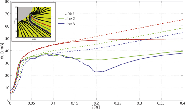
Figure 18. Model results of the rms velocity amplitude of the Alfén waves along three open field lines. In each color-coded pair, the solid curve shows the rms velocity amplitude extracted from the AWSoM model, while the dashed curve shows a hypothetical dependence for undamped waves for the same field line. The hypothetical curves were normalized to the corresponding modeled value at S = 0.05 R⊙. The inset shows the field lines in an equatorial plane (same as in Figure 13). White squares denote the region of maximum emission of the S x line pair as described in Section 6.5.1.
Download figure:
Standard image High-resolution image7. Conclusions
In this work, we have examined whether the dissipation of Alfvén waves due to a turbulent cascade is a viable mechanism to explain the observed large-scale distribution of coronal heating rates. By combining results from an Alfvén wave-driven MHD model with the CHIANTI atomic database, we were able to produce, for the first time, synthetic EUV spectra that include thermal and non-thermal broadening from a global model, and compare them to observations.
The ability to predict non-thermal line broadening in a wave-driven global model is an important step in testing the validity of the underlying wave-heating mechanism, as this observable is directly related to wave-induced motions and is a measure of the modeled amplitude of the Alfvén waves. The advantage of a global model is that the predicted emission is integrated over the line of sight using the full three-dimensional solution, without invoking simplifying assumptions about the geometry of the system.
Comparing the synthetic spectra to detailed SUMER observation between r = 1.03–1.43 R⊙, we tested whether the AWSoM model can predict plasma properties and wave energies that are simultaneously consistent with observations. The predicted total flux in the selected emission lines depends on the electron density and temperature, while the line width depends on the ion temperature and wave amplitude. We found good agreement between the predicted and observed line widths, and reasonable agreement of the total flux, given the uncertainties in atomic data.
By taking advantage of the three-dimensional nature of the solution, we could calculate the relative contribution of the different regions along the line of sight to the observed emission. We found that a substantial fraction of the emission of several lines comes from a narrow, well-defined magnetic structure: an equatorial pseudo-streamer. The electron density and temperature predicted by the model are in good agreement with the measurements performed using the emission of these lines, suggesting that this region is indeed the source of the relevant radiation detected by SUMER. This type of three-dimensional line-of-sight analysis is important to the interpretation of any remote observation.
There are several ways in which the results presented here can be improved. First, the synthetic profiles can be calculated more accurately. The line flux calculations used here were based on the assumption of ionization equilibrium. This assumption may break down, as wind-induced departures from equilibrium may occur. A more accurate calculation should be based on solving the charge state evolution in the region under question, which will be the basis of a more accurate calculation of the line fluxes (Oran et al. 2015, for example). However, this calculation will not change the simulated wave amplitudes, and thus, in general, will not bring about different line widths. Second, the model’s treatment of wave propagation and dissipation can be improved. Most notably, our treatment of wave reflections is not done self-consistently, as the reflection coefficient should depend on the magnetic topology. This requires a much more complex treatment of the wave field and its coupling to the MHD plasma, giving rise to a variable reflection coefficient (as in the coronal models in, e.g., Cranmer et al. 2009; van der Holst et al. 2014).
In summary, we have shown that the treatment of Alfvénic energy as described in the AWSoM model simultaneously produces electron densities, temperatures, total line fluxes, and line broadening that are consistent with observations. This suggests that the model describes the transport of wave energy as it travels from the top of the chromosphere into the corona, and the rate at which this energy is converted to heat, in a way that is consistent with observations of both the plasma temperatures and the wave amplitudes. This should be taken together with the fact that the same model, with the same heating mechanism, also produces solar wind speeds and heavy ion compositions that are consistent with Ulysses observations (Oran et al. 2015). This suggests that turbulent dissipation of Alfvénic perturbations is indeed a viable mechanism for driving coronal heating. Further work can shed light on how predictions tested in this work would compare to predictions made with other dissipation mechanisms. However, this work implies that, by and large, Alfvénic perturbations are very likely drivers of coronal heating and wind acceleration, as they reproduce a variety of observables that are currently not matched by alternative theories, such as heating by nano-flares (see, e.g., Klimchuk & Bradshaw 2014).
This work was supported by the NSF grant AGS-1322543 (Strategic Capabilities). The work of E.L. is supported by NASA grants NNX10AQ58G, NNX11AC20G, and NNX13AG22G. The simulations performed in this work were made possible thanks to the NASA Advanced Supercomputing Division, which granted us access to the Pleiades Supercomputing cluster. The analysis of radiative processes was made possible through the use of the CHIANTI atomic database. CHIANTI is a collaborative project involving the following universities: Cambridge (UK), and George Mason and Michigan (USA).