The following article is Open access

A Practical Framework for Estimating the Repetition Likelihood of Fast Radio Bursts from Spectral Morphology

Wan-Peng Sun, Yong-Kun Zhang, Ji-Guo Zhang, Xiaohui Liu, Yichao Li, Fu-Wen Zhang, Wan-Ting Hou, Jing-Fei Zhang, and Xin Zhang

Published 2026 February 19 • © 2026. The Author(s). Published by the American Astronomical Society.
The Astrophysical Journal, Volume 998, Number 2Citation Wan-Peng Sun et al 2026 ApJ 998 339DOI 10.3847/1538-4357/ae3c85

PDF Opens in a new tab.

ePub

You need an eReader or compatible software to experience the benefits of the ePub3 file format.

Article metrics

596 Total downloads
0 Video abstract views

Dates

Received 2025 October 30
Revised 2026 January 4
Accepted 2026 January 20
Published 2026 February 19

Unified Astronomy Thesaurus concepts

Radio transient sources; Radio bursts; Classification systems

Journal RSS

Create or edit your corridor alerts

What are corridors?

Abstract

The repeating behavior of fast radio bursts (FRBs) is regarded as a key clue to understanding their physical origin, yet reliably distinguishing repeaters from apparent nonrepeaters with current observations remains challenging. Here we propose a physically interpretable and practically quantifiable classification framework based on spectral morphology. Using dimensionality reduction, clustering, and feature-importance analysis, we identify the spectral running r and spectral index γ as the most critical parameters for distinguishing repeaters from apparent nonrepeaters in the CHIME/FRB sample. In the γ–r space, repeaters preferentially occupy regions with steeper, narrower-band spectra, whereas nonrepeaters cluster in flatter, broader-band regions, resulting in a clear density separation. We further construct a probability map in the γ–r space based on Gaussian mixture model posterior analysis, revealing a clear gradient of repetition likelihood from ∼67% in the high-repetition region to ∼7% in the low-repetition region. This model also identifies several apparent nonrepeaters with high inferred repetition probability, highlighting them as priority targets for future monitoring. This framework provides a simple and generalizable tool for assessing repeatability in the CHIME/FRB sample and highlights the diagnostic power of spectral morphology in unveiling FRB origins.

Export citation and abstractBibTeX RIS

Previous article in issue

Next article in issue

Original content from this work may be used under the terms of the Creative Commons Attribution 4.0 licence. Any further distribution of this work must maintain attribution to the author(s) and the title of the work, journal citation and DOI.

1. Introduction

Fast radio bursts (FRBs) are millisecond-duration radio transients of extraordinary luminosity originating from cosmological distances (D. R. Lorimer et al. 2007; D. Thornton et al. 2013; L. G. Spitler et al. 2014; B. Marcote et al. 2017; S. P. Tendulkar et al. 2017; E. Petroff et al. 2022; B. Zhang 2023, 2024). Current observations indicate that FRBs originate at least from compact objects, and the burst detected from the Galactic magnetar SGR 1935+2154 has confirmed magnetars as a plausible origin for at least a subset of FRBs (C. D. Bochenek et al. 2020; CHIME/FRB Collaboration et al. 2020). Although their physical origins remain elusive, FRBs have emerged as powerful tools for probing the cosmic content (J. P. Macquart et al. 2020; Z.-W. Zhao et al. 2020; J.-G. Zhang et al. 2023a, 2025a, 2025b). FRBs are commonly classified as repeaters, which produce multiple events, or apparent nonrepeaters with only a single detected event (L. G. Spitler et al. 2016; CHIME/FRB Collaboration et al. 2021, 2023). However, whether all FRBs will eventually repeat or share a common progenitor remains a central and unresolved question in FRB research (B. Zhang 2023).

Previous studies have revealed statistical differences between repeating and apparently nonrepeating FRBs across multiple observational properties. Repeaters typically exhibit longer pulse durations, narrower bandwidths (P. Kumar et al. 2021; Z. Pleunis et al. 2021; CHIME/FRB Collaboration et al. 2023), and a pronounced downward frequency drift (the “sad trombone”), whereas nonrepeaters tend to manifest as shorter, broadband bursts (CHIME/FRB Collaboration et al. 2021; X. H. Cui et al. 2021; Z. Pleunis et al. 2021; K. Zhang et al. 2022). These contrasts were once taken as evidence for fundamentally distinct physical origins of the two populations. However, as observational samples have grown, these distinctions have blurred, as many repeaters now exhibit broader bandwidths and shorter durations (CHIME/FRB Collaboration et al. 2023; D. Zhou et al. 2025a), which were previously considered typical of nonrepeaters. This trend has led to an increasing overlap between the two populations in feature space. Furthermore, after correcting for exposure time and sensitivity, CHIME/FRB Collaboration et al. (2023) reported no clear bimodality in burst-rate upper limits between repeaters and nonrepeaters, leaving open the possibility that all FRBs may eventually repeat. Further evidence points to intrinsic links between the two populations, particularly in their energy output, suggesting that repeaters and nonrepeaters may arise from statistically similar underlying populations. For instance, F. Kirsten et al. (2024) found that the high-energy bursts of the hyperactive repeater FRB 20201124A closely align with the energy distribution of the overall nonrepeater population, implying that apparently nonrepeating FRBs could simply be rare and exceptionally bright events from repeating sources. Similarly, O. S. Ould-Boukattine et al. (2026) reported a consistent trend at the high-energy end for both populations. In other words, despite differences in properties such as pulse width and bandwidth, their energy-release behaviors notably overlap (G. Q. Zhang et al. 2021; Y.-X. Huang et al. 2025). These findings challenge the notion that FRBs comprise two fundamentally distinct classes and highlight the difficulties in classifying them based on existing observational criteria. Nevertheless, refining their separation in parameter space and identifying potential repeater candidates remain crucial for advancing FRB studies.

In recent years, numerous studies have attempted to distinguish repeaters from apparent nonrepeaters using supervised (J. W. Luo et al. 2023; A. Sharma & V. M. Rajpaul 2024; B. Kharel et al. 2026) and unsupervised (B. H. Chen et al. 2022; X. Yang et al. 2023; J.-M. Zhu-Ge et al. 2023; C. R. García et al. 2024; L. Liu et al. 2025a; M. Madheshwaran et al. 2025; D.-C. Qiang et al. 2025; W.-P. Sun et al. 2025; A. J. B. Júnior et al. 2026) machine learning approaches. Generally, the supervised approaches face the primary challenge of avoiding erroneous training and selecting representative, well-labeled datasets for robust model development. Given current observational limitations, inappropriate training sets or biases can lead to misleading classifications, necessitating caution in their application.

The unsupervised methods are particularly valuable for leveraging multidimensional observational parameters for dimensionality reduction and clustering. However, feature selection is critical for unsupervised clustering, and current studies exhibit substantial variability in the choice of input feature parameters. Because models differ in their sensitivity to input parameters, current studies have produced inconsistent clustering results and identified varying sets of key distinguishing features, making it difficult to evaluate the reliability of any single analysis. In principle, if there truly exist key physical parameters that optimally distinguish repeaters from nonrepeaters, independent methodologies should converge upon comparable separation criteria. The fact that current studies instead highlight different key physical features reflects the limited robustness of these approaches.

Overall, existing machine learning methods often rely on high-dimensional inputs and complex models, limiting their physical interpretability and generalizability. Moreover, their outputs are typically confined to binary classifications without accompanying probabilistic assessments, thereby constraining their practical utility for prioritizing and guiding follow-up observations.

To address these challenges, we propose a physically interpretable and statistically robust framework that estimates the probability of an FRB exhibiting repeater-like properties, thereby providing a probabilistic metric to inform follow-up strategies. In this work, we perform a systematic analysis of multidimensional observational parameters using an extended CHIME/FRB sample (combining the first CHIME/FRB catalog, CHIME/FRB Collaboration et al. 2021, with newly reported repeaters from CHIME/FRB Collaboration et al. 2023). The structure of our paper is as follows. In Section 2, we introduce the extended CHIME/FRB sample and the methods used in this work. Section 3 presents the clustering results and the discussions. In Section 4, we summarize our work.

2. Data and Algorithm Parameters

2.1. Data Sample Selection

This study draws on FRB observations from two samples.

1.
The first CHIME/FRB catalog (hereafter Catalog 1) comprises FRBs observed between 2018 July 25 and 2019 July 1 (CHIME/FRB Collaboration et al. 2021).
2.
The CHIME/FRB Collaboration (2023) catalog (hereafter Catalog 2023) includes repeating FRBs detected from 2019 September 30 to 2021 May 1 (CHIME/FRB Collaboration et al. 2023).

All data were recorded within a 400–800 MHz frequency range. Each FRB may consist of one or more pulses that appear as isolated peaks in the dynamic spectrum, referred to as subbursts (K. Brown et al. 2024; S. Z. Sheikh et al. 2024). Since different subbursts may exhibit distinct spectral characteristics and parameter values, each subburst is treated as an independent event in our analysis.

We merge the FRB samples from Catalog 1 with the confirmed repeating FRBs from Catalog 2023. We exclude six nonrepeating FRBs that lack flux measurements, as well as one burst from FRB 20210224A (Sub_num = 0) due to its large uncertainty in r, potentially compromising the reliability of subsequent analysis. The final dataset consists of 706 FRBs, including 494 nonrepeaters and 212 repeaters from 43 distinct sources.

2.2. FRB Feature Parameters

In our previous work (W.-P. Sun et al. 2025), we selected seven key observational parameters to characterize the intrinsic emission properties and morphological characteristics of FRBs. These include the flux (S_ν), fluence (F_ν), subburst pulse width (Δt_WS), scattering time (Δt_ST), spectral index (γ), spectral running (r), and lowest frequency (ν_Low). Particularly, the spectral index γ and spectral running r well characterize the spectral morphology of a single burst via (CHIME/FRB Collaboration et al. 2021)

where S(ν) is the flux at frequency ν, S₀ denotes the overall amplitude, and ν₀ = 400.2 MHz is a selected reference frequency. The spectral index γ controls the overall slope of the spectrum, while r introduces curvature by modulating the exponent logarithmically. These features are selected to capture the essential differences between repeating and nonrepeating FRBs in terms of their radiation mechanisms and propagation environments.

In the present study, we extend the feature set by incorporating two additional parameters related to spectral structure: the highest frequency (ν_High) and the peak frequency (ν_Peak). While ν_High was previously excluded to avoid potential biases introduced by truncation at CHIME’s upper frequency limit, we now reconsider such a parameter in light of accumulated data, aiming to more comprehensively characterize the spectral extent of FRBs within the 400–800 MHz band. Notably, the truncation itself may encode meaningful differences between the repeaters and nonrepeaters. The parameter ν_Peak is defined as the frequency at which each burst reaches its peak intensity within the observed band. Given the diversity in FRB spectral morphology, this parameter is expected to enhance the discriminative power of subsequent classification analyses.

Thus, we select a total of nine feature parameters in this study: S_ν, F_ν, Δt_WS, Δt_ST, γ, r, ν_Low, ν_High, and ν_Peak.

2.3. t-SNE Algorithm

In this study, we apply the t-distributed stochastic neighbor embedding (t-SNE; L. van der Maaten & G. Hinton 2008; L. van der Maaten 2014) algorithm to perform nonlinear dimensionality reduction on the multidimensional observational parameters of FRBs, enabling visualization of their similarity structure in a two-dimensional space. The t-SNE algorithm converts high-dimensional distances into conditional probability distributions to preserve local neighborhood relationships, making it well suited for revealing potential distribution patterns and cluster structures in high-dimensional data.

Table 1. Sensitivity of t-SNE Embeddings to the Choice of Perplexity, Evaluated Using Trustworthiness, Continuity, and Spearman Correlation

Perplexity	Trustworthiness	Continuity	Spearman Correlation
40	0.998	0.743	0.722
50	0.998	0.748	0.736
60	0.998	0.752	0.712
70	0.997	0.744	0.732
80	0.997	0.745	0.711

Note. Trustworthiness and continuity measure the preservation of local and global neighborhood structures in the low-dimensional embedding, while the Spearman correlation quantifies the consistency of pairwise distances between the original feature space and the embedding. The small variations across different perplexity values indicate the robustness of the t-SNE results, supporting the choice of perplexity = 60 for subsequent analyses.

Download table as: ASCII Typeset image

The quality of t-SNE embeddings depends primarily on three key hyperparameters: perplexity, early exaggeration, and learning rate. Among these, perplexity controls the trade-off between preserving local and global structure and is generally regarded as the most significant parameter. Early exaggeration enhances initial similarities to facilitate well-separated clusters, while the learning rate controls the step size in gradient descent, affecting the scale and separation of points in the low-dimensional embedding. A detailed description of these parameters can be found in the Scikit-learn documentation.⁸

In this work, the early exaggeration and learning rate are fixed to their commonly used values of 12 and 260, respectively, which are consistent with empirically recommended ranges and were found to yield stable embeddings in preliminary tests. To assess the robustness of the t-SNE embeddings, we vary the perplexity between 40 and 80 and evaluate stability using three quantitative metrics: trustworthiness, continuity, and Spearman correlation. The corresponding results are listed in Table 1. Trustworthiness measures the fraction of neighbors in the embedding that are also neighbors in the original high-dimensional space, while continuity quantifies the fraction of true neighbors that are preserved in the embedding (J. Venna & S. Kaski 2001). High values of both indicate good local structure preservation. The Spearman correlation further tests the monotonic relation between pairwise distances in the original and embedded spaces (S. Kokoska & D. Zwillinger 2000), providing a complementary global measure of fidelity. Across this range of perplexity values, all three metrics remain stable, indicating that the embeddings are robust. We therefore adopt a perplexity of 60 for the final results used in subsequent classification. It is worth noting that the t-SNE embedding coordinates themselves have no direct physical meaning; however, their relative positions encode the similarity relationships among FRBs in the original feature space.

3. Results and Discussion

3.1. t-SNE Results

Figure 1 presents the t-SNE embedding result for FRBs in both Catalog 1 and Catalog 2023. Red triangles denote repeaters, while blue squares represent apparent nonrepeaters. Overall, the FRBs exhibit a distinct bimodal clustering in the t-SNE embedding space, with most repeaters clustered in the lower right region and nonrepeaters predominantly in the upper left. Since t-SNE preserves local neighborhood relations, the observed separation likely reflects two dominant combinations of features, with certain regions of the parameter space (e.g., the lower right cluster) preferentially associated with repeaters. While the axes are not physically interpretable, this clustering pattern highlights a statistically significant association between FRB repetition behavior and their underlying properties.

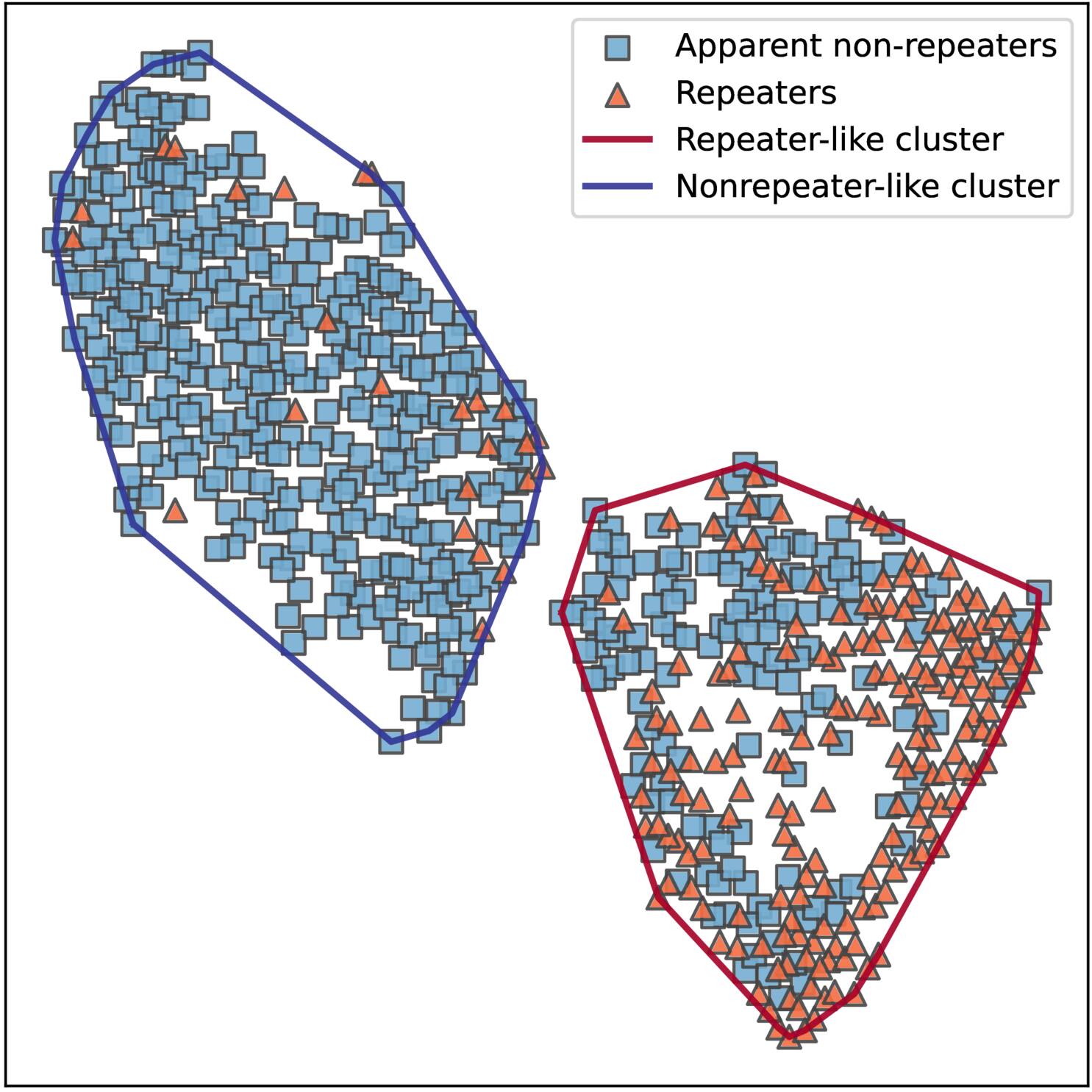
Figure 1. Refer to the following caption and surrounding text. — **Figure 1.** The embedding space of the t-SNE dimension reduction results and HDBSCAN clustering of FRBs in the CHIME/FRB Catalog 1 and Catalog 2023. Blue squares represent apparent nonrepeaters, while red triangles denote repeaters. The blue and red contours indicate the clusters identified by HDBSCAN, corresponding to the nonrepeater-like cluster and the repeater-like cluster, respectively.
Download figure:
Standard image High-resolution image

To further characterize the structure revealed by the t-SNE embedding, we apply the Hierarchical Density-Based Spatial Clustering of Applications with Noise (HDBSCAN; L. McInnes et al. 2017) algorithm for unsupervised, density-based clustering to extract statistically robust subgroups of FRBs. HDBSCAN is a density-based clustering method that does not require predefining the number of clusters and is well suited for identifying statistically significant groupings in complex, nonspherical structures, particularly within nonlinear embeddings such as those produced by t-SNE. As shown in Figure 1, HDBSCAN identifies two primary clusters, delineated by blue and red contour lines. To highlight their contrasting tendencies in repeating activity, we designate the cluster that includes the majority of repeating FRBs as the repeater-like cluster, emphasizing its strong statistical association with repeating FRB behavior. The cluster primarily composed of nonrepeating FRBs is referred to as the nonrepeater-like cluster, indicating a parameter configuration less likely to exhibit repeat activity.

While the repeater-like cluster is dominated by repeating FRBs, it also includes some apparent nonrepeaters. Conversely, the nonrepeater-like cluster consists primarily of apparent nonrepeaters but contains a few repeaters as well. Interestingly, some repeating bursts assigned to both clusters originate from the same repeating source. Those repeating bursts in the nonrepeater-like cluster are rare and tend to exhibit broader bandwidths, narrower pulse widths, and higher energies than typical repeater-like bursts, representing atypical repeating activity. Such cases demonstrate that repeaters can span a broad parameter space and occasionally resemble typical nonrepeaters, reinforcing the view that the two clusters reflect distinct but overlapping similarity patterns in the nine-dimensional parameter space, possibly shaped by different physical mechanisms or environments. Moreover, the distribution of repeaters within the repeater-like cluster itself appears inhomogeneous, suggesting the presence of substructures or subclusters that merit detailed investigation with larger samples in future studies.

Compared to our analysis of Catalog 1 in W.-P. Sun et al. (2025), we observe that clearly separating repeaters from nonrepeaters has become increasingly difficult, as reflected in the significant increase in the proportion of repeaters assigned to the nonrepeater-like cluster, from 0.3% to 4.9% in this study. These atypical repeaters account for approximately 12% of all repeaters. This rise indicates that parameter characteristics once thought exclusive to nonrepeaters can also appear in repeating sources, pointing to an increasingly continuous distribution of FRBs in feature space. This trend is corroborated by follow-up observations (CHIME/FRB Collaboration et al. 2023), which show that repeaters such as FRB 20181226F and FRB 20200127B exhibit broader bandwidths and narrower pulse widths, features previously associated with nonrepeaters. This finding implies that future investigations should explore the diversity and continuity in the parameter-space distribution of repeaters in more detail and examine the underlying physical processes or evolutionary scenarios that could account for the increasingly blurred observational boundary between repeating and nonrepeating FRBs.

3.2. Feature Importance

To further investigate the dominant roles of observational parameters in distinguishing the repeater-like and nonrepeater-like clusters, we construct a supervised classification model based on the CatBoostClassifier (L. Prokhorenkova et al. 2018), building on the HDBSCAN clustering results. We then apply the SHapley Additive exPlanations (SHAP; S. M. Lundberg & S.-I. Lee 2017) method to quantitatively interpret the contribution of each feature to the model output and identify the most influential parameters. SHAP is a game-theoretic model interpretation framework that estimates the marginal contribution of each feature to the model prediction, thereby revealing both the importance and directional influence of each feature.

Figure 2 presents the distribution of SHAP values for each feature parameter. The vertical axis lists the input features, sorted from top to bottom by their relative importance in influencing the model’s classification of FRBs into the two clusters. The horizontal axis shows the magnitude and direction of the SHAP values, reflecting each feature’s contribution and tendency toward classifying an event as belonging to either the nonrepeater-like or repeater-like cluster. The color gradient from blue to red indicates the variation in the corresponding feature values from low to high. It is important to note that, during model training, we define the repeater-like cluster as the positive class. Accordingly, a positive SHAP value implies that the corresponding feature value pushes the model toward classifying the sample as part of the repeater-like cluster, while a negative SHAP value indicates a tendency toward classification into the nonrepeater-like cluster.

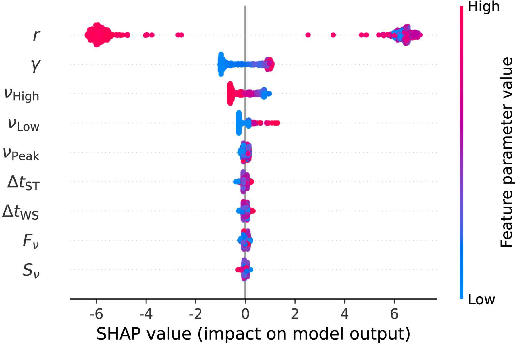
Figure 2. Refer to the following caption and surrounding text. — **Figure 2.** SHAP values for predictions in FRB classification. Features are ranked by overall importance, with the horizontal axis indicating the SHAP value, reflecting each feature’s impact on the model output.
Download figure:
Standard image High-resolution image

As shown in Figure 2, the spectral morphology parameters, i.e., r and γ, emerged as the top two most predictive features. These two features contribute significantly more than the others, consistent with our previous findings based on permutation feature-importance analysis (W.-P. Sun et al. 2025). This result indicates that the repeater-like and nonrepeater-like clusters exhibit pronounced differences in their spectral characteristics. Specifically, FRBs with lower (more negative) r values and larger γ values are more likely to be assigned to the repeater-like cluster. This is aligned with the physical picture in which repeating FRBs tend to exhibit narrower spectral morphologies (Z. Pleunis et al. 2021), potentially reflecting a preferred spectral morphology associated with their radiation mechanisms or propagation effects.

In addition, SHAP analysis highlights the significant contributions of the frequency-related parameters ν_High and ν_Low to cluster classification. Specifically, FRBs with higher ν_Low and lower ν_High, indicating a narrower bandwidth, tend to be classified into the repeater-like cluster. Conversely, FRBs with broader bandwidth (i.e., lower-frequency minima and higher-frequency maxima) are more likely to fall within the nonrepeater-like cluster. In contrast, temporal parameters (Δt_ST and Δt_WS) and intensity-related parameters (F_ν and S_ν) are assigned lower importance in the SHAP ranking. Nevertheless, Δt_ST and Δt_WS still exhibit modest directional trends: FRBs in the repeater-like cluster generally have broader pulse widths, whereas those in the nonrepeater-like cluster tend to show narrower widths. The spectral and temporal trends identified here through SHAP analysis are broadly consistent with previous findings, such as those by CHIME/FRB Collaboration et al. (2021, 2023), Z. Pleunis et al. (2021), and A. P. Curtin et al. (2025).

3.3. γ–r Parameter Distributions

3.3.1. γ–r Space Number Density Distribution

Based on the preceding SHAP analysis, this section focuses on the two most discriminative spectral parameters, γ and r, which effectively separate the repeater-like and nonrepeater-like clusters. According to the definition in Equation (1), the parameter r is closely related to the emission bandwidth and effectively characterizes the spectral turnover. This formulation captures a wide range of spectral morphologies: when r ∼ 0, the model reduces to a standard power law, indicative of broadband emission; in contrast, negative values of r correspond to spectra with a well-defined peak, characteristic of narrowband emission.

In this section, we aim to construct a simple observational framework using only r and γ to assess their ability to systematically differentiate repeaters from apparent nonrepeaters. Furthermore, we investigate their statistical correlations with the average burst rate, frequency bandwidth, and pulse width in order to gain deeper insights into the relationship between repeating behavior and observed diversity. Figure 3 illustrates the distribution of repeating (red) and apparently nonrepeating (blue) FRBs in γ–r parameter space.

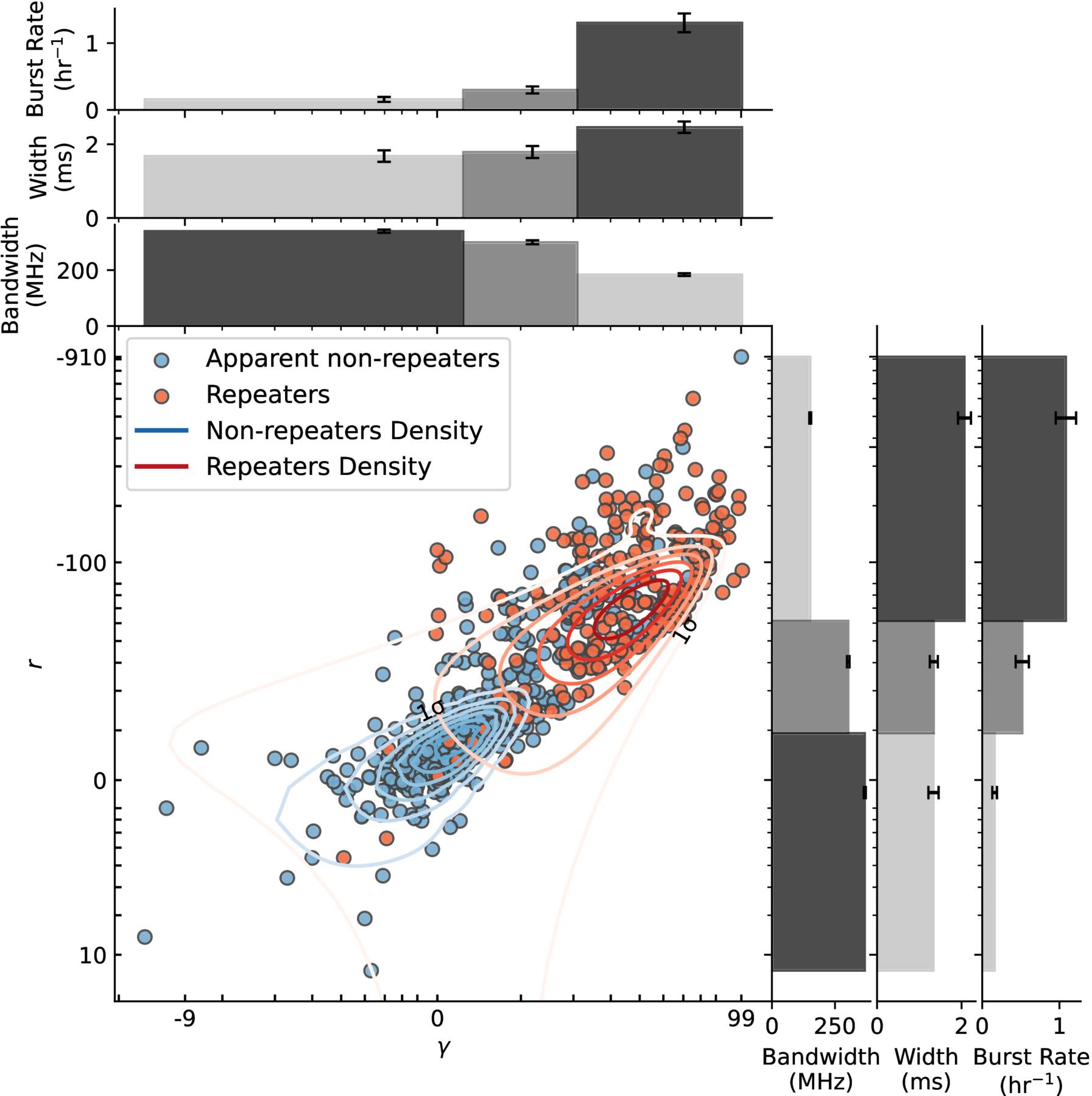
Figure 3. Refer to the following caption and surrounding text. — **Figure 3.** Distribution of repeaters (red) and apparent nonrepeaters (blue) in the γ–r parameter space, with red and blue contours overlaid to represent the density levels of each population. Marginal histograms show the distributions of bandwidth, pulse width, and burst rate, with error bars indicating the standard errors of the means.
Download figure:
Standard image High-resolution image

Although both repeaters and apparent nonrepeaters are present across the entire γ–r space, indicating overlap in their observed properties, they exhibit distinct preferences. The number density distributions of repeaters and apparent nonrepeaters are respectively fitted using the Gaussian mixture model (GMM⁹ ; F. Pedregosa et al. 2011). The best-fit results are shown as red and blue contours in Figure 3, where the outermost contour encloses 68% of the total sample. We observe distinct peak number densities for the two populations, indicating a systematic difference between repeaters and apparent nonrepeaters. Nevertheless, the 68% region of the repeaters substantially overlaps with the density peak of the apparent nonrepeaters. Specifically, most apparent nonrepeaters, located in the high number density region, exhibit small γ values and r ∼ 0, indicating relatively flat spectral profiles with minimal curvature, typically associated with broadband emission. In contrast, repeaters show a broader distribution, with their density peak shifted toward larger γ and more negative r values, and a low-density tail extending toward more extreme spectral shapes. This pattern suggests steeper spectra and narrower-band emission features.

To further evaluate the discriminative power of the two spectral parameters, r and γ, we calculate their combined classification performance. The resulting area under the receiver operating characteristic curve (AUC; T. Fawcett 2006) is 0.89, demonstrating strong separation between repeaters and nonrepeaters and confirming r and γ as reliable primary discriminators.

Overall, the γ–r space exhibits both continuity and multimodality. The significant separation between the density peaks of repeaters and nonrepeaters suggests that repetition correlates with specific spectral properties, potentially reflecting intrinsic differences in emission or propagation mechanisms. However, current evidence remains insufficient to conclusively determine whether repeaters and nonrepeaters originate from fundamentally distinct source classes. A more cautious interpretation is that the observed separation represents two characteristic regimes, possibly reflecting the extremes of a continuous spectrum of behaviors produced by a single population or physical process operating under different conditions, as discussed in Section 3.3.3.

3.3.2. γ–r Space Correlation with Bandwidth, Pulse Width, and Burst Rate

In the γ–r parameter space, we further examine the systematic variations of frequency bandwidth, pulse width, and FRB burst rate across different regions. Both bandwidth and pulse width have long been suggested to correlate statistically with repeating behavior (P. Scholz et al. 2016; CHIME/FRB Collaboration et al. 2019; 2021; 2023; E. Fonseca et al. 2020; Z. Pleunis et al. 2021; S.-Q. Zhong et al. 2022; Y. Zhu et al. 2024). Meanwhile, burst rate, defined as the number of detected bursts per unit time, represents an observational upper limit on the repeatability of an FRB over the observational timescale. The burst rate is estimated via

where N is the number of detected bursts, t_expo is the exposure time, F₀ = 5 Jy · ms is the adopted reference fluence threshold, and F_th denotes the observational fluence threshold for each FRB, provided by the CHIME/FRB collaboration. For the specific computation, we follow the method outlined by CHIME/FRB Collaboration et al. (2023), while for a more comprehensive statistical analysis, we include bursts detected during both the upper transit and lower transit. The exposure time is determined based on the precise sky position of each source (CHIME/FRB Collaboration et al. 2019). We reconsider the exposure time correction with both the transit status and the frequency-dependent beamwidth for each burst. To ensure uniform sensitivity across different sources, we adopt the fluence thresholds provided by the CHIME/FRB collaboration (CHIME/FRB Collaboration et al. 2021, 2023) using the method of A. Josephy et al. (2019), which accounts for variations of system gain, beam response, and bandwidth and applies the 95th percentile of the scaled threshold distribution per source. Finally, the burst rates for all sources are normalized to a fluence threshold of 5 Jy · ms, assuming a power-law energy distribution with an index of −1.5 (CHIME/FRB Collaboration et al. 2023).

In our analysis, we divide the sample into three equally populated bins along both the r and γ directions to ensure statistical robustness. Within each bin, we calculate the average frequency bandwidth, pulse width, and burst rate. The bar plots in Figure 3 visualize these statistics, with color gradients indicating the variation in average γ and r values. The results reveal a consistent trend: as one moves from the density peak of nonrepeaters toward that of repeaters in the γ–r parameter space, the frequency bandwidth gradually decreases, the pulse width increases, and the burst rate rises significantly. Our statistical analysis thus reveals both the positive correlation between repetition rate and pulse width and the negative correlation with bandwidth, consistent with the predictions of CHIME/FRB Collaboration et al. (2023) and supporting their proposed continuum framework that links burst morphology to repetition rate in a single repeating FRB population. This monotonic trend from the nonrepeaters to the repeater region further reinforces the link between spectral morphology and repeatability, supporting the scenario that spectral morphology serves as an important diagnostic for understanding the physical origin of FRBs.

3.3.3. Physical Interpretation within Geometric Frameworks

Based on the above analysis, FRBs in the γ–r space exhibit a positive correlation between repetition rate and pulse width and a negative correlation with bandwidth. These trends define a continuous, monotonic transition from nonrepeaters to repeaters, suggesting that the two populations may not arise from fundamentally distinct progenitor mechanisms. Instead, they more likely represent two manifestations of the same underlying mechanism or source class under different geometric and physical conditions, i.e., two extreme cases within a continuous distribution. The rotating polar cap scenario (P. Beniamini & P. Kumar 2025a; J.-W. Luo et al. 2025) provides a coherent framework for interpreting these results. In this framework, whether an FRB appears as repeating or nonrepeating, along with its associated spectral and temporal characteristics, is mainly governed by the viewing geometry of the line of sight relative to the magnetar’s emission cone. In the aligned-rotator geometry (α ≪ ρ), where α is the magnetic inclination angle and ρ is the half-opening angle of the emitting beam in the observer’s frame, the line of sight remains within a fixed emission region, so the physical conditions vary little, leading to pulse widths set mainly by the intrinsic burst timescale and spectra centered around a stable frequency. Such emission conditions can be naturally sustained in magnetars residing in binary systems (B. Zhang & R.-C. Hu 2025). This produces bursts with narrower spectra, longer widths, and higher repetition rates, corresponding to the clustering of repeating FRBs at r ≪ 0 and relatively large γ in Figure 3. In contrast, in the misaligned-rotator geometry (α ≫ ρ), the line of sight samples a wide range of surface regions as the beam sweeps by, causing large variations in emission conditions and yielding bursts with sweep-limited widths, broadened spectra, and lower apparent repetition rates. These correspond to the clustering of nonrepeating FRBs around r ∼ 0 and relatively smaller γ in the γ–r space. This geometric framework naturally explains the pronounced separation yet partial overlap of the density centers of repeating and nonrepeating FRBs observed in the γ–r plane (see Figure 3).

The geometry framework offers a potential explanation for the observed differences between repeating and apparently nonrepeating FRBs, although doing so hinges on restrictive geometric parameters. In particular, to simultaneously reproduce the nearly flat polarization position angles commonly observed in both repeating and apparently nonrepeating FRBs (D. Michilli et al. 2018; CHIME/FRB Collaboration et al. 2019; R. Luo et al. 2020; G. H. Hilmarsson et al. 2021a, 2021b; J.-C. Jiang et al. 2022; K. Nimmo et al. 2022; K. R. Sand et al. 2022; H. Xu et al. 2022a; P. Kumar et al. 2023; R. Mckinven et al. 2023; Y.-K. Zhang et al. 2023b; J. T. Faber et al. 2024; A. Pandhi et al. 2024; X. Liu et al. 2025b; C. Ng et al. 2025; J.-T. Xie et al. 2025), the rotating vector model (V. Radhakrishnan & D. J. Cooke 1969) requires that at least one of the following conditions be satisfied:

(1) an exceptionally long rotational period P ≫ Δt_WS,

(2) nearly aligned rotational and magnetic axes $\sin (\alpha )\sim 0$ , or

(3) a very small impact angle ∣β∣ ∼ 0.

For condition (1), the requirement of a long rotational period is expected for repeating FRBs, as current statistical analyses of large samples from some hyperactive repeating FRBs have excluded the existence of periods in the millisecond-to-second range (D. Li et al. 2021; J.-R. Niu et al. 2022; H. Xu et al. 2022a; Y.-K. Zhang et al. 2023b; P. Wang et al. 2025; J.-S. Zhang et al. 2025; D. Zhou et al. 2025b). In contrast, such a long period is not anticipated for nonrepeating FRBs, since their pulse width Δt_WS relies on the rotational cutoff. For condition (2), near alignment between the spin and magnetic axes is also plausible for repeating FRBs. However, for nonrepeating FRBs, this condition further requires α ≫ ρ. Under this premise, both α and ρ must be very small, which constitutes a highly restrictive constraint. For condition (3), the requirement of a very small impact angle applies equally to both types of FRBs. Beyond the geometric conditions discussed above, an alternative explanation for the observed disparities between the repeating and nonrepeating FRBs may lie in intrinsic variations within the emission mechanism itself, which also governs the resulting spectral morphology.

In addition, the power-law model for the frequency drift rate proposed by B. D. Metzger et al. (2022) naturally aligns with this geometric interpretation and provides a physical basis for the distribution differences between repeating and nonrepeating FRBs observed in Figure 3. This model characterizes the time–frequency evolution of FRBs by describing the drift rate of the central emission frequency using a power-law index $\bar{\beta }$ , such that ${\nu }_{c}(t)\propto {t}^{-\bar{\beta }}$ : smaller values of $\bar{\beta }$ correspond to more gradual frequency drifts, resulting in narrower spectra and longer widths, whereas larger $\bar{\beta }$ values lead to rapid frequency drifts, producing broader spectra and shorter widths. Combining this with our results, the parameters r and γ can be understood as observational descriptors of such time–frequency evolution: repeating FRBs cluster in the region with r ≪ 0 and relatively large γ, consistent with the small- $\bar{\beta }$ scenario, whereas nonrepeating FRBs are more distributed around r ∼ 0 with smaller γ, corresponding to larger $\bar{\beta }$ .

We note that in Figure 3, a small subset of repeaters falls within the primary density peak of apparent nonrepeaters. These bursts exhibit broader spectra and shorter durations and generally originate from only a few sporadic events of a given repeater. Their properties differ markedly from those of the majority of typical repeating bursts. This suggests that the emission region or emission mechanism of repeaters may not always remain stable and consistent. Instead, different physical processes, such as changes in the emission site or beaming angle, may occasionally produce short-duration, broadband, and potentially high-energy bursts that resemble those of apparently nonrepeating sources (F. Kirsten et al. 2024). In addition, such “outlier” events may also be explained by low-probability processes external to the emission source. For example, propagation effects such as plasma lensing can, on rare occasions, significantly modify the observed spectra of bursts (J. M. Cordes et al. 2017; E. Sobacchi et al. 2021; P. Kumar et al. 2024). However, their occurrence rate is expected to be extremely low, and thus they can only account for a small number of anomalous events. On the other hand, statistical fluctuations in a limited sample can naturally produce a few events located at the tails of the underlying parameter distribution, making these outliers statistically plausible. Consequently, the continuous distribution and density structure differences observed in the γ–r space may not only arise from geometric effects within a single theoretical framework but also reflect continuous manifestations of the same class of sources in different physical states (P. Beniamini & P. Kumar 2025b). This provides important observational clues for probing the origins and emission mechanisms of FRBs.

3.4. γ–r Framework for Repetition Probability Estimation

In this section, we construct an empirical probability map in the γ–r space to estimate the likelihood of FRBs exhibiting repeating behavior. In Figure 4, we draw dashed lines at the median values of r and γ for the entire FRBs, dividing the parameter space into four quadrants. This division approximately corresponds to the natural boundary between the density peaks of nonrepeaters and repeaters shown in Figure 3, reflecting that certain spectral morphologies are more likely to produce repeating FRBs.

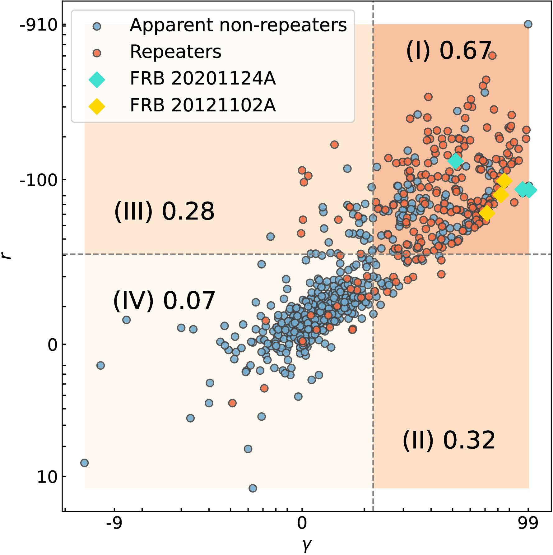
Figure 4. Refer to the following caption and surrounding text. — **Figure 4.** Distribution of repeaters (red) and apparent nonrepeaters (blue) in the γ–r parameter space. The background shading indicates regions of different inferred repetition probabilities, with annotated values representing the mean posterior probabilities derived from the Bayesian GMM analysis. FRB 20201124A and FRB 20121102A are highlighted as cyan and yellow diamonds, respectively.
Download figure:
Standard image High-resolution image

To further quantify this distinction, we incorporated a Bayesian posterior probability assessment based on GMM fitting to model the probability density of repeaters and nonrepeaters in the γ–r parameter space, thereby estimating the posterior probability that each FRB belongs to the repeater population. In this framework, the posterior probability for a given FRB point x = (γ, r) to be classified as a repeater is computed using Bayes’s theorem,

where p(x∣R) and p(x∣N) denote the class likelihood estimated by fitting the GMM separately to the repeater and apparent nonrepeater number density distribution (as shown with the contours in Figure 3), and π_R and π_N represent the corresponding prior probabilities, taken as the observed fractions of repeaters and nonrepeaters,

This formulation enables a probabilistic classification in which each FRB is assigned a continuous posterior probability of belonging to the repeater population, rather than a hard binary label.

Based on these posterior probabilities, we computed the average repetition probability within each region defined in Figure 4, obtaining values of 0.67 (I), 0.32 (II), 0.28 (III), and 0.07 (IV). This pronounced gradient demonstrates a clear dependence of FRB repeatability on the γ–r parameter space. In particular, the stark contrast between the high-repetition region I and the nearly nonrepeating region IV further quantifies the association between spectral morphology and repeat behavior. This result is consistent with the previous analysis based on density contours, reinforcing spectral morphology as a potential indicator for distinguishing repeaters.

Additionally, in Figure 4, we highlight two well-studied and highly active repeating FRB sources: FRB 20121102A and FRB 20201124A. Both have been monitored extensively with high sensitivity by the Arecibo telescope (J. N. Jahns et al. 2023) and FAST (D. Li et al. 2021; H. Xu et al. 2022b), yielding records of thousands of bursts, thereby providing critical insights into the origins of FRBs. Notably, both sources fall within the high-repetition-probability region I defined in our framework, serving as compelling evidence for the robustness and predictive usefulness of this spectral partitioning. Except for a small number of atypical repeating bursts, this framework successfully assigns approximately 80% of known repeaters to the high-probability region I. Overall, this probability map directly links FRB repeatability to spectral morphology parameters, offering a simple, physically interpretable prediction framework independent of prior labeling.

To assess the performance of the γ–r framework in assigning repetition probability scores, we randomly withhold 10% of known repeaters (corresponding to 21 FRBs) and 10% of apparently nonrepeating FRBs (49 FRBs) from the construction of the γ–r framework and build the framework using the remaining FRB sample. We then estimate the repetition probability scores for the held-out known repeaters.

Given the limited number of confirmed repeating FRBs in the current dataset, we repeat this procedure 100 times to evaluate the robustness of the framework under different random realizations. Figure 5 shows the distributions of the mean (left) and median (right) repetition probability scores for the held-out repeaters across 100 random subsampling realizations. While variations in the randomly selected subsets introduce modest fluctuations in the inferred scores, the mean repetition probability score averaged over all realizations is 0.65, generally consistent with the repetition probability density of region I in the full γ–r framework (Figure 4).

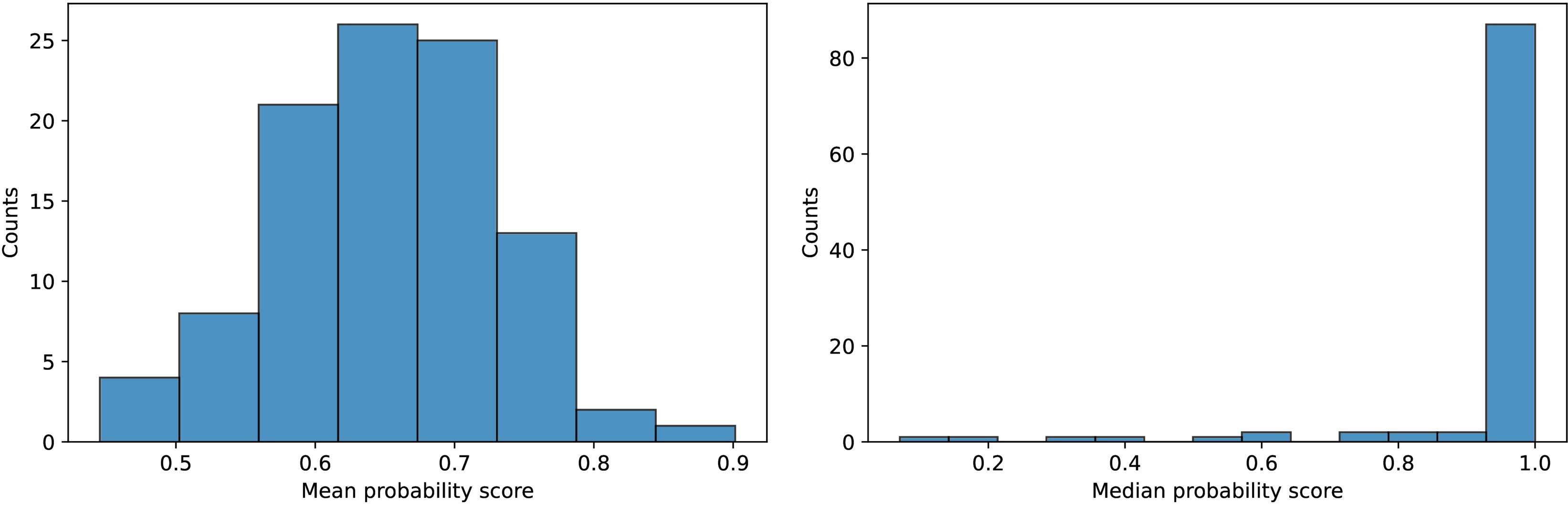
Figure 5. Refer to the following caption and surrounding text. — **Figure 5.** The left and right panels show the distributions of the mean and median repetition probability scores, respectively, for the randomly held-out 10% known repeaters, obtained from 100 random subsampling realizations, with repetition probability scores estimated using the γ–r framework.
Download figure:
Standard image High-resolution image

The median scores, which characterize the typical repetition probability of the held-out repeaters and are insensitive to a small number of extreme values, are strongly concentrated in the range 0.9–1.0 for the vast majority of realizations, with only a few cases extending into the intermediate-probability regime, consistent with the presence of a small number of repeaters with atypical spectral properties. This behavior indicates that, even when the framework is constructed from different data subsets, at least half of the held-out known repeaters are consistently assigned high repetition probabilities, demonstrating the robustness of the γ–r framework.

For future FRBs newly detected by CHIME, their positions in this map can be readily determined using only r and γ, enabling a preliminary estimation of their likelihood to exhibit repeating FRBs. This provides a practical and accessible tool for rapidly assessing repetition probability and prioritizing monitoring targets in future observations. Compared with machine learning classification methods that rely on multiparameter dimensionality reduction and clustering, this physically based partitioning is faster and more intuitive and yields robust, generalizable results.

We further combine the t-SNE results with the γ–r parameter map to identify a set of FRB sources that have not yet been observed to repeat but exhibit statistical characteristics closely resembling those of known repeaters. Specifically, we first selected all nonrepeating FRBs classified within the repeater-like cluster and categorized them according to their quadrant positions in the γ–r parameter space, with particular attention to those located in the high-repetition-probability region I.

We propose that these sources, which exhibit a high repetition tendency under multiple criteria, should be prioritized as high-probability candidates for follow-up monitoring with future telescopes. Appendix Table 2 lists the detailed information for these candidates, including their quadrant positions in the γ–r space, posterior probability scores derived from the GMM modeling, and corresponding r and γ values, providing a reference for future searches for repeaters and studies of spectral evolution.

4. Conclusion

In this work, we analyzed the repeatability characteristics of FRBs using an extended CHIME/FRB sample, integrating dimensionality reduction, clustering, feature-importance evaluation, and spectral-parameter-based partitioning. We further propose a simple and generalizable method that relies solely on spectral parameters to classify FRBs by their repeatability preference and effectively estimate their repetition probabilities. The main conclusions are as follows.

1.
Using t-SNE for dimensionality reduction and HDBSCAN for clustering, we performed unsupervised clustering on the combined CHIME Catalog 1 and Catalog 2023 samples, resulting in two clusters. One cluster, designated as the repeater-like cluster, exhibits a higher tendency to repeat and contains the majority of known repeaters, showing statistically significant differences from the other cluster, termed the nonrepeater-like cluster. SHAP-based feature-importance analysis confirms that the spectral running r and spectral index γ are the dominant parameters separating repeaters from apparent nonrepeaters, reinforcing the connection between spectral features and FRB repeatability. Consistently, we find that using r and γ alone yields an AUC of 0.89, demonstrating strong discriminative power and validating their role as primary distinguishing metrics.
2.
In the γ–r space, we find that the density centers of repeaters and nonrepeaters are clearly separated, though substantial overlap exists across the entire space. Furthermore, we identify a positive correlation between burst rate and pulse width and a negative correlation between burst rate and bandwidth in the γ–r space. These trends not only reinforce the physical link between spectral morphology and repeatability but also provide key insights supporting the possibility that FRBs belong to a single underlying population.
3.
The rotating polar cap scenario and the power-law model for frequency drift rates provide a coherent explanation for the distinct clustering of repeaters and nonrepeaters in the γ–r space, linking these distributions to geometric configurations and resulting variations in emission-region conditions.
4.
We construct a four-quadrant probability map in the γ–r space to rapidly assess the likelihood of repetition for different spectral parameter combinations. This map exhibits a pronounced statistical gradient, with repetition likelihoods of ∼67% in the high-repetition region and only ∼7% in the low-repetition region, demonstrating that the spectral morphology can serve as an effective predictor of repeatability tendencies. Notably, all three bursts from FRB 20201124A fall within the high-probability region I, validating the robustness of this framework. Thus, it provides a simple, quantifiable, and easily generalizable tool for predicting repetition probabilities, serving as a practical reference for future telescope observations and studies of FRB repeatability. In addition, we identify 40 apparent nonrepeaters with probability scores above 0.6 in region I and recommend them as priority targets for future monitoring (details in the Appendix).

In summary, this study reveals a significant statistical association between FRB repeatability and spectral parameters, demonstrating that repetition probabilities can be effectively predicted using only simple spectral-shape parameters. This approach establishes a paradigm for a label-independent, physically motivated probabilistic framework, providing practical guidance for the rapid identification of repeaters and the design of follow-up observation strategies.

Acknowledgments

We are very grateful to Alice P. Curtin, Ziggy Pleunis, and Mary Jiang for helpful discussions. We acknowledge the support of the National Natural Science Foundation of China (grant Nos. 12473001, 12533001, and 12575049), the National SKA Program of China (grant Nos. 2022SKA0110200, 2022SKA0110203), the China Manned Space Program (grant No. CMS-CSST-2025-A02), and the 111 Project (grant No. B16009). F.-W.Z. acknowledges the support from the National Natural Science Foundation of China (No. 12463008) and the Guangxi Natural Science Foundation (No. 2022GXNSFDA035083). Y.-K.Z. is supported by the Postdoctoral Fellowship Program and China Postdoctoral Science Foundation (grant No. BX20250158).

Data Availability

The list of apparent nonrepeaters identified in this work as high-repetition-potential candidates is provided in Table 2 in the Appendix and in a machine-readable format. All necessary data used in this analysis are included in this article and the Appendix.

Appendix

This work uses t-SNE embedding and clustering analysis based on multidimensional observational parameters, combined with the definition of high-repetition-probability regions in the γ–r parameter space, to identify a set of FRB sources that have not yet been observed as repeaters but lie significantly close to the known repeater distribution in feature space. Specifically, we selected all apparent nonrepeaters assigned to the repeater-like cluster, with special emphasis on those falling within the high-repetition-probability region I in the γ–r space, designating them as the highest-priority targets for future monitoring campaigns.

Table 2 provides detailed information for these candidate sources, including their R.A., decl., and dispersion measure (DM) and the nine feature parameters used in our analysis, i.e., S_ν, F_ν, Δt_WS, Δt_ST, γ, r, ν_Low, ν_High, and ν_Peak. Table 2 also indicates the assigned region for each FRB in the γ–r parameter space.

Table 2. High-repetition-potential FRB Candidates Identified from Apparent Nonrepeaters

Name	Sub_num	R.A. (J2000)	Decl. (J2000)	DM	S_ν	F_ν	Δt_WS	Δt_ST	γ	r	ν_Low	ν_High	ν_Peak	Quadrant	Probability Score
		(deg)	(deg)	(pc cm⁻³)	(Jy)	(Jy ms)	(ms)	(ms)			(MHz)	(MHz)	(MHz)
FRB 20190423B	0	$298.5{8}_{-0.210}^{+0.210}$	$26.1{9}_{-0.210}^{+0.210}$	584.949	0.87	7.00	2.490	3.000	62.40	−106.00	463.80	623.10	537.60	I	0.95
FRB 20181017B	0	$237.7{6}_{-0.230}^{+0.230}$	$78.5{0}_{-0.250}^{+0.250}$	307.369	1.06	6.50	2.310	4.300	61.00	−77.00	499.30	704.80	593.20	I	0.95
FRB 20190422A	1	$48.5{6}_{-0.200}^{+0.200}$	$35.1{5}_{-0.200}^{+0.200}$	452.302	0.60	9.10	2.310	2.700	54.20	−63.70	506.30	740.50	612.30	I	0.95
FRB 20190609A	1	$345.3{0}_{-0.280}^{+0.280}$	$87.9{4}_{-0.330}^{+0.330}$	316.643	3.60	10.40	2.120	0.500	55.00	−67.00	499.10	722.40	600.50	I	0.95
FRB 20190112A	0	$257.9{8}_{-0.015}^{+0.015}$	$61.2{0}_{-0.026}^{+0.026}$	425.847	1.40	16.20	1.640	11.010	57.10	−51.40	564.60	800.20	697.70	I	0.95
FRB 20180801A	0	$322.5{3}_{-0.059}^{+0.059}$	$72.7{2}_{-0.220}^{+0.220}$	655.728	1.11	7.90	0.580	5.540	60.00	−75.50	500.20	709.30	595.60	I	0.95
FRB 20190623B	0	$335.2{2}_{-0.180}^{+0.180}$	$46.1{2}_{-0.180}^{+0.180}$	1556.765	1.58	2.78	0.440	0.720	54.20	−57.10	526.20	786.40	643.30	I	0.95
FRB 20190609A	0	$345.3{0}_{-0.280}^{+0.280}$	$87.9{4}_{-0.330}^{+0.330}$	316.643	3.60	10.40	0.432	0.500	62.40	−84.00	491.00	683.40	579.30	I	0.95
FRB 20190428A	0	$170.7{3}_{-0.027}^{+0.027}$	$23.3{3}_{-0.150}^{+0.150}$	969.400	2.22	7.40	0.374	3.630	54.00	−48.80	560.10	800.20	696.00	I	0.95
FRB 20181129B	0	$307.5{6}_{-0.260}^{+0.260}$	$81.3{2}_{-0.340}^{+0.340}$	405.905	4.00	9.50	0.364	0.830	73.80	−112.00	482.30	642.70	556.80	I	0.95
FRB 20181231B	0	$128.7{7}_{-0.200}^{+0.200}$	$55.9{9}_{-0.180}^{+0.180}$	197.170	0.89	2.34	0.337	1.750	59.60	−60.00	540.60	800.00	657.70	I	0.95
FRB 20181228B	0	$250.4{3}_{-0.210}^{+0.210}$	$63.8{5}_{-0.210}^{+0.210}$	568.651	0.40	1.67	0.100	1.159	59.30	−353.00	401.50	471.80	435.20	I	0.95
FRB 20190423B	1	$298.5{8}_{-0.210}^{+0.210}$	$26.1{9}_{-0.210}^{+0.210}$	584.949	0.87	7.00	8.500	3.000	63.00	−116.00	455.60	604.10	524.60	I	0.90
FRB 20180916C	0	$107.1{5}_{-0.230}^{+0.230}$	$45.0{8}_{-0.240}^{+0.240}$	2252.873	0.39	2.10	4.060	5.100	47.00	−50.00	516.90	794.60	640.90	I	0.90
FRB 20190228A	0	$183.4{8}_{-0.005}^{+0.005}$	$22.9{0}_{-0.120}^{+0.120}$	419.083	1.79	35.80	2.250	18.910	52.60	−51.90	538.40	800.20	664.70	I	0.90
FRB 20190605D	0	$26.7{2}_{-0.230}^{+0.230}$	$28.6{2}_{-0.250}^{+0.250}$	1656.533	0.82	2.16	1.069	1.200	48.30	−50.80	520.40	796.60	643.90	I	0.90
FRB 20190329A	0	$65.5{4}_{-0.190}^{+0.190}$	$73.6{3}_{-0.270}^{+0.270}$	188.606	0.52	2.24	1.040	0.900	42.00	−272.00	400.20	473.90	432.30	I	0.90
FRB 20181213B	0	$183.5{2}_{-0.220}^{+0.220}$	$53.7{0}_{-0.230}^{+0.230}$	626.593	0.75	1.70	0.850	1.200	45.60	−45.10	529.60	800.20	664.00	I	0.90
FRB 20181221A	0	$230.5{8}_{-0.200}^{+0.200}$	$25.8{6}_{-0.210}^{+0.210}$	316.237	1.25	5.80	0.754	1.323	62.10	−128.00	446.10	583.30	510.10	I	0.90
FRB 20181203B	0	$47.3{1}_{-0.004}^{+0.004}$	$24.0{2}_{-0.120}^{+0.120}$	375.387	1.45	4.50	0.578	2.320	47.80	−43.60	550.80	800.20	693.20	I	0.90
FRB 20190519J	0	$296.2{1}_{-0.085}^{+0.085}$	$86.9{3}_{-0.300}^{+0.300}$	642.759	0.63	1.70	0.460	0.501	24.30	−259.00	400.20	461.00	419.50	I	0.90
FRB 20181117C	0	$53.2{1}_{-0.170}^{+0.170}$	$25.7{3}_{-0.180}^{+0.180}$	1773.739	1.57	3.00	0.100	2.370	48.60	−46.30	541.20	800.20	676.50	I	0.90
FRB 20190422A	0	$48.5{6}_{-0.200}^{+0.200}$	$35.1{5}_{-0.200}^{+0.200}$	452.302	0.60	9.10	3.220	2.700	42.00	−46.90	501.70	781.40	626.10	I	0.80
FRB 20190218B	0	$268.7{0}_{-0.220}^{+0.220}$	$17.9{3}_{-0.260}^{+0.260}$	547.868	0.57	5.90	2.050	14.100	46.20	−60.00	483.40	715.20	588.00	I	0.80
FRB 20190701C	0	$96.3{6}_{-0.230}^{+0.230}$	$81.6{3}_{-0.270}^{+0.270}$	974.195	0.88	2.50	1.440	1.800	46.20	−211.00	402.20	495.50	446.40	I	0.80
FRB 20190129A	0	$45.0{6}_{-0.210}^{+0.210}$	$21.4{2}_{-0.230}^{+0.230}$	484.761	0.49	5.00	1.130	10.200	43.00	−37.80	552.80	800.20	707.70	I	0.80
FRB 20190211A	0	$67.0{6}_{-0.190}^{+0.190}$	$68.6{4}_{-0.200}^{+0.200}$	1188.256	1.47	5.80	0.360	3.290	38.90	−39.30	515.00	800.20	656.00	I	0.80
FRB 20190101B	0	$307.7{7}_{-0.230}^{+0.230}$	$29.8{9}_{-0.230}^{+0.230}$	1323.906	1.02	4.40	0.320	5.160	41.70	−36.10	554.30	800.20	713.60	I	0.80
FRB 20190130B	0	$172.1{1}_{-0.160}^{+0.160}$	$16.0{5}_{-0.072}^{+0.072}$	989.031	0.77	2.95	0.265	0.769	55.40	−140.80	428.60	553.60	487.10	I	0.80
FRB 20190125A	0	$45.7{3}_{-0.240}^{+0.240}$	$27.8{1}_{-0.260}^{+0.260}$	564.701	0.37	2.60	3.210	4.100	36.00	−37.00	510.10	800.20	655.50	I	0.70
FRB 20180920B	0	$191.0{9}_{-0.230}^{+0.230}$	$63.5{2}_{-0.240}^{+0.240}$	463.400	0.35	1.70	2.330	1.730	12.30	−121.00	400.20	483.40	421.10	I	0.70
FRB 20181012B	0	$206.3{3}_{-0.210}^{+0.210}$	$64.1{5}_{-0.065}^{+0.065}$	715.189	0.49	1.44	0.560	0.260	20.90	−154.00	400.20	483.90	428.30	I	0.70
FRB 20181214A	0	$70.0{0}_{-0.180}^{+0.180}$	$43.0{7}_{-0.180}^{+0.180}$	468.148	0.16	0.41	0.533	0.442	23.30	−139.00	400.20	494.60	435.00	I	0.70
FRB 20190624B	0	$304.6{5}_{-0.068}^{+0.068}$	$73.6{1}_{-0.200}^{+0.200}$	213.922	16.50	20.00	0.372	0.400	34.80	−43.20	475.40	754.30	598.80	I	0.70
FRB 20180725A	0	$93.4{2}_{-0.039}^{+0.039}$	$67.0{7}_{-0.210}^{+0.210}$	715.809	1.70	4.10	0.296	1.100	38.20	−45.80	485.30	760.10	607.40	I	0.70
FRB 20190527A	0	$12.4{5}_{-0.200}^{+0.200}$	$7.9{9}_{-0.067}^{+0.067}$	584.580	0.47	10.10	2.670	5.080	47.00	−122.00	422.40	556.10	484.70	I	0.60
FRB 20190527A	1	$12.4{5}_{-0.200}^{+0.200}$	$7.9{9}_{-0.067}^{+0.067}$	584.580	0.47	10.10	2.470	5.080	30.70	−133.00	400.20	512.20	449.10	I	0.60
FRB 20190403E	0	$220.2{2}_{-0.086}^{+0.086}$	$86.5{4}_{-0.270}^{+0.270}$	226.198	3.90	76.00	2.200	18.200	31.70	−36.20	482.10	798.70	620.60	I	0.60
FRB 20181223B	0	$174.8{9}_{-0.220}^{+0.220}$	$21.5{9}_{-0.240}^{+0.240}$	565.655	0.68	4.10	1.570	3.500	33.30	−41.00	473.80	761.20	600.60	I	0.60
FRB 20190408A	0	$262.2{0}_{-0.230}^{+0.230}$	$71.6{0}_{-0.260}^{+0.260}$	863.380	0.64	1.51	0.839	1.000	35.70	−49.00	464.10	716.50	576.60	I	0.60
FRB 20190429B	0	$329.9{3}_{-0.240}^{+0.240}$	$3.9{6}_{-0.330}^{+0.330}$	295.650	0.74	5.00	6.380	7.800	99.00	−910.00	401.70	444.10	422.40	I	<0.60
FRB 20190128C	0	$69.8{0}_{-0.230}^{+0.230}$	$78.9{4}_{-0.380}^{+0.380}$	310.622	0.71	5.90	6.160	7.600	22.60	−55.00	400.60	603.20	491.60	I	<0.60
FRB 20181101A	0	$21.2{6}_{-0.011}^{+0.011}$	$53.8{8}_{-0.160}^{+0.160}$	1472.678	0.50	10.70	6.030	10.000	16.40	−37.70	400.20	636.80	497.40	I	<0.60
FRB 20181229B	0	$238.3{7}_{-0.230}^{+0.230}$	$19.7{8}_{-0.260}^{+0.260}$	389.047	0.42	4.90	3.360	5.100	22.00	−103.00	400.20	517.50	445.50	I	<0.60
FRB 20190409B	0	$126.6{5}_{-0.220}^{+0.220}$	$63.4{7}_{-0.210}^{+0.210}$	285.633	0.39	6.80	2.340	20.900	21.10	−34.10	420.60	707.30	545.50	I	<0.60
FRB 20181128C	0	$268.7{7}_{-0.023}^{+0.023}$	$49.7{1}_{-0.200}^{+0.200}$	618.350	0.39	3.40	2.300	2.320	27.40	−75.00	403.20	572.10	480.30	I	<0.60
FRB 20190422A	2	$48.5{6}_{-0.200}^{+0.200}$	$35.1{5}_{-0.200}^{+0.200}$	452.302	0.60	9.10	2.000	2.700	24.00	−32.00	444.80	763.70	582.80	I	<0.60
FRB 20181115A	0	$142.9{8}_{-0.039}^{+0.039}$	$56.4{0}_{-0.180}^{+0.180}$	981.613	0.44	1.92	1.830	2.100	19.60	−62.00	400.20	568.40	468.80	I	<0.60
FRB 20190403G	0	$81.7{4}_{-0.220}^{+0.220}$	$25.7{8}_{-0.250}^{+0.250}$	865.311	0.75	1.59	1.590	1.900	35.70	−76.00	425.50	603.20	506.60	I	<0.60
FRB 20190531C	0	$331.1{4}_{-0.240}^{+0.240}$	$43.0{0}_{-0.240}^{+0.240}$	478.202	0.37	1.20	1.450	1.900	18.30	−74.00	400.20	540.60	453.00	I	<0.60
FRB 20181218A	0	$5.0{6}_{-0.190}^{+0.190}$	$71.3{5}_{-0.076}^{+0.076}$	1874.406	0.83	1.59	1.390	0.221	19.00	−83.60	400.20	529.30	448.40	I	<0.60
FRB 20190519F	0	$165.6{3}_{-0.200}^{+0.200}$	$77.2{3}_{-0.220}^{+0.220}$	797.766	0.75	4.00	1.360	1.360	21.70	−86.40	400.20	534.40	453.90	I	<0.60
FRB 20180925B	0	$145.4{5}_{-0.210}^{+0.210}$	$20.9{9}_{-0.089}^{+0.089}$	667.866	0.76	2.70	1.150	1.400	15.00	−41.50	400.20	606.90	479.60	I	<0.60
FRB 20190629A	0	$6.3{4}_{-0.250}^{+0.250}$	$12.6{7}_{-0.260}^{+0.260}$	503.779	0.82	3.05	1.140	1.700	24.70	−35.30	440.10	733.60	568.20	I	<0.60
FRB 20190425B	0	$210.1{2}_{-0.100}^{+0.100}$	$88.6{0}_{-0.210}^{+0.210}$	1031.724	1.25	3.10	1.108	1.300	22.40	−65.60	400.20	572.60	474.80	I	<0.60
FRB 20190529A	0	$68.0{6}_{-0.220}^{+0.220}$	$40.3{2}_{-0.230}^{+0.230}$	704.450	0.47	1.45	1.040	1.500	24.20	−97.00	400.20	528.90	453.40	I	<0.60
FRB 20181221B	0	$306.3{1}_{-0.004}^{+0.004}$	$80.9{8}_{-0.028}^{+0.028}$	1395.021	0.97	3.30	1.037	1.100	25.30	−61.20	405.40	597.60	492.20	I	<0.60
FRB 20190530A	0	$68.7{4}_{-0.025}^{+0.025}$	$60.5{9}_{-0.200}^{+0.200}$	555.445	0.58	1.69	1.020	1.300	17.70	−91.00	400.20	517.30	441.10	I	<0.60
FRB 20190410A	0	$263.4{7}_{-0.230}^{+0.230}$	$-2.3{7}_{-0.380}^{+0.380}$	284.020	1.59	5.80	1.010	1.200	43.00	−85.00	437.40	607.90	515.70	I	<0.60
FRB 20190130A	0	$25.6{4}_{-0.240}^{+0.240}$	$13.1{6}_{-0.300}^{+0.300}$	1367.461	0.47	4.40	0.990	3.200	19.30	−62.00	400.20	567.20	467.70	I	<0.60
FRB 20190210E	0	$313.6{5}_{-0.280}^{+0.280}$	$86.6{7}_{-0.310}^{+0.310}$	580.580	0.69	1.45	0.960	1.100	13.40	−40.50	400.20	599.40	472.20	I	<0.60
FRB 20190304C	0	$223.0{1}_{-0.230}^{+0.230}$	$26.7{2}_{-0.250}^{+0.250}$	564.991	0.53	1.32	0.948	1.100	22.30	−87.00	400.20	535.20	454.90	I	<0.60
FRB 20190102A	0	$9.2{6}_{-0.180}^{+0.180}$	$26.7{2}_{-0.057}^{+0.057}$	699.173	1.12	4.20	0.824	0.986	28.90	−67.80	411.90	595.50	495.20	I	<0.60
FRB 20190206A	0	$244.8{5}_{-0.220}^{+0.220}$	$9.3{6}_{-0.260}^{+0.260}$	188.336	1.40	9.10	0.804	2.740	38.00	−65.70	443.20	644.60	534.50	I	<0.60
FRB 20181014C	0	$117.8{7}_{-0.220}^{+0.220}$	$41.5{9}_{-0.230}^{+0.230}$	752.167	0.57	1.48	0.790	1.000	18.00	−30.50	408.60	707.70	537.70	I	<0.60
FRB 20190223A	0	$64.7{2}_{-0.300}^{+0.300}$	$87.6{5}_{-0.320}^{+0.320}$	389.237	0.47	1.58	0.763	0.870	21.80	−103.00	400.20	516.50	444.80	I	<0.60
FRB 20181127A	0	$243.8{0}_{-0.230}^{+0.230}$	$25.4{3}_{-0.250}^{+0.250}$	930.317	0.78	2.90	0.740	0.582	18.50	−51.30	400.20	592.30	479.30	I	<0.60
FRB 20190625D	0	$115.0{2}_{-0.013}^{+0.013}$	$4.8{7}_{-0.033}^{+0.033}$	717.883	5.30	12.10	0.687	0.720	17.84	−76.10	400.20	535.50	450.00	I	<0.60
FRB 20190601C	0	$88.5{2}_{-0.180}^{+0.180}$	$28.4{7}_{-0.057}^{+0.057}$	424.066	1.32	5.80	0.684	0.119	35.30	−68.80	430.60	620.80	517.00	I	<0.60
FRB 20190518G	0	$94.7{9}_{-0.200}^{+0.200}$	$75.5{2}_{-0.140}^{+0.140}$	524.946	0.99	1.76	0.666	0.720	19.80	−75.30	400.20	543.60	456.40	I	<0.60
FRB 20190205A	0	$342.2{2}_{-0.250}^{+0.250}$	$83.3{7}_{-0.300}^{+0.300}$	695.389	0.74	1.70	0.602	0.690	18.30	−47.30	400.20	605.60	485.70	I	<0.60
FRB 20190309A	0	$278.9{6}_{-0.230}^{+0.230}$	$52.4{1}_{-0.240}^{+0.240}$	356.900	0.39	0.72	0.581	0.750	12.90	−64.00	400.20	535.80	442.90	I	<0.60
FRB 20181123A	0	$300.7{6}_{-0.023}^{+0.023}$	$55.8{7}_{-0.180}^{+0.180}$	798.718	0.99	2.50	0.580	1.920	25.60	−64.30	404.20	590.20	488.50	I	<0.60
FRB 20190106B	0	$335.6{3}_{-0.180}^{+0.180}$	$46.1{3}_{-0.180}^{+0.180}$	316.594	1.70	3.80	0.578	0.600	16.58	−68.00	400.20	543.50	452.10	I	<0.60
FRB 20190203A	0	$133.6{8}_{-0.170}^{+0.170}$	$70.8{2}_{-0.190}^{+0.190}$	420.573	1.21	4.00	0.550	0.832	25.00	−75.00	400.20	563.40	472.90	I	<0.60
FRB 20190308C	1	$188.3{6}_{-0.026}^{+0.026}$	$44.3{9}_{-0.170}^{+0.170}$	500.519	0.47	4.80	0.550	2.290	13.90	−60.50	400.20	545.70	449.00	I	<0.60
FRB 20190415C	0	$74.8{1}_{-0.230}^{+0.230}$	$34.8{0}_{-0.250}^{+0.250}$	650.182	0.46	0.77	0.550	0.870	13.40	−32.00	400.20	648.90	495.30	I	<0.60
FRB 20190601C	1	$88.5{2}_{-0.180}^{+0.180}$	$28.4{7}_{-0.057}^{+0.057}$	424.066	1.32	5.80	0.510	0.119	36.10	−79.50	423.60	595.40	502.20	I	<0.60
FRB 20190621C	0	$206.5{7}_{-0.210}^{+0.210}$	$5.2{3}_{-0.290}^{+0.290}$	570.267	1.98	2.38	0.443	0.510	39.10	−101.00	417.50	564.40	485.40	I	<0.60
FRB 20190410B	0	$265.7{6}_{-0.020}^{+0.020}$	$15.1{7}_{-0.200}^{+0.200}$	642.170	0.22	0.45	0.423	0.211	18.70	−73.40	400.20	542.50	454.40	I	<0.60
FRB 20190515D	0	$67.1{3}_{-0.210}^{+0.210}$	$-5.0{1}_{-0.340}^{+0.340}$	426.061	3.00	8.80	0.420	1.490	30.60	−54.30	431.60	651.50	530.20	I	<0.60
FRB 20190417C	0	$45.6{8}_{-0.030}^{+0.030}$	$71.2{6}_{-0.046}^{+0.046}$	320.232	7.90	10.80	0.413	0.430	24.78	−32.41	449.30	765.80	586.60	I	<0.60
FRB 20190208C	0	$141.5{5}_{-0.037}^{+0.037}$	$83.5{6}_{-0.220}^{+0.220}$	238.392	1.27	1.74	0.411	0.450	18.70	−54.60	400.20	583.20	474.90	I	<0.60
FRB 20181126A	0	$262.0{5}_{-0.180}^{+0.180}$	$81.1{7}_{-0.190}^{+0.190}$	494.217	3.50	9.40	0.407	0.165	17.93	−90.70	400.20	518.10	441.80	I	<0.60
FRB 20181030E	0	$135.6{7}_{-0.012}^{+0.012}$	$8.8{9}_{-0.190}^{+0.190}$	159.690	2.00	6.30	0.400	0.973	22.30	−69.00	400.20	564.80	470.50	I	<0.60
FRB 20190308C	0	$188.3{6}_{-0.026}^{+0.026}$	$44.3{9}_{-0.170}^{+0.170}$	500.519	0.47	4.80	0.400	2.290	15.20	−61.00	400.20	550.70	453.40	I	<0.60
FRB 20190426A	0	$115.0{4}_{-0.200}^{+0.200}$	$59.1{2}_{-0.200}^{+0.200}$	340.662	1.59	2.01	0.398	0.430	27.00	−71.70	403.70	577.80	483.00	I	<0.60
FRB 20190131E	0	$195.6{5}_{-0.044}^{+0.044}$	$80.9{2}_{-0.270}^{+0.270}$	279.801	3.00	5.10	0.230	0.164	22.00	−63.10	400.20	576.80	476.50	I	<0.60
FRB 20190308B	0	$38.5{9}_{-0.040}^{+0.040}$	$83.6{2}_{-0.300}^{+0.300}$	180.180	1.11	1.39	0.186	0.134	18.60	−52.90	400.20	587.90	477.20	I	<0.60
FRB 20180923A	0	$327.6{1}_{-0.038}^{+0.038}$	$71.9{2}_{-0.200}^{+0.200}$	219.440	0.76	1.20	0.150	0.211	18.20	−57.40	400.20	572.90	468.90	I	<0.60
FRB 20190118A	0	$253.3{1}_{-0.029}^{+0.029}$	$11.5{5}_{-0.084}^{+0.084}$	225.108	9.30	18.00	0.140	0.282	19.42	−56.71	400.20	580.90	474.90	I	<0.60
FRB 20180729A	0	$199.4{0}_{-0.120}^{+0.120}$	$55.5{8}_{-0.084}^{+0.084}$	109.594	11.70	17.00	0.100	0.157	16.46	−30.21	400.20	692.70	525.60	I	<0.60
FRB 20180923D	0	$169.0{8}_{-0.020}^{+0.020}$	$48.7{5}_{-0.070}^{+0.070}$	329.400	2.40	2.20	0.100	0.114	20.90	−92.70	400.20	524.40	448.00	I	<0.60
FRB 20181128C	1	$268.7{7}_{-0.023}^{+0.023}$	$49.7{1}_{-0.200}^{+0.200}$	618.350	0.39	3.40	0.100	2.320	23.30	−60.00	400.20	590.80	485.80	I	<0.60
FRB 20190110A	0	$64.9{5}_{-0.033}^{+0.033}$	$47.4{4}_{-0.086}^{+0.086}$	472.753	1.54	3.80	0.203	0.381	6.30	−118.00	400.20	472.70	411.00	II	0.70
FRB 20190617B	0	$56.4{3}_{-0.020}^{+0.020}$	$1.1{6}_{-0.270}^{+0.270}$	273.510	0.99	9.20	7.580	9.500	10.60	−38.40	400.20	586.70	459.30	II	<0.60
FRB 20190601B	0	$17.8{8}_{-0.170}^{+0.170}$	$23.8{2}_{-0.036}^{+0.036}$	787.795	1.00	13.00	4.040	5.670	9.70	−68.60	400.20	515.90	429.50	II	<0.60
FRB 20181222D	0	$188.2{0}_{-0.230}^{+0.230}$	$56.1{6}_{-0.084}^{+0.084}$	1417.110	0.22	1.23	3.750	1.950	8.40	−41.10	400.20	561.30	443.00	II	<0.60
FRB 20190430A	0	$77.7{0}_{-0.240}^{+0.240}$	$87.0{1}_{-0.320}^{+0.320}$	339.250	0.75	7.70	3.380	3.230	4.70	−29.10	400.20	574.60	433.80	II	<0.60
FRB 20181214F	0	$252.6{2}_{-0.047}^{+0.047}$	$32.4{4}_{-0.220}^{+0.220}$	2105.760	0.31	2.21	2.300	1.520	8.00	−65.00	400.20	514.10	425.70	II	<0.60
FRB 20190224A	0	$60.5{3}_{-0.250}^{+0.250}$	$83.3{9}_{-0.290}^{+0.290}$	818.400	0.63	8.50	2.040	5.770	2.60	−60.00	400.20	497.50	408.90	II	<0.60
FRB 20190419A	0	$104.9{8}_{-0.210}^{+0.210}$	$64.8{8}_{-0.071}^{+0.071}$	439.972	0.41	0.77	1.850	2.400	1.00	−29.00	400.20	538.60	407.10	II	<0.60
FRB 20181125A	2	$147.9{4}_{-0.180}^{+0.180}$	$33.9{3}_{-0.041}^{+0.041}$	272.190	0.39	3.20	1.580	1.500	7.30	−58.00	400.20	520.90	426.50	II	<0.60
FRB 20181125A	1	$147.9{4}_{-0.180}^{+0.180}$	$33.9{3}_{-0.041}^{+0.041}$	272.190	0.39	3.20	1.440	1.500	7.30	−41.80	400.20	552.00	436.60	II	<0.60
FRB 20190114A	0	$8.9{5}_{-0.230}^{+0.230}$	$19.1{7}_{-0.260}^{+0.260}$	887.392	0.55	2.30	1.340	0.380	11.10	−89.00	400.20	500.00	425.80	II	<0.60
FRB 20190226C	0	$17.4{6}_{-0.210}^{+0.210}$	$26.7{6}_{-0.056}^{+0.056}$	827.770	0.39	1.41	1.310	1.500	6.60	−42.00	400.20	548.30	433.30	II	<0.60
FRB 20190614A	0	$179.7{9}_{-0.091}^{+0.091}$	$88.3{3}_{-0.240}^{+0.240}$	1064.039	0.83	2.21	1.300	0.770	1.60	−29.00	400.20	544.00	411.10	II	<0.60
FRB 20181117B	1	$81.0{9}_{-0.190}^{+0.190}$	$79.9{9}_{-0.099}^{+0.099}$	538.200	3.60	11.00	1.280	1.300	11.40	−31.20	400.20	630.40	480.40	II	<0.60
FRB 20181125A	0	$147.9{4}_{-0.180}^{+0.180}$	$33.9{3}_{-0.041}^{+0.041}$	272.190	0.39	3.20	1.280	1.500	9.00	−54.00	400.20	533.70	434.50	II	<0.60
FRB 20190222C	0	$239.1{8}_{-0.040}^{+0.040}$	$40.0{3}_{-0.190}^{+0.190}$	524.007	0.44	0.83	0.676	0.740	9.30	−53.90	400.20	536.40	436.30	II	<0.60
FRB 20190520A	0	$273.5{2}_{-0.026}^{+0.026}$	$26.3{2}_{-0.094}^{+0.094}$	432.506	1.08	2.40	0.649	0.710	11.40	−54.30	400.20	546.00	444.40	II	<0.60
FRB 20190618A	0	$321.2{5}_{-0.170}^{+0.170}$	$25.4{4}_{-0.075}^{+0.075}$	228.947	2.40	4.30	0.548	0.580	3.34	−35.80	400.20	540.40	419.30	II	<0.60
FRB 20190308B	1	$38.5{9}_{-0.040}^{+0.040}$	$83.6{2}_{-0.300}^{+0.300}$	180.180	1.11	1.39	0.520	0.134	9.50	−37.00	400.20	585.30	455.50	II	<0.60
FRB 20190605C	0	$168.3{2}_{-0.048}^{+0.048}$	$-5.1{9}_{-0.093}^{+0.093}$	187.642	4.60	4.40	0.495	0.520	9.90	−40.50	400.20	573.90	452.20	II	<0.60
FRB 20181130A	0	$355.1{9}_{-0.031}^{+0.031}$	$46.4{9}_{-0.170}^{+0.170}$	220.090	0.97	1.27	0.480	0.510	2.70	−45.70	400.20	515.90	412.10	II	<0.60
FRB 20190423A	0	$179.6{8}_{-0.180}^{+0.180}$	$55.2{5}_{-0.160}^{+0.160}$	242.646	10.80	55.40	0.414	0.539	11.19	−30.52	400.20	632.60	480.70	II	<0.60
FRB 20190304A	0	$124.5{1}_{-0.036}^{+0.036}$	$74.6{1}_{-0.210}^{+0.210}$	483.727	0.71	2.90	0.408	0.901	6.30	−67.30	400.20	504.70	419.40	II	<0.60
FRB 20181022E	0	$221.1{8}_{-0.210}^{+0.210}$	$27.1{3}_{-0.220}^{+0.220}$	285.986	0.69	2.08	0.400	0.632	8.70	−42.30	400.20	560.30	443.70	II	<0.60
FRB 20190517C	0	$87.5{0}_{-0.190}^{+0.190}$	$26.6{2}_{-0.200}^{+0.200}$	335.575	3.10	8.70	0.377	0.149	8.48	−50.20	400.20	539.40	435.50	II	<0.60
FRB 20190301D	0	$278.7{2}_{-0.220}^{+0.220}$	$74.6{8}_{-0.093}^{+0.093}$	1160.692	0.39	1.50	0.360	0.535	3.60	−29.40	400.20	562.70	425.40	II	<0.60
FRB 20190109B	0	$253.4{7}_{-0.230}^{+0.230}$	$1.2{5}_{-0.330}^{+0.330}$	175.168	1.20	3.00	0.340	0.261	2.50	−65.00	400.20	492.40	408.10	II	<0.60
FRB 20180928A	0	$312.9{5}_{-0.040}^{+0.040}$	$30.8{5}_{-0.053}^{+0.053}$	252.768	1.34	2.50	0.269	0.148	−2.93	−39.70	400.20	492.10	400.20	II	<0.60
FRB 20190621D	0	$270.6{3}_{-0.016}^{+0.016}$	$78.8{9}_{-0.170}^{+0.170}$	647.514	0.89	4.30	2.290	2.600	7.40	−22.30	400.20	651.10	472.10	III	<0.60
FRB 20190204A	0	$161.3{3}_{-0.230}^{+0.230}$	$61.5{3}_{-0.240}^{+0.240}$	449.639	0.24	1.50	1.810	0.880	2.40	−28.00	400.20	557.90	418.20	III	<0.60
FRB 20190701D	0	$112.1{0}_{-0.180}^{+0.180}$	$66.7{0}_{-0.160}^{+0.160}$	933.363	1.33	8.60	1.400	1.530	6.49	−20.90	400.20	651.80	467.60	III	<0.60
FRB 20190221A	0	$132.6{0}_{-0.050}^{+0.050}$	$9.9{0}_{-0.260}^{+0.260}$	223.806	1.23	2.33	0.970	0.408	5.10	−23.90	400.20	606.50	444.80	III	<0.60
FRB 20181222E	1	$50.6{4}_{-0.044}^{+0.044}$	$86.9{7}_{-0.250}^{+0.250}$	327.980	1.12	5.50	0.910	0.790	9.90	−23.80	400.20	672.30	492.80	III	<0.60
FRB 20190416B	0	$172.1{9}_{-0.180}^{+0.180}$	$35.9{5}_{-0.034}^{+0.034}$	575.360	0.69	1.47	0.790	0.491	−3.60	−23.50	400.20	511.90	400.20	III	<0.60
FRB 20190627A	0	$195.8{9}_{-0.240}^{+0.240}$	$0.7{5}_{-0.370}^{+0.370}$	404.221	1.98	2.62	0.663	0.800	9.30	−27.30	400.20	634.60	474.60	III	<0.60
FRB 20181030C	0	$309.8{3}_{-0.220}^{+0.220}$	$3.9{9}_{-0.300}^{+0.300}$	668.760	1.60	5.50	0.610	0.740	10.00	−22.20	400.20	691.20	500.90	III	<0.60
FRB 20181209A	0	$98.1{6}_{-0.210}^{+0.210}$	$68.6{9}_{-0.210}^{+0.210}$	328.656	2.50	3.20	0.597	0.640	0.42	−25.50	400.20	544.70	403.50	III	<0.60
FRB 20190502C	0	$155.6{0}_{-0.150}^{+0.150}$	$82.9{7}_{-0.040}^{+0.040}$	396.835	3.60	8.30	0.527	0.320	9.00	−26.80	400.20	634.30	473.20	III	<0.60
FRB 20190111A	1	$217.0{0}_{-0.150}^{+0.150}$	$26.7{8}_{-0.120}^{+0.120}$	171.968	3.60	17.00	0.438	0.535	7.91	−23.30	400.20	649.70	474.40	III	<0.60
FRB 20181222E	0	$50.6{4}_{-0.044}^{+0.044}$	$86.9{7}_{-0.250}^{+0.250}$	327.980	1.12	5.50	0.254	0.790	5.13	−19.90	400.20	639.50	455.20	III	<0.60
FRB 20190612B	0	$222.2{1}_{-0.220}^{+0.220}$	$4.3{1}_{-0.120}^{+0.120}$	187.600	2.41	3.78	0.186	0.121	10.60	−25.90	400.20	662.10	491.30	III	<0.60
FRB 20181230A	0	$346.6{9}_{-0.220}^{+0.220}$	$83.3{7}_{-0.260}^{+0.260}$	769.611	0.94	18.00	1.640	41.000	33.00	−27.80	543.50	800.20	724.80	IV	0.60
FRB 20190206B	0	$49.7{6}_{-0.250}^{+0.250}$	$79.5{0}_{-0.390}^{+0.390}$	352.520	0.95	9.60	7.100	9.000	11.60	−24.60	400.20	687.60	506.40	IV	<0.60
FRB 20180920A	0	$78.8{9}_{-0.210}^{+0.210}$	$28.2{9}_{-0.230}^{+0.230}$	555.660	0.86	8.50	2.220	9.100	20.10	−26.30	435.90	787.40	585.90	IV	<0.60
FRB 20190411C	0	$9.3{3}_{-0.054}^{+0.054}$	$20.5{0}_{-0.210}^{+0.210}$	233.660	3.19	9.30	1.023	1.100	24.30	−26.10	473.10	800.20	636.50	IV	<0.60
FRB 20190213D	0	$336.4{5}_{-0.021}^{+0.021}$	$52.7{1}_{-0.140}^{+0.140}$	1346.848	1.00	2.20	0.626	0.700	26.20	−25.30	496.60	800.20	671.40	IV	<0.60
FRB 20190210D	0	$307.8{0}_{-0.082}^{+0.082}$	$55.4{6}_{-0.180}^{+0.180}$	359.148	1.37	2.50	0.580	0.273	20.70	−24.40	449.90	800.20	611.80	IV	<0.60
FRB 20180904A	0	$286.5{8}_{-0.170}^{+0.170}$	$81.2{2}_{-0.120}^{+0.120}$	361.137	3.80	6.00	0.528	0.550	12.12	−23.18	400.20	712.30	519.70	IV	<0.60

Note. The “Sub_num” column represents the subburst number assigned to each FRB in the CHIME/FRB sample. The “Quadrant” column denotes the γ–r quadrant to which each FRB belongs (see Section 3.4 for details).

A machine-readable version of the table is available.

Download table as: Machine-readable (MRT)Typeset images: 1 2 3 4

Footnotes

Please wait… references are loading.