Abstract
Results are presented for the measurement of large-scale anisotropies in the arrival directions of ultra–high-energy cosmic rays detected at the Pierre Auger Observatory during 19 yr of operation, prior to AugerPrime, the upgrade of the observatory. The 3D dipole amplitude and direction are reconstructed above 4 EeV in four energy bins. Besides the established dipolar anisotropy in R.A. above 8 EeV, the Fourier amplitude of the 8–16 EeV energy bin is now also above the 5σ discovery level. No time variation of the dipole moment above 8 EeV is found, setting an upper limit to the rate of change of such variations of 0.3% yr−1 at the 95% confidence level. Additionally, the results for the angular power spectrum are shown, demonstrating no other statistically significant multipoles. The results for the equatorial dipole component down to 0.03 EeV are presented, using for the first time a data set obtained with a trigger that has been optimized for lower energies. Finally, model predictions are discussed and compared with observations, based on two source emission scenarios obtained in the combined fit of spectrum and composition above 0.6 EeV.
Original content from this work may be used under the terms of the Creative Commons Attribution 4.0 licence. Any further distribution of this work must maintain attribution to the author(s) and the title of the work, journal citation and DOI.
1. Introduction
In the past decade, significant progress has been made in the search for the origin of ultra–high-energy cosmic rays (UHECRs) thanks to the data from the Pierre Auger Observatory (Pierre Auger Collaboration 2015b) and Telescope Array (Telescope Array Collaboration 2013). The study of the arrival directions is a key element in gaining insight into the possible sources of UHECRs. At small and intermediate angular scales, interesting hints of anisotropies have been reported, the most significant being the overdensity in the Centaurus region, with a significance of 4σ (see Pierre Auger Collaboration 2022, 2023d for the latest results). Regarding large angular scales, a dipolar modulation in R.A. at energies above 8 EeV has been determined with a significance above 5σ (Pierre Auger Collaboration 2017c). The direction of this dipole, lying ∼115° away from the Galactic center, suggests an extragalactic origin for the cosmic rays above this energy threshold. 97
Furthermore, an approximately linear growth of the dipole amplitude as a function of energy has been measured (Pierre Auger Collaboration 2018). This could be a consequence of the energy losses that cosmic rays suffer in interactions with the background radiation, which lead to a decrease of the horizon of cosmic-ray sources as the energy increases (K. Greisen 1966; G. T. Zatsepin & V. A. Kuz’min 1966). This shrinking of the horizon is expected to induce an increase in the dipole amplitude as a function of energy, due to the growing relative contribution of nearby sources, whose distribution is more inhomogeneous. In the alternative scenario in which only one or a few nearby sources give the dominant contribution to the flux above 4 EeV, a rising dipolar amplitude with energy is also expected owing to the growth of the UHECR magnetic rigidity, which implies smaller deflections of the particles in the intervening magnetic fields. 98
For energies below 4 EeV, where only the anisotropies in R.A. can be studied, small amplitudes of the equatorial dipole, below the 1% level, have been measured, which are compatible with isotropic expectations for the present accumulated statistics (Pierre Auger Collaboration 2020a). However, a change in the R.A. phase at energies below 4 EeV is apparent, with the observed values being close to the R.A. of the Galactic center. This change could be indicative of a transition in the origin of the anisotropies from an extragalactic one at energies above a few EeV to a Galactic one at lower energies, or alternatively due to the effects of the Galactic magnetic field on an extragalactic flux (S. Mollerach et al. 2022).
In this work, to gain further insight into these results, the statistics of 19 yr of data from the Pierre Auger Observatory are analyzed, which represents an increase of ∼55% with respect to Pierre Auger Collaboration (2018) and of ∼30% with respect to Pierre Auger Collaboration (2020a).
An update on the angular power spectrum (Pierre Auger Collaboration 2017a) is also presented to determine whether higher multipoles are present. Note that even a pure dipolar distribution at the boundaries of the galaxy could be transformed, due to the deflections of cosmic rays in the Galactic magnetic field, into a dipolar distribution plus higher-order multipoles.
Finally, predictions are included, based on our combined fit of spectrum and composition data (Pierre Auger Collaboration 2023a), for the dipolar amplitude and direction and for the quadrupolar amplitude.
2. The Pierre Auger Observatory and the Data Sets
The Pierre Auger Observatory (Pierre Auger Collaboration 2015b) is the largest cosmic-ray observatory in the world, covering an area of 3000 km2. It is located near the city of Malargüe, Argentina (352 south, 69
5 west, 1400 m above sea level). It is a hybrid detector, consisting of a surface detector (SD) with 1660 water-Cherenkov stations and a fluorescence detector (FD) with 27 telescopes overlooking the array. The duty cycle of the SD is ∼100%, while that corresponding to the FD, which operates on clear moonless nights, is ∼15%. The main advantage of having both detectors is that the quasi-calorimetric energy determination obtained with the FD can be used to calibrate the energy estimate of the events registered with the SD, using the hybrid events detected simultaneously by the SD and the FD.
The main surface array (SD-1500) consists of 1600 detectors on a triangular grid with a spacing of 1500 m. There is a denser “infilled array” (SD-750) of 60 detectors with a spacing of 750 m, used to register events down to an energy threshold of ∼0.03 EeV. There is also a smaller array with a spacing of 433 m, but the data set has smaller statistics than the SD-750 and is not included in this work. The events recorded with the SD-1500 that are considered here were registered between 2004 January 1 and 2022 December 31. For the transitional years of 2021 and 2022, when the AugerPrime (Pierre Auger Collaboration 2023b) installation was underway, only those detectors in which the electronics had not been updated are used (resulting in an equivalent ∼1.6 yr of exposure instead of 2 yr).
The analyses above 4 EeV are made considering events with zenith angle θ < 80°, achieving an 85% coverage of the sky. The events are selected if the SD station with the largest signal is surrounded by at least five active stations and if the reconstructed core of the shower falls within an isosceles triangle of nearby active stations. To accurately compute the exposure as a function of time, those events that were registered during periods of unreliable data acquisition are removed, resulting in a total exposure of 123,000 km2 sr yr. There are actually different reconstructions for the events with θ < 60° (“vertical”) and 60° < θ < 80° (“inclined”). Full efficiency is reached above 2.5 EeV for the former events and above 4 EeV for the latter ones.
For studies using the SD-1500 array between 0.25 and 4 EeV only vertical events are considered (leading to a 71% coverage of the sky) and a stricter quality cut, requiring that the SD station with the largest signal should be surrounded by six active stations, is used. This data set has an exposure of 81,000 km2 sr yr.
Events with energies down to 0.03 EeV with the SD-750 array are also used. In this data set, not only events registered using the standard station-level trigger algorithms are considered but also, for the first time, those detected with two other triggers introduced in mid-2013 to enhance the sensitivity of the array to small signals (Pierre Auger Collaboration 2021). Thanks to these triggers, full efficiency for the SD-750 array is reached above 0.2 EeV for events with θ < 55°. The accumulated exposure of the SD-750 array with θ < 55° between 2014 January 1 and 2021 December 13 is 269 km2 sr yr.
The statistical uncertainty of the energy is ∼7% for E > 10 EeV and can be up to ∼20% for E ∼ 0.1 EeV, while the systematic uncertainty of the absolute energy scale is 14% (Pierre Auger Collaboration 2020b, 2021). The events have an angular resolution better than 09 for E > 10 EeV, which can degrade to ⪅2° at lower energies (Pierre Auger Collaboration 2015b, 2023c).
The energies of vertical events are corrected for atmospheric (Pierre Auger Collaboration 2017b) and geomagnetic effects (Pierre Auger Collaboration 2011), so as to avoid spurious modulations in the distributions in R.A. and azimuth, respectively. For inclined events, the air shower cascades near ground level are composed mostly of muons, and the atmospheric effects are negligible for them, while the geomagnetic effects are directly included in the reconstruction.
3. Description of the Large Angular Scale Analyses
In this section, the methods used in the present work are briefly discussed. For further details see Pierre Auger Collaboration (2015a, 2017a, 2018, 2020a).
3.1. 3D Dipole above 4 EeV
To reconstruct the 3D dipole, a separate Fourier analyses in R.A. (α) and azimuth (ϕ) is performed. The amplitude rk
x
and phase  of the event rate modulation are given by
where the harmonic amplitudes of order k are
with x = α or ϕ and k = 1 for the dipolar component. N is the total number of events, wi
are the weight factors, and  is the normalization factor. The weight factors wi
are computed as
is the normalization factor. The weight factors wi
are computed as

where ΔNcell(α0(ti
)) is the relative variation of the total number of active detector cells for a given R.A. of the zenith of the observatory α0 evaluated at the time ti
at which the ith event is detected, and θi
and ϕi
are the zenith and azimuth of the event, respectively. These weights are used to take into account the slightly nonuniform exposure of the array over time (due to the deployment of the array and the sporadic downtime of the detectors) and the tilt of the array (which is on average tilted 02 toward ϕ0 = −30°, with ϕ0 measured counterclockwise from the east). Both effects could induce spurious modulations if they are not accounted for.
The probability that an amplitude equal to or larger than  arises from a fluctuation from an isotropic distribution of events is given by
  (J. Linsley 1975).
Assuming that the dominant anisotropy in the distribution of arrival directions of cosmic rays is given by the dipolar component, d , the flux distribution can then be written as

where  is the arrival direction of the cosmic rays. The equatorial amplitude of the dipole d⊥, the north−south component dz
, and the dipole direction in equatorial coordinates (αd
, δd
) are related to the first-harmonic amplitudes in R.A. and azimuth through
is the arrival direction of the cosmic rays. The equatorial amplitude of the dipole d⊥, the north−south component dz
, and the dipole direction in equatorial coordinates (αd
, δd
) are related to the first-harmonic amplitudes in R.A. and azimuth through
where  is the mean cosine of the decl. of the events,
  is the mean sine of the zenith of the events, and lobs = −35
2 is the latitude of the observatory.
3.2. 3D Dipole and Quadrupole above 4 EeV
In the case in which a quadrupolar distribution is also present, the flux anisotropy can be parameterized as

where Qij are the components of the quadrupole tensor (five of them are independent). The details on how the dipole and quadrupole components are estimated from the k = 1 and 2 harmonic amplitudes are described in Pierre Auger Collaboration (2015a).
3.3. Angular Power Spectrum Above 4 EeV
To search for anisotropies across various angular scales, it is convenient to decompose the distribution of observed events per unit solid angle  in each direction
  , separating the dominant isotropic contribution from the anisotropic component,
  , as
, as

where  is the relative exposure of the observatory, N is the total number of observed events, and
  . The angular power spectrum of the scalar field
  is defined by
  , where the coefficients aℓ
m
, encoding any anisotropy signature present in data, are derived from the multipolar expansion of
, where the coefficients aℓ
m
, encoding any anisotropy signature present in data, are derived from the multipolar expansion of  into spherical harmonics,
  . Due to the incomplete sky coverage of the Pierre Auger Observatory, the estimation of the individual aℓ
m
coefficients cannot be carried out with relevant resolution as soon as
. Due to the incomplete sky coverage of the Pierre Auger Observatory, the estimation of the individual aℓ
m
coefficients cannot be carried out with relevant resolution as soon as  , and the same is true for the power spectrum (full-sky analyses are carried out by the Pierre Auger and Telescope Array Collaborations together; Pierre Auger & Telescope Array Collaborations 2014, 2023). However, it is possible to reconstruct the angular power spectrum within a statistical resolution independent of the bound
  (O. Deligny et al. 2004), if the observed distribution of arrival directions represents a particular realization of an underlying stochastic process in which the anisotropies cancel in the ensemble average
  and the second-order moment (
 ) depends only on the angular separation between
  and
and  . For a detailed discussion of the implications and restrictions of this hypothesis, see comments in the References section (Pierre Auger Collaboration 2017a). Under this hypothesis, the ensemble-average expectations of the power spectrum
  and the “pseudo”-power spectrum
  are related through

with the “pseudo”-power spectrum  defined in terms of the “pseudo”-multipolar moments
  . The operator M, describing the mixing between the modes, is entirely determined by the knowledge of the relative coverage function (O. Deligny et al. 2004), and the
  term corresponds to an irreducible noise induced by Poisson fluctuations. Thus, for a cosmic-ray data set with a “pseudo-power” spectrum
  , the angular power spectrum
  ,
99
which is an unbiased estimator in the ensemble average, is computed by
,
99
which is an unbiased estimator in the ensemble average, is computed by

with  .
.
3.4. Modulation in R.A. Down to 0.03 EeV
When the trigger efficiency of the array is small, the systematic effects on the azimuth distribution cannot be completely corrected for, in particular the dependence of the trigger efficiency on azimuth due to the geometry of the layout of the array. Thus, for lower energies we restrict the large-scale studies to the modulation in R.A., which is proportional to the equatorial dipole component as shown in Equation (5).
Due to Earth’s rotation, the exposure of the observatory is almost uniform in R.A. and above full efficiency the sources of spurious modulation (sporadic detector downtime and atmospheric effects) can be corrected for as described above. The effect of the tilt of the array is not relevant for the Fourier analysis in R.A. (it only affects the distribution in azimuth); thus, it is not included in the weights for these analyses.
Trigger effects at energies where the efficiency is low are difficult to control down to the required precision for reconstructing per-mille-level anisotropies. However, a method suitably constructed to be insensitive to such effects, called the East–West method (R. Bonino et al. 2011), can be used. This method, which is based on the difference between the counting rates of the events detected from the east sector and those from the west sector, is less sensitive than the Fourier method, but the systematics are under better control. The Fourier coefficients for the East–West method are
where α0(ti ) is the R.A. of the zenith of the array, and ξi = 0 for events coming from the east (−π/2 < ϕ < π/2) and ξi = π for those coming from the west (π/2 < ϕ < 3π/2).
The Fourier amplitude, r, and phase, φ, are related to the East–West method values, rEW and φEW, through
as in R. Bonino et al. (2011). As in the Fourier method, the probability of obtaining an amplitude larger than that expected from an isotropic distribution is  .
.
For the 0.25–0.5 EeV energy bin, one can also use the data of the SD-750 array with the standard Fourier method since the SD-750 array is fully efficient at these energies. The disadvantage of having lower statistics with the SD-750 array compared to those of the SD-1500 array at these energies is compensated by the fact that the number of events needed to have a statistical uncertainty with the Fourier method equal to that with the East–West method is approximately a factor four smaller (the statistical uncertainty obtained with the East–West method is larger by a factor  for θ < 60°; R. Bonino et al. 2011).
For the energy bins below 0.25 EeV, the statistics of the SD-750 array is larger than that of the main array, and the East–West method is applied given that for those energies the trigger of the SD-750 array is not fully efficient. For the analyses in R.A., the geomagnetic corrections are not necessary (they are only relevant for the analyses in azimuth); therefore, these corrections are not done for the SD-750 data set. However, the atmospheric corrections in the reconstructed energy and the not completely uniform exposure in R.A. of the array are accounted for in the analyses with the SD-750 data set, like in the SD-1500 data set.
4. Results
4.1. 3D Dipole above 4 EeV
The results for the 3D dipole reconstruction above full efficiency are listed in Table 1. For E ≥ 8 EeV, the significance of the dipolar modulation in R.A. is now at 6.8σ, and its significance in the 8–16 EeV energy bin is 5.7σ. The uncertainties reported correspond to the 68% confidence level (CL) of the respective marginalized probability distribution function.
Table 1. Results for the 3D Dipole Reconstruction above Full Efficiency
| E | N | d⊥ | dz | d | αd | δd |

|
|---|---|---|---|---|---|---|---|
| (EeV) | (%) | (%) | (%) | (deg) | (deg) | ||
| 4–8 | 118,722 |

| −1.3 ± 0.8 |

| 92 ± 28 |

| 0.14 |
| ≥8 | 49,678 |

| −4.5 ± 1.2 |

| 97 ± 8 |

| 8.7 × 10⁻¹² |
| 8–16 | 36,658 |

| −3.1 ± 1.4 |

| 93 ± 9 |

| 1.4 × 10⁻⁸ |
| 16–32 | 10,282 |

| −7 ± 3 |

| 93 ± 16 |

| 4.3 × 10⁻³ |
| ≥32 | 2,738 |

| −13 ± 5 |

| 144 ± 18 |

| 9.8 × 10⁻³ |
Note. For each energy bin the number of events N, the equatorial component of the amplitude d⊥, the north–south component dz
, the amplitude d, the R.A. αd
, and the decl. δd
of the dipole direction and the probability of getting a larger amplitude from fluctuations of an isotropic distribution  are presented.
Download table as: ASCIITypeset image
In Figure 1, the flux above 8 EeV in equatorial coordinates and the distribution in R.A. of the rates of events (normalized to unity) for that energy threshold are depicted. In Figure 2 sky maps in Galactic coordinates are included showing the ratio between the number of observed events and the number expected from an isotropic distribution of arrival directions, for the energy bins of (4–8, 8–16, 16–32, ≥32) EeV. In Figure 2(d), the overdensity of events in the Centaurus region, (l, b) = (310°, 19°), is visible, contributing in the region corresponding to the dipole excess.
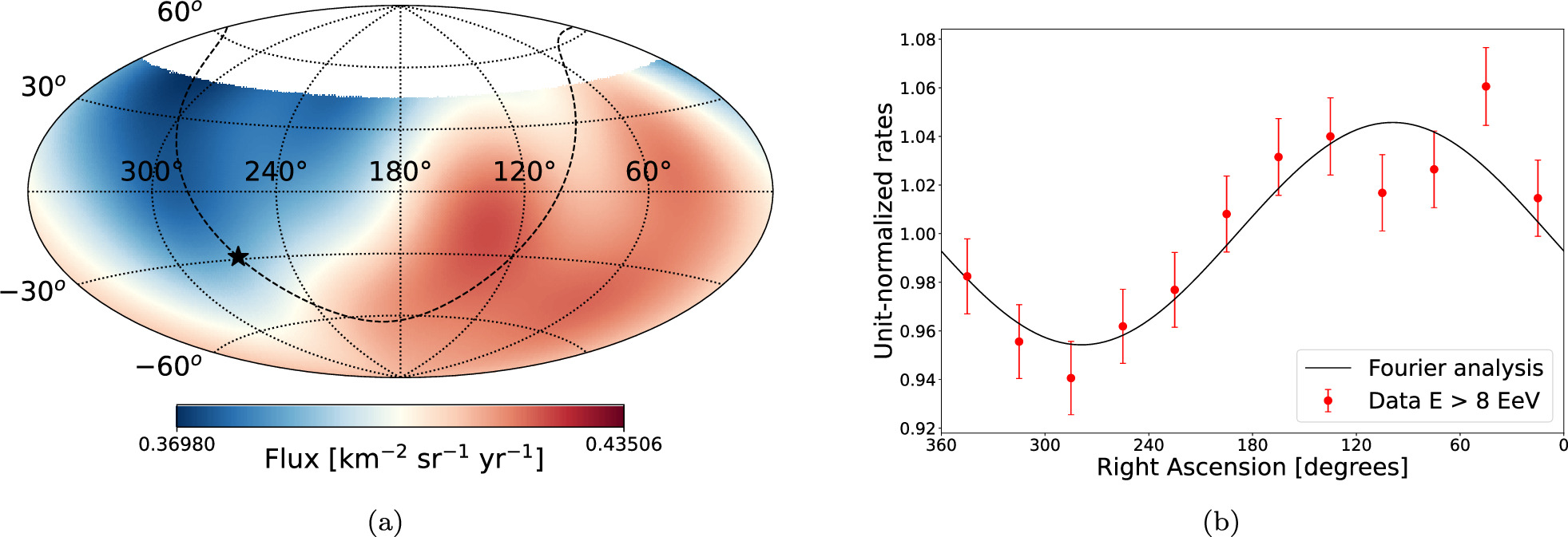
Figure 1. (a) Flux above 8 EeV, smoothed by a Fisher distribution with a mean cosine of the angular distance to the center of the window equal to that of a top-hat distribution with a radius of 45°, in equatorial coordinates. The position of the Galactic center is shown with a star, and the Galactic plane is indicated with a dashed line. (b) Distribution in R.A. of the unit-normalized rates of events with E ≥ 8 EeV. The black line shows the obtained distribution, with the Fourier analysis assuming only a dipolar component.
Download figure:
Standard image High-resolution image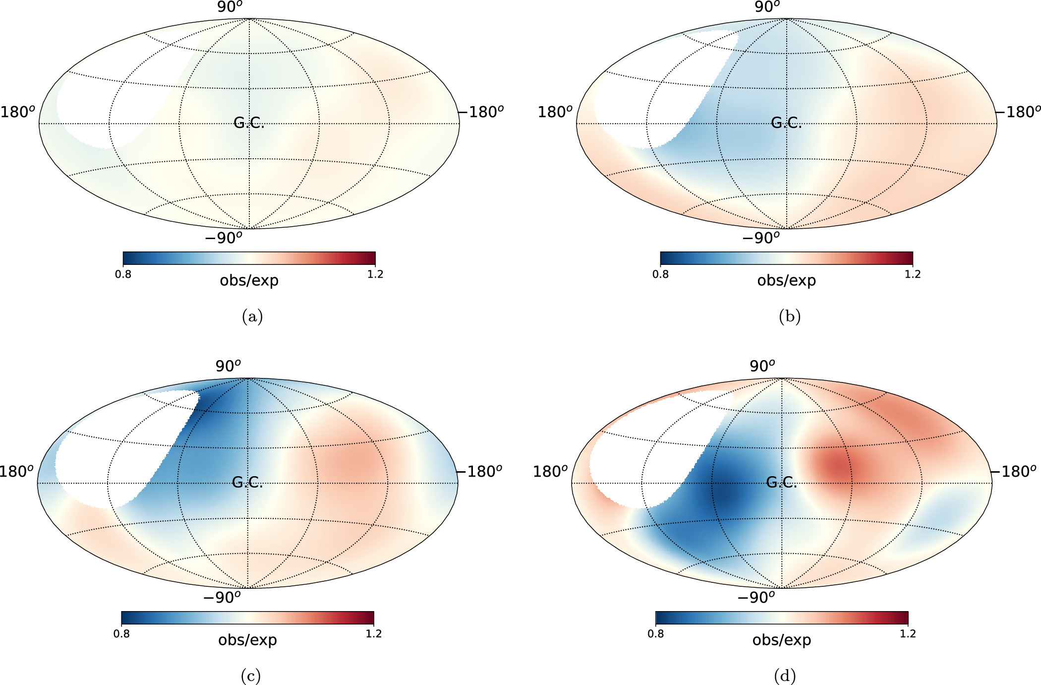
Figure 2. Ratio between the number of observed events and the number expected from an isotropic distribution, in Galactic coordinates, for the (a) 4–8 EeV, (b) 8–16 EeV, (c) 16–32 EeV, and (d) ≥32 EeV energy bins. The smoothing corresponds to a Fisher distribution with a mean cosine of the angular distance to the center of the window equal to that of a top-hat distribution with a radius of 45°.
Download figure:
Standard image High-resolution imageIn Figure 3, the evolution with energy of the dipole direction and amplitude is plotted. A fit to the amplitude as a function of energy,  , is performed obtaining d10 = 0.049 ± 0.009 and β = 0.97 ± 0.21, in agreement with Pierre Auger Collaboration (2018). This growth in amplitude is possibly due to the larger relative contribution from the nearby sources for increasing energies, whose distribution is more inhomogeneous. Another effect that also results in an increase of the dipole amplitude with energy, secondary to this one, is the growth of mean rigidity of the particles, leading to smaller deflections and thus larger dipolar amplitudes (see Section 5 for a comparison of model predictions to data).
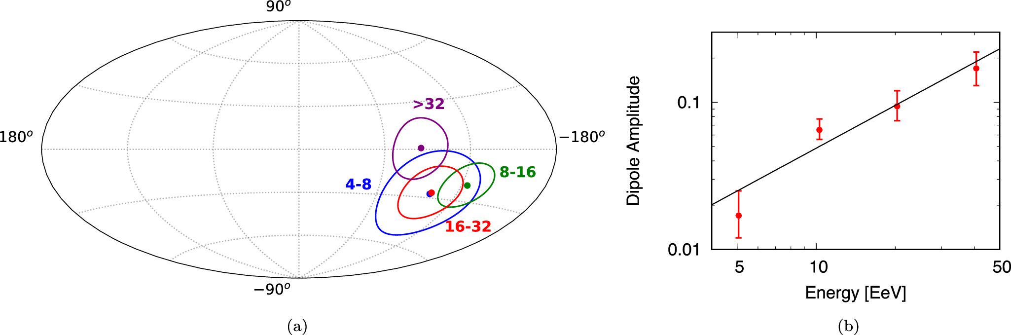
Figure 3. (a) Map with the directions of the 3D dipole for different energy bins, in Galactic coordinates. The contours of equal probability per unit solid angle, marginalized over the dipole amplitude, that contain the 68% CL range are shown. (b) The evolution of the dipole amplitude with energy, for the four energy bins considered: (4–8, 8–16, 16–32, ≥32) EeV.
Download figure:
Standard image High-resolution imageTo show that there are no significant unaccounted-for systematics effects, in Table 2 the solar and antisidereal first-harmonic amplitudes ( and
and  ) and the probability of getting a larger amplitude from fluctuations of an isotropic distribution (
 and
and  ) are reported, for each energy bin in which the Fourier analysis in R.A. was done at the sidereal frequency. The results are compatible with no significant modulation being present at these frequencies. Furthermore, for the Fourier analysis in azimuth, the
  parameters, which measure the east–west modulation, were verified to be compatible with zero (since any flux modulation from the sky should be averaged owing to Earth’s rotation).
Table 2. Solar and Antisidereal First-harmonic Amplitudes,  and
and  , and the Corresponding Isotropic Probabilities,
  and
and  , for Each Energy Bin
| E |

|

|

|

|
|---|---|---|---|---|
| (EeV) | (%) | (%) | ||
| 2–4 |

| 0.18 |

| 0.48 |
| 4–8 |

| 0.28 |

| 0.65 |
| ≥8 |

| 0.91 |

| 0.10 |
| 8–16 |

| 0.71 |

| 0.36 |
| 16–32 |

| 0.29 |

| 0.15 |
| ≥32 |

| 0.83 |

| 0.93 |
Download table as: ASCIITypeset image
The statistics of the E ≥ 8 EeV cumulative energy bin is large enough that the data set can be separated into time-ordered subsets and tested for their stability. The results, dividing the data set into two (the date corresponding to half the data set is 2014 August 19) and four subsets (the dates corresponding to the end of each quarter of the data set being 2010 September 15, 2014 August 19, 2018 September 5, and 2022 December 31), are listed in Table 3. It is seen that the equatorial dipole amplitude and phase are consistent within the statistical uncertainties in the different time periods considered. Given that no time variation of the equatorial dipole modulation is found, an upper limit to its long-term rate of change of 0.003 yr−1 at the 95% CL can be set using a linear fit to the split data, which illustrates the long-term stability of the detector. Another check that was performed was to separate the data set into two zenith angle ranges, larger or smaller than 60°, corresponding to the different reconstructions (vertical and inclined), and the results are compatible with each other.
Table 3. Number of Events (N), Reconstructed Equatorial Dipole Amplitude (d⊥), Phase (αd
), and Isotropic Probability ( ) Separating the Data Set into Time-ordered Subsets for the E ≥ 8 EeV Cumulative Energy Bin
| Time Bins | N | d⊥ | αd |

|
|---|---|---|---|---|
| (%) | (deg) | |||
| 1/2 | 24,839 |

| 100 ± 12 | 1.1 × 10⁻⁵ |
| 2/2 | 24,839 |

| 94 ± 11 | 6.9 × 10⁻⁷ |
| 1/4 | 12,419 |

| 111 ± 15 | 5.6 × 10⁻⁴ |
| 2/4 | 12,420 |

| 87 ± 19 | 1.1 × 10⁻² |
| 3/4 | 12,419 |

| 92 ± 14 | 1.5 × 10⁻⁴ |
| 4/4 | 12,420 |

| 97 ± 17 | 3.8 × 10⁻³ |
Note. The first two rows correspond to separating the data set into two time-ordered bins, while the following rows correspond to separating the data set into four time-ordered bins.
Download table as: ASCIITypeset image
4.2. 3D Dipole and Quadrupole above 4 EeV
In Table 4, the results obtained if a quadrupolar component is included in the Fourier analysis for each energy bin are shown. The dipole components
d
= (dx
, dy
, dz
), the five independent quadrupolar components Qij
, the quadrupole amplitude  , and the 99% CL upper limits QUL are listed. It is seen that the quadrupolar components are not significant and that the dipole components are consistent with the results we obtain assuming only a dipole.
Table 4. Results Obtained Considering Both Dipolar and Quadrupolar Components
| 4–8 EeV | ≥8 EeV | 8–16 EeV | 16–32 EeV | ≥32 EeV | |
|---|---|---|---|---|---|
| dx | −0.003 ± 0.007 | −0.002 ± 0.011 | −0.002 ± 0.012 | 0.029 ± 0.024 | −0.1 ± 0.5 |
| dy | 0.005 ± 0.007 | 0.059 ± 0.011 | 0.048 ± 0.012 | 0.088 ± 0.024 | 0.1 ± 0.5 |
| dz | 0.002 ± 0.019 | −0.02 ± 0.03 | 0.02 ± 0.04 | −0.15 ± 0.07 | −0.23 ± 0.13 |
| Qzz | 0.03 ± 0.03 | 0.04 ± 0.05 | 0.10 ± 0.06 | −0.13 ± 0.13 | −0.16 ± 0.25 |
| Qxx − Qyy | 0.018 ± 0.025 | 0.07 ± 0.04 | 0.03 ± 0.04 | 0.18 ± 0.08 | 0.30 ± 0.17 |
| Qxy | −0.016 ± 0.012 | 0.026 ± 0.019 | 0.041 ± 0.022 | −0.05 ± 0.04 | 0.11 ± 0.08 |
| Qxz | −0.010 ± 0.016 | 0.017 ± 0.025 | 0.003 ± 0.029 | 0.10 ± 0.06 | −0.10 ± 0.10 |
| Qyz | −0.019 ± 0.016 | 0.005 ± 0.025 | −0.029 ± 0.029 | 0.09 ± 0.06 | 0.13 ± 0.10 |
| Q | 0.018 ± 0.010 | 0.028 ± 0.015 | 0.05 ± 0.02 | 0.10 ± 0.03 | 0.13 ± 0.06 |
| QUL | 0.04 | 0.05 | 0.08 | 0.15 | 0.26 |
Note. For every energy bin, the dipole components d = (dx , dy , dz ), the five independent quadrupolar components Qij , the quadrupole amplitude Q, and the 99% CL upper limit QUL are presented. The x-axis is chosen along the α = 0 direction.
Download table as: ASCIITypeset image
4.3. Angular Power Spectrum above 4 EeV
The measured power spectra for different energy bins are presented in Figure 4. The gray band, obtained from Monte Carlo simulations, corresponds to the 99% CL interval that would result from fluctuations of isotropic distributions. This band was constructed by performing 50,000 isotropic simulations, each containing the same number of events as the data. The  and
and  obtained for all energy bins are consistent with the results from the previous Sections 4.1 and 4.2 using a Fourier analysis. Besides the significant dipolar pattern corresponding to
  , the only
  values that stand above the 99% CL of isotropic fluctuations are
  , corresponding to an angular scale of ∼180°/ℓ ≈ 11°, and
  , corresponding to an angular scale of ∼23°, for the energy bins of (4, 8) EeV and (16, 32) EeV, respectively. After statistical penalization for searches over different multipoles and energy bins (four independent energy bins × 20 multipole measurements = 80), the probabilities of these results arising from fluctuations of isotropy are 3.3% and 26.5%, respectively. All other
  values in different energy bins are not significant.
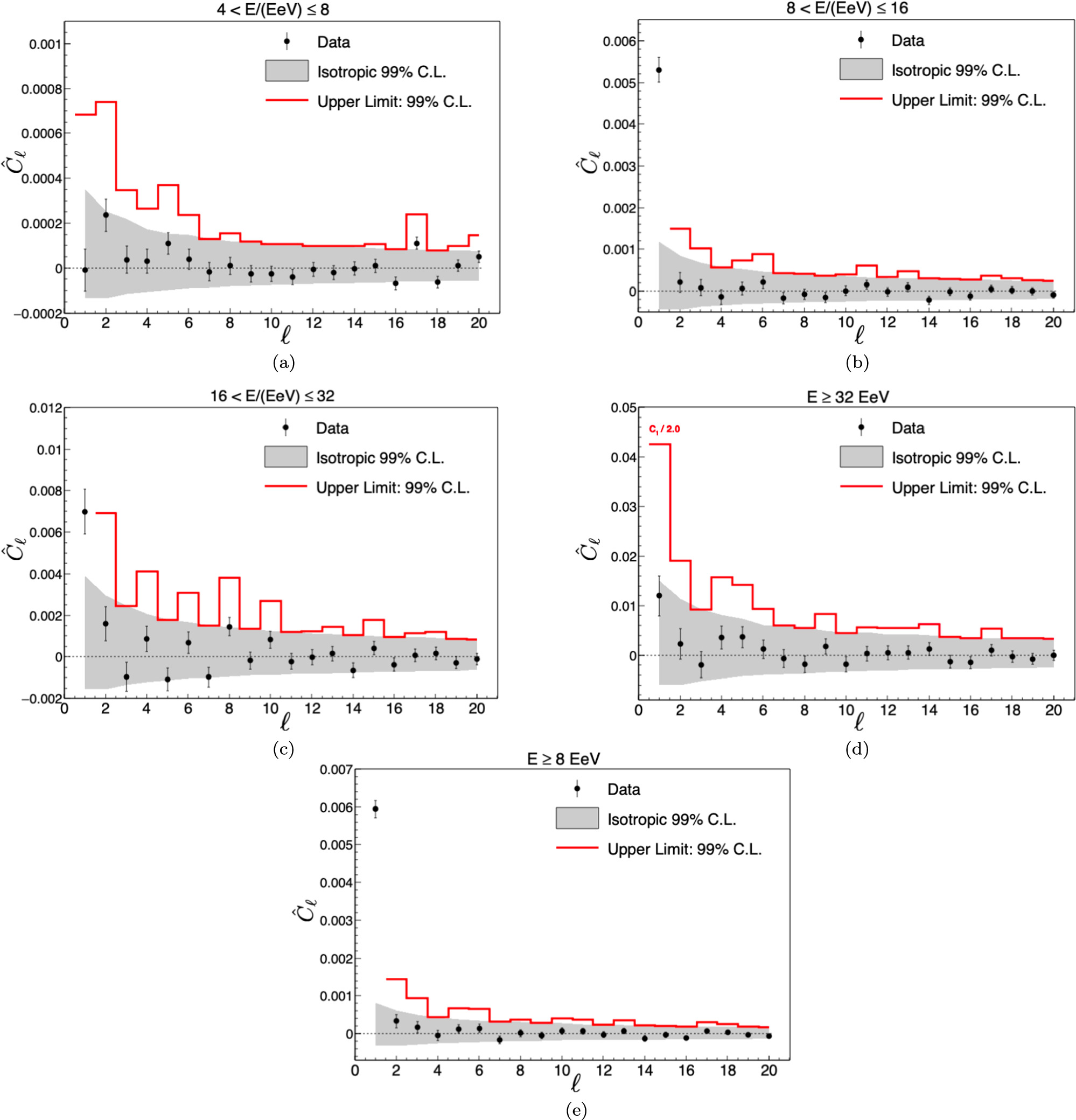
Figure 4. Angular power spectrum measurements for the (a) 4–8 EeV, (b) 8–16 EeV, (c) 16–32 EeV, (d) ≥32 EeV, and (e) ≥8 EeV energy bins. The gray bands correspond to the 99% CL fluctuations that would result from an isotropic distribution. The red lines correspond to the 99% CL upper limits. In panel (d), the upper limit  has been divided by 2 to maintain the visibility of other features in the plot.
Download figure:
Standard image High-resolution imageThe red lines indicate the upper limits on multipole amplitudes with 99% CL. They were obtained by using the following approach. For each possible amplitude Cℓ
, the probability of reconstructing  given a true value of Cℓ
, p
given a true value of Cℓ
, p
 is estimated from simulations. For this, cosmic-ray skies were simulated by drawing events according to an underlying anisotropic distribution corresponding to Cℓ
, considering an observatory with relative exposure W. The underlying anisotropic distribution is achieved by generating aℓ
m
coefficients uniformly distributed on the surface of a (2ℓ + 1)-dimensional hypersphere of radius
is estimated from simulations. For this, cosmic-ray skies were simulated by drawing events according to an underlying anisotropic distribution corresponding to Cℓ
, considering an observatory with relative exposure W. The underlying anisotropic distribution is achieved by generating aℓ
m
coefficients uniformly distributed on the surface of a (2ℓ + 1)-dimensional hypersphere of radius  . The reconstructed
  for each simulated cosmic-ray sky are obtained using Equation (9). The amplitude
  such that
 is the relevant upper limit.
100
is the relevant upper limit.
100
4.4. Modulation in R.A. Down to 0.03 EeV
The modulation in R.A. is studied for energies below 4 EeV using the data of the SD-1500 and SD-750 arrays, with the East–West method or a Fourier analysis, as described in Section 3.4. The results of these analyses, the equatorial amplitude (d⊥), phase (αd
), and isotropic probability ( ), are presented in Table 5, where it is indicated which method was used in each energy bin. The 99% CL upper limit,
  , is reported. These upper limits are derived from the distribution for a dipolar anisotropy of unknown amplitude, marginalized over the dipole phase, as described in Pierre Auger Collaboration (2020a). In Figure 5, the results are shown, also including those obtained at lower energies by the IceCube and KASCADE-Grande Collaborations (IceCube Collaboration 2012, 2016; KASCADE-Grande Collaboration 2019).
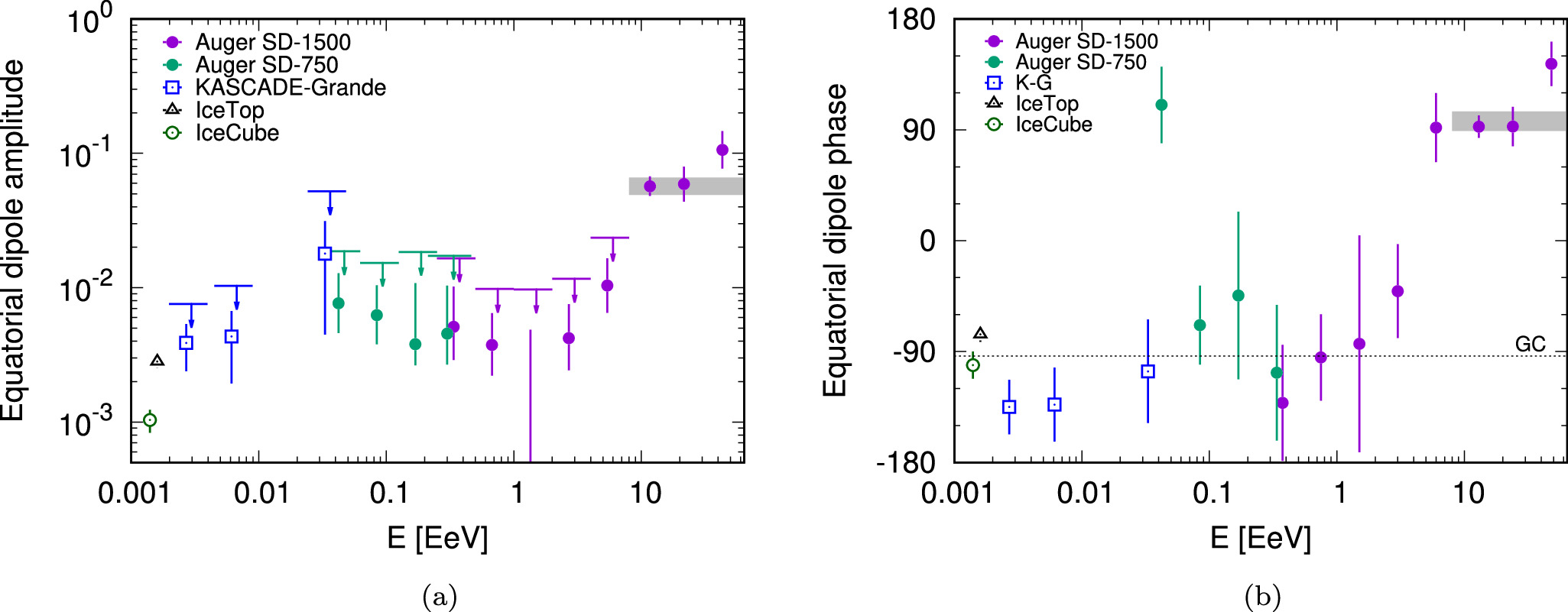
Figure 5. Equatorial dipole (a) amplitude and (b) phase for the energy bins where the data set from the SD-1500 array (purple circles) or that from the SD-750 array (green circles) is used. The 99% CL upper limits for the energy bins in which the obtained amplitude has a P( ) > 1% are shown. Results from the IceCube and KASCADE-Grande Collaborations are also included for comparison (IceCube Collaboration 2012, 2016; KASCADE-Grande Collaboration 2019).
Download figure:
Standard image High-resolution imageTable 5. Results for the Large-scale Analysis in R.A
| E | N | d⊥ | αd |

|

| ||
|---|---|---|---|---|---|---|---|
| (EeV) | (%) | (deg) | |||||
| SD-750 | East–West | 1/32–1/16 | 1,811,897 |

| 110 ± 31 | 0.22 | 1.9 |
| 1/16–1/8 | 1,843,507 |

| −69 ± 32 | 0.23 | 1.5 | ||
| 1/8–1/4 | 607,690 |

| −44 ± 68 | 0.79 | 1.8 | ||
| Fourier | 0.25–0.5 | 135,182 |

| −107 ± 55 | 0.65 | 1.7 | |
| SD-1500 | East–West | 0.25–0.5 | 930,942 |

| −132 ± 47 | 0.51 | 1.7 |
| 0.5–1 | 3,049,342 |

| −95 ± 35 | 0.28 | 1.0 | ||
| 1–2 | 1,639,139 |

| −84 ± 88 | 0.93 | 1.0 | ||
| Fourier | 2–4 | 380,491 |

| −41 ± 38 | 0.36 | 1.2 | |
Note. For each energy bin, the number of events N, the equatorial component of the amplitude d⊥, the R.A. of the dipole direction αd
, the probability of getting a larger amplitude from fluctuations of an isotropic distribution  , and the 99% CL upper limit
  are presented.
Download table as: ASCIITypeset image
Due to the small amplitudes (<1%) and the current amount of statistics, the results listed in Table 5 are not statistically significant ( ), and it is not yet possible to draw firm conclusions. Nonetheless, it is suggestive that the amplitudes of the equatorial dipole increase as a function of energy, from below 1% to above 10%, and that the phases shift from close to the Galactic center to the opposite direction. These changes in amplitude and phase could suggest a transition of the origin of the anisotropies from Galactic cosmic rays to extragalactic ones. Another explanation for these changes could be the impact of the Galactic magnetic field on an extragalactic flux, as discussed in Section 5.
5. Model Predictions and Discussion
Possible explanations of the origin of the dipole measured above 8 EeV assume an inhomogeneous distribution of sources, probably following the large-scale structure distribution in our neighborhood (D. Harari et al. 2014, 2015; P. G. Tinyakov & F. R. Urban 2015; N. Globus & T. Piran 2017; A. di Matteo & P. Tinyakov 2018; C. Ding et al. 2021; D. Allard et al. 2022; T. Bister & G. R. Farrar 2024), or that UHECRs originate from a dominant local source and propagate diffusively through intergalactic magnetic fields (M. Giler et al. 1980; V. S. Berezinskii et al. 1990; S. Mollerach & E. Roulet 2019). The resulting dipole amplitude and direction as a function of energy depend on the source distribution, intervening magnetic fields, and the spectrum and mass composition of the UHECRs. If the sources were distributed like galaxies and if deflections in the Galactic magnetic field could be neglected, a dipolar cosmic-ray anisotropy would be expected in a direction close to that of the dipole associated with the galaxies themselves (P. Erdogdu et al. 2006). On average, a smaller dipolar anisotropy is expected for larger source densities or for more isotropically distributed sources. The amplitude is predicted to grow for increasing energies as a consequence of the shrinking of the horizon due to interactions with the radiation backgrounds (resulting in a larger contribution of the nearby nonhomogeneously distributed sources). Moreover, the Galactic magnetic field modifies the direction and amplitude of the dipolar anisotropy observed at Earth with respect to that of the particles reaching the halo (D. Harari et al. 2010; Pierre Auger Collaboration 2018). These effects depend on the rigidity of the incoming particles and usually lead to a decrease in the dipolar amplitude and also affect the higher multipoles. In particular, for sources following the distribution of galaxies and considering a mean rigidity of the cosmic rays above 8 EeV compatible with the measured mass composition, the direction of the expected dipole would be transformed at Earth after the deflections in the Galactic magnetic field to a direction closer to the observed dipole direction (Pierre Auger Collaboration 2017c).
The energy spectrum and mass composition data measured with the Pierre Auger Observatory above 6 × 10¹⁷ eV can be described by a model with two populations of sources, dominating the flux above and below a few EeV, respectively (Pierre Auger Collaboration 2023a). It has been shown that the data can be well reproduced if the high-energy extragalactic population emits a mixture of heavy and intermediate-mass nuclei with a very hard spectrum and a small rigidity cutoff, while the low-energy component is a mixture of light and intermediate-mass nuclei with a soft spectrum.
In this work, the expected dipole amplitude as a function of energy and the expected directions at Earth are computed for sources emitting cosmic rays according to the best-fitting model for the high-energy population in Pierre Auger Collaboration (2023a) and distributed following the galaxies detected in infrared (IR) in the Two Micron All Sky Survey (2MASS) catalog (M. F. Skrutskie et al. 2006) described in Pierre Auger Collaboration (2022) (with distances from the HyperLEDA database; D. Makarov et al. 2014). The expectation for the dipole amplitude is calculated in the four energy bins above 4 EeV for a population of equal-luminosity sources with number density 10−5 and 10−4 Mpc−3 selected randomly from a volume-limited sample of the IR catalog up to 120 Mpc (and from a uniform distribution for larger distances and in the region of the Galactic plane mask). The sources are considered to emit a mixed composition of particles with spectrum E2 with a rigidity cutoff Rcut = 1018.15 eV (Pierre Auger Collaboration 2023a). The fraction of the total source emissivity above 1017.8 eV in each mass group is (IH, IHe, IN, ISi, IFe) = (0., 0.236, 0.721, 0.013, 0.031) (Pierre Auger Collaboration 2023a). The particles were propagated taking into account the interactions with the extragalactic background radiation as described by the Gilmore et al. model (R. C. Gilmore et al. 2012) using the SimProp propagation code (R. Aloisio et al. 2017). The arrival direction of the particles at the halo was mapped to the arrival direction at Earth taking into account the deflection in the regular Galactic magnetic field according to the rigidity of the particles and considering for reference the field model from R. Jansson & G. R. Farrar (2012). The dipole direction before magnetic deflections for the whole IR catalog up to 120 Mpc is (l, b) = (255°, 50°).
In Figure 6 the direction of the mean dipole of the simulations and the 68% CL sky region obtained for 103 realizations of the source distribution for a density of 10−4 Mpc−3 are presented. The results for a source density of 10−5 Mpc−3 are similar, but the contour regions are larger owing to the larger fluctuations in the source distribution. 101 In the left panel of Figure 7 the median and 68% CL range of the dipole amplitudes are shown for the two source densities considered, also including for comparison the results from data. The expected values of the average quadrupole amplitude, Q, for the same models of the high-energy source population are displayed in the right panel of Figure 7, together with the results from data and the 99% CL upper limits obtained for Q. The dipolar and quadrupolar anisotropies for both source densities are compatible with the experimental results within the uncertainties, although for the smallest source density the quadrupole prediction is in slight tension, in particular for the highest energy bin. Possible ways to reduce the quadrupole prediction, besides increasing the source density considered, would be to invoke strong turbulent Galactic and/or extragalactic magnetic field deflections to smooth out the arrival direction maps (D. Allard et al. 2022; T. Bister & G. R. Farrar 2024).
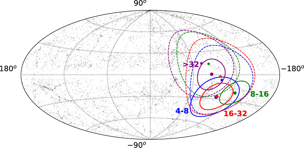
Figure 6. Map in Galactic coordinates showing the predictions for the direction of the mean dipole (stars) and the 68% CL contour regions (dashed lines) obtained for 103 realizations of the source distribution for a density of 10−4 Mpc−3 and for each energy bin above 4 EeV. This is compared to what is obtained in data (solid lines). The gray dots represent the location of the galaxies in the IR catalog within 120 Mpc.
Download figure:
Standard image High-resolution image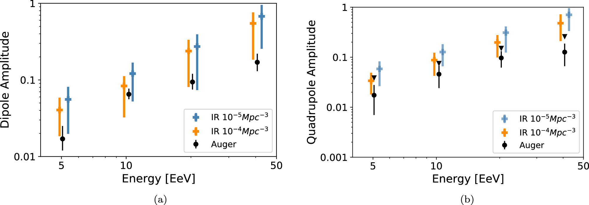
Figure 7. (a) Median and 68% CL range of the dipole amplitudes for the two source densities considered, 10−4 Mpc−3 (orange) and 10−5 Mpc−3 (blue). (b) Expected values of the average quadrupole amplitude, Q, for the same model of the high-energy population of sources. In both panels the results from data are shown (black circles), and for the average quadrupole amplitude the 99% CL upper limits are included (black triangles). The four energy ranges are (4–8, 8–16, 16–32, ≥32) EeV.
Download figure:
Standard image High-resolution imageFor energies below the ankle, the results for the low-energy component of the combined fit of the energy spectrum and mass composition measured with the Pierre Auger Observatory can be described by two different scenarios (Pierre Auger Collaboration 2023a). The first one consists of a Galactic contribution of nitrogen and an extragalactic contribution of protons (which could be produced by interactions of nuclei from the high-energy population in the environment of the sources). The second one consists of an extragalactic contribution of mixed composition (proton, helium, and nitrogen). In both scenarios, there is also a high-energy extragalactic component with mixed composition, as considered before.
The dipolar anisotropy of the nitrogen Galactic component of the first scenario is expected to point close to the Galactic center, in agreement with the measured R.A. phase at low energies, although its amplitude may be close to the present upper bounds at EeV energies (Pierre Auger Collaboration 2012).
Regarding the second scenario, the arrival direction distribution of cosmic rays from the lower-energy extragalactic component is expected to be more isotropic, since at those energies cosmic rays can reach Earth from distances larger than 1 Gpc and the distribution of matter in the Universe at very large scales looks quite uniform. However, even in the case of a perfectly uniform distribution of cosmic rays in some reference frame outside the galaxy, the distribution of arrival directions at Earth is not expected to be isotropic. In particular, the relative motion of the observer with respect to the isotropic reference frame gives rise to an anisotropy that is expected to be dipolar before traversing the Galactic magnetic field, the so-called Compton−Getting effect. If the isotropic reference frame is taken as that of the cosmic microwave background (CMB), this dipolar anisotropy amplitude has been estimated to be of order 6 × 10⁻³ (M. Kachelriess & P. D. Serpico 2006), pointing in the direction of the CMB dipole, (l, b) = (264°, 48°) (Planck Collaboration et al. 2020). This amplitude is an order of magnitude smaller than the measured anisotropies at the highest energies and thus represents a subdominant effect above the ankle, but it is of the order of the anisotropies measured below the ankle. The propagation in the Galactic magnetic field distorts the dipolar pattern, changing the amplitude and direction of the dipole observed at Earth, which can have a notable effect on the predictions for the R.A. phase (S. Mollerach et al. 2022). In particular, the dipole direction may shift below a few EeV toward the inner spiral arm direction, at (l, b) ≃ (−100°, 0°), which can be relevant to explain the observed change in phase. In addition, as a consequence of the Galaxy rotation, the Galactic magnetic field has a small electric component that leads to a direction-dependent cosmic-ray acceleration, possibly affecting the anisotropies at a level comparable to the Compton−Getting effect (S. Mollerach et al. 2022).
Clearly, more precise measurements of the anisotropies in the energy range from 0.1 EeV to a few EeV, possibly discriminated by mass composition, and a better knowledge of the Galactic magnetic field will be very useful to shed light on the origin of the cosmic rays below the ankle and on the details of the Galactic-to-extragalactic transition.
6. Conclusions
The results of the anisotropy searches using the arrival directions of UHECRs detected in Phase 1 of operation of the Pierre Auger Observatory, corresponding to the 19 yr of data gathered before the implementation of the AugerPrime upgrade, were presented. The significance of the established equatorial dipole for the cumulative energy bin above 8 EeV is now 6.8σ, and that for the bin 8–16 EeV is 5.7σ, surpassing the discovery level. For the ≥8 EeV cumulative energy bin, the statistics are such that we can divide the data set into time-ordered bins, and we find no time variation of the equatorial dipole modulation with an upper limit on the long-term rate of change of 0.003 yr−1 at the 95% CL. If a quadrupolar distribution is allowed in the flux parameterization, the obtained quadrupolar moments are not statistically significant.
The dipole amplitudes increase with energy above 4 EeV. Model predictions were presented for sources following the distribution of galaxies, assuming a source density of 10−5 Mpc−3 or 10−4 Mpc−3, and emitting according to the model for the high-energy population from our combined fit of spectrum and composition (Pierre Auger Collaboration 2023a). The predictions for the dipole amplitude and direction were shown, as well as for the quadrupole amplitude, which are consistent with data within their uncertainties, although some tension with the small observed quadrupole amplitudes seems to be present, in particular for the lowest source density considered and the highest energy bin.
By studying the R.A. distribution of the events, the equatorial component of the dipole down to 0.03 EeV was computed. For energies below 4 EeV the amplitudes are below 1%, compatible with isotropic expectations. However, in most of the energy bins the phase points are consistently close to the Galactic center phase and nearly opposite to the Galactic center phase at energies above 4 EeV. This could be due to the observed anisotropy having a predominant Galactic origin below 1 EeV and a predominant extragalactic origin above a few EeV. Alternatively, this could be caused by the effects of the Galactic magnetic field on an extragalactic flux.
The encouraging prospects of obtaining mass composition estimators on an event-by-event basis with AugerPrime, as well as improved mass estimators with Phase 1 data, will give more information about these anisotropies. An analysis including these estimators to study the different dipole amplitudes obtained by separating the “lighter” and “heavier” events with the present data set is forthcoming.
Acknowledgments
The successful installation, commissioning, and operation of the Pierre Auger Observatory would not have been possible without the strong commitment and effort from the technical and administrative staff in Malargüe. We are very grateful to the following agencies and organizations for financial support:
Argentina—Comisión Nacional de Energía Atómica; Agencia Nacional de Promoción Científica y Tecnológica (ANPCyT); Consejo Nacional de Investigaciones Científicas y Técnicas (CONICET); Gobierno de la Provincia de Mendoza; Municipalidad de Malargüe; NDM Holdings and Valle Las Leñas; in gratitude for their continuing cooperation over land access; Australia—the Australian Research Council; Belgium—Fonds de la Recherche Scientifique (FNRS); Research Foundation Flanders (FWO), Marie Curie Action of the European Union grant No. 101107047; Brazil—Conselho Nacional de Desenvolvimento Científico e Tecnológico (CNPq); Financiadora de Estudos e Projetos (FINEP); Fundação de Amparo à Pesquisa do Estado de Rio de Janeiro (FAPERJ); São Paulo Research Foundation (FAPESP) grant Nos. 2019/10151-2, 2010/07359-6, and 1999/05404-3; Ministério da Ciência, Tecnologia, Inovações e Comunicações (MCTIC); Czech Republic—GACR 24-13049S, CAS LQ100102401, MEYS LM2023032, CZ.02.1.01/0.0/0.0/16 013/0001402, CZ.02.1.01/0.0/0.0/18 046/0016010, CZ.02.1.01/0.0/0.0/17 049/0008422, and CZ.02.01.01/00/22 008/0004632; France—Centre de Calcul IN2P3/CNRS; Centre National de la Recherche Scientifique (CNRS); Conseil Régional Ile-de-France; Département Physique Nucléaire et Corpusculaire (PNC-IN2P3/CNRS); Département Sciences de l’Univers (SDU-INSU/CNRS); Institut Lagrange de Paris (ILP) grant No. LABEX ANR-10-LABX-63 within the Investissements d’Avenir Programme grant No. ANR-11-IDEX-0004-02; Germany—Bundesministerium für Bildung und Forschung (BMBF); Deutsche Forschungsgemeinschaft (DFG); Finanzministerium Baden-Württemberg; Helmholtz Alliance for Astroparticle Physics (HAP); Helmholtz-Gemeinschaft Deutscher Forschungszentren (HGF); Ministerium für Kultur und Wissenschaft des Landes Nordrhein-Westfalen; Ministerium für Wissenschaft, Forschung und Kunst des Landes Baden-Württemberg; Italy—Istituto Nazionale di Fisica Nucleare (INFN); Istituto Nazionale di Astrofisica (INAF); Ministero dell’Università e della Ricerca (MUR); CETEMPS Center of Excellence; Ministero degli Affari Esteri (MAE), ICSC Centro Nazionale di Ricerca in High Performance Computing, Big Data and Quantum Computing, funded by European Union NextGenerationEU, reference code CN 00000013; México—Consejo Nacional de Ciencia y Tecnología (CONACYT) No. 167733; Universidad Nacional Autónoma de México (UNAM); PAPIIT DGAPA-UNAM; the Netherlands—Ministry of Education, Culture and Science; Netherlands Organisation for Scientific Research (NWO); Dutch national e-infrastructure with the support of SURF Cooperative; Poland—Ministry of Education and Science, grant Nos. DIR/WK/2018/11 and 2022/WK/12; National Science Centre, grant Nos. 2016/22/M/ST9/00198, 2016/23/B/ST9/01635, 2020/39/B/ST9/01398, and 2022/45/B/ST9/02163; Portugal—Portuguese national funds and FEDER funds within Programa Operacional Factores de Competitividade through Fundação para a Ciência e a Tecnologia (COMPETE); Romania—Ministry of Research, Innovation and Digitization, CNCS-UEFISCDI, contract No. 30N/2023 under Romanian National Core Program LAPLAS VII, grant No. PN 23 21 01 02 and project No. PN-III-P1-1.1-TE-2021-0924/TE57/2022, within PNCDI III; Slovenia—Slovenian Research Agency, grants P1-0031, P1-0385, I0-0033, N1-0111; Spain—Ministerio de Ciencia e Innovación/Agencia Estatal de Investigación (PID2019-105544GB-I00, PID2022-140510NB-I00, and RYC2019-027017-I), Xunta de Galicia (CIGUS Network of Research Centers, Consolidación 2021 GRC GI-2033, ED431C-2021/22, and ED431F-2022/15), Junta de Andalucía (SOMM17/6104/UGR and P18-FR-4314), and the European Union (Marie Sklodowska-Curie 101065027 and ERDF); USA—Department of Energy, contract Nos. DE-AC02-07CH11359, DE-FR02-04ER41300, DE-FG02-99ER41107, and DE-SC0011689; National Science Foundation, grant Nos. 0450696 and NSF-2013199; the Grainger Foundation; Marie Curie-IRSES/EPLANET; European Particle Physics Latin American Network; and UNESCO.
Footnotes
- 97
Due to the smaller statistics of Telescope Array (∼10 times smaller), a large-scale dipolar anisotropy has not been confirmed in their data set, with a 99% CL upper limit on the first-harmonic amplitude of 7.3% (Telescope Array Collaboration 2020).
- 98
For the source model that best fits the spectrum and composition results obtained in Pierre Auger Collaboration (2023a), the cosmic-ray horizon is shrunk from a few hundreds of megaparsecs to a few tens of megaparsecs between 10 and 100 EeV, and the mean rigidity changes from ∼4 to ∼8 EV in the same energy range.
- 99
In Pierre Auger Collaboration (2017a), unlike in this work, the results were presented without removing the noise term. Thus, by construction, in this work the average of the isotropic simulations is zero, and any particular realization with a negative Cℓ is interpreted as a statistical fluctuation consistent with isotropy.
- 100
Since this procedure can lead to upper limits tighter than the upper bounds obtained from isotropy with 99% CL,
 , when the measured values of are smaller than the expected average for isotropy, the upper limits presented are defined as
in order to cope with this undesired behavior.
, when the measured values of are smaller than the expected average for isotropy, the upper limits presented are defined as
in order to cope with this undesired behavior. - 101
Note that backtracking studies in the UF23 GMF models (M. Unger & G. R. Farrar 2024), including also a turbulent component, show that the direction of the dipole of cosmic rays with E/Z = 1 EeV having a dipolar distribution with maximum in the direction of the 2MRS dipole outside the Galaxy has, after traversing the Galactic magnetic field, a median angular separation of 17
5 (or 15


