Abstract
Fragmentation contributes to the formation and evolution of stars. Observationally, high-mass stars are known to form multiple-star systems, preferentially in cluster environments. Theoretically, Jeans instability has been suggested to determine characteristic fragmentation scales, and thermal or turbulent motion in the parental gas clump mainly contributes to the instability. To search for such a characteristic fragmentation scale, we have analyzed Atacama Large Millimeter/submillimeter Array (ALMA) 1.33 mm continuum observations toward 30 high-mass star-forming clumps taken by the Digging into the Interior of Hot Cores with ALMA survey. We have identified 573 cores using the dendrogram algorithm and measured the separation of cores by using the Minimum Spanning Tree technique. The core separation corrected by projection effects has a distribution peaked around 5800 au. In order to remove biases produced by different distances and sensitivities, we further smooth the images to a common physical scale and perform completeness tests. Our careful analysis finds a characteristic fragmentation scale of ∼7000 au, comparable to the thermal Jeans length of the clumps. We conclude that thermal Jeans fragmentation plays a dominant role in determining the clump fragmentation in high-mass star-forming regions, without the need to invoke turbulent Jeans fragmentation.
Original content from this work may be used under the terms of the Creative Commons Attribution 4.0 licence. Any further distribution of this work must maintain attribution to the author(s) and the title of the work, journal citation and DOI.
1. Introduction
Fragmentation plays an important role in the formation of substructures in molecular clouds, leading to star formation. In particular, high-mass stars preferentially form in clustered environments (Lada & Lada 2003) and, therefore, a full understanding of the fragmentation process is key to uncovering how high-mass stars are formed. Turbulent hydrodynamic simulations of clustered star formation have demonstrated that gravitational (thermal Jeans) and turbulent Jeans fragmentation of dense molecular clumps create stellar clusters (e.g., Bonnell et al. 2001; Klessen et al. 1998; Wang et al. 2010; Pelkonen et al. 2021; Vázquez-Semadeni et al. 2019).
For the simplest case in which the thermal pressure balances with self-gravity, the thermal Jeans fragmentation is likely a dominant process of structure formation (e.g., Jeans 1902; Larson 1985). It has a characteristic scale, the so-called Jeans length, which is given by

where  is the 1D isothermal sound speed, G is the gravitational constant, and ρ is the mass density. The parameters kB
, T, μ, and mH are the Boltzmann constant, the gas temperature, the mean molecular weight per free particle (assuming μ = 2.37 from Kauffmann et al. 2008), and the mass of a hydrogen atom, respectively. This length scale can be affected by various factors, such as magnetic fields and external pressure (Larson 1985). For example, the external pressure can make the fragmentation scale shorter by producing surface deformation instabilities (e.g., Chandrasekhar & Fermi 1953). The magnetic fields shorten or lengthen the fragmentation scales, depending on the degree of the dynamical support (e.g., Nagasawa 1987; Nakamura et al. 1993; Das et al. 2021).
is the 1D isothermal sound speed, G is the gravitational constant, and ρ is the mass density. The parameters kB
, T, μ, and mH are the Boltzmann constant, the gas temperature, the mean molecular weight per free particle (assuming μ = 2.37 from Kauffmann et al. 2008), and the mass of a hydrogen atom, respectively. This length scale can be affected by various factors, such as magnetic fields and external pressure (Larson 1985). For example, the external pressure can make the fragmentation scale shorter by producing surface deformation instabilities (e.g., Chandrasekhar & Fermi 1953). The magnetic fields shorten or lengthen the fragmentation scales, depending on the degree of the dynamical support (e.g., Nagasawa 1987; Nakamura et al. 1993; Das et al. 2021).
Turbulent pressure is dominant over the thermal pressure at the clump and cloud scales of ∼0.1–10 pc. In such cases, turbulence supports the clouds and clumps on large scales against gravitational contraction, while it provokes collapse and fragmentation on local scales, by forming overdensities due to the dynamic interaction of turbulent eddies or waves. Bonazzola et al. (1987) derived the turbulent Jeans fragmentation condition by introducing the wavenumber (k) depending on the effective sound speed,

where v(k) is determined by the turbulent power spectrum. For turbulent interstellar clouds, this relation breaks down below ∼10−2 pc scale, at which the thermal pressure becomes comparable to the turbulent pressure, as it has been seen in infrared dark clouds (IRDCs; e.g., Sanhueza et al. 2017, 2019, 2021; Morii et al. 2021, 2023, 2024; Li et al. 2020, 2022, 2023). Therefore, the minimum fragmentation scale in a turbulent medium is likely to be set to that of thermal Jeans fragmentation, that is the thermal Jeans length (see also Vázquez-Semadeni & Gazol 1995). If the dense filaments have a characteristic width of ∼0.1 pc, as suggested by Herschel observations of nearby molecular clouds (Arzoumanian et al. 2011), the characteristic fragmentation scale is suggested to be around 0.3 pc, which corresponds to the wavelength of the most unstable mode (Larson 1985). For high-mass clumps, this filament fragmentation scale appears to be about 10 times larger than the thermal Jeans length (Equation (2)).
Previous studies of core separations suggest the existence of the characteristic length scale. For example, Beuther et al. (2018) observed 20 molecular clumps located in high-decl. regions (>24°) with the IRAM Northern Extended-Millimeter Array (NOEMA) with an angular resolution between ∼032 and ∼0
50 (∼960–1500 au at 3 kpc). They identified 121 cores and measured their separations in each region. They found that most of their separations are distributed under 5000 au. Their core separation takes its peak at around thermal Jeans length.
Lu et al. (2020) studied three high-density clouds in the Central Molecular Zone (CMZ). They used Atacama Large Millimeter/submillimeter Array (ALMA) band 6 (1.33 mm wavelength) with an angular resolution of ∼02, corresponding to ∼1600 au at ∼8.2 kpc. They identified about 800 cores. The thermal Jeans length range is estimated as ∼1.0 × 10⁴ − 1.9 × 10⁴ au. They suggested that the core separations match the thermal Jeans length of ∼0.2 pc with a gas density of 106 cm−3 and temperature of 20–50 K. The CMZ is an extreme environment in the galaxy, and the results in this region may not be applicable to other high-mass star-forming regions, even though their sample size is large.
Zhang et al. (2021) studied eight high-mass starless clumps including four clumps associated with the H II region. Using ALMA with an angular resolution of ∼13 (∼5100 au at ∼4 kpc), they identified 51 cores in eight regions and found two peaks in the separation distribution at
 and
and  . They argued that the existence of two peaks implies hierarchical fragmentation on ≲104 au. However, the shorter peak is almost equal to their beam size. At a similar angular resolution (∼1
2), the ALMA Survey of 70 μm Dark High-mass Clumps in Early Stages (ASHES; Sanhueza et al. 2019; Morii et al. 2021) explains the fragmentation in 12 IRDC clumps Sanhueza et al. (2019) and the complete survey with 39 sources (Morii et al. 2023, 2024) as dominated by thermal Jeans fragmentation rather than turbulent Jeans fragmentation.
These previous studies add to evidence that the thermal Jeans fragmentation is important in high-mass star-forming regions, with a few counterexamples, as the study of the Carina Nebula by Rebolledo et al. (2020). However, the statistics and spatial resolution are still insufficient to conclude that the core separation is comparable to the thermal Jeans length of the parent clumps.
In this work, we present the Digging into the Interior of Hot Cores with ALMA (DIHCA) survey. We have observed 30 high-mass star-forming regions to search for dense compact cores at high-angular resolution in ALMA band 6 (∼226 GHz; ∼1.33 mm). In the DIHCA project, the targets were observed in two configurations providing ∼006 (extended configuration) and ∼0
3 (compact configuration) resolutions. As seen in a case study of DIHCA, cores are clearly resolved at 0
3 angular resolution (Olguin et al. 2021), while at ∼0
06 angular resolution, disk and/or core fragmentation become important (Olguin et al. 2022, 2023; Li et al. 2024). With the aim of exploring clump fragmentation, we determine whether there is a characteristic length scale based on core separations, using the compact configuration data only. An improvement with respect to previous works on this topic is that we put particular emphasis on considering the effects of the different physical resolutions and mass sensitivity among targets when deriving the characteristic core separation for each clump. The analysis of the core/disk fragmentation using the extended configuration data will be presented in a future work (P. Sanhueza et al., 2024, in preparation).
This paper is organized as follows. In Section 2, we describe the target selection. In Section 3, we summarize the observational parameters. We present the results of the 1.33 mm dust continuum observations in Section 4. DIHCA data reveal that the target clumps contain a large number of compact structures, i.e., dense cores. Applying the dendrogram technique, we identify dense cores and derive their physical properties. In Section 5 we discuss the characteristic fragmentation scale and possible biases in the analysis. Finally, we summarize the main results in Section 6.
2. Source Selection
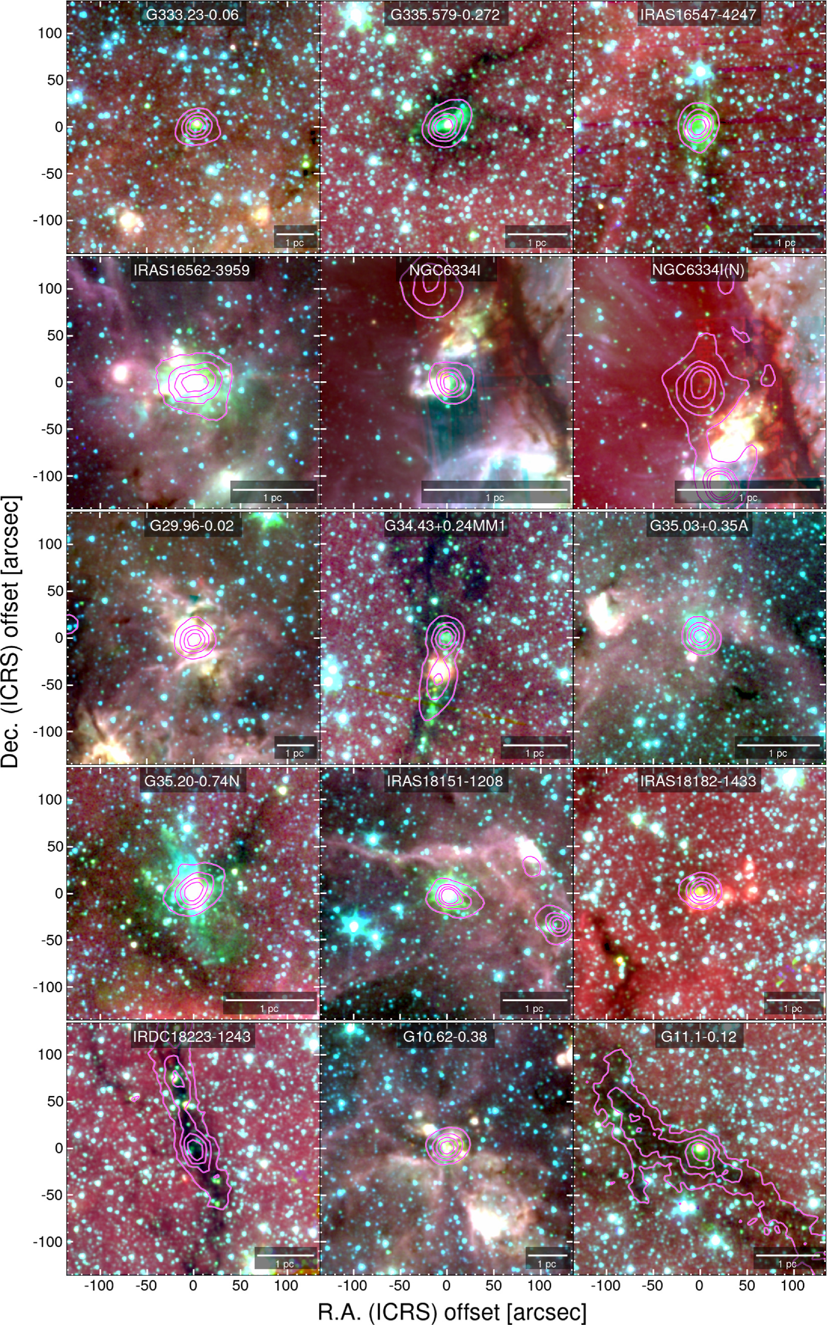
Target sources are selected from the literature according to the following criteria: (i) the target must be bright, (ii) relatively close, and (iii) the clump must have the potential to form high-mass stars. We selected 30 regions whose parameters are summarized in Table 1. In Figure 1, we show the Spitzer/IRAC three-color images (3.6 μm in blue, 4.5 μm in green, and 8.0 μm in red) 10 of the targets with overlaid contours of the dust continuum emission from single-dish telescopes (APEX and James Clerk Maxwell Telescope, JCMT).
Download figure:
Standard image High-resolution image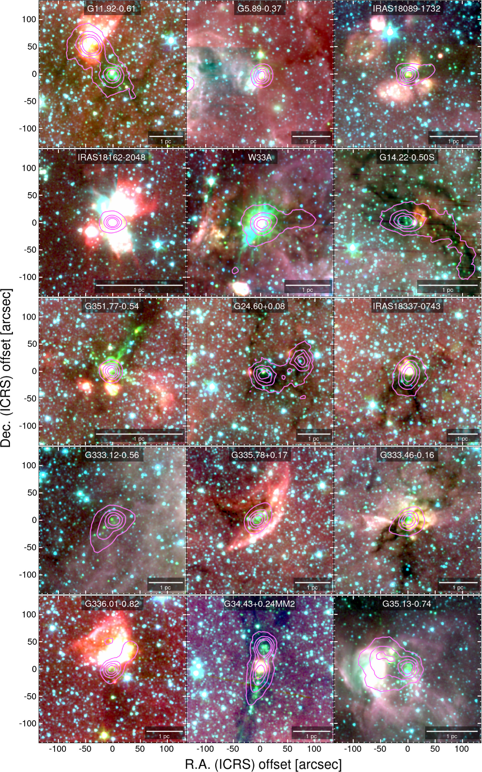
Figure 1. Large-scale overview Spitzer/IRAC three-color image as a background (3.6 μm in blue, 4.5 μm in green, and 8.0 μm in red) with overlaid ATLASGAL 870 μm dust continuum emission in contours for the entire sample, except IRAS 18151–1208 and IRAS 18161–2048 for which JCMT 850 μm dust continuum emission is used. The contour levels are 0.2, 0.4, 0.6, and 0.8 ×Speak, with Speak equal to the peak flux of 870 or 850 μm emission of each clump.
Download figure:
Standard image High-resolution imageTable 1. Physical Properties of High-mass Star-forming Clumps
| Source | Catalog | Position (ICRS) | Dist. | Tdust | Mcl | Rcl | Σcl(H2) | ncl(H2) | Ref. | |
|---|---|---|---|---|---|---|---|---|---|---|
| Clump | Name | R.A. (h:m:s) | Decl. (d:m:s) | (kpc) | (K) | (M⊙) | (pc) | (g cm−2) | (×106cm−3) | |
| (1) | (2) | (3) | (4) | (5) | (6) | (7) | (8) | (9) | (10) | (11) |
| G333.23-0.06 | AGAL 333.234-00.061 | 16:19:51.20 | −50:15:13.00 | 5.20 | 20.9 | 2030 | 0.24 | 2.3 | 5.0 | 1 |
| G335.579-0.272 | AGAL 335.586-00.291 | 16:30:58.76 | −48:43:54.01 | 3.25 | 23.1 | 1570 | 0.20 | 2.5 | 6.4 | 2 |
| IRAS 16547–4247 | AGAL 343.128-00.062 | 16:58:17.22 | −42:52:07.49 | 2.90 | 28.9 | 1380 | 0.16 | 3.4 | 10.6 | 1 |
| IRAS 16562–3959 | AGAL 345.493 + 01.469 | 16:59:41.63 | −40:03:43.62 | 2.38 | 42.3 | 1090 | 0.22 | 1.5 | 3.7 | 3 |
| NGC 6334I | AGAL 351.416 + 00.646 | 17:20:53.30 | −35:47:00.02 | 1.35 | 30.6 | 720 | 0.07 | 10.2 | 77.6 | 4 |
| NGC 6334I(N) | AGAL 351.444 + 00.659 | 17:20:54.90 | −35:45:10.02 | 1.35 | 21.4 | 2190 | 0.14 | 7.6 | 28.5 | 4 |
| G29.96-0.02 | AGAL 029.954-00.016 | 18:46:03.76 | −02:39:22.60 | 5.26 | 35.5 | 1820 | 0.24 | 2.0 | 4.3 | 5 |
| G34.43 + 0.24MM1 | AGAL 034.411 + 00.234 | 18:53:18.01 | +01:25:25.50 | 3.03 | 22.7 | 1050 | 0.14 | 3.4 | 12.0 | 6 |
| G35.03 + 0.35A | AGAL 035.026 + 00.349 | 18:54:00.65 | +02:01:19.30 | 2.32 | 31.8 | 170 | 0.11 | 1.0 | 5.1 | 4 |
| G35.20-0.74N | AGAL 035.197-00.742 | 18:58:13.03 | +01:40:36.00 | 2.19 | 29.5 | 640 | 0.16 | 1.7 | 5.8 | 4 |
| IRAS 18151–1208 | SCOPEG 018.34 + 01.77 | 18:17:58.17 | −12:07:25.02 | 3.00 | 35.0 | 720 | 0.19 | 1.4 | 3.7 | 7 |
| IRAS 18182–1433 | AGAL 016.586-00.051 | 18:21:09.13 | −14:31:50.58 | 3.58 | 24.7 | 650 | 0.17 | 1.5 | 4.4 | 5 |
| IRDC 18223–1243 | AGAL 018.606-00.074 | 18:25:08.55 | −12:45:23.32 | 3.40 | 13.0 | 660 | 0.22 | 0.9 | 2.0 | 1 |
| G10.62-0.38 | AGAL 010.624-00.384 | 18:10:28.65 | −19:55:49.52 | 4.95 | 31.0 | 5160 | 0.22 | 6.8 | 15.7 | 8 |
| G11.1-0.12 | AGAL 011.107-00.114 | 18:10:28.27 | −19:22:30.92 | 3.00 | 15.8 | 470 | 0.23 | 0.6 | 1.4 | 1 |
| G11.92-0.61 | AGAL 011.917-00.612 | 18:13:58.02 | −18:54:19.02 | 3.37 | 22.8 | 1050 | 0.27 | 1.0 | 1.9 | 5 |
| G5.89-0.37 | AGAL 005.884-00.392 | 18:00:30.43 | −24:04:01.64 | 2.99 | 34.5 | 1280 | 0.14 | 4.1 | 15.0 | 5 |
| IRAS 18089–1732 | AGAL 012.888 + 00.489 | 18:11:51.40 | −17:31:28.52 | 2.34 | 23.4 | 550 | 0.13 | 2.1 | 8.1 | 9 |
| IRAS 18162–2048 | SCOPEG 010.84-02.59 | 18:19:12.20 | −20:47:29.02 | 1.30 | 41.0 | 170 | 0.08 | 1.8 | 12.2 | 10 |
| W33A | AGAL 012.908-00.259 | 18:14:39.40 | −17:52:01.02 | 2.53 | 23.6 | 890 | 0.18 | 1.9 | 5.4 | 11 |
| G14.22-0.50S | AGAL 014.114-00.574 | 18:18:13.00 | −16:57:21.82 | 1.90 | 15.8 | 550 | 0.17 | 1.2 | 3.7 | 1 |
| G351.77-0.54 | AGAL 351.774-00.537 | 17:26:42.53 | −36:09:17.40 | 1.30 | 29.9 | 620 | 0.06 | 9.9 | 80.0 | 1 |
| G24.60 + 0.08 | AGAL 024.633 + 00.152 | 18:35:40.50 | −07:18:34.02 | 3.45 | 15.9 | 450 | 0.22 | 0.6 | 1.6 | 12 |
| IRAS 18337–0743 | AGAL 024.441-00.227 | 18:36:40.82 | −07:39:17.74 | 3.80 | 19.3 | 1310 | 0.31 | 0.9 | 1.5 | 1 |
| G333.12-0.56 | AGAL 333.129-00.559 | 16:21:36.00 | −50:40:50.01 | 3.30 | 16.1 | 2720 | 0.26 | 2.6 | 5.2 | 13 |
| G335.78 + 0.17 | AGAL 335.789 + 00.174 | 16:29:47.00 | −48:15:52.32 | 3.20 | 23.1 | 1200 | 0.20 | 2.0 | 5.0 | 13 |
| G333.46-0.16 | AGAL 333.466-00.164 | 16:21:20.26 | −50:09:46.56 | 2.90 | 24.6 | 870 | 0.17 | 2.0 | 6.0 | 1 |
| G336.01-0.82 | AGAL 336.018-00.827 | 16:35:09.30 | −48:46:48.16 | 3.10 | 21.8 | 950 | 0.15 | 2.7 | 9.3 | 1 |
| G34.43 + 0.24MM2 | AGAL 034.401 + 00.226 | 18:53:18.58 | +01:24:45.98 | 3.03 | 20.5 | 1540 | 0.24 | 1.8 | 3.8 | 6 |
| G35.13-0.74 | AGAL 035.132-00.744 | 18:58:06.30 | +01:37:05.98 | 2.20 | 19.4 | 930 | 0.19 | 1.7 | 4.7 | 1 |
Note. (1), (2) All target clumps except for IRAS 18151–1208 and IRAS 18162–2048 are referred from the Compact Source Catalog by Contreras et al. 2013 & Urquhart et al. 2014 in the ATLASGAL survey, while the rest two targets are by Eden et al. 2019 in SCOPE survey. (3), (4) Phase center of ALMA pointing observation. (5), (11) Target distances are referred from the following. 1: Urquhart et al. (2018), 2: Peretto et al. (2013), 3: Moisés et al. (2011), 4: Wu et al. (2014), 5: Sato et al. (2014), 6: Mai et al. (2023), 7: Brand & Blitz (1993), 8: Sanna et al. (2014), 9: Xu et al. (2011), 10: Añez-López et al. (2020), 11: Immer et al. (2013), 12: Dirienzo et al. (2015), 13: Green & McClure-Griffiths (2011).
A machine-readable version of the table is available.
Download table as: Machine-readable (MRT)Typeset image
The aforementioned three selection criteria are described in detail below:
(i) A flux limit of >0.1 Jy at 230 GHz was imposed to make sure that we would detect compact objects in the most extended configuration (the one providing ∼006 resolution that will be presented in a future work).
(ii) To assure a similar physical resolution (and mass sensitivity), we restricted the distance (d) to lie between 1.6 and 3.8 kpc. However, as parallax distances have been made available over time, some of the observed targets resulted to be closer (1.3 kpc) and farther (5.26 kpc), expanding the whole range of distances (see Table 1 for up-to-date distances).
(iii) Some target fields are evidently forming high-mass stars, based on the detection of free–free emission or the presence of hot cores with a line forest spectra. However, to have uniform selection criteria, we also checked whether the clump masses and surface densities satisfy empirical thresholds for high-mass star formation (e.g.,  by Larson (1981) and
  by Kauffmann & Pillai (2010)).
Clumps masses and radii are obtained as follows. Using the 870 μm and 850 μm emission from the ATLASGAL survey 11 (Schuller et al. 2009) and SCOPE survey 12 (Eden et al. 2019), we first fitted each target with a 2D Gaussian function to derive the integrated flux (Sν ) and size of the clumps. The clump radius, Rcl, is calculated as the geometrical mean of the semiminor and semimajor full width at half maximum (FWHM) deconvolved from the beam. The clump masses are derived as,

where  is the gas-to-dust mass ratio (assumed to be 100), κν
is the dust opacity, and Bν
(Tdust) is the Planck function at the dust temperature Tdust, and at the observed frequency ν (or wavelength λ). We calculate κλ
following
is the gas-to-dust mass ratio (assumed to be 100), κν
is the dust opacity, and Bν
(Tdust) is the Planck function at the dust temperature Tdust, and at the observed frequency ν (or wavelength λ). We calculate κλ
following

Here we adopt β = 1.8 and κ1.33 mm = 0.899 cm2 g−1 corresponding to the opacity of dust grain with thin ice mantles at a gas density of ∼106 cm (Ossenkopf & Henning 1994). We obtain κ870 μm = 1.93 cm2 g−1 and κ850 μm = 2.01 cm2 g−1.
For the dust temperatures, we adopted the values derived from one or two components fitting to the spectral energy distribution. For G35.20-0.74N, we adopted the temperature derived by König et al. (2017). For IRAS 18151–1208 and IRAS 18162–2048, the values by McCutcheon et al. (1995). For the remaining 27 clumps, the values were derived in Urquhart et al. (2018). Based on the above references, we adopted the temperature of the cold component as the clump dust temperature for all clumps.
The surface density, Σcl, peak column density, Npeak, and volume density, ncl, are derived as follows,


respectively, where Speak is peak flux, Ω is the solid angle of the synthesized beam, μH is the mean molecular weight per hydrogen molecule (assumed to be 2.8), and mH is the atomic mass of hydrogen. We summarize the clump of physical quantities in Table 1.
In Figure 2, we plot the DIHCA clumps and compare their properties with several threshold relations for high-mass star formation. Larson’s relation Larson (1981) is given as  and is approximately related to a constant surface density of Σ ∼ 460/π
M⊙ pc−2. Kauffmann & Pillai (2010) give
and is approximately related to a constant surface density of Σ ∼ 460/π
M⊙ pc−2. Kauffmann & Pillai (2010) give  for the formation of high-mass stars. For these empirical relations, the clumps located above the thresholds are likely to form high-mass stars. In fact, the clump volume densities obtained here are high, >105–106 cm−3.
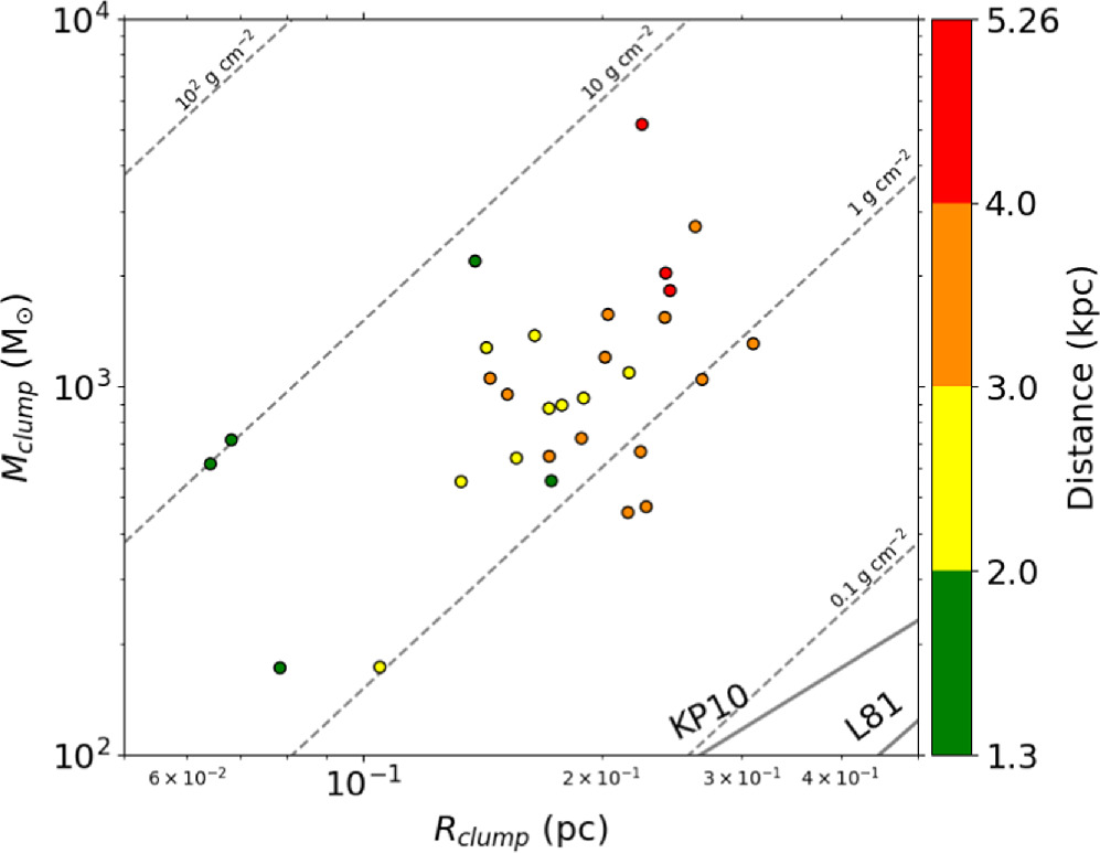
Figure 2. Clump mass against radius. The solid lines show the relationship between Larson (1981, L81) and Kauffmann & Pillai (2010, KP10). All clumps in the sample satisfy the empirical conditions for high-mass star formation. The color coding shows the target distance.
Download figure:
Standard image High-resolution imageA total of 12 of our target clumps were selected from Beltrán & de Wit (2016). Our target list contains both hot cores embedded in infrared dark clouds, known to host the earliest stages of high-mass star formation (e.g., Rathborne et al. 2007; Zhang et al. 2009; Sanhueza et al. 2012, 2013, 2019), as well as massive young stellar objects (MYSOs) presenting the typical hot core line forest with and without signs of compact cm (free–free) emission. See Appendix D for more details on the individual target clumps.
3. Observations and Data Reduction
We observed 30 high-mass star-forming clumps with the ALMA 12 m array, including more than 40 antennas in band 6 (∼226.150 GHz; ∼1.33 mm). Observations were scheduled in Cycles 4, 5, and 6 (Project ID: 2016.1.01036.S, 2017.1.00237.S; PI: Patricio Sanhueza). The angular resolution is ∼03 (∼900 au at 3 kpc) and the maximum recoverable scale is ∼8
7–10
7 (∼2.6–3.2 × 10⁴ au at 3 kpc). Observational parameters are summarized in Table 2.
Table 2. Main Information about ALMA Observations
| Source | rms Noise a | Beam a | Res. a | MRS b | Baselines | Configuration | Number of | Calibrators c |
|---|---|---|---|---|---|---|---|---|
| Clump | (mJy beam−1) | (″ × ″, PA) | (au) | (″) | (m) | Antennas | ||
| G333.23-0.06 | 0.206 | 0.35 × 0.30 (−46 | 1680 | 3.2 | 18.6–1100 | C40–6 | 41 | F: J1617–5848 |
| G335.579–0.272 | 0.438 | 0.36 × 0.30 (−57 | 1070 | 3.2 | 18.6–1100 | C40–6 | 41 | B: J1427–4206 |
| P: J1603–4904 | ||||||||
| IRAS 16547–4247 | 0.167 | 0.23 × 0.19 (−63 | 610 | 2.6 | 15.1–2600 | C40–5/C43–5 | 44 | F: J1617–5848 |
| IRAS 16562–3959 | 0.182 | 0.23 × 0.15 (−63 | 440 | 2.6 | 16.7–2600 | C40–5 | 44 | B: J1617–5848 |
| NGC 6334I | 1.040 | 0.24 × 0.16 (−53 | 260 | 2.6 | 16.7–2600 | C40–5 | 44 | P: J1713–3418 |
| NGC 6334I(N) | 0.352 | 0.22 × 0.14 (−58 | 240 | 2.6 | 16.7–2600 | C40–5 | 44 | |
| G29.96–0.02 | 0.343 | 0.39 × 0.25 (−65 | 1640 | 2.5 | 18.6–1100 | C40–6 | 41 | F: J1924–2914 |
| G34.43 + 0.24MM1 | 0.412 | 0.38 × 0.25 (−61 | 1090 | 2.5 | 18.6–1100 | C40–6 | 41 | B: J1924–2914 |
| G35.03 + 0.35A | 0.161 | 0.39 × 0.25 (−61 | 730 | 2.5 | 18.6–1100 | C40–6 | 41 | P: J1851 + 0035 |
| G35.20–0.74N | 0.249 | 0.38 × 0.25 (−61 | 680 | 2.5 | 18.6–1100 | C40–6 | 41 | |
| IRAS 18151–1208 | 0.084 | 0.42 × 0.24 (−72 | 960 | 2.9 | 15.1–1100 | C40–5 | 45 | F: J1924–2914 |
| IRAS 18182–1433 | 0.134 | 0.41 × 0.24 (−75 | 1130 | 2.9 | 15.1–1100 | C40–5 | 45 | B: J1924–2914 |
| IRDC 18223–1243 | 0.075 | 0.41 × 0.25 (−74 | 1100 | 2.9 | 15.1–1100 | C40–5 | 45 | P: J1832–2039 |
| J1832–1035 | ||||||||
| G10.62–0.38 | 0.415 | 0.41 × 0.26 (−76 | 1600 | 3.8 | 15.1–1100 | C40–5 | 50 | F: J1924–2914 |
| G11.1–0.12 | 0.089 | 0.41 × 0.25 (−75 | 970 | 3.8 | 15.1–1100 | C40–5 | 50 | B: J1924–2914 |
| G11.92–0.61 | 0.138 | 0.40 × 0.26 (−76 | 1080 | 3.8 | 15.1–1100 | C40–5 | 50 | P: J1832–2039 |
| G5.89–0.37 | 0.328 | 0.42 × 0.26 (−77 | 980 | 3.8 | 15.1–1100 | C40–5 | 50 | |
| IRAS 18089–1732 | 0.181 | 0.41 × 0.26 (−74 | 750 | 3.8 | 15.1–1100 | C40–5 | 50 | |
| IRAS 18162–2048 | 0.219 | 0.39 × 0.26 (−76 | 410 | 3.8 | 15.1–1100 | C40–5 | 50 | |
| W33A | 0.139 | 0.42 × 0.26 (−73 | 830 | 3.8 | 15.1–1100 | C40–5 | 50 | |
| G14.22–0.50S | 0.193 | 0.52 × 0.34 (−61 | 800 | 3.9 | 15.1–1400 | C43–5 | 49 | F: J1924–2914 |
| B: J1924–2914 | ||||||||
| P: J1832–2039 | ||||||||
| G351.77–0.54 | 0.718 | 0.30 × 0.27 (87 | 370 | 3.8 | 15.1–1400 | C43–5 | 44 | F: J1517–2422 |
| B: J1517–2422 | ||||||||
| P: J1711–3744 | ||||||||
| G24.60 + 0.08 | 0.082 | 0.32 × 0.28 (56 | 1030 | 3.6 | 15.1–1400 | C43–5 | 47 | F: J1751 + 0939 |
| IRAS 18337–0743 | 0.087 | 0.33 × 0.28 (55 | 1140 | 3.6 | 15.1–1400 | C43–5 | 47 | B: J1751 + 0939 |
| G333.12–0.56 | 0.149 | 0.34 × 0.34 (9 | 1120 | 3.9 | 15.1–1300 | C43–5 | 44 | F: J1427–4206 |
| G335.78 + 0.17 | 0.250 | 0.33 × 0.31 (56 | 1020 | 3.9 | 15.1–1300 | C43–5 | 44 | B: J1427–4206 |
| G333.46–0.16 | 0.188 | 0.35 × 0.33 (35 | 980 | 3.9 | 15.1–1300 | C43–5 | 44 | P: J1603–4904 |
| G336.01–0.82 | 0.194 | 0.34 × 0.32 (−38 | 1020 | 3.9 | 15.1–1300 | C43–5 | 44 | |
| G34.43 + 0.24MM2 | 0.147 | 0.34 × 0.28 (−79 | 1080 | 3.6 | 15.1–1400 | C43–5 | 47 | F: J1751 + 0939 |
| G35.13–0.74 | 0.138 | 0.34 × 0.27 (−80 | 670 | 3.6 | 15.1–1400 | C43–5 | 47 | B: J1751 + 0939 |
| P: J1851 + 0035 | ||||||||
Notes.
a The rms noise and beam size in the cleaned continuum images. b Maximum Recoverable Scale is calculated using the 5th percentile shortest baseline (https://almascience.nao.ac.jp/documents-and-tools/cycle8/alma-technical-handbook). c “F”, “B” and “P” represent flux, bandpass, and phase calibrator, respectively.Download table as: ASCIITypeset image
The data reduction and calibration were done using CASA (McMullin et al. 2007) version 4.7.0, 4.7.2, 5.1.1-5, 5.4.0-70, and 5.6.1-8. The data were then self-calibrated in steps of decreasing solution time intervals. The continuum was extracted by averaging the line-free channels following the procedure defined in DIHCA paper I (Olguin et al. 2021). All images were made using CASA task TCLEAN. The imaging of the data cubes from the continuum-subtracted visibilities was performed with the automasking routine YCLEAN (Contreras et al. 2018). Cubes were presented in DIHCA paper III (Taniguchi et al. 2023). The imaging of the continuum emission was done interactively, using Briggs weighting with a robust parameter of 0.5. The average angular resolution of the final continuum images is 031, with an average rms noise of 0.26 mJy beam−1. Primary-beam correction was applied to measure all fluxes, but the images shown in this paper are without primary-beam correction.
4. Results
4.1. 1.33 mm Dust Continuum Emission
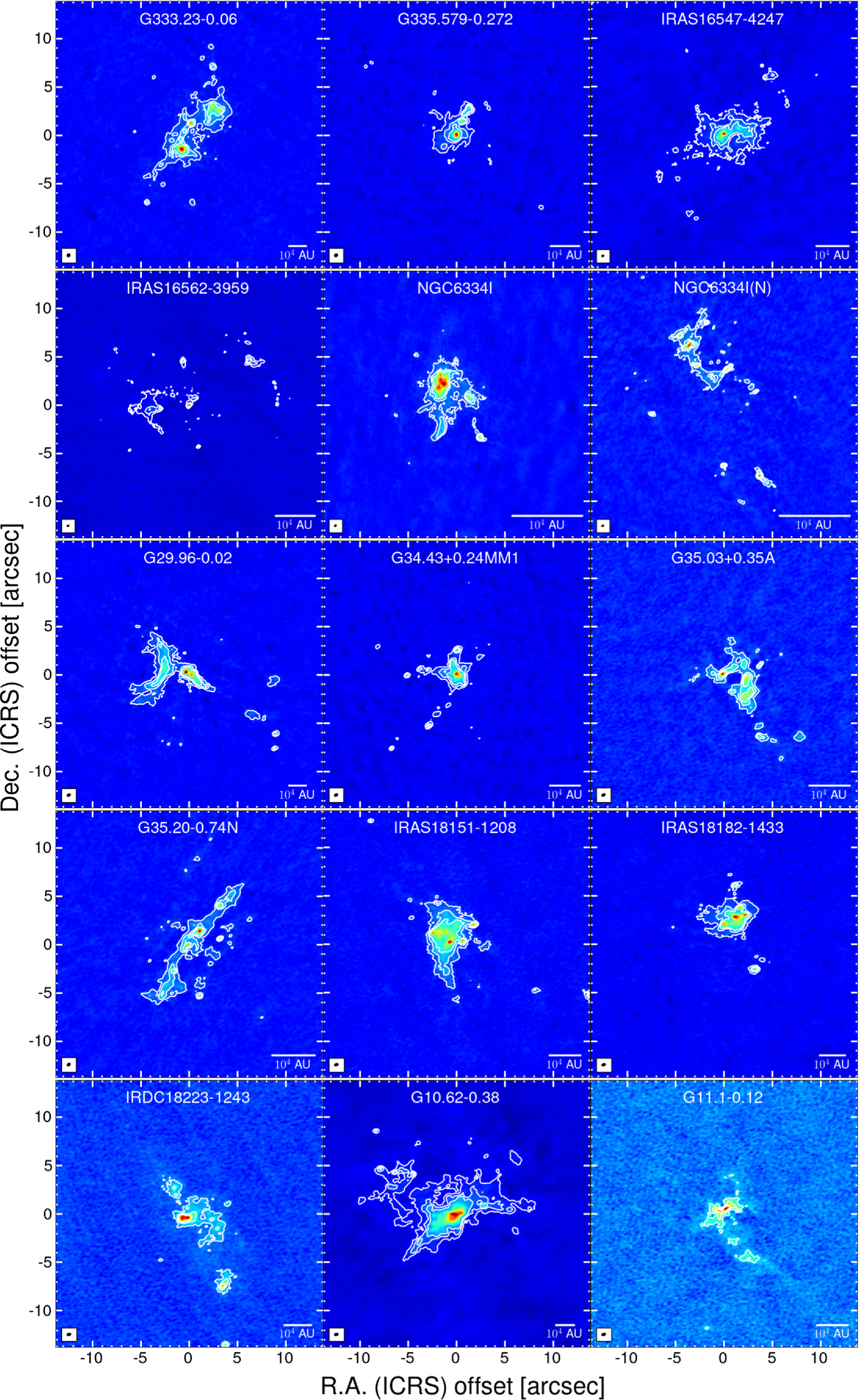
Figure 3 show the ALMA 1.33 mm dust continuum images of all targets. The internal structure of all the observed high-mass star-forming regions is well resolved and presents a variety of morphologies. Some of the DIHCA targets have emission highly concentrated near the clump center (e.g., IRAS 16547–4247, NGC 6334I, and G351.77-0.54), while in others the emission is relatively widespread (e.g., IRAS 16562–3959, G11.92-0.61, and G333.46-0.16). Some clumps present linearly aligned compact structures, resembling a fragmenting filament (e.g., G333.23-0.06, NGC 6334I(N), and G35.03 +0.35A).
Download figure:
Standard image High-resolution image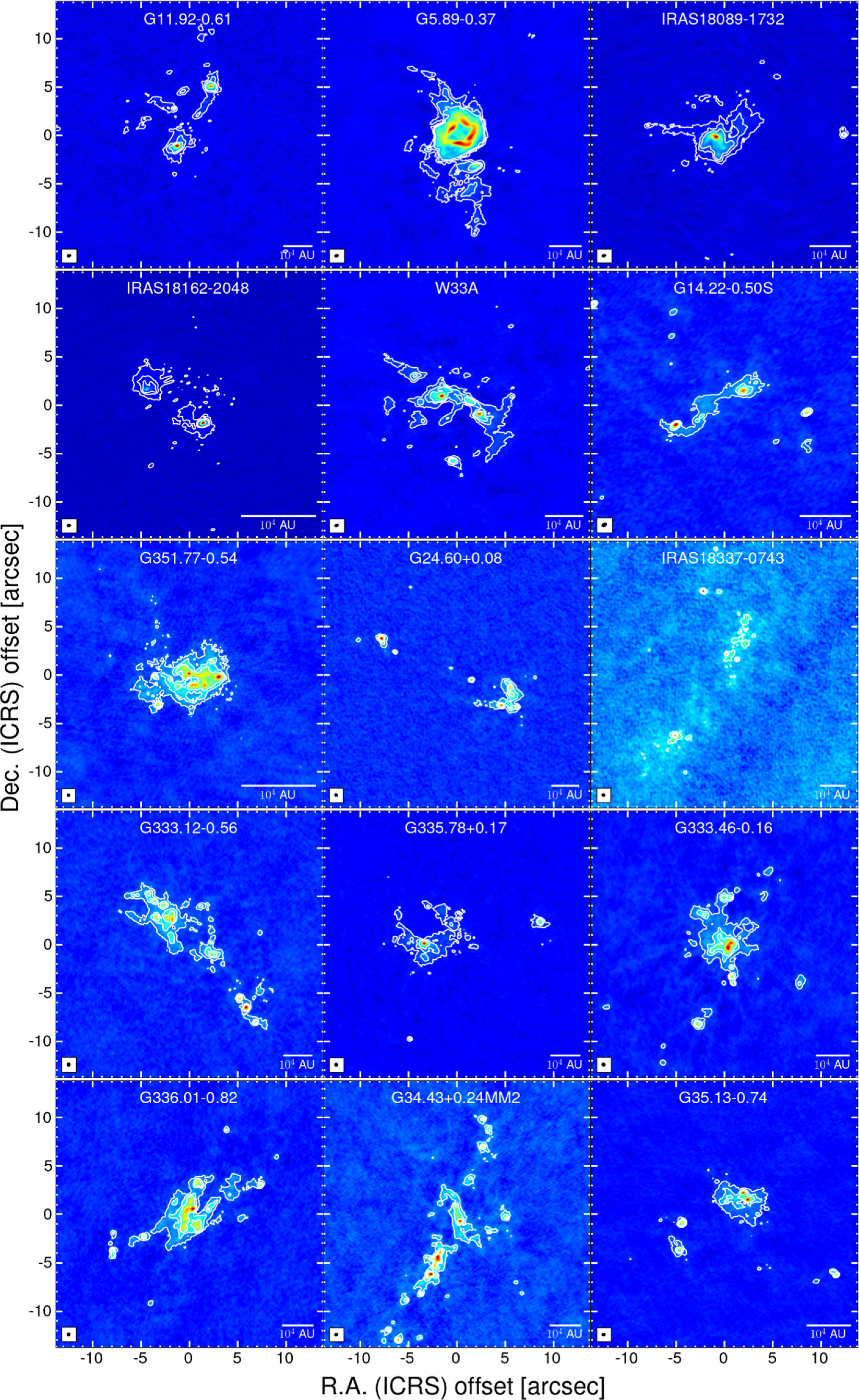
Figure 3. The overview of 1.33 mm continuum images for our targets on the same angular scale. The contour levels are [5, 15, 30] ×σ, with σ from column (2) in Table 2. The synthesized beam and scalebar are shown in the bottom-left and -right in each panel, respectively. The full views of each image with a color bar are shown in Appendix D.
Download figure:
Standard image High-resolution imageIndividual figures on each region can be found in Appendix D. The ALMA observations reveal that each clump has several compact structures, known as cores. Below, we describe how we uniformly identify these cores, as well as how we derive their physical properties.
4.2. Core Identification
We adopted the astrodendro package (Rosolowsky et al. 2008), which uses a dendrogram algorithm to compute hierarchical structures. We applied astrodendro to the continuum data without primary-beam correction, and identified the cores to measure their properties (integrated flux, peak flux, core size, and position). The astrodendro identifies three structures: leaf, branch, and trunk. We define the minimum structure, “a leaf,” as a core. The input parameters for dendrogram are three: min_value ( ), min_delta (
 ), and min_npix (
 ).
).
For min_value, we set  to remove nonreliable sources (σ is the rms noise written in Table 2). For min_delta, which helps to distinguish cores from neighboring structures, we adopt
  . The minimum pixel number, min_npix, was selected to be the corresponding number of pixels contained in a synthesized beam. After core identification, core fluxes were corrected by the primary-beam response. We identified 579 leaves in total and removed six leaves located at the edge of the primary beam with less than 30% response.
Table 3 lists the peak flux, integrated flux, position, and size of cores obtained from the dendrogram. The identified cores are labeled in ascending order from 1 in descending order of the peak flux of the core. The final number of identified cores (hereafter  ) used for analysis is 573. On average, each clump contains 19 cores. The number of identified cores
  varies from region to region ranging from 5 to 38 (see Table 5 for each clump). The wide range of
  may be attributed to the differences in clump properties, the noise level (or mass sensitivity), and the linear resolutions. A summary of core physical properties per clump is presented in Table 5.
Table 3. Core Properties as Dendrogram Output
| Clump | Core | Position (ICRS) | Peak | Integrated | FWHMmajor | FWHMminor | Radius | |
|---|---|---|---|---|---|---|---|---|
| Name | Name | R.A. (J2000) | Decl. (J2000) | flux | flux | |||
| (h:m:s) | (d:m:s) | (mJy beam−1) | (mJy) | (″) | (″) | (″) | ||
| G11.1-0.12 | ALMA1 | 18:10:28.25 | −19:22:30.37 | 6.56 | 8.50 | 0.46 | 0.20 | 0.15 |
| G11.1-0.12 | ALMA2 | 18:10:28.30 | −19:22:30.62 | 3.59 | 3.28 | 0.36 | 0.14 | 0.11 |
| G11.1-0.12 | ALMA3 | 18:10:28.09 | −19:22:35.17 | 0.93 | 2.69 | 0.75 | 0.35 | 0.26 |
| G11.1-0.12 | ALMA4 | 18:10:28.06 | −19:22:35.67 | 0.88 | 0.93 | 0.32 | 0.21 | 0.13 |
| G11.1-0.12 | ALMA5 | 18:10:28.19 | −19:22:33.77 | 0.72 | 1.90 | 0.61 | 0.37 | 0.24 |
Note.
Only a portion of this table is shown here to demonstrate its form and content. A machine-readable version of the full table is available.
Download table as: Machine-readable (MRT)Typeset image
In Figure 4, the top columns show  as a function of distance, rms noise level, and mass sensitivity. We also present the number of identified cores,
  , within the same physical area in the bottom columns. In this case, the total number of cores is calculated inside the circular area centered at the phase center of the observation whose diameter is the minimum FWHM among all observed targets (∼25″∼0.16 pc at 1.3 kpc). These figures indicate that the identified number of cores does not depend on the target distance, but the core number within the same physical area strongly depends on the distance. The dependencies of
  on rms noise level and mass sensitivity are weak.
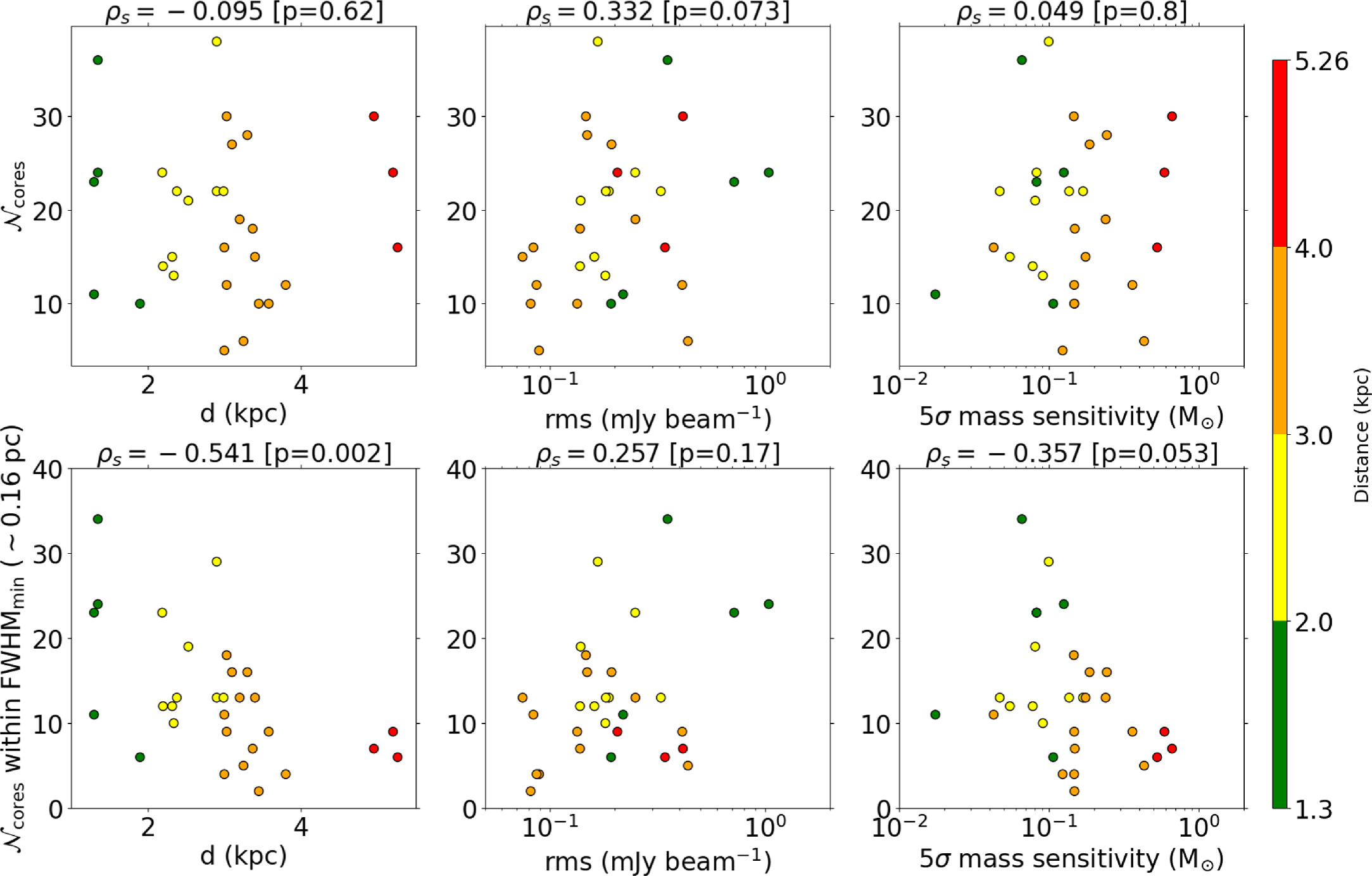
Figure 4. Top panels: target distance, rms noise level, and 5σ mass sensitivity against the number of identified cores. Bottom panels: target distances, rms noise level, and 5σ mass sensitivity against the number of identified cores within the same physical area whose diameter is the minimum of the FWHM (∼16 pc) of the FoV in the regions. The header of each panel shows the Spearman’s rank coefficient ρs and the p-value. The color coding shows the target distances.
Download figure:
Standard image High-resolution imageMore quantitatively, we applied Spearman’s rank correlation test. The test provides the Spearman’s rank correlation coefficient (ρs
) which is a measure to estimate the strength of the correlation between two variables for the classical and nonparametric test. Nonparametric tests are valid for small sample sizes and do not have to assume any distribution of the variables such as population distribution to be Gaussian. The value of ρs
is between −1 and 1. The closer ρs
is to +1 or −1, the stronger the positive or negative correlation, respectively. A value of 0 means no correlation. The derived values of ρs
are shown at the top of each panel of Figure 4. Each correlation with  is weak, with ∣ρs
∣ ≲ 0.3 (Figure 4, top panels). However, there are no statistically significant correlations because the probability value p > 0.05 for each test, corresponding to the probability that the correlation is a false relationship. On the other hand, the correlation between
is weak, with ∣ρs
∣ ≲ 0.3 (Figure 4, top panels). However, there are no statistically significant correlations because the probability value p > 0.05 for each test, corresponding to the probability that the correlation is a false relationship. On the other hand, the correlation between  within 0.16 pc and distance is strong, with ∣ρs
∣ ≳ 0.5 and p ≪ 0.05 (Figure 4, bottom panels). This is because the closer the target clumps, the higher the spatial resolution (∝d) and the mass sensitivity (∝d2).
within 0.16 pc and distance is strong, with ∣ρs
∣ ≳ 0.5 and p ≪ 0.05 (Figure 4, bottom panels). This is because the closer the target clumps, the higher the spatial resolution (∝d) and the mass sensitivity (∝d2).
4.3. Core Properties
By using the outputs from astrodendro analysis, we defined the physical quantities of each core. The position of each core is defined as the position of the pixel having the peak flux. The mass ( ) is calculated with Equation (4), assuming that the core temperature is the same as that of the parent clump. The surface density, column density, and volume density are estimated, respectively, using Equations (6), (7), and (8), replacing Mcl and Rcl by
  and
and  , respectively. The core radius (
 ) was defined as half of the geometric mean of the FWHMmajor and FWHMminor provided by astrodendro
13
(that is,
) was defined as half of the geometric mean of the FWHMmajor and FWHMminor provided by astrodendro
13
(that is,  ). The calculated physical quantities of all the identified cores are listed in Table 4, and Table 5 as the average values for each clump.
Table 4. Calculated Physical Properties of Identified Cores
| Clump | Core | Position (ICRS) |

|

| nave(H2) | Σave(H2) | Npeak(H2) | |
|---|---|---|---|---|---|---|---|---|
| Name | ID | R.A. (h:m:s) | Decl. (d:m:s) | (M⊙) | (au) | (×108cm−3) | (g cm−2) | (×1023cm−2) |
| G11.1-0.12 | ALMA1 | 18:10:28.25 | −19:22:30.37 | 2.36 | 450 | 7.71 | 32.59 | 32.20 |
| G11.1-0.12 | ALMA2 | 18:10:28.30 | −19:22:30.62 | 0.91 | 340 | 6.89 | 22.04 | 17.61 |
| G11.1-0.12 | ALMA3 | 18:10:28.09 | −19:22:35.17 | 0.75 | 770 | 0.50 | 3.57 | 4.55 |
| G11.1-0.12 | ALMA4 | 18:10:28.06 | −19:22:35.67 | 0.26 | 380 | 1.39 | 4.97 | 4.35 |
| G11.1-0.12 | ALMA5 | 18:10:28.19 | −19:22:33.77 | 0.53 | 710 | 0.44 | 2.94 | 3.52 |
Note.
Only a portion of this table is shown here to demonstrate its form and content. A machine-readable version of the full table is available.
Download table as: Machine-readable (MRT)Typeset image
Table 5. Core Average Properties Per Clump
| Source | 1σ Mass |

|

|

| Mean | ||||||
|---|---|---|---|---|---|---|---|---|---|---|---|
| Clump | Sensitivity | Min | Max | Median | Min | Max | Median | Σave(H2) | Npeak(H2) |

| |
| (M⊙) | (M⊙) | (M⊙) | (M⊙) | (au) | (au) | (au) | (g cm−2) | (×1023 cm−2) | (×108 cm−3) | ||
| G333.23-0.06 | 0.118 | 24 | 0.72 | 132.0 | 2.7 | 559 | 1704 | 807 | 28.7 | 35.0 | 3.3 |
| G335.579-0.272 | 0.087 | 6 | 0.98 | 127.2 | 10.8 | 386 | 1143 | 730 | 90.5 | 155.8 | 11.8 |
| IRAS 16547–4247 | 0.020 | 38 | 0.12 | 68.8 | 0.4 | 222 | 1128 | 344 | 20.0 | 26.6 | 5.4 |
| IRAS 16562–3959 | 0.009 | 22 | 0.07 | 9.1 | 0.4 | 150 | 606 | 247 | 41.8 | 55.3 | 18.9 |
| NGC 6334I | 0.025 | 24 | 0.18 | 58.9 | 0.5 | 105 | 486 | 150 | 246.1 | 247.4 | 144.4 |
| NGC 6334I(N) | 0.013 | 36 | 0.12 | 29.3 | 0.4 | 82 | 521 | 134 | 104.0 | 168.2 | 72.4 |
| G29.96-0.02 | 0.106 | 16 | 0.91 | 44.6 | 3.9 | 596 | 1628 | 772 | 37.5 | 36.2 | 5.0 |
| G34.43 + 0.24MM1 | 0.072 | 12 | 0.75 | 107.3 | 2.1 | 346 | 953 | 486 | 60.1 | 82.8 | 10.9 |
| G35.03 + 0.35A | 0.011 | 15 | 0.10 | 5.2 | 0.4 | 262 | 890 | 430 | 9.1 | 12.7 | 1.9 |
| G35.20-0.74N | 0.017 | 24 | 0.13 | 9.5 | 0.6 | 270 | 658 | 385 | 16.1 | 23.8 | 4.0 |
| IRAS 18151–1208 | 0.009 | 16 | 0.08 | 8.3 | 0.4 | 322 | 1142 | 477 | 9.1 | 12.6 | 1.7 |
| IRAS 18182–1433 | 0.030 | 10 | 0.29 | 20.5 | 4.4 | 430 | 774 | 564 | 45.2 | 50.2 | 8.5 |
| IRDC 18223–1243 | 0.035 | 15 | 0.29 | 27.1 | 0.8 | 395 | 1539 | 581 | 10.5 | 14.6 | 1.6 |
| G10.62-0.38 | 0.133 | 30 | 1.15 | 807.3 | 4.7 | 574 | 2452 | 864 | 35.5 | 40.3 | 3.7 |
| G11.1-0.12 | 0.025 | 5 | 0.26 | 2.4 | 0.7 | 341 | 768 | 452 | 13.2 | 12.4 | 3.4 |
| G11.92-0.61 | 0.030 | 18 | 0.22 | 42.2 | 0.8 | 390 | 1691 | 617 | 11.2 | 28.6 | 1.5 |
| G5.89-0.37 | 0.034 | 22 | 0.28 | 74.7 | 2.3 | 364 | 1918 | 757 | 64.2 | 69.4 | 9.5 |
| IRAS 18089–1732 | 0.018 | 13 | 0.16 | 64.7 | 0.4 | 298 | 1174 | 430 | 21.2 | 44.4 | 3.9 |
| IRAS 18162–2048 | 0.003 | 11 | 0.02 | 7.9 | 0.0 | 144 | 1042 | 220 | 25.1 | 63.6 | 9.0 |
| W33A | 0.016 | 21 | 0.17 | 14.6 | 1.1 | 312 | 1218 | 666 | 12.5 | 22.2 | 2.0 |
| G14.22-0.50S | 0.021 | 10 | 0.26 | 6.3 | 0.9 | 261 | 862 | 481 | 20.0 | 30.6 | 4.7 |
| G351.77-0.54 | 0.017 | 23 | 0.16 | 9.1 | 1.2 | 130 | 353 | 217 | 104.1 | 112.7 | 49.1 |
| G24.60 + 0.08 | 0.030 | 10 | 0.37 | 11.3 | 1.8 | 377 | 852 | 496 | 24.2 | 32.3 | 5.0 |
| IRAS 18337–0743 | 0.030 | 12 | 0.19 | 4.6 | 0.6 | 410 | 1189 | 540 | 6.6 | 8.8 | 1.2 |
| G333.12-0.56 | 0.049 | 28 | 0.33 | 28.6 | 1.7 | 419 | 1367 | 642 | 19.2 | 25.3 | 3.0 |
| G335.78 + 0.17 | 0.048 | 19 | 0.39 | 44.6 | 1.5 | 407 | 1347 | 687 | 19.0 | 37.0 | 2.8 |
| G333.46-0.16 | 0.027 | 22 | 0.20 | 35.0 | 0.8 | 322 | 1468 | 535 | 12.4 | 17.2 | 2.2 |
| G336.01-0.82 | 0.037 | 27 | 0.22 | 15.6 | 1.6 | 350 | 1047 | 558 | 21.9 | 23.4 | 4.4 |
| G34.43 + 0.24MM2 | 0.029 | 30 | 0.23 | 11.5 | 1.5 | 331 | 943 | 582 | 17.9 | 23.5 | 3.5 |
| G35.13-0.74 | 0.016 | 14 | 0.11 | 6.2 | 0.7 | 241 | 693 | 340 | 32.7 | 42.6 | 9.6 |
Note.
 ,
,  ,
,  , Σave(H2), Npeak(H2), and
  correspond to the number of cores, core mass, core radius, core average values of mean surface density, peak column density, and mean volume density.
Download table as: ASCIITypeset image
Figure 5 shows the relationship between the radius and mass of all identified cores color-coded by the distance with the plotted lines of constant column densities between 10−1 and 103 g cm−2, including the theoretical threshold of 1 g cm−2 suggested by Krumholz & McKee (2008) as the minimum surface density necessary for the formation of high-mass stars. Almost all cores satisfy this threshold. The mean surface density range is mostly distributed between ∼1 and 100 g cm−2 and some of the most massive cores have ≥100 g cm−2. There is a clear trend between radius and distance due to the broad distance range. The cores identified in clumps with the closest distances, ≲2 kpc, have somewhat higher column densities than those of cores in other clumps (see Table 1).
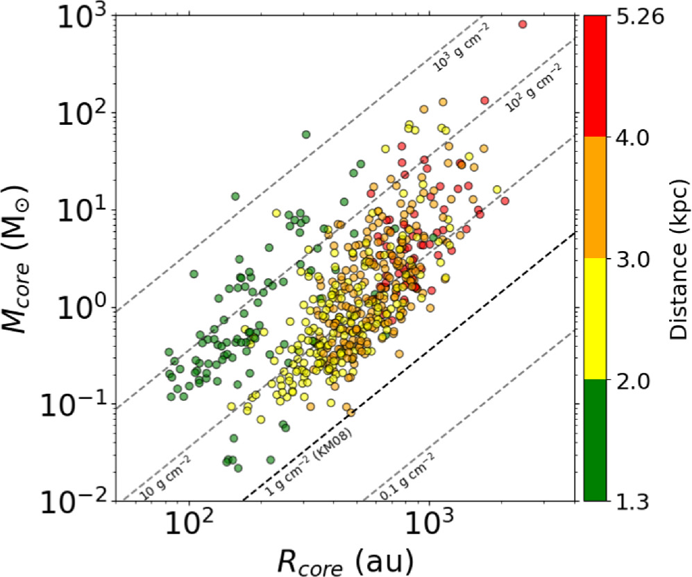
Figure 5. Masses vs. radius for all identified cores. Each dotted line represents a constant column density. The dashed line labeled KM08 represents the theoretical threshold of 1 g cm−1 suggested by Krumholz & McKee (2008), which corresponds to the column density ∼2.1 × 1023 cm−2. The color coding shows the target distances.
Download figure:
Standard image High-resolution imageNote that several clumps contain hot cores or H ii region (e.g., IRAS 18162–2048 and G5.89-0.37) and there is a discrepancy between clump and core average temperatures. This leads to an overestimation of the core mass and density, especially in the hot cores with the highest temperatures. Indeed, Taniguchi et al. (2023) found 44 hot cores using the CH3CN line. The derived excitation temperatures, which can represent the gas and dust temperature of the hot cores under LTE conditions, are larger than 70 K (see also Table 3 in Taniguchi et al. 2023).
In the current work, we mostly focus on the core separation and leave a more detailed analysis including the core mass once temperatures at high resolution are better constrained for the larger sample. For the moment we note that the distribution of core masses is comparable to the estimated thermal Jeans mass of the clumps, which is a result consistent with the subsequent discussion on thermal Jeans length.
4.4. Core Separations
The separation of the identified cores is most likely to reflect the fragmentation process. To measure the separations between cores, we applied the geometric algorithm, Minimum Spanning Tree (MST; Gower & Ross 1969) to the identified cores. This is one of the geometrical algorithms in graph theory. The connection of graph vertices with no closed loops is called a spanning tree so that given n vertices, a spanning tree has n − 1 edges. In the case of fragmentation analysis, vertices and edges correspond to core positions and separations, respectively. This analysis has been validated to detect multiple length scales of hierarchical structures (e.g., Clarke et al. 2019). The separation between the nearest neighboring cores, the length of an edge, is regarded as that produced by the fragmentation from the parental structure, following previous studies (e.g., Beuther et al. 2018; Sanhueza et al. 2019; Lu et al. 2020; Zhang et al. 2021; Morii et al. 2024). Here, we used the peak position of each core.
In Figure 6, we show the results of the MST analysis for W33A with a distance of 2.5 kpc, as an example. In this clump, the edges of MST appear to follow the cloud structure relatively well. For W33A, we identified 21 cores whose masses range from 0.17 to 14.6 M⊙ with a mean of 2.5 M⊙. In this area, a significant number of cores appears to be distributed along the elongated structure running from northeast to southwest, in which most massive cores reside. The core separations derived from MST range from 1130 to 19800 au with a mean of 4840 au. The mean value is about 6 times larger than the beam size of 830 au. The results from the MST analysis for other clumps are displayed in Appendix D.
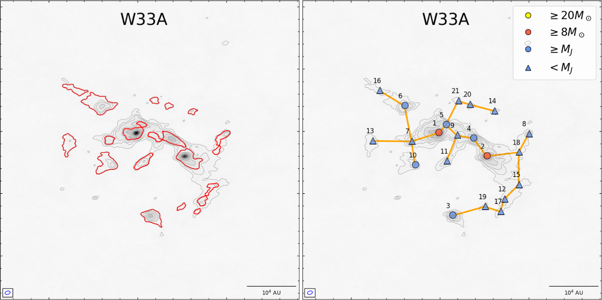
Figure 6. Left: core spatial distribution with red contours identified as leaves by dendrogram. The background shows the 1.33 mm continuum image with the contour levels at [5, 10, 15, 30, 60, 90] ×σ. Right: the left figure represents core mass and is overlaid with the result of MST. The number is ordered by the peak intensity. The orange edges are regarded as core separations for the spatial distribution.
Download figure:
Standard image High-resolution imageFigure 7 shows the separation distribution and the cumulative ratio for the whole DIHCA sample. The peaks of angular and physical separation are ∼148 and ∼4500 au, respectively, which is defined by the position at the maximum value of the logarithm probability density function (log-pdf) with a Gaussian Kernel (python module gaussian_kde in SciPy).
14
In angular scale, the peak of the separation distribution is ∼5 times the average angular resolution, ∼0
3 (Figure 7 top panel). The cumulative distribution of the core separations normalized to the beam size is presented in the middle panel of Figure 7. A total of 80% of core separations are resolved by more than three beams. If we separate the sample by distance, there are no clear differences in the distribution.
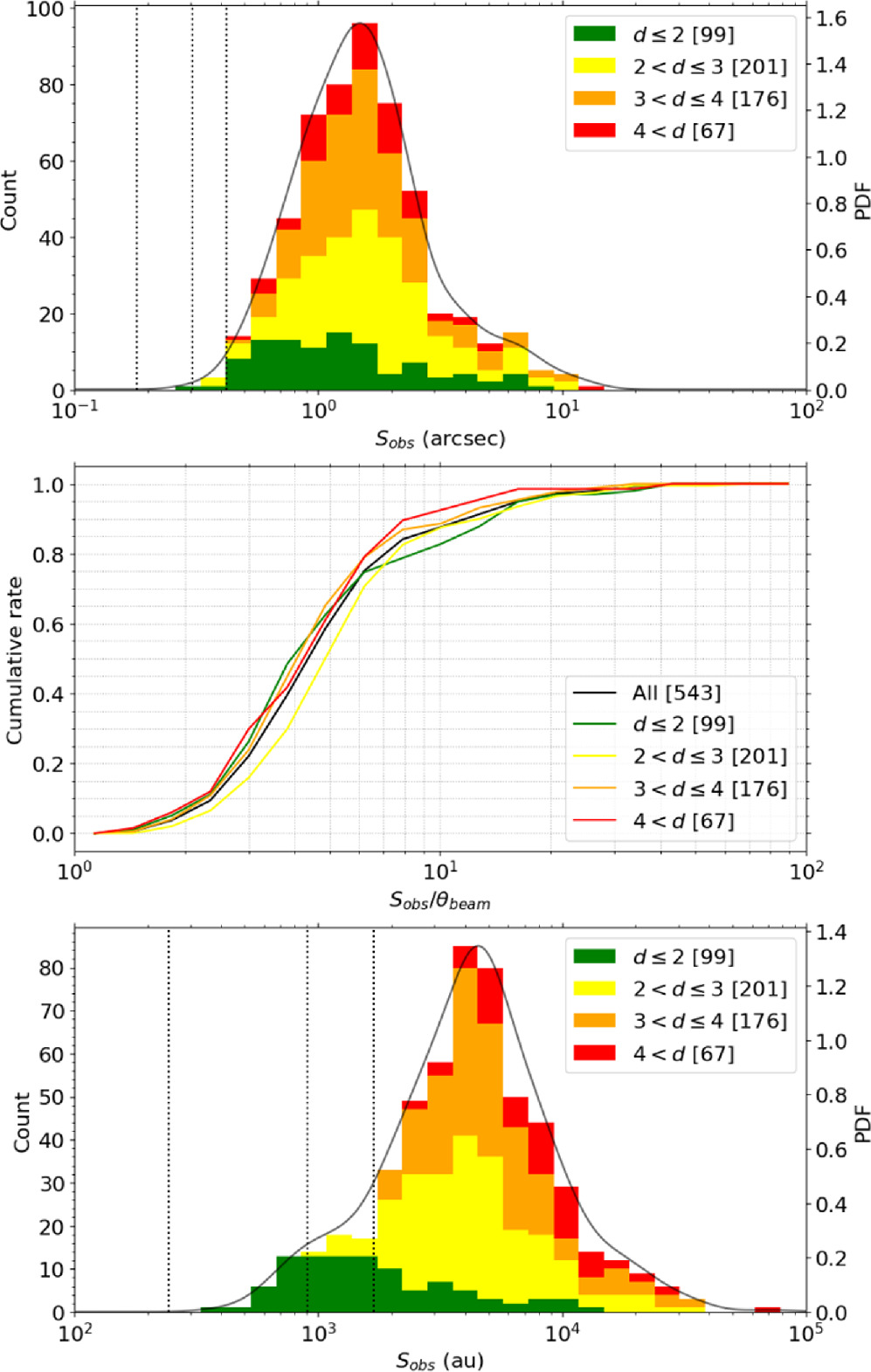
Figure 7. Top: distribution of the angular separation obtained from MST for the entire sample. The solid line shows the log-pdf produced by Gaussian Kernel Density Estimation. Vertical lines represent minimum, mean, and maximum angular resolutions, respectively. Middle: cumulative distribution of core separations divided by the angular resolution of the observations for clumps in each distance. Bottom: separation distribution in au scale by converting the angular separation into a physical separation using the source distance. Vertical lines represent minimum, mean, and maximum linear resolutions, respectively.
Download figure:
Standard image High-resolution imageIn physical scale and not yet considering projection effects (Figure 7 bottom panel), the separation distribution seems to have a peak at ∼4500 au with a shoulder at around 103 au and a tail at ≳104 au.
The core separation distribution appears to depend on the spatial resolution. Once the core distribution is classified into four groups with different distances: d < 2 kpc (green histogram), 2–3 kpc (yellow), 3–4 kpc (orange), and 4–5 kpc (red), we find that the shoulder at 103 au comes from the targets with the closest distance (<2 kpc) and the tail at larger separation is mostly explained by the more distant clumps (≥2 kpc). We will discuss the effect of spatial resolution in more detail in Section 5. The statistics of measured separations of each region are listed in Table 6.
Table 6. Derived Jeans Parameter and Measured Separations of Each Region
| Source |

|

| S3D (Original) | S3D (Smoothed) | ||||||
|---|---|---|---|---|---|---|---|---|---|---|
| Clump | Min | Max | Median | Mean | Min | Max | Median | Mean | ||
| (M⊙) | (au) | (au) | (au) | (au) | (au) | (au) | (au) | (au) | (au) | |
| G333.23-0.06 | 1.1 | 8100 | 3300 | 91,600 | 7800 | 13,300 | ⋯ | ⋯ | ⋯ | ⋯ |
| G335.579-0.272 | 1.1 | 7500 | 6200 | 47,900 | 7200 | 15,500 | 6200 | 9600 | 7200 | 7400 |
| IRAS 16547–4247 | 1.2 | 6500 | 1300 | 13,500 | 3500 | 4400 | 4300 | 20,500 | 10,600 | 10,200 |
| IRAS 16562–3959 | 3.6 | 13,300 | 1500 | 38,700 | 8900 | 12,200 | 5800 | 20,900 | 10,900 | 11,600 |
| NGC 6334I | 0.5 | 2500 | 500 | 5500 | 1500 | 2100 | 5600 | 7300 | 7000 | 6600 |
| NGC 6334I(N) | 0.5 | 3400 | 600 | 14,000 | 1500 | 3000 | 3200 | 14,400 | 5600 | 6800 |
| G29.96-0.02 | 2.6 | 11,300 | 4300 | 89,400 | 12,200 | 18,500 | ⋯ | ⋯ | ⋯ | ⋯ |
| G34.43 + 0.24MM1 | 0.8 | 5400 | 3000 | 17,200 | 6000 | 8800 | 2900 | 17,300 | 9600 | 9700 |
| G35.03 + 0.35A | 2.0 | 9800 | 2800 | 8000 | 5000 | 5000 | 3000 | 10,000 | 7500 | 6800 |
| G35.20-0.74N | 1.7 | 8900 | 2400 | 33,700 | 4100 | 5700 | 3200 | 14,300 | 6100 | 6200 |
| IRAS 18151–1208 | 2.7 | 12,100 | 3200 | 41,500 | 6900 | 11,600 | 3200 | 50,900 | 6800 | 12,700 |
| IRAS 18182–1433 | 1.5 | 9400 | 3500 | 20,700 | 5800 | 7500 | 3500 | 20,700 | 5800 | 7500 |
| IRDC 18223–1243 | 0.8 | 10,000 | 2300 | 26,200 | 5200 | 7800 | 2800 | 26,200 | 5200 | 8200 |
| G10.62-0.38 | 1.1 | 5600 | 3400 | 31,300 | 9800 | 10,900 | ⋯ | ⋯ | ⋯ | ⋯ |
| G11.1-0.12 | 1.4 | 13,400 | 2700 | 13,400 | 5100 | 6600 | 2700 | 13,400 | 10,400 | 9200 |
| G11.92-0.61 | 2.0 | 13,800 | 4000 | 30,700 | 7700 | 9100 | 4000 | 30,700 | 9300 | 10,400 |
| G5.89-0.37 | 1.3 | 6000 | 3200 | 12,600 | 6000 | 6800 | 3700 | 14,200 | 7100 | 7700 |
| IRAS 18089–1732 | 1.0 | 6700 | 3300 | 27,300 | 7100 | 9100 | 3300 | 27,100 | 9900 | 11,500 |
| IRAS 18162–2048 | 1.9 | 7200 | 900 | 8700 | 1600 | 3000 | 6200 | 11,200 | 8700 | 8700 |
| W33A | 1.3 | 8200 | 2800 | 10,200 | 6400 | 6300 | 3500 | 12,400 | 7800 | 7900 |
| G14.22-0.50S | 0.8 | 8200 | 3900 | 20,000 | 9300 | 10,200 | 2300 | 24,700 | 13,800 | 13,900 |
| G351.77-0.54 | 0.5 | 2400 | 800 | 3100 | 2000 | 2000 | 11,300 | 11,300 | 11,300 | 11,300 |
| G24.60 + 0.08 | 1.3 | 12,600 | 2600 | 36,900 | 8800 | 10,400 | 2600 | 36,800 | 8800 | 10,400 |
| IRAS 18337–0743 | 1.8 | 14,100 | 2900 | 45,200 | 7300 | 12,000 | 2900 | 45,200 | 7300 | 12,000 |
| G333.12-0.56 | 0.7 | 7000 | 3000 | 20,200 | 5700 | 6700 | 3000 | 20,200 | 5800 | 6800 |
| G335.78 + 0.17 | 1.3 | 8500 | 2500 | 35,200 | 5600 | 9300 | 2600 | 35,100 | 5600 | 9300 |
| G333.46-0.16 | 1.3 | 8000 | 2500 | 26,100 | 7200 | 9300 | 3800 | 30,200 | 9000 | 10,900 |
| G336.01-0.82 | 0.8 | 6000 | 2600 | 25,700 | 6400 | 7400 | 3000 | 26,800 | 6900 | 8100 |
| G34.43 + 0.24MM2 | 1.2 | 9100 | 2700 | 14,000 | 4900 | 5900 | 3100 | 14,000 | 6200 | 6800 |
| G35.13-0.74 | 1.0 | 8000 | 1400 | 25,200 | 3700 | 6200 | 5400 | 33,500 | 11,700 | 15,600 |
Note. Thermal Jeans Mass is derived as  .
.
Download table as: ASCIITypeset image
5. Discussion
5.1. Characteristic Fragmentation Scale
5.1.1. Core Separation Normalized to the Clump Jeans Length
We compare the core separations measured with MST to a characteristic length scale, the clump thermal Jeans length ( ). The clump thermal Jeans lengths are calculated from the clump temperature and density listed in Table 1. The Jeans length ranges from 2000 and 14,000 au. The derived values are listed in Table 6.
We show the core separation distribution normalized to the clump Jeans length in Figure 8 (a). The left panel shows the core distribution corrected for projection effects, while the right panel is that normalized to the clump thermal Jeans length. The projection effect on the actual 3D separation distribution has been discussed in Sanhueza et al. (2019) and Li et al. (2021), for example. Assuming that the observed cores have a spherically uniform distribution, a correction factor of 4/π is applied to the projected distance Sobs. This is based on the probability density of the solid angle between core separation and the line-of-sight direction. Thus, the deprojected separation S3D is estimated as follows;
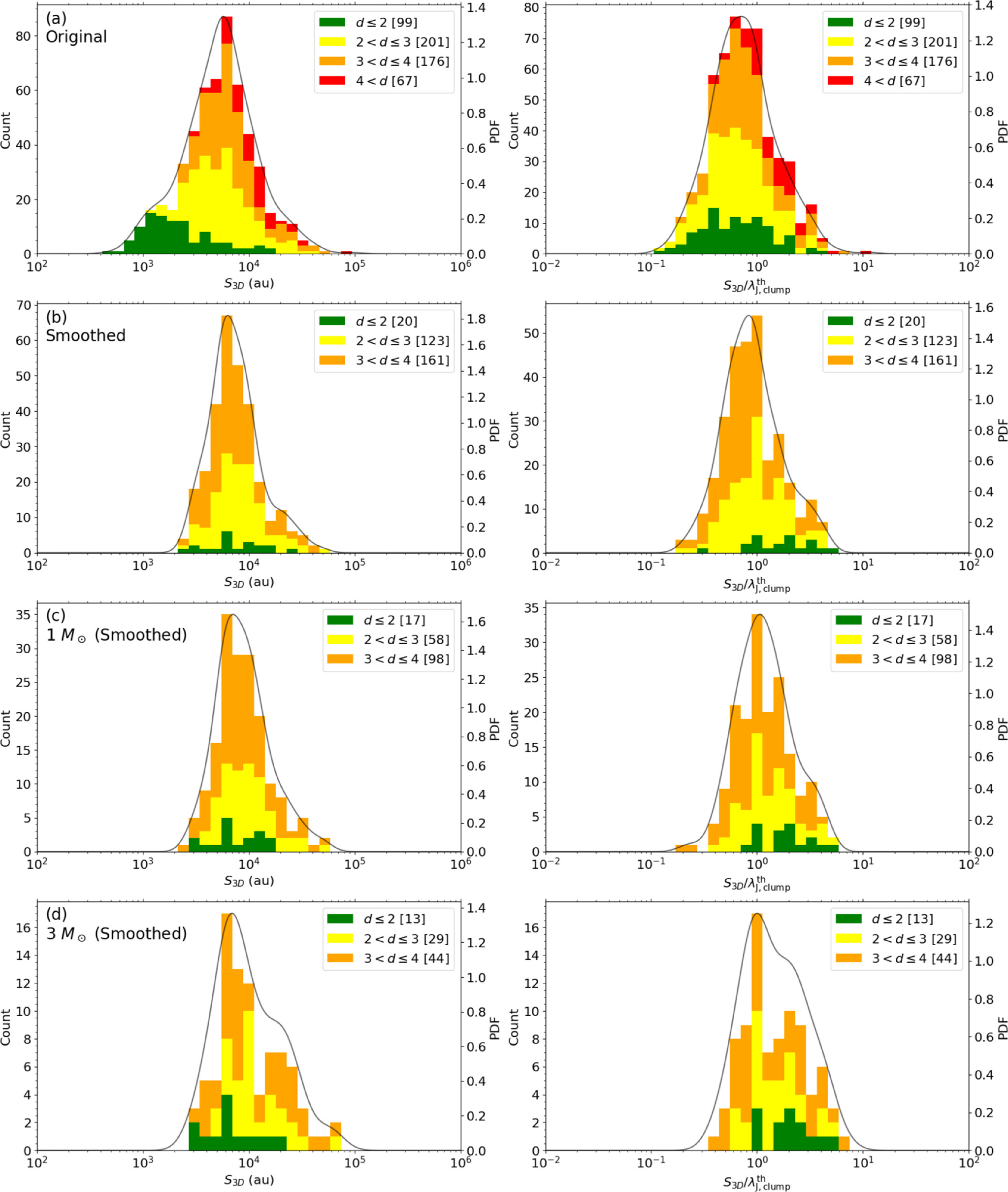
Figure 8. Separation distribution in various styles. Left panels display them on a physical scale. Right panels display them in normalized to the clump thermal Jeans length. Each column is represented as follows. Core separation is measured from (a) original images, (b) smoothed images, (c) for cores whose mass is higher than 1 M⊙, and (d) the cores whose mass is higher than 3 M⊙.
Download figure:
Standard image High-resolution imageThe peak of the separation distribution corrected by projection effects is ∼5800 au. The normalized separation appears to have a single peak at  with no clear shoulder due to close star-forming regions. The tail at large values also becomes more subtle. The clumps with the closest distances have larger clump densities, and thus the Jeans lengths tend to be smaller. The impact of varying the core identification parameters on the core separation distribution is discussed in Appendix A.
Beuther et al. (2018) observed 20 high-mass star-forming clumps with similar properties to those in the DIHCA sample at a similar angular resolution with NOEMA. They identified 123 cores using clumpfind, finding a 3D core separation distribution with a peak at around 2500 au. To make a direct comparison with their work, we have reanalyzed their images and identified 129 cores using dendrograms under the same parameters we used in the DIHCA sample. The newly derived separation distribution, corrected by projection effects, has a peak at ∼5600 au, consistent with the value derived in the DIHCA sample. The reason why the difference occurred despite a similar number of cores is mainly due to different core identification methods. Despite similar parameter settings with dendrogram, clumpfind tends to identify compact and sharp sources. Thus, separation distribution by clumpfind is distributed on a smaller scale than that of dendrogram.
5.1.2. The Effects of Different Spatial Resolution
As mentioned in Section 4.4, the separation distribution may be affected by the spatial resolution. Because the spatial resolution is proportional to the distance of the target under a similar beam size (∼03 in this work), the broad distance range of the clumps tends to make the separation distribution more flattened. We minimize the effect of having different spatial resolutions in the core separation analysis by smoothing the continuum images. We used the CASA task imsmooth and smoothed the dust continuum images to the angular resolution equivalent to ∼1100 au. We decided to exclude three clumps that are more distant than 4 kpc (corresponding to a spatial resolution of ≳1600 au) to keep the spatial resolution range as small as possible after smoothing. We identified the cores in the smoothed images and made the separation distribution of cores using the MST analysis with the same procedure applied in the original images (Section 4.2). As a result, the total number of identified cores is reduced from 573 in the 30 clumps to 331 in 27 clumps. Figure 8 (b) shows the separation distribution between cores obtained from the smoothed images. The separation distribution is similar to the original. The peak separation is about 6300 au and 0.84
 , (∼8%) larger than the values obtained from the original images.
Similarly as done in Figure 4, we check for a correlation between the number of cores from the smoothed images with observational quantities. Figure 9 shows the correlations between distance, rms noise, and mass sensitivity. For both the total number of cores and the number of cores within 0.08 pc, there is a weak or no correlation with each quantity.
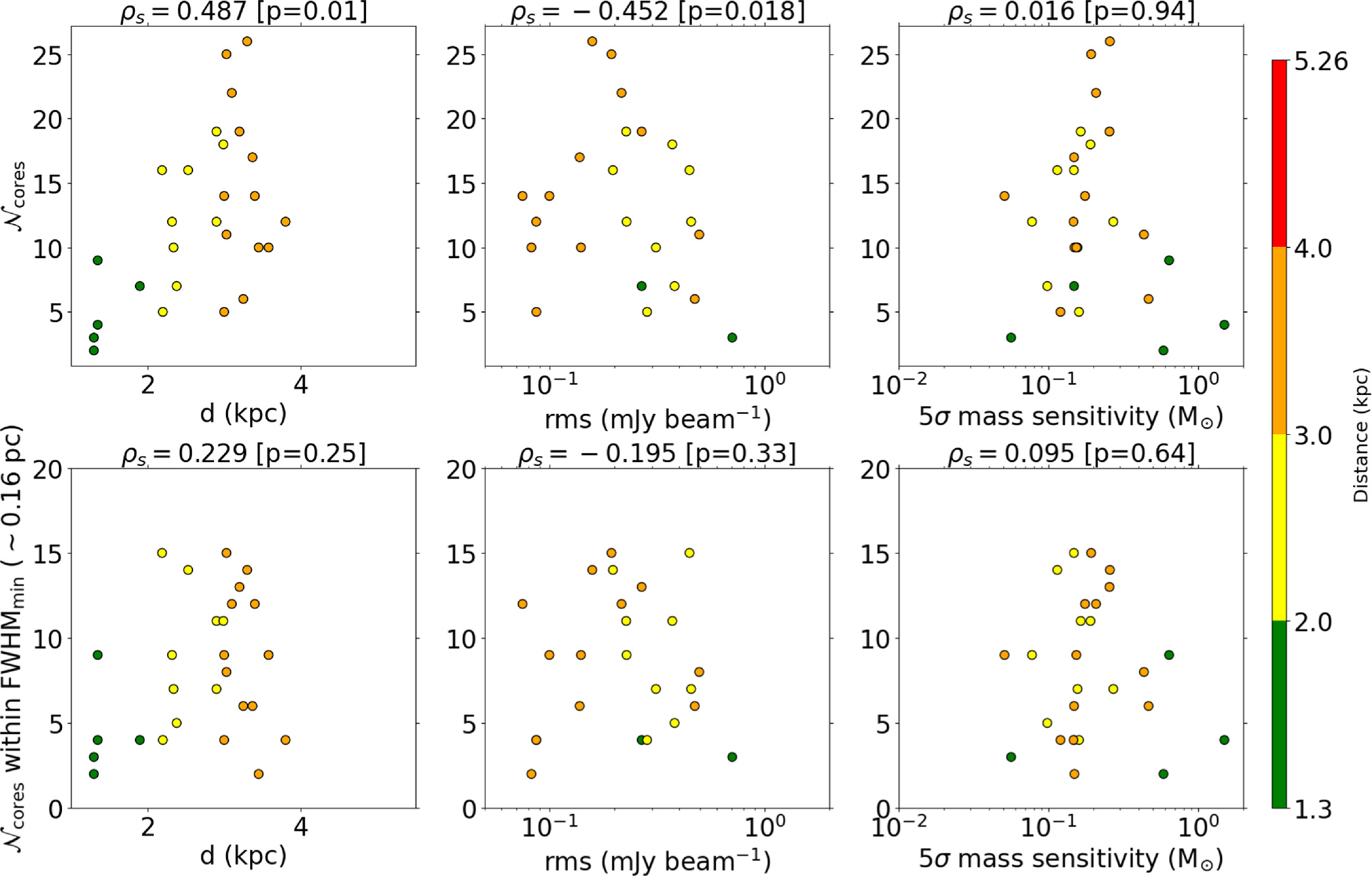
Figure 9. Same as Figure 4 except for the sample from smoothed images.
Download figure:
Standard image High-resolution image5.1.3. The Effects of Completeness
To compute the mass completeness limit, we insert a circular, beam size, flat core in each image per trial. The positions of the artificial cores are determined with a uniform probability in the field of view. Then, we applied a dendrogram to identify cores. We repeated this simulation 2000 times. Sometimes, the inserted core overlaps and merges with an existing core. In such a case, the core is counted as one detection. Figure 10 shows the completeness analysis for a given mass. The core detection rate increases with increasing core mass. For most of the clumps, the detection rate shows a similar dependence on the core mass. In a few regions, the morphology of the continuum emission affects the actual detection rate. For example, the detection rate of NGC 6334I has a bump at around 0.4 M⊙. The clump looks centrally condensed, and the overlap of the inserted cores may somewhat reduce the detection rate. The G10.62-0.38 region shows the poorest mass completeness since it is one of the most distant clumps in our sample (d = 4.95 kpc). However, the detection rate reaches more than 90% by 3 M⊙ for all the clumps, except for three targets that have the worst mass sensitivity (G333.23-0.06, G29.96-0.02, and G10.62-0.38, which correspond to the three clumps located at distances larger than 4 kpc).
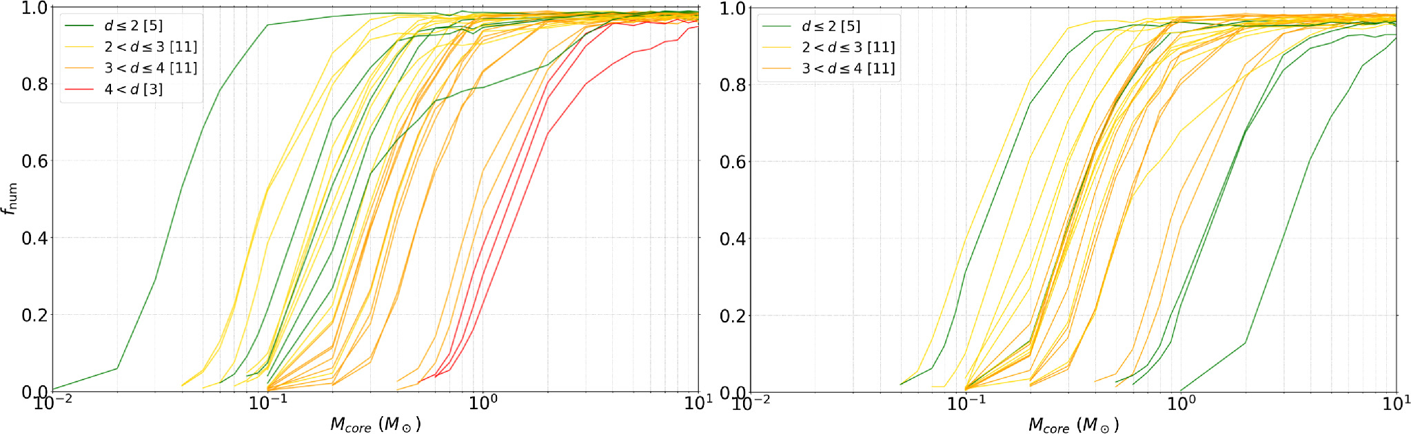
Figure 10. The mass detection rate of each region for original (left) and smoothed (right) images. The three clumps whose distance is ≥4 kpc are excluded (see Section 5.1.2). The color coding is the same as the previous figures.
Download figure:
Standard image High-resolution imageTo explore the effect of having different mass sensitivities, we set the minimum mass for the smoothed images as  1 M⊙ and 3 M⊙ and applied the MST to measure the core separations. For
  M⊙ and 3 M⊙, the core separation peaked at 7200 au and 7100 au, respectively (see also Figure 8 (c), (d)). Figure 11 summarizes the dependence of the core separation on the minimum core mass. The marker and error bar illustrate the peak position and the dispersion of the separation distribution. The higher the mass restriction, the smaller the sample size, and the larger the dispersion of the separation distribution. Except for no restriction case, all of the peak positions are within the margin of error and the peak separation appears not to be sensitive to the minimum core mass. Thus, we conclude that the core separation peaks at around 7000 au, irrespective of the observational bias such as the different angular resolution and mass sensitivity. The peak values of each separation distribution defined by different mass limits, as shown in Figure 11, are listed in Table C1.
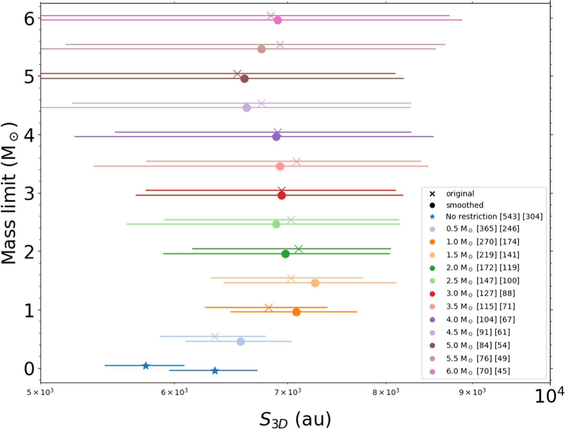
Figure 11. The peak positions of the probability density function (pdf) for each separation distribution in which core identification was restricted by the core mass. The error bar represents the dispersion of the separation distribution. To avoid the duplication of error bars, the y locations are slightly shifted from actual values. For the square brackets in the legend, the left and right values of each marker display the total sample of MST from original images and smoothed images, respectively.
Download figure:
Standard image High-resolution image5.2. Characteristic Fragmentation Scale in High-mass Star-forming Clumps
In Section 5.1, we concluded that the peak separation is comparable to the thermal Jeans length of the clumps and there is no need to invoke turbulent Jeans fragmentation. However, numerical simulations on cluster formation suggest that a number of density structures are created by diverse physical processes, e.g., fragmentation, merging, accretion, and turbulence, and such structure formation proceeds hierarchically (e.g., Klessen & Burkert 2000; Bate 2012; Myers et al. 2013; Federrath 2015; Wu et al. 2017; Hennebelle & Inutsuka 2019; Vázquez-Semadeni et al. 2019). Local turbulence tends to compress and form elongated denser substructures, such as filaments and sheets. Within these denser regions, which have weaker turbulence, fragmentation into cores is expected to take place. Filaments and sheets can also be generated as a result of anisotropic gravitational contraction (e.g., Burkert & Hartmann 2004; Heitsch et al. 2009; Gómez & Vázquez-Semadeni 2014). Then, protostars (or sink particles) created by fragmentation can gain additional mass from the surroundings so that their final stellar masses are determined (Bate 2019; Pelkonen et al. 2021). Here, we consider such a case in which the turbulent clumps create hierarchical structures during their global contraction, forming sheets or filaments as substructures from which dense cores are formed by gravitational fragmentation.
Below, we compare the clump thermal Jeans length with the characteristic fragmentation scale of the filaments and sheets. For simplicity, we first consider an isothermal axisymmetric cylindrical cloud in dynamical equilibrium. The equilibrium solution was derived by Stodólkiewicz (1963). According to this work, the cloud radius can be expressed as
where ρcyl is the density of the cylinder. The fragmentation wavelength of this cylindrical cloud has been obtained by several authors (e.g., Larson 1985; Inutsuka & Miyama 1992). Stodólkiewicz (1963) obtained the critical wavelength above which the perturbation grows in time. The wavelength of the maximum linear growth rate is about twice the critical wavelength, which is about 8 times longer than the cylinder radius.

If the cylinder density is f times higher than the clump density, ρcyl = f ρcl, the fragmentation scale of the cylinder can be expressed as

For an isothermal sheet, the thickness of the equilibrium sheet (Spitzer 1978) can be given as

The fragmentation scale for the equilibrium sheet (e.g., Larson 1985) can be estimated as

where ρsh = f ρcl.
Numerical simulations of cluster formation show that the densities of substructures created by either local turbulent compression or anisotropic gravitational contraction are about ≳10 times higher, that is, f ≳ 10 (e.g., Klessen & Burkert 2000; Bate 2012, 2019; Myers et al. 2013; Wu et al. 2017; Hennebelle & Inutsuka 2019; Pelkonen et al. 2021). We also estimate the average density from our ALMA data to roughly evaluate f. Here, we consider that the structures identified as trunks
15
are the direct precursors of filaments and sheets. We then derive the average density (ρtrunk) as the total trunk mass divided by the trunk volume for each target. We calculate the volume of a trunk assuming a spherical symmetry with a radius of  , excluding trunks that have no substructures (leaves). For all the cases, the trunks having hierarchical structures reside near the center of the FoV. The ratio between the trunk radius and the Maximum Recoverable scale ranges between 0.09 and 1.08, with about 90% of the values smaller than 1. This means that for some trunks, the determined density is a lower limit. The values of f = ρcl/ρtrunk are estimated to be several tens with a mean value of f ≃ 40 and a median value of f ≃ 27. Therefore, considering that for some trunks the density is a lower limit, we conclude that f ∼ 10 is a reasonable estimation.
In such a case, the fragmentation scale of either a cylinder or a sheet is almost equal to the clump thermal Jeans length (within 13%),  . This analysis indicates that our peak separation is consistent with both clump thermal Jeans length and the fragmentation scale of a dense cylinder or sheet. However, it is worth noting that if the fragmentation scale is primarily determined by filament fragmentation, the filament width should be about 7000 au/ 4 = 1750 au (≃8.5 × 10⁻³ pc), which is about 10 times smaller than that of the proposed constant filament width (≈0.1 pc) model (André et al. 2014). This implies that filament fragmentation is not a dominant process to create dense cores, or that the filament width is not universal and is significantly smaller than those of nearby star-forming regions. In reality, recent several observations found filaments with small widths in Orion A (e.g., Hacar et al. 2018; Monsch et al. 2018; Suri et al. 2019; Teng & Hirano 2020) and Perseus (e.g., Schmiedeke et al. 2021; Chen et al. 2022). At the average clump density of 106 cm−3, the Jeans length is 5600 au or 0.027 pc, and in the central denser parts of the clumps, it is much smaller. Therefore, the Jeans length in the clumps, thus the core separation, is likely to be much shorter than that predicted by fragmentation of the 0.1 pc universal width filaments (André et al. 2014). These might indicate that the filament width is unlikely to be universal in high-mass star-forming clumps.
5.3. Comparison with Previous Studies
We compare our results with those of similar previous studies targeting high-mass star-forming regions. The comparative studies are the following three surveys: CORE/20 clumps (Beuther et al. 2018), SQUALO/13 clumps (Traficante et al. 2023), and ASHES/12 clumps (Sanhueza et al. 2019). Our sample is referred to as DIHCA. ASHES is a mosaic observation covering ∼1 arcmin2, while the others are single-pointing observations. For CORE, we show the reanalyzed result by astrodendro (see Section 5.1.1).
Figure 12 shows a box plot of the clump luminosity-to-mass ratio (Lbol/Mclump) for each survey. In the ASHES survey, they selected 70 μm-dark objects, representing the earliest evolutionary stage among the samples to be compared. On the other hand, In the CORE sample, luminous objects with >104 L⊙ were selected, making it the most evolved sample. In SQUALO and DIHCA samples, no thresholds were considered in the luminosity or Lbol/Mclump parameter, and include objects at various evolutionary stages. Figure 13 plots the mass-size relationship of the clumps, indicating that the density of ASHES targets is ∼104–105 cm−3, lower than the targets in the other surveys.
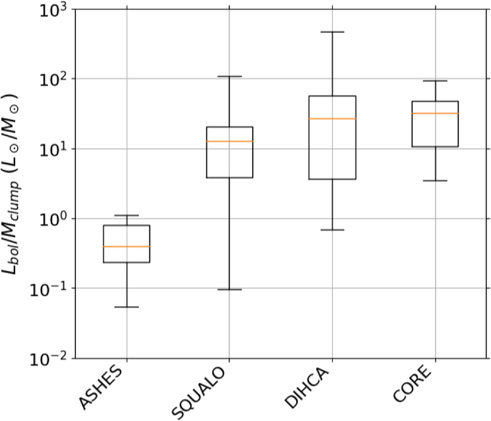
Figure 12. The box plot of clump luminosity-to-mass ratio (Lbol/Mclump) for each survey.
Download figure:
Standard image High-resolution image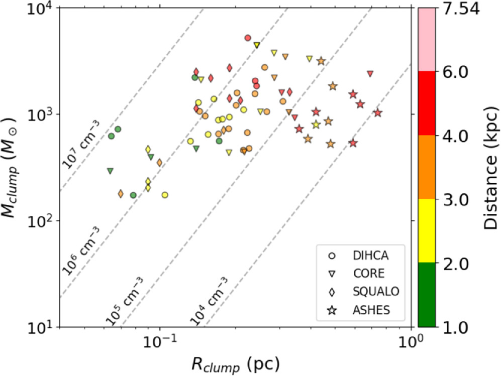
Figure 13. Clump mass against radius including other surveys. The dashed lines represent the corresponding average volume density assuming spherical symmetry. The color coding shows the target distance.
Download figure:
Standard image High-resolution imageThe upper panel of Figure 14 plots the relationship between the 1σ mass sensitivity and spatial resolution for each survey. DIHCA and CORE have spatial resolutions up to ∼2000 au, while SQUALO and ASHES have resolutions of ∼2000–8000 au. The mass sensitivity of SQUALO is ≳0.1 M⊙, while the others have ≲0.1 M⊙. The lower panel plots the ratio of the estimated thermal Jeans mass to the 1σ mass sensitivity and the ratio of the thermal Jeans length to the spatial resolution. This also shows that SQUALO can only resolve the thermal Jeans mass by ≲10 and the thermal Jeans length by ≲3, which is nearly an order of magnitude smaller than the other surveys. Our tests in Sections 5.1.2 and 5.1.3 showed that the separation distributions of the nearby clumps (green histograms) in Figure 15 differ significantly between (a) original and (b), (c), (d) smoothed, suggesting that the effects of insufficient resolution and mass sensitivity are reflected. It is highly likely that a similar phenomenon is occurring in the separation distribution of SQUALO. Thus, we do not seek a physical meaning in the separation distribution of SQUALO. For the calculation of thermal Jeans mass and thermal Jeans length in each survey, we used the mass, radius, and temperature from Table 1 of Sanhueza et al. (2019) for ASHES, and from Table 3 of Traficante et al. (2023) for SQUALO. For CORE, we estimated the mass and radius using the same method as ours toward SCUBA 850 μm data of 17 clumps. Although the rotational temperature of H2CO emission lines has been estimated as gas kinetic temperature by Beuther et al. (2018), the temperature range is high at ∼40–160 K except for one region, which deviates from the clump temperatures of other surveys. Therefore, we assumed a temperature of 23.2 K, which is the median temperature of DIHCA clumps. Indeed, Izumi et al. (2024) find evidence that the H2CO kinetic temperature is not tracing ambient gas, but it is rather tracing the molecular outflows.
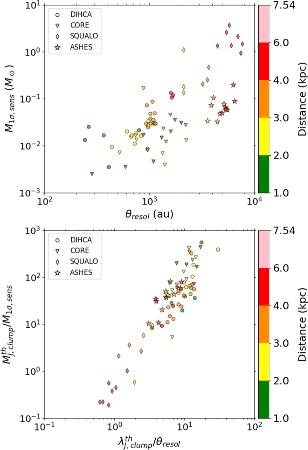
Figure 14. Top: relationship between 1σ mass sensitivities and spatial resolutions of each survey. Bottom: relationship between thermal Jeans mass divided by 1σ mass sensitivity ( ) and thermal Jeans length divided by spatial resolution (
 ) of each survey. The color coding shows the target distance.
Download figure:
Standard image High-resolution image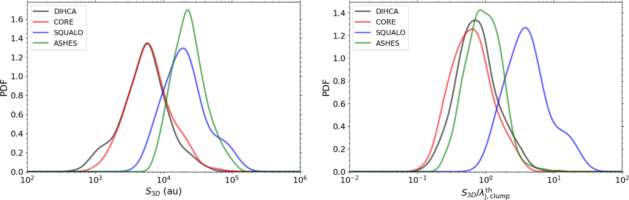
Figure 15. Separation distribution in physical scale (left) and in normalized to clump thermal Jeans length (right).
Download figure:
Standard image High-resolution imageFigure 15 shows the log-pdf of the separation distribution for each survey (same as Figure 10). Comparing the distribution of physical scales in the left panel, it is clear that the distributions of CORE and DIHCA are distinctly different from those of ASHES and SQUALO. These differences in distribution are thought to be mainly due to differences in spatial resolution and evolutionary stage. Spatial resolution determines the lower limit of resolvable separation and inevitably affects the separation distribution. Regarding the difference in the evolutionary stage, the effect of tighter separation due to gravity as evolution progresses may also be reflected (e.g., Traficante et al. 2023; Xu et al. 2024). Interestingly, the peak position of DIHCA and CORE is ∼6000 au. This value has also been found in previous studies such as Xu et al. (2024; ASSEMBLE survey), Tang et al. (2019; W51 North), Palau et al. (2018; OMC-1S), and Lu et al. (2020; CMZ), suggesting the existence of a universal fragmentation scale.
Looking at the distribution of scales normalized by the thermal Jeans length in the right panel of Figure 15, CORE, DIHCA, and ASHES are around ∼0.8. ASHES clumps are at an earlier evolutionary stage compared to CORE and DIHCA, but it shows a separation distribution that is similarly consistent with the thermal Jeans length. In this way, previous studies also show consistent results, robustly supporting the hypothesis that thermal Jeans fragmentation is dominant on a ≲1 pc scale.
This result is supported by other previous studies up to ∼1 pc scale that focus on aspects other than the fragmentation scale. Gutermuth et al. (2011) proposed a simple picture of the thermal fragmentation of high-density gas in an isothermal self-gravitating layer to explain the correlation between YSO surface density and gas column density they found in eight molecular clouds within 1 kpc. Palau et al. (2015) compared the “fragmentation level” with the Jeans mass and Jeans number of 19 massive dense cores with a size of ∼0.1 pc. They found that it shows a good correlation when thermally supported rather than turbulent supported. Thus, the overall results of this work along with the results of previous works seem to consistently support a scenario where thermal Jeans fragmentation is at work.
6. Summary
We have presented the core properties of 30 high-mass star-forming clumps obtained by the Digging into the Interior of Hot Cores with ALMA (DIHCA) survey, at a typical angular resolution of ∼03.
We have searched for dense cores using the 1.3 mm continuum emission maps and identified 579 cores in total using dendrograms. We have derived the separation between cores using the Minimum Spanning Tree (MST) technique and the obtained separation distribution that has a peak at ∼5800 au.
In order to remove possible observational biases produced by the variation of spatial resolution and sensitivity in the observed sample, we smoothed the data and ran completeness tests. We have concluded that the characteristic fragmentation scale of the observed high-mass star-forming regions, which are representative of the Galactic population, is ∼7000 au. This characteristic scale is comparable to the thermal Jeans length of the observed clumps.
Numerical simulations of the dense cores suggest that circumstellar disks tend to fragment to form binaries or multiple systems. In that case, the separation is likely to be <1000 au. In a few cases, we indeed observed short separations among cores, especially in the closest regions (d ≲ 2 kpc). Disk fragmentation is difficult to resolve from the present data used in this work, but it is possible with the extended configuration observations taken as part of the DIHCA survey. Disk fragmentation will be studied in detail in forthcoming works.
Acknowledgments
This work was supported in part by The Graduate University for Advanced Studies, SOKENDAI. P.S. was partially supported by a Grant-in-Aid for Scientific Research (KAKENHI Number JP22H01271 and JP23H01221) of JSPS. K.I. was supported by the ALMA Japan Research Grant of NAOJ ALMA Project, NAOJ-ALMA-329. This paper makes use of the following ALMA data: ADS/JAO.ALMA#2016.1.01036.S, ADS/JAO.ALMA#2017.1.00237.S. ALMA is a partnership of ESO (representing its member states), NSF (USA), and NINS (Japan), together with NRC (Canada), MOST and ASIAA (Taiwan), and KASI (Republic of Korea), in cooperation with the Republic of Chile. The Joint ALMA Observatory is operated by ESO, AUI/NRAO and NAOJ. Data analysis was in part carried out on the Multiwavelength Data Analysis System operated by the Astronomy Data Center (ADC), National Astronomical Observatory of Japan.
Facilities: ALMA - Atacama Large Millimeter Array, IRSA - , Spitzer - Spitzer Space Telescope satellite, APEX - Atacama Pathfinder Experiment, JCMT - James Clerk Maxwell Telescope.
Software: CASA (McMullin et al. 2007), astrodendro (Rosolowsky et al. 2008), Astropy (Price-Whelan et al. 2018), SciPy (Virtanen et al. 2020), Matplotlib (Hunter 2007).
Appendix A: The Effect of Core Identification Parameters
Here we confirm the impact toward separation distributions in the case of adopting the different core identification parameters (Section 4.2). We tested several cases changing the minimum intensity of the core  and the minimum step to distinguish the neighboring structures
  . The ranges of
  and
and  are between 5–7σ and 1–2σ with the step of 1σ, respectively.
Table A1 lists the numbers of identified cores, and peak positions in angular, physical, and normalized scales of each case. Figure A1 shows each separation distribution on a physical scale and normalized scale. The peak positions for different dendrogram parameters are shown in Figure A2. In both scales, we can find that the separation distributions are almost indistinguishable, mostly keeping the same shape and peak position, for different input dendrogram parameters. Thus, we concluded that the difference in dendrogram parameters has no large impact on peak positions and shape of separation distributions.
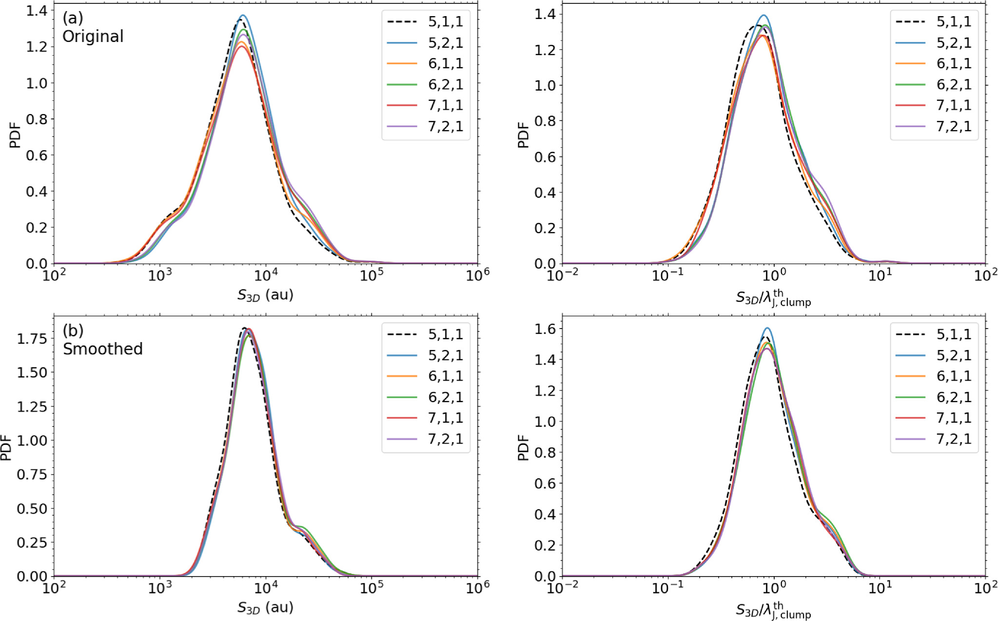
Figure A1. The probability density functions (pdf) of each separation distribution for different dendrogram parameters in physical scale (left) and normalized scale (right). Core separation was measured from (a) original images and (b) smoothed images, respectively.
Download figure:
Standard image High-resolution image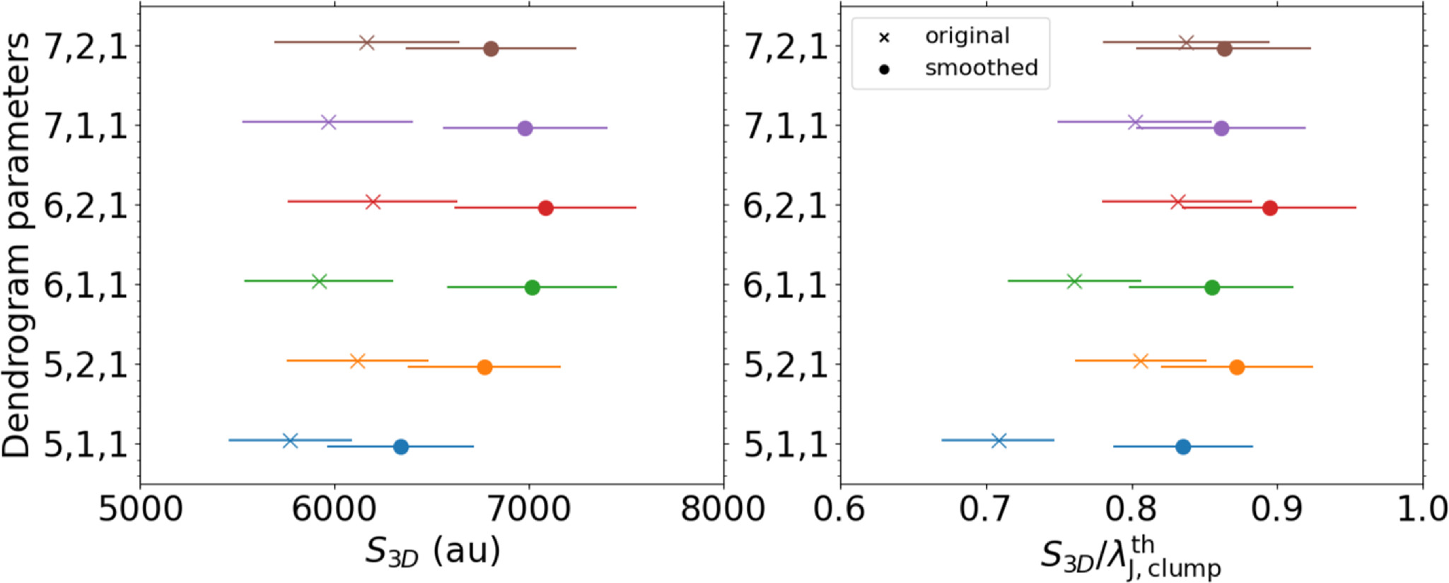
Figure A2. The peak positions of the probability density function (pdf) for each separation distribution whose core identification was restricted by the core mass. The error bar represents the dispersion of the separation distribution. To avoid the duplication of error bars, the y locations are slightly shifted from actual values. For the square brackets in the legend, the left and right values of each marker display the total sample of MST from original images and smoothed images, respectively.
Download figure:
Standard image High-resolution imageTable A1. Peak Values of Separation Distribution for Each Dendrogram Parameter
| Identification |

|

| ||
|---|---|---|---|---|
| Condition | (arcsecond) | (au) | ( ) ) | |
| Original | ||||
| (5,1,1) | 573 | 1.48 | 5800 | 0.71 |
| (5,2,1) | 486 | 1.63 | 6100 | 0.81 |
| (6,1,1) | 477 | 1.50 | 5900 | 0.76 |
| (6,2,1) | 420 | 1.58 | 6200 | 0.83 |
| (7,1,1) | 406 | 1.52 | 6000 | 0.8 |
| (7,2,1) | 374 | 1.61 | 6200 | 0.84 |
| Smoothed | ||||
| (5,1,1) | 331 | 1.67 | 6300 | 0.84 |
| (5,2,1) | 296 | 1.92 | 6800 | 0.87 |
| (6,1,1) | 274 | 1.88 | 7000 | 0.85 |
| (6,2,1) | 257 | 1.91 | 7100 | 0.89 |
| (7,1,1) | 242 | 1.83 | 7000 | 0.86 |
| (7,2,1) | 235 | 1.84 | 6800 | 0.86 |
Note. For the first column, the three numbers in parentheses represent the coefficients of  (×σ, left),
  (×σ, middle), and
  (×θbeam, where θbeam means the corresponding number of pixels contained in a synthesized beam right), respectively.
The peak value is defined by the position at the maximum value of the logarithm probability density function (log-pdf) with a Gaussian Kernel.
Download table as: ASCIITypeset image
Appendix B: The Effect of Evolutionary Processes
Here we confirm the impact toward separation distributions by evolutionary processes. Our analysis depends on the assumption that the fragmentation scale reflects on the core separations. However, in the more evolved clumps, the assumption can break because of the stellar feedback or dynamical process. Actually, G5.89-0.37 has a shell structure in the central region created by explosive events (Zapata et al. 2020; Fernández-López et al. 2021). The central shell is identified as four cores by the dendrogram. The separation distributions in such regions may not keep the fragmentation scale. To consider the effect, we derived the separation distribution without the most evolved 12 regions which are more likely to be affected by stellar feedback or dynamical process. The most evolved regions are selected based on the existence of extended 8 μm emission which means characteristic of the emission from photodissociation region produced mostly by polycyclic aromatic hydrocarbons emission. The selected 12 regions are IRAS 16562–3959, NGC 6334I, C35.20-0.74(N), G29.96-0.02, IRAS 18182–1433, G10.62-0.38, G5.89-0.38, IRAS 18162–2048, W33A, G351.77-0.54, G333.46-0.16, and G336.01-0.82.
Figure B1 shows each separation distribution. The black line and red line represent the separation distribution of all regions and the remaining 18 regions which excluded the most evolved 12 regions, respectively. We concluded that the effect of dynamical effect has no large impact on peak positions and the shape of separation distributions.
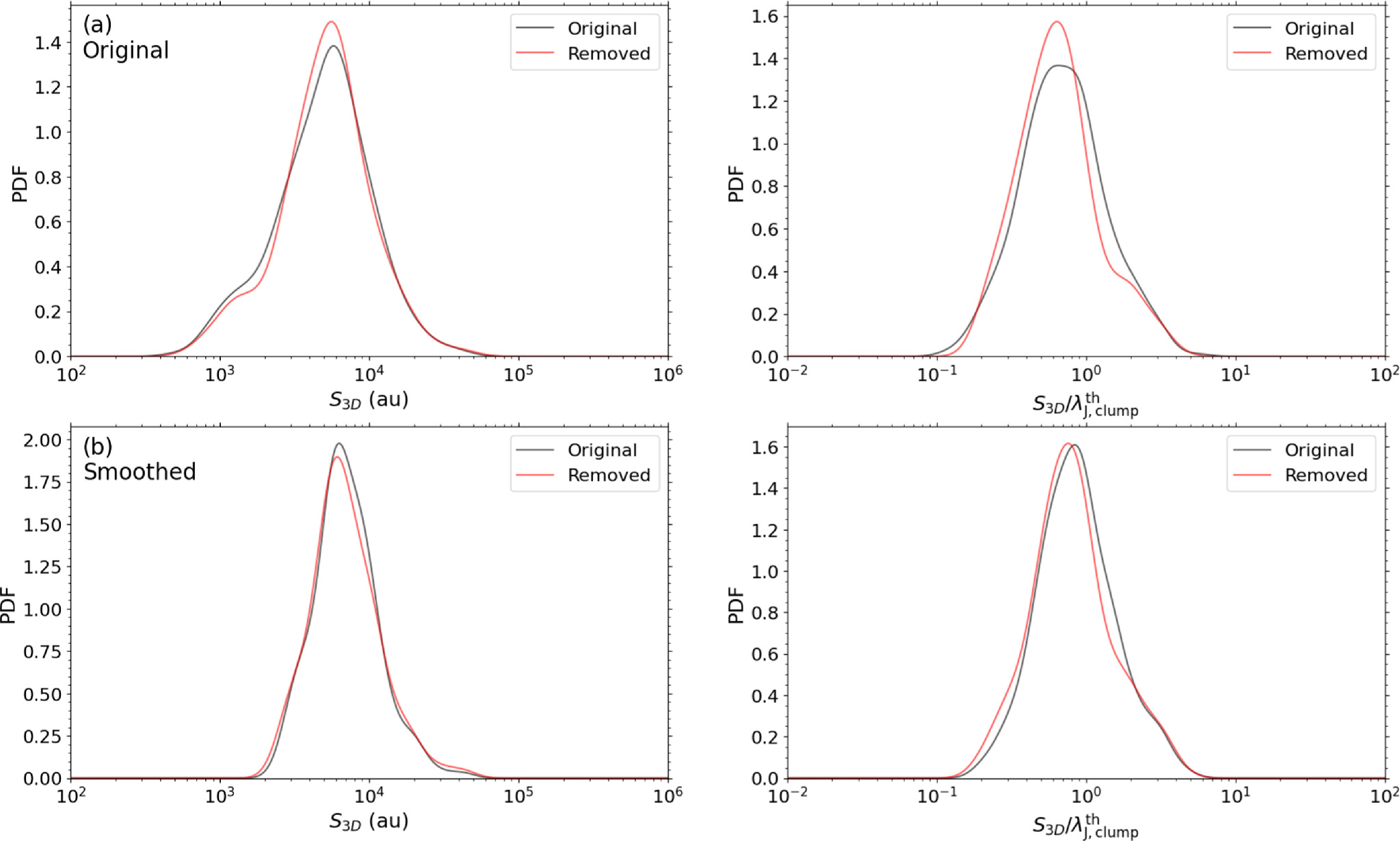
Figure B1. The probability density functions (pdf) of each separation distribution for different evolutionary stages in physical scale (left) and normalized scale (right). Core separation was measured from (a) original images and (b) smoothed images, respectively.
Download figure:
Standard image High-resolution imageAppendix C: Statistics of Separations
Here, Table C1 lists the sample number and peak separation of each mass restriction for core identification Original and Smoothed.
Table C1. Peak Values of Separation Distribution for Each Condition
| Identification |

|

| ||
|---|---|---|---|---|
| Condition | (arcsecond) | (au) | ( ) ) | |
| Original | ||||
| no restriction | 573 | 1.48 | 5800 | 0.71 |
| ≥ 0.5 M⊙ | 395 | 1.59 | 6300 | 0.87 |
| ≥ 1.0 M⊙ | 299 | 1.69 | 6800 | 0.94 |
| ≥ 1.5 M⊙ | 248 | 1.75 | 7000 | 1.02 |
| ≥ 2.0 M⊙ | 201 | 1.72 | 7100 | 0.97 |
| ≥ 2.5 M⊙ | 175 | 1.67 | 7000 | 0.94 |
| ≥ 3.0 M⊙ | 152 | 1.65 | 6900 | 0.92 |
| ≥ 3.5 M⊙ | 140 | 1.63 | 7100 | 0.97 |
| ≥ 4.0 M⊙ | 129 | 1.67 | 6900 | 0.96 |
| ≥ 4.5 M⊙ | 115 | 1.75 | 6800 | 0.94 |
| ≥ 5.0 M⊙ | 104 | 1.71 | 6500 | 0.93 |
| ≥ 5.5 M⊙ | 94 | 1.87 | 6900 | 0.99 |
| ≥ 6.0 M⊙ | 87 | 1.94 | 6800 | 1.77 |
| Smoothed | ||||
| no restriction | 331 | 1.67 | 6300 | 0.84 |
| ≥ 0.5 M⊙ | 273 | 1.8 | 6600 | 0.84 |
| ≥ 1.0 M⊙ | 200 | 1.95 | 7100 | 1.07 |
| ≥ 1.5 M⊙ | 167 | 2.12 | 7300 | 1.08 |
| ≥ 2.0 M⊙ | 145 | 1.93 | 7000 | 1.04 |
| ≥ 2.5 M⊙ | 126 | 1.9 | 6900 | 1.06 |
| ≥ 3.0 M⊙ | 113 | 1.87 | 6900 | 1.01 |
| ≥ 3.5 M⊙ | 96 | 1.95 | 6900 | 1.07 |
| ≥ 4.0 M⊙ | 92 | 1.89 | 6900 | 1.05 |
| ≥ 4.5 M⊙ | 83 | 1.82 | 6600 | 0.99 |
| ≥ 5.0 M⊙ | 72 | 1.8 | 6600 | 1.01 |
| ≥ 5.5 M⊙ | 66 | 1.75 | 6800 | 1.03 |
| ≥ 6.0 M⊙ | 62 | 1.75 | 6900 | 1.02 |
Note. The peak value is defined by the position at the maximum value of the logarithm probability density function (log-pdf) with a Gaussian Kernel.
Download table as: ASCIITypeset image
Appendix D: The Individual Targets
Here we illustrate clump scale single-dish images composed of submillimeter continuum data and infrared data. In addition, the results of dendrogram analysis and MST analysis are also presented. Figure D1 shows an example of G333.23-0.06.
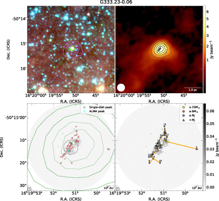
Figure D1. Top left: large-scale overview images of Spitzer/IRAC 3.6, 4.5, and 8.0 μm images overlaid ATLASGAL 870 μm dust continuum emission contours. The contour levels for the ATLASGAL 870 μm continuum are [0.2, 0.4, 0.6, 0.8] ×peak flux, with peak flux =6.9 Jy beam−1. Top right: ATLASGAL 870 μm continuum colormap and the contour same as top left. In addition, ALMA 1.33 mm continuum contours are plotted internal white dotted circle which represents a field of view for ALMA. The contour levels are [5, 10, 15, 30, 60, 90] ×σ, with σ = 0.206 mJy beam−1. Bottom left: ALMA 1.33 mm continuum gray-scale map and the red contours as the results of core identification by astrodendro. The green dashed contour shows the ATLASGAL 870 μm continuum same as the top panels. The green cross shows the peak position of ATLASGAL 870 μm continuum emission. The cyan cross shows that of ALMA 1.33 mm continuum emission. Bottom right: The result of core separation analysis by MST.
Download figure:
Standard image High-resolution imageFootnotes
- 10
NASA/IPAC Infrared Science Archive, https://sha.ipac.caltech.edu/applications/Spitzer/SHA/.
- 11
The ATLASGAL Database Server, https://atlasgal.mpifr-bonn.mpg.de/cgi-bin/ATLASGAL_DATABASE.cgi.
- 12
The JCMT Science Archive, https://www.cadc-ccda.hia-iha.nrc-cnrc.gc.ca/en/jcmt/.
- 13
Details can be seen in https://dendrograms.readthedocs.io/en/stable/.
- 14
- 15
See here for a visual explanation of the differences between leaves, branches, and trunks as defined in dendrograms: https://dendrograms.readthedocs.io/en/stable/.