Abstract
We characterize the chemical and physical conditions in an outflowing high-velocity cloud (HVC) in the inner Galaxy. We report a supersolar metallicity of [O/H] = +0.36 ± 0.12 for the HVC at vLSR = 125.6 km s−1 toward the star HD 156359 (l = 3287, b = −14
5, d = 9 kpc, z = −2.3 kpc). Using archival observations from the Far-Ultraviolet Spectroscopic Explorer (FUSE), the Hubble Space Telescope Imaging Spectrograph, and the European Southern Observatory Fiber-fed Extended Range Optical Spectrograph we measure high-velocity absorption in H i, O i, C ii, N ii, Si ii, Ca ii, Si iii, Fe iii, C iv, Si iv, N v, and O vi. We measure a low H i column density of log N(H i) = 15.54 ± 0.05 in the HVC from multiple unsaturated H i Lyman series lines in the FUSE data. We determine a low dust depletion level in the HVC from the relative strength of silicon, iron, and calcium absorption relative to oxygen, with [Si/O] = −0.33 ± 0.14, [Fe/O] = −0.30 ± 0.20, and [Ca/O] = −0.56 ± 0.16. Analysis of the high-ion absorption using collisional ionization models indicates that the hot plasma is multiphase, with the C iv and Si iv tracing 104.9 K gas and N v and O vi tracing 105.4 K gas. The cloud’s metallicity, dust content, kinematics, and close proximity to the disk are all consistent with a Galactic wind origin. As the HD 156359 line of sight probes the inner Galaxy, the HVC appears to be a young cloud caught in the act of being entrained in a multiphase Galactic outflow and driven out into the halo.
Original content from this work may be used under the terms of the Creative Commons Attribution 4.0 licence. Any further distribution of this work must maintain attribution to the author(s) and the title of the work, journal citation and DOI.
1. Introduction
The supermassive black hole, Sgr A*, and surrounding regions of active star formation power an outflowing multiphase wind from the center of the Milky Way (MW). Outflows play a critical role in the baryon cycle, the cycling of gas into and out of galaxies, which helps regulate the evolution of galaxies. The MW offers us a front-row seat view to study outflows over a range of wavelengths and phases and understand their impact on galaxy evolution.
Presently, the farthest-reaching known outflows in the MW are the Fermi (Su et al. 2010; Ackermann et al. 2014) and eROSITA (Bland-Hawthorn & Cohen 2003; Predehl et al. 2020) bubbles, which are giant gamma- and X-ray emission extending ∼10 kpc and 14 kpc above and below the Galactic disk, respectively (see Figure 1). The origin of the Fermi Bubbles is believed to be an energetic Galactic center (GC) Seyfert flare event ∼3.5 Myr ago (Bland-Hawthorn et al. 2019).
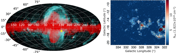
Figure 1. Left: the location of HD 156359 with reference to the Fermi and eROSITA bubbles. The composite FermieROSITA image from Predehl et al. (2020), where the softer X-ray emission (0.6–1 keV, in cyan) envelopes the harder component of the extended GeV emission of the Fermi bubbles (in red; adapted from Selig et al. 2015). Right: H i column-density map from the 21 cm HI4PI survey showing the distribution of H i in the region from 100 to 150 km s−1 (HI4PI Collaboration et al. 2016) in a section of “Complex WE” by Wakker & van Woerden (1991). The location of HD 156359 is marked with a white cross. The contours correspond to log NH i = 2.08, 6.23, 10.4, 14.5, 18.7 × 1018 cm−2.
Download figure:
Standard image High-resolution imageUltraviolet (UV) absorption-line studies have found gas outflowing at high velocity in a number of sight lines passing through or near the Fermi Bubbles (see Keeney et al. 2006; Zech et al. 2008; Fox et al. 2015; Bordoloi et al. 2017; Savage et al. 2017; Karim et al. 2018; Ashley et al. 2020, 2022). These high-velocity clouds (HVCs) consist of neutral (e.g., C i, O i), singly ionized (S ii, Si ii, Fe ii), and highly ionized (C iv, Si iv, O vi) gas. Cold gas has also been detected in the nuclear outflow via emission in neutral hydrogen and molecules. Several hundred H i 21 cm clouds have been detected at low latitudes in the Fermi Bubbles outflowing from the GC (McClure-Griffiths et al. 2013; Di Teodoro et al. 2018; Lockman et al. 2020). Carbon monoxide (CO) has been detected in submillimeter emission in two dense molecular clouds comoving within the H i 21 cm outflow (Di Teodoro et al. 2020). More recently, molecular hydrogen was discovered in the Galactic nuclear outflow ∼1 kpc below the GC (Cashman et al. 2021). Outflowing gas associated with the Fermi Bubbles has also been seen in optical emission (Krishnarao et al. 2020a). Together, these observations of HVCs near the GC provide observational constraints on the properties of the MW nuclear wind.
The outflowing wind interacts with gas in the disk in multiple ways. First, it can disrupt the position and velocity of the disk (Krishnarao et al. 2020b), leading to warps and perturbations. Second, it can accelerate and entrain cool gas into the halo. In some instances, this high-velocity gas may cool, lose buoyancy, and fall back onto the disk as a “Galactic fountain,” supplying new fuel for further star formation (see Shapiro & Field 1976; Bregman 1980; Kahn 1981; de Avillez 1999). In other cases, the high-velocity gas may survive being accelerated into the halo, and even escape. Cloud survival is the subject of recent theoretical work focusing on how cool gas clouds develop and grow in the hot wind (see Gronke & Oh 2020; Sparre et al. 2020).
The metallicities of HVCs are important to determine because they provide direct evidence for the origin of the clouds (Richter 2017; Ashley et al. 2022). For example, the low metallicities seen in Complex A (≈0.1 solar; Wakker 2004) and Complex C (≈0.15 solar; Wakker et al. 1999; Richter et al. 2001; Collins et al. 2003; Tripp et al. 2003; Sembach et al. 2004) are consistent with a halo origin, tracing infalling gas from sources such as the intergalactic medium or satellite dwarf galaxies. The Smith Cloud (also known as Complex GCP), on the other hand, is more metal-rich (≈0.5 solar) and is thought to trace gas originating in the outer Galactic disk (Lockman et al. 2008; Hill et al. 2009; Fox et al. 2016), although this interpretation assumes a constant HVC gas metallicity over time, and therefore neglects metal mixing (Heitsch et al. 2022).
Fully UV-based metallicities (with the metal and H i column densities measured along the same UV sight lines) are ideal to ensure that the metal absorption and hydrogen absorption are tracing the same gas, but they are rare because of the difficulty in isolating unsaturated high-velocity H i components in UV absorption. These high-velocity H i components are often saturated or blended, even for high-order Lyman series lines, thus there is only a narrow range of N(H i) values for which precise measurements are possible (French et al. 2021). Therefore HVC metallicities are frequently determined from a combination of a UV measurement along an infinitesimal sight line with a H i measurement made using a much larger 21 cm beam. However, this combination introduces beam-smearing uncertainties on the metallicity. Currently, the only fully UV-based metallicities are for two HVCs toward M5-ZNG1 (Zech et al. 2008), but this is a high-latitude direction (b ≈ 50°) far from the GC.
At lower latitudes, we can target UV-bright stars as background sources, but very few UV spectra of distant GC stars (d ≳ 8 kpc) exist. Therefore, it is crucial to fully analyze the few spectra available, including LS 4825 (Savage et al. 2017; Cashman et al. 2021) and HD 156359 (this paper). It is precisely these low-latitude sight lines that are likely to harbor young clouds that have only recently been entrained in the Galactic outflow. Finding an outflowing cloud at low latitude means catching it close to its origin, thus offering a rare opportunity to study the cloud before it has undergone significant mixing as it begins its journey into the halo. Observing recently entrained clouds therefore gives a snapshot of outflowing gas when it first exits the disk.
In this paper we present a detailed spectroscopic analysis of an HVC detected toward an inner-Galaxy sight line, HD 156359. By studying the properties of this cloud, we characterize the physical and chemical conditions of the gas in the inner Galaxy, in a region likely influenced by the nuclear wind.
2. Data
2.1. The HD 156359 Sight Line
HD 156359 (at l, b, d = 32868, −14
52, 9 kpc) is one of the best-studied GC sight lines (Sembach et al. 1991, 1995). The sight line lies in the inner Galaxy at the boundary of the southern Fermi Bubble and within the eROSITA X-ray bubble (Predehl et al. 2020), a region of enhanced X-ray emission (see Figure 1). This sight line also passes close to a complex of small HVCs dubbed “Complex WE” by Wakker & van Woerden (1991), less than 1° from one of the densest cores. Sembach et al. (1991) classified HD 156359 as a O9.7 Ib–II star on the basis of stellar photospheric lines and wind profiles in its UV spectrum. The spectral type and apparent magnitude of the star yield a spectroscopic distance of 11.1 ± 2.8 kpc. However, recent Gaia Early Data Release 3 parallax measurements (Bailer-Jones et al. 2021) place HD 156359 at a distance of
 kpc, which implies a z-distance below the plane of 2.3 kpc. We adopt the Gaia distance in our analysis.
The sight line toward HD 156359 intersects at least three spiral arms, the Sagittarius, Scutum, and Norma arms. Spiral-arm models from Vallée (2017) give the expected velocities of the Sagittarius, Scutum, and Norma arms at approximately −10, −55, and −103 km s−1, respectively. Thus, absorption components observed at these velocities can be attributed to gas in (or associated with) the spiral arms. However, the spiral arms cannot explain the HVC observed at vLSR = 125 km s−1.
High-ion absorption toward HD 156359 was first observed with the International Ultraviolet Explorer (Sembach et al. 1991) and later by the Goddard High Resolution Spectrograph (GHRS; Sembach et al. 1995). The high-ion information in the Far-Ultraviolet Spectroscopic Explorer (FUSE) and Hubble Space Telescope (HST) Space Telescope Imaging Spectrograph (STIS) spectra of this sight line has not been previously published; the sight line is not included in the FUSE O vi survey of Galactic disk sight lines by Bowen et al. (2008), as that survey was restricted to ∣b∣ < 10°. We also include analysis of a single archival optical spectrum of HD 156359 taken with the Fiber-fed Extended Range Optical Spectrograph (FEROS) at the European Southern Observatory (ESO) at La Silla. Details of all observations of spectra used in this paper are described below.
2.2. Ultraviolet Observations
HD 156359 was observed by FUSE (Moos et al. 2000) under programs P101, S701, and U109 between 2000 April 12 and 2006 April 25 (PIs Sembach, Andersson, and Blair, respectively). The raw spectra were downloaded from the Mikulski Archive for Space Telescopes (MAST) FUSE archive, and the CalFUSE pipeline (v3.2.2; Dixon & Kruk 2009) was used to reduce and extract the spectra. Data from the SiC, LiF1, and LiF2 channels were used for the analysis. A detailed explanation of the data reduction as well as refinements to the CalFUSE data-reduction procedures can be found in Wakker et al. (2003) and Wakker (2006). The spectra have a signal-to-noise ratio (S/N) ∼ 12–26 per resolution element and a velocity resolution of 20 km s−1 (FWHM). The data were binned by 3 pixels for the fitting analysis. The FUSE wavelength coverage is ∼912–1180 Å.
A single exposure of HD 156359 was obtained with HST/STIS on 2003 March 26 under program 9434 (PI: Lauroesch) using the E140M grating. The data were downloaded from the MAST HST archive and reduced using calstis (v.3.4.2; Dressel et al. 2007). The echelle orders were combined to create a single continuous spectrum, and in regions of order overlap spectral counts were combined to increase the S/N. The data have S/N ∼ 10–38 per resolution element and a FWHM velocity resolution of 6.5 km s−1, i.e., spectral resolution (λ/Δλ) ∼ 45,800. The STIS E140M wavelength coverage is ∼1160–1725 Å. Wavelengths and velocities for the absorption-line features are given in the local standard of rest (LSR) reference frame, where the correction factor vLSR − vHelio = −0.35 km s−1 for the direction toward HD 156359.
2.3. Optical Observations
A spectrum of HD 156359 was captured using the FEROS at the ESO La Silla 2.2 m telescope on 2006 April 30 (PI: Bouret; PID: 077.D-0635). The retrieved archival product covers the wavelength range ∼3565–9214 Å with R = 48,000 and FWHM = 6.25 km s−1. The primary data product was reduced automatically using the FEROS Data Reduction Software pipeline version fern/1.0 (Kaufer et al. 1999). In the automated reduction process, the bias is subtracted using overscan regions and bad columns are replaced by the mean values of the neighboring columns. The orders are rectified and then extracted using the standard method. Next, the extracted spectra are flat-fielded and wavelength calibrated, then rebinned to a constant dispersion of 0.03 Å. Finally, the individual orders are combined into a single one-dimensional spectrum. As the archival reduced data are not flux calibrated, the continuum of the stellar spectrum was normalized using the linetools software package (Prochaska et al. 2017).
3. Measurements
In this section we describe our absorption-line measurement processes, including stellar continuum fitting and procedures for measuring lines of different ionization states. Our measurements are based on the VPFIT software program (v.12.2; Carswell & Webb 2014), which we used to conduct a set of Voigt-profile fits to the absorption-line profiles, with wavelengths and oscillator strengths taken from the compilations of Morton (2003) and Cashman et al. (2017). The measured lines are listed in Table 1.
Table 1. Measured Absorption Lines
| Ion | λa | f | Data Set |
|---|---|---|---|
| (Å) | |||
| H i | 923.150 | 0.0022 b | FUSE SiC2A |
| 926.226 | 0.0032 b | FUSE SiC2A | |
| 930.748 | 0.0048 b | FUSE SiC2A | |
| 937.804 | 0.0078 b | FUSE SiC2A | |
| C ii | 1334.532 | 0.1290 c | STIS E140M |
| C iv | 1548.202 | 0.1900 d | STIS E140M |
| 1550.774 | 0.0948 d | STIS E140M | |
| N ii | 1083.990 | 0.1110 c | FUSE SiC2B |
| N v | 1238.821 | 0.1560 e | STIS E140M |
| 1242.804 | 0.0777 e | STIS E140M | |
| O i | 1302.168 | 0.0480 c | STIS E140M |
| O vi | 1031.912 | 0.1330 e | FUSE LiF1 |
| Na i | 5891.583 | 0.6500 g | FEROS |
| Si ii | 1190.420 | 0.2560 f | STIS E140M |
| 1193.280 | 0.5440 f | STIS E140M | |
| 1304.370 | 0.0910 f | STIS E140M | |
| 1526.720 | 0.1440 f | STIS E140M | |
| Si iii | 1206.510 | 1.6100 g | STIS E140M |
| Si iv | 1393.760 | 0.5130 g | STIS E140M |
| 1402.770 | 0.2540 g | STIS E140M | |
| Ca ii | 3934.770 | 0.6490 h | FEROS |
| 3969.590 | 0.3210 h | FEROS | |
| Fe ii | 1144.926 | 0.0830 i | FUSE LiF2 |
| Fe iii | 1122.524 | 0.0642 j | FUSE LiF2 |
Notes.
a All wavelengths are taken from Morton (2003). b Pal’chikov (1998). c Froese Fischer & Tachiev (2004). d Yan et al. (1998). e Peach et al. (1988). f Bautista et al. (2009). g Froese Fischer et al. (2006). h Safronova & Safronova (2011). i Donnelly & Hibbert (2001). j Deb & Hibbert (2009).Download table as: ASCIITypeset image
3.1. Stellar Continuum Modeling
Given the spectral type of HD 156359 (O9.7 Ib–II; Sembach et al. 1991), the stellar continuum placement requires careful consideration. In addition to estimating the stellar continuum through comparison with FUSE spectra of stars of similar spectral type, we also constructed a TLUSTY model (Lanz & Hubeny 2003) of this type of star as a continuum-placement guide. This was particularly useful in regions where the interstellar absorption was stronger.
The adopted TLUSTY model has Teff = 26,000 K, log g = 3.0, vturb = 10.0 km s−1, and is rotationally broadened by 90 km s−1 in order to match the Si iii 1300 Å triplets. We matched the observed UV wind signatures found in the observed FUSE and STIS spectra, where all observed spectra are adjusted for the stellar radial velocity vrad = −82 km s−1 (Gontcharov 2006). The model is reddened by an E(B − V) = 0.09, using the mean Fitzpatrick & Massa (2007) extinction curve (extrapolated to 912 Å), and Lyman series absorption for a foreground H i column of N(H i ) = 6.0 × 1020 cm−2 is also included (Sembach et al. 1991). The model is then scaled by 1.25 × 10⁻²⁰ in order to match observations to ∼10%. Finally, all spectra were binned to 0.1 Å, ∼15–30 km s−1, depending on wavelength; see Figure 2. When consulting the model as a guide for interstellar line continua, additional tweaks of about 5% were needed to match local continua. Our subsequent column-density measurements account for the uncertainty inherent in the continuum-placement process.

Figure 2. A comparison of a section of the FUSE far-UV spectrum with a TLUSTY stellar model for the same spectral type, O9.7, which aided in the continuum placement. The FUSE SiC2a spectrum from 914 to 944 Å is shown in black with a stellar TLUSTY model shown in red. The TLUSTY model has Teff = 26,000 K, log g = 3.0, vturb = 10.0 km s−1, and is rotationally broadened by 90 km s−1 in order to match the observed Si iii 1300 Å triplets. The model is reddened by an E(B − V) = 0.09 using the mean Fitzpatrick & Massa (2007) extinction curve, and Lyman line absorption for log N(H i) = 20.78 (Sembach et al. 1991) is also applied. The flux was scaled by 1.25 × 10⁻²⁰ to provide an overall agreement with observations to ∼10%.
Download figure:
Standard image High-resolution image3.2. H i Absorption
The FUSE spectrum of HD 156359 covers almost the entire H i Lyman series, from Lyman-β at 1025 Å down to the Lyman limit at 912 Å. However, we limited our fitting to H i lines in regions where the stellar continuum was better defined and showed the least contamination from stellar features and/or interstellar molecular lines, which are prolific in the FUSE bandpass.
We selected H i λλ923, 926, 930, and 937 (see Figure 3) to derive the H i column density. We fit a continuum to each of these lines locally. In order to account for sensitivity to continuum placement, we consider a high- and low-continuum placement for our column-density measurement across the wavelength range λ917–944. H i λ923 lies in a noisy region of the upper Lyman lines frequently associated with the Inglis–Teller effect (Inglis & Teller 1939), in which overlapping stellar absorption lines have merged to produce the appearance of a depressed continuum. We perform a simultaneous Voigt-profile fit to λλ926, 930, 937 with the positions of the low-velocity absorption initially based on weak interstellar medium (ISM) lines. We derive log NH i = 15.54 ± 0.02 ± 0.05 in the HVC at +125.6 km s−1, where the first error is the statistical error due to photon noise and the second is the systematic continuum-placement error. The result of these fits is shown Table 2 and in Figure 3, where we show that the simultaneous fit is also consistent with the noisier H i λ923 profile. We include a detailed explanation of our continuum-placement procedures and how we considered contamination from stellar features in Appendix A.
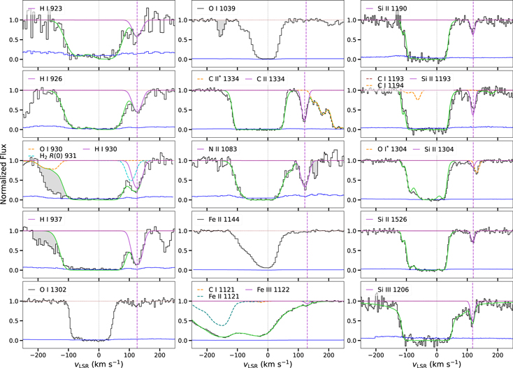
Figure 3. Velocity profiles of the neutral-, low-, and intermediate-ion absorption lines detected toward HD 156359. The normalized flux is shown in black, the continuum level is in red, and the 1σ error in the normalized flux is in blue. The vertical line at 0 km s−1 marks the region associated with the Milky Way. Each of these profiles shows a Voigt fit to the data except for O i, for which we provide an apparent optical depth measurement, and for Fe ii, which is a nondetection. The solid green curve is the overall Voigt-profile fit to the absorption. The magenta curve is the Voigt-profile fit to the HVC absorption feature near +125 km s−1 and the vertical dashed magenta line marks the velocity centroid of the fitted component.
Download figure:
Standard image High-resolution imageTable 2. HD 156359 High-velocity Absorption
| Ion | vLSR | b | log N |
|---|---|---|---|
| (km s−1) | (km s−1) | (N in cm−2) | |
| H i | 125.6 ± 0.9 | 18.9 ± 1.2 | 15.54 ± 0.05 |
| O i | 125.0 ± 4.8 | ⋯ | 12.43 ± 0.11 a |
| Na i | ⋯ | ⋯ | <9.45 b |
| C ii | 120.9 ± 0.6 | 9.8 ± 1.4 | 13.83 ± 0.10 |
| N ii | ⋯ | ⋯ | <13.98 b |
| Si ii | 118.5 ± 1.0 | 7.0 ± 1.6 | 12.94 ± 0.07 |
| Ca ii | 123.7 ± 1.0 | 2.3 ± 2.7 | 10.63 ± 0.10 |
| Fe ii | ⋯ | ⋯ | <12.99 b |
| Si iii | 117.6 ± 1.4 | 6.9 ± 2.8 | 12.32 ± 0.16 |
| Fe iii | 129.3 ± 2.3 | 11.0 ± 3.6 | 12.82 ± 0.14 |
| C iv | 133.3 ± 2.3 | 8.6 ± 3.6 | 12.60 ± 0.13 |
| Si iv | 129.5 ± 1.5 | 5.7 ± 2.9 | 11.93 ± 0.15 |
| N v | 130.2 ± 2.7 | 12.2 ± 4.0 | 12.64 ± 0.11 |
| O vi | 141.3 ± 1.2 | 24.0 ± 1.8 | 13.65 ± 0.03 |
Notes.
a Except where noted, all measurements presented in this table are derived from Voigt-profile fitting, with the exception of O i, for which we derive an apparent column density from the profile in the range +110 ≲ v ≲ + 125 km s−1; see Figure 4. The error listed for log N(O i) is the combination of the statistical error and a continuum-placement error in quadrature, and is ±0.08 ± 0.07 separately. b This measurement is a nondetection and the 3σ limiting column density is given.Download table as: ASCIITypeset image
An important step in measuring H i absorption in FUSE spectra is to decontaminate H2 absorption. Fortunately, the FUSE LiF1 and LiF2 channels provide us with an opportunity to model isolated H2 lines. This allows us to account for the MW’s molecular contribution to the interstellar absorption lines blended with H i in the SiC2A spectrum. We conducted an H2 decontamination, and describe and illustrate this process in detail in Appendix B.
3.3. O i Absorption
After placing a smooth continuum through the O i line at 1302 Å in the STIS E140M spectrum, we noticed a small absorption feature near +125 km s−1 (see Figure 3). This feature spans 5 pixels and has a significance of 3.2σ (EW/σEW = 3.2). Since only one STIS exposure exists, we cannot confirm the O i detection in another data set, and this feature is not seen in the much weaker O i line at 1039 Å in the FUSE spectrum. To explore whether this feature is real, we compared the absorption profile to another low-ion line. Figure 4 shows an apparent column-density profile comparison of the O i 1302 Å line to the weak Si ii 1526 Å line. We chose λ1526 because it is unsaturated, unblended, and seen in a region with high S/N. Although noisier, the profile of O i λ1302 is very similar to Si ii λ1526 in the velocity region near +125 km s−1, and the ratio of their apparent column densities is flat with velocity. To confirm this similarity, the inset plot in Figure 4 shows a linear fit to the ratio over 5 pixels (over two resolution elements) with a slope equal to zero within the margin of error, as expected for a genuine O i detection. Therefore, we proceed with treating the O i λ1302 feature as real on the basis that (1) the line is detected at 3.2σ significance, (2) there is close kinematic consistency with Si ii, and (3) the feature is centered at the same velocity as multiple other ions, e.g., H i, C ii, N ii, and Ca ii. After applying a low and high continuum to this region, we measure log NO i = 12.43 ± 0.08 ± 0.07, which includes the statistical error and a continuum-placement (systematic) error. This measurement is the foundation of our metallicity measurement in the HVC, which we discuss in Section 4.
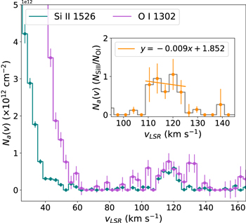
Figure 4. A comparison of the normalized apparent column-density plots between O i 1302 in violet and Si ii 1526 in green. The profiles have similar shapes although the O i 1302 profile shows a lower S/N. The inset panel shows the apparent column-density ratio of Si ii 1526 to O i 1302. A linear fit to 5 pixels in the region from +110 ≲ v ≲ 125 km s−1 has a slope near zero within the margin of error, supporting the reality of the detection in both ions.
Download figure:
Standard image High-resolution image3.4. Low- and Intermediate-ion Absorption
We detected C ii λ1334, Si ii λλ1190, 1193, 1304, 1526, N ii λ1083, Si iii λ1206, and Fe iii λ1122 in the HVC near +125 km s−1 in the FUSE and STIS spectra (see Figure 3). Our absorption-line measurements of these lines are given in Table 2. Achieving a simultaneous Voigt-profile fit using all Si lines is hindered by difficulties in continuum placement for the stronger lines since large spans of the variable stellar continuum are absorbed. Instead, we adopt the Voigt-profile measurement log NSi ii = 12.94 ± 0.07 for the weakest unblended line available at 1526 Å. We show that it is a good fit for λλ1190, 1193, 1304 in Figure 3.
Although detected, N ii 1083 lies in a portion of the FUSE spectrum where the stellar continuum is highly variable over a short range in wavelength. Comparing the neighboring low-velocity H2 J3 1084 Å line to other J3 lines in regions with smooth continua reveals that the continuum must drop significantly in this region, making it difficult to estimate log NN ii . For this reason, our measurement for N ii is an upper limit. Fe ii 1144 has a low absorption profile in the vicinity of the HVC. We applied a high, middle, and low continuum across the absorbing region of λ1144 and calculate a significance of 2.2σ after including a continuum-placement error. We find a 3σ limiting column density of log NFe ii ≤ 12.99; however, given the Fe iii detection in the HVC, we use the Fe iii column density in metallicity calculations going forward. In addition to the high-velocity absorption we observe for Fe iii λ1122, we detect an intermediate-velocity cloud (IVC) centered near +86 km s−1 with log N = 12.98 ± 0.13.
The archival ESO FEROS optical spectrum covers the Ca ii K and H and Na i D lines; see Figure 5. Telluric H2O absorption lines are present in the velocity range of the HVC; however, there is a nondetection of high-velocity Na i, and we find a 3σ limiting column-density limit of log NNa I < 9.45. We see absorption in Ca ii across 6 pixels at 123.7 km s−1 and measure an apparent optical depth (AOD) column density of log NCa II = 10.68 ± 0.01 for Ca ii 3934. We also performed a simultaneous Voigt-profile fit to Ca ii λ3934, 3969 and find log N = 10.63 ± 0.10. The resulting b-value for this small component has a high error. However, since the log N value from Voigt-profile fitting agrees with the AOD measurement within the margin of error, we adopt its value.
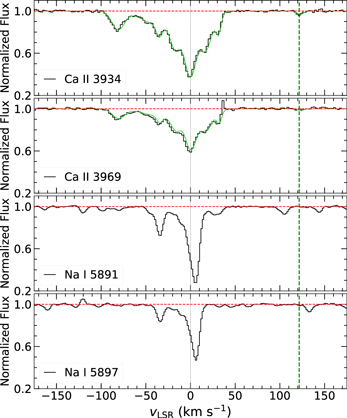
Figure 5. Velocity profiles of the Ca ii λλ3934, 3969 and Na i λλ5891, 5897 absorption lines detected toward HD 156359 in the archival FEROS spectrum. The normalized flux is shown in black, the continuum level is in red. The gray vertical line at 0 km s−1 marks the absorption region associated with the Milky Way. The green curves in the top two panels are the Voigt-profile fits to the data, where the green vertical line at 123.7 km s−1 marks the location of the HVC. There is a nondetection of high-velocity Na i, although telluric H2O absorption lines are present in this region. The lower end of the y-axis begins at +0.2 in all panels to improve the visibility of the absorption features.
Download figure:
Standard image High-resolution image3.5. High-ion Absorption
The C iv and Si iv profiles are complex in the STIS E140M spectrum, showing multiple distinct low- and intermediate-velocity components, in addition to the HVC. The high-ion absorption features for C iv, Si iv, and N v lie on well-defined continua due to their corresponding broad and smooth stellar P Cygni wind profiles, which gradually elevates their stellar continua in the region from −100 to +200 km s−1 for this star, as shown in Figure 6. The high-ion continuum fitting was also guided by fits to the GHRS data previously published by Sembach et al. (1991, 1995).
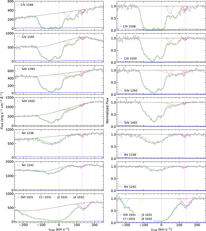
Figure 6. Velocity profiles of the high-ion absorption lines detected toward HD 156359. The flux is shown in black and the 1σ error in the flux is in blue. The dashed black vertical line marks 0 km s−1. The solid green curve is the overall Voigt-profile fit to the absorption. The solid magenta curve is the Voigt-profile fit to the HVC absorption near +130 km s−1 for Si iv, C iv, and N v and near +140 km s−1 for O vi. The vertical dashed magenta line marks the velocity centroid of the fitted component. The pink and yellow curves are fits to components at intermediate velocities.
Download figure:
Standard image High-resolution imageWe detect weak, but significant, absorption in the HVC near +130 km s−1 in C iv λ1548, Si iv λ1393, and N v λλ1238, 1242. We calculated the detection significance in each line by adding the continuum-placement error in quadrature with the statistical (photon-noise) error. We found a 3.6σ significance for the high-velocity C iv λ1548 feature. We observe a slightly weaker feature near +160 km s−1 on the rising C iv λ1548 wind profile, which we attribute to either noise or a detector artifact, as it does not appear in any of the other high ions at the same velocity. The much weaker C iv λ1550 feature falls at the peak of the P Cygni stellar wind profile and we do not detect any significant absorption in the HVC in this line. We measure a 3.2σ significance for the stronger Si iv 1393 feature, but only measure 2.0σ for the weaker Si iv λ1402 line. For the N v λλ1238, 1242 lines, we measure detection significances of 3.0σ and 4.9σ, respectively, where the higher significance for 1242 reflects the high S/N near this line, even though it is intrinsically weaker.
We performed Voigt-profile fitting to C iv, Si iv, and N v high ions with the initial positions of the components and b-values determined from the C iv 1548 Å line. The position and b-values were allowed to vary freely and the results for the fits are given in Table 2. We note the detection of an IVC centered near +78 km s−1 in both C iv and Si iv with log N =13.57 ± 0.08 and 13.09 ± 0.10, respectively.
We observe high-velocity absorption in O vi 1031 and 1037 in the LiF1 channel of the FUSE spectrum at vLSR = 141 km s−1. However, we only include λ1031 in our analysis, because λ1037 lies on the steep blueward side of the O vi P Cygni profile and suffers from significant blending with C ii* 1037 and H2 J1 1038 Å. We measure the O vi λ1031 HVC feature at 7.5σ after including a continuum-placement error.
The wavelength region around O vi 1031 Å contains several absorption lines which can serve as contaminants, most notably HD 6–0 R(0) λ1031.915, Cl i λ1031.507, and several lines of molecular hydrogen including H2 6–0 P(3) λ1031.192 and H2 6–0 R(4) λ1032.351. To gauge the effect of contamination by HD 6–0 R(0) λ1031.915, we examined other HD lines of similar oscillator strength that are isolated from interstellar absorption, such as 5–0 R(0) λ1042.850, 7–0 R(0) λ1021.460, and 8–0 R(0) λ1011.461. We detect no HD molecular absorption in these lines and conclude that no subtraction of the HD 6–0 R(0) line at λ1031.915 from the O vi profile is necessary. For Cl i, a small amount of absorption in Cl i λ1347 is present near 0 km s−1 in the STIS spectrum and we simultaneously fit Cl i λ1031 to derive its contribution to the O vi profile. For molecular hydrogen, H2 6–0 R(4) λ1032.351 is the most relevant potential contaminant as it overlaps with the high-velocity component in O vi λ 1031. We modeled other isolated H2 J4 lines in the FUSE spectrum, e.g., 5–0 R(4) λ1044.543 and 4–0 R(4) λ1057.381 (see description in Appendix B). Through simultaneous fitting of those lines with H2 6–0 R(4) λ1032, we account for the small amount of H2 present in the O vi high-velocity absorption. A similar procedure was followed to account for contamination from H2 6–0 P(3) λ1031.192 near vLSR = −200 km s−1 using the isolated H2 J3 lines 6–0 R(3) λ1028.986 and 5–0 P(3) λ1043.503. The resulting Voigt-profile fit and O vi column density are shown in Figure 6 and Table 2.
4. Results: The Cool Low-ion Gas
The neutral- and low-ionization species, including H i, O i, C ii, N ii, Si ii, Ca ii, Fe ii, Si iii, and Fe iii, trace the cool photoionized phase of the HVC detected at vLSR = +125 km s−1 toward HD 156359. In this section we use the ratios of metal column densities to H i column densities to derive the ion abundances for each observed species in the HVC, as shown in Table 3. The elemental abundances are then derived from the ion abundances using ionization corrections derived from custom photoionization modeling. Finally, a comparison of the relative abundances of different elements is used to derive the dust depletion pattern in the HVC.
Table 3. High-velocity Cloud Elemental Abundances and Depletions
| Ion | [Xi /H i] a | IC(Xi ) b | [X/H] c | δO(X) d |
|---|---|---|---|---|
| O i | 0.20 ± 0.10 | +0.16
|

| 0 |
| C ii | 1.86 ± 0.12 | −1.59 ± 0.04 | 0.27 ± 0.13 | −0.09 ± 0.17 |
| N ii | <2.60 | < − 1.67 | <0.93 | <0.57 |
| Si ii | 1.89 ± 0.08 | −1.86 ± 0.03 | 0.03 ± 0.09 | −0.33 ± 0.14 |
| Fe ii | <1.95 | −1.17
| <0.79 | <0.43 |
| Fe iii | 1.78 ± 0.15 | −1.73 ± 0.08 | 0.06 ± 0.17 | −0.30 ± 0.20 |
| Ca ii | 0.75 ± 0.11 | −0.95 ± 0.01 | −0.20 ± 0.11 | −0.56 ± 0.16 |
Notes.
a Ion abundance [Xi /H i] = log (Xi /H i)HVC − log (X/H)⊙, where Xi is the observed ion of element X. These are not corrected for ionization effects. The error includes both systematic and continuum-placement uncertainties. b Ionization correction IC(Xi ) = [X/H]model − [Xi /H i], derived from the difference between the model elemental abundance and the observed ion abundance. c Ionization-corrected elemental abundance [X/H] = [Xi /H i] + IC(Xi ). Also referred to as gas-phase abundance. d δO(X) ≡ [X/O] = [X/H] − [O/H] is the depletion of element X relative to oxygen.Download table as: ASCIITypeset image
4.1. Photoionization Modeling
To assess the role of photoionization as an ionization mechanism in the HVC, as well as characterize its physical conditions and elemental abundances, we incorporate Cloudy (v.17.02; Ferland et al. 2017) photoionization models into our analysis. We designed a multidimensional grid of models for the low and intermediate ions, assuming they arise in the same gas phase as the H i and are photoionized by the same incident radiation fields. The model assumes a plane-parallel slab of uniform density exposed to both the MW disk-halo radiation field model (Fox et al. 2005, 2014; Barger et al. 2013) and the extragalactic UV background radiation field (Khaire & Srianand 2019). We do not include the effects of ionizing radiation produced by any hot collisionally ionized plasma, which has been shown to also contribute to the photoionization of the gas (Wakker et al. 2012).
The MW disk-halo radiation field is a nonisotropic composite field consisting of hard and soft radiation fields from the escaping UV ionizing flux from O–B stars. The escape fraction for the hard component is derived from the intensity of photoionized Hα emission measured in HVCs at known distances (Bland-Hawthorn & Maloney 1999; Putman et al. 2003), whereas the escape fraction for the soft field is derived from the mean observed opacity of the observed spectrum in the solar neighborhood. At the position of HD 156359 a distance of ∼2.3 kpc below the GC, the magnitude of the escaping hydrogen ionizing flux (log Φ = 5.9) in the MW disk-halo model dominates the extragalactic background radiation by ∼2 orders of magnitude. We consider the degree to which the Cloudy results are sensitive to the magnitude of the ionizing flux by running models with the best-fit magnitude changed by ±0.5 dex (a factor of 3 times higher or lower); see Appendix C.
We ran our models for a grid of metallicity values with [Z/H] varying from −0.5 to +1.5 in steps of 0.1 dex, each over a range of hydrogen number densities log (nH/cm−3) from −3 to 0, in order to explore possible metallicities and densities. We determined the best-fit log nH for each metallicity model by matching the observed column-density ratio of Si iii/Si ii to the model value (see the top panel of Figure C2). The Si iii/Si ii ratio was chosen because both ions have unsaturated detections in the HVC, and using a ratio of adjacent ions from the same element (Si) minimizes metallicity or depletion effects from different metal ions. Using the pairs of metallicity and log nH determined from the Si iii/Si ii ratio, we narrow the range of metallicities by identifying which models are consistent with the observed log NO i = 12.43 ± 0.11, as illustrated in the bottom-left panel of Figure C2. We then run an even finer grid of metallicity values in increments of 0.02 dex over the narrowed metallicity and number density region to determine the range of metallicities and densities allowed by the data.
We find that metallicities in the range 0.18 ≤ [O/H] ≤ 0.51 and densities from −1.69 ≤ log (nH/cm−3) ≤ −1.37 are consistent with the data, giving a model best fit of [O/H] =  at log nH = −1.53 ± −0.16. We repeated this procedure for C ii (see bottom-right panel of Figure C2), which is expected to be weakly depleted (Jenkins 2009), and find that the range 0.21 ≤ [C/H] ≤ 0.42 overlaps with the observed data, giving a model best fit of [C/H] =
  at log nH = −1.49
 . The agreement between the oxygen-based metallicity and the carbon-based metallicity lends support to our methodology and to the robustness of the supersolar metallicity we infer.
We found that repeating this process for a hydrogen ionizing flux ±0.50 dex higher and lower gives a similar best fit of [O/H] = +0.36 and [O/H] = +0.30 ± 0.20, respectively. Thus, our main results are consistent for log Φ = 5.9 ± 0.5. Additionally, we tested whether our choice of radiation field could be influencing our results. To do this, we repeated our suite of models with Cloudy's built-in unextinguished local interstellar radiation field “Table ISM” (Black 1987), which is a commonly used physically motivated field available for modeling interstellar gas, and found [O/H] = +0.23 ± 0.13, again consistent with our main results; see Table C1 and Figure C1 in Appendix C for a detailed description of how we addressed uncertainties in the incident radiation fields by varying their intensity and shape.
The metallicity for this cloud ranks among the highest UV-based metallicities of any HVC observed thus far, along with the HVC at −125 km s−1 toward M5-ZNG1 (l = 39, b =+47
7 at z = +5.3 kpc) with [O/H] = +0.22 ± 0.10 (Zech et al. 2008). M5-ZNG1 was also observed with FUSE and STIS E140M spectra. Their observed metallicity is not corrected for ionization effects, but is likely higher than reported, given the measured low log NH i
= 16.50 ± 0.06 in the cloud and that oxygen shows a positive ionization correction when log N(H i) < 18.5 (Bordoloi et al. 2017). The metallicity of the HD 156359 HVC is also on the high end of the range of <20% to 3 times solar reported by Ashley et al. (2022) in their survey of metallicities of Fermi Bubble HVCs. We note that a supersolar abundance in the inner Galaxy may not be unexpected, given the oxygen abundance gradients reported from emission-line measurements in H ii regions (see Wenger et al. 2019; Arellano-Córdova et al. 2021).
4.2. Ionization Corrections
In ISM abundance work, [O i/H i] is often considered a robust indicator of elemental abundance [O/H], since (1) charge-exchange reactions closely couple the ionization state of hydrogen and oxygen together (Field & Steigman 1971), and (2) oxygen is only lightly depleted onto dust grains (Jenkins2009). However, the assumption that [O i/H i] = [O/H] breaks down when N(H i) is so low that the gas is optically thin or when the ionizing photon flux is extremely high (Viegas 1995). In the HVC at +125 km s−1 toward HD 156359, log N(H i) is only 15.54 ± 0.05, so an ionization correction must be made to account for the column densities of all observed neutral and ion stages.
Our Cloudy models directly provide the ionization corrections for all our observed ion stages. We define the ionization correction as the difference between the model (true) elemental abundance and the observed ion abundance, i.e.,

The resulting ion abundances, ionization corrections, and ionization-corrected elemental abundances are given in Table 3. The relationships between the ionization corrections and the hydrogen number density for [Z/H] = 0.36 are shown in the top panel of Figure 7 and the ionization-corrected abundances are shown in the middle panel of Figure 7.
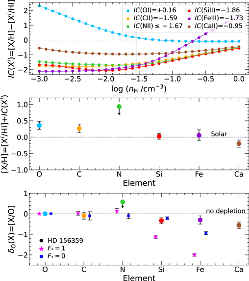
Figure 7. Top: ionization corrections for the low ions O i, C ii, N ii, Si ii, Fe iii, and Ca ii (colored curves) plotted against log nH from our Cloudy model to the HD 156359 HVC. The model uses our best-fit [Z/H] = +0.36. The vertical line marks the best-fit log(nH/cm−3) = −1.53, determined from the Cloudy models for O i (see Figure C2). The ionization correction calculated at −1.53 is added to the observed ion abundance to determine the elemental abundance. Middle: comparison of the ionization-corrected abundances of the low ions detected in the HVC, where the solar abundance is plotted as a horizontal line. Bottom: comparison of the dust depletion levels δ(X) = [X/O] in the HVC with the depletion pattern for [X/O] measured for sight lines with the lowest and highest collective depletions (F* = 0 and F* = 1, respectively) from Jenkins (2009). A slight offset is applied in the x-direction of each element for distinction.
Download figure:
Standard image High-resolution imageThe positive ionization correction of IC(O i) =  from the photoionization modeling results in a high gas-phase oxygen abundance of +0.36. We calculate gas-phase abundances of [C/H] = 0.27 ± 0.13, [N/H] = ≤0.93, [Si/H] = 0.03 ± 0.09, [Fe/H] = 0.06 ± 0.17, and [Ca/H] = −0.20 ±0.11 (see Table 3).
4.3. Dust Depletion Effects
Following convention, we define the depletion δO(X) of each refractory element X as the ionization-corrected abundances of that element compared to the ionization-corrected oxygen abundance, i.e.,

where oxygen represents an undepleted (or lightly depleted) volatile element. In this formalism, a negative value of δO(X) means that element X is depleted relative to oxygen. This method assumes that the total (gas+dust) abundances are solar, which is often assumed to apply to the Galactic ISM (Savage & Sembach 1996), though local ISM abundance variations cannot be ruled out in some sight lines (De Cia et al. 2021). We show δO(X) for the low ions in the bottom panel of Figure 7 compared to F*, the line-of-sight depletion strength factor, for [X/O] determined for low-depletion (F* = 0) and high-depletion (F* = 1) gas from the comprehensive ISM gas-phase element depletions study of Jenkins (2009).
For the HVC toward HD 156359, we find a low value of δO(C) = −0.09 ± 0.17, i.e., carbon shows no significant depletion. This is consistent with the low values of [C/O] measured in Galactic ISM gas (Jenkins 2009). For the other low ions, we find a 3σ upper limit for the nitrogen depletion δO(N) ≤ +0.57 and low depletions for silicon, iron, and calcium of δO(Si) = −0.33 ± 0.14, δO(Fe) = −0.30 ± 0.20, and δO(Ca) = −0.56 ± 0.16, respectively. To summarize the final results of the CLOUDY modeling after the dust depletion levels have been derived, Figure 8 shows the model curves of the detected ions shifted by their respective depletions at [X/H] = +0.36 and log nH = −1.53. The ability of this model to match the observed column densities shows that all low-ion measurements can be explained by photoionization once dust depletion effects are accounted for.
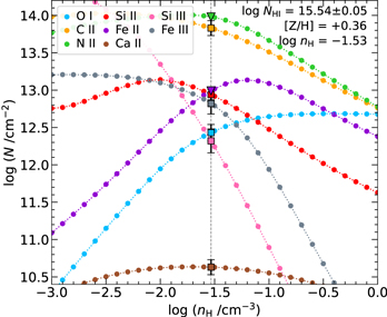
Figure 8. Our final Cloudy photoionization model of the low and intermediate ions detected in the HVC toward HD 156359 near +125 km s−1. The model uses the best-fit [Z/H] = +0.36 determined from our O i analysis. These model predictions for each ion (colored dotted curves) have been scaled by the dust depletions required to match the observed values, where the observed column densities are indicated by circle markers at the best-fit log (nH/cm−3) = −1.53 (black vertical line).
Download figure:
Standard image High-resolution imageA low level of dust depletion for the HVC is consistent with the well-known Routly–Spitzer (RS) effect, in which the amount of dust observed in HVCs decreases significantly at higher LSR velocity (see Routly & Spitzer 1952; Siluk & Silk 1974; Vallerga et al. 1993; Smoker et al. 2011; Ben Bekhti et al. 2012; Murga et al. 2015). The RS effect is typically traced by the N(Na i)/N(Ca ii) ratio, which has been found to significantly decrease with increasing LSR velocity. Although the RS effect was historically interpreted as a dust depletion effect, it may also be related to ionization effects, and likely differs depending on the environment of the cloud. We measure an 3σ upper limit of log N(Na i)/N(Ca ii) ≤ −1.2 in the +124 km s−1 HVC toward HD 156359 from the optical FEROS data, which is on the low end of the observed ratios for HVCs (Smoker et al. 2011; Ben Bekhti et al. 2012; Murga et al. 2015), and is also lower than is typically observed at low velocities. In summary, the dust depletion pattern we derive in the HVC is consistent with other HVCs and with the RS effect, even though the cloud has high metallicity.
5. Results: The Highly Ionized Gas
The HVC toward HD 156359 shows significant, yet weak, high-ion absorption in the stronger lines from the resonance doublets of Si iv and C iv, and in both lines of the N v doublet near vLSR = 130 km s−1. We also detect stronger O vi at a slightly higher velocity of 141 km s−1 (Figure 6; Table 2). To compare the high-ion absorption between different ions, we show in Figure 9 a comparison of the normalized optical depth profiles of each high ion. These plots provide a way to intercompare the profiles of different ions in a linear manner (e.g., Fox et al. 2003). The HVC line profiles of C iv and Si iv are well aligned in velocity, but are offset from the centroid of O vi absorption by ≈8 km s−1. This suggests that the O vi exists in a separate (likely hotter) gas phase. The STIS profile of N v is too noisy to draw any conclusions about line centroid. However, the GHRS N v profiles (Sembach et al. 1995) are less noisy and have a similar profile shape to the O vi seen in the FUSE data, supporting the placement of O vi and N v in the same phase.
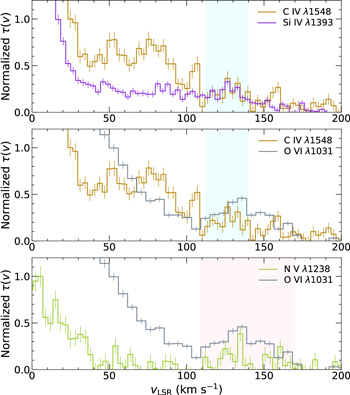
Figure 9. Optical depth profiles of the high ions, where each profile is arbitrarily normalized to its peak value for the velocity region shown in order to facilitate comparison. Top panel: C iv λ1548 and Si iv λ1393 display similar line shapes in the velocity region of the HVC from 112 ≲ v ≲ 140 km s−1, indicated with cyan shading. Middle panel: C iv λ1548 and O vi λ1031 are compared, where the center of the HVC absorption for O vi is shifted to a higher velocity at v ≈ 141 km s−1. Bottom panel: N v λ1238 and O vi λ1031 are compared, where the range of velocities attributed to absorption by O vi are indicated in light pink.
Download figure:
Standard image High-resolution image5.1. Collisional Ionization Modeling
The observed high ions have column densities that are too high to be explained by the Cloudy photoionization models described in Section 4.1. Although these models do not include energetic photons from the radiation field intrinsic to the Fermi Bubbles or in situ ionizing photons from the hot gas itself, which could partially contribute to the photoionization of the C iv and Si iv gas, the models underproduce the observed Si iv and C iv column densities by ∼0.7 and 1.0 dex, respectively. The N v and O vi column densities are underproduced by orders of magnitudes (see Table C1). These discrepancies imply that a separate ionization mechanism is likely required for C iv and Si iv, and is definitely required for N v and O vi. Here, we explore collisional ionization in gas with temperatures of T ≳ 105 K as the separate mechanism. We consult the collisional ionization models from Gnat & Sternberg (2007) to determine the exact range of temperatures allowed by the high-ion column densities and their ratios. While we considered the more recent models from Gnat (2017) that include photoionization effects from the extragalactic UV background, we do not adopt them because HD 156359 lies in close proximity to the radiation field of the Galactic plane, which is much stronger. We considered both the collisional ionization equilibrium (CIE) and nonequilibrium regimes.
A single-temperature solution explaining all four high ions (Si iv, C iv, N v, O vi) in the HVC is ruled out, as no such solution exists to the observed high-ion column densities. Instead, we find that a two-phase solution is needed, with one temperature explaining the NC iv /NSi iv ratio and another explaining NO vi /NN v . This two-phase model is consistent with the kinematic information in the UV spectra, where Si iv and C iv show very similar line profiles but O vi is offset in velocity centroid. The two-phase high-ion model is illustrated in Figure 10, which shows the observed high-ion ratios of NC iv /NSi iv and NO vi /NN v compared to model predictions from Gnat & Sternberg (2007) for solar ([Z/H] = 0) and supersolar ([Z/H] = +0.3) metallicities.
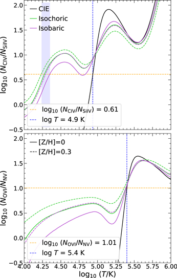
Figure 10. Comparison of observed high-ion column-density ratios with predictions from the collisional ionization models of Gnat & Sternberg (2007). The observed ratios in the HD 156359 HVC are shown as dashed orange horizontal lines. The top and bottom panels show the C iv/Si iv and O vi/N v ratios, respectively. In both panels, the solid black curve is the collisional ionization equilibrium model ion fraction. The solid green and violet curves are the time-dependent isochoric and isobaric collisional ionization models for a solar metallicity, respectively. Their dashed counterparts are the same but for a metallicity twice the solar value. The vertical dashed blue line is the temperature of the gas determined by the models. The vertical blue band in the top panel represents a second time-dependent solution for a range of temperatures from log T = 4.2–4.4 K.
Download figure:
Standard image High-resolution imageFor the C iv/Si iv phase, we find two possible solutions for the temperature. First, the nonequilibrium isochoric (constant volume) and isobaric (constant pressure) models give a low-temperature solution at T = 104.2−4.4 K, where the lower end corresponds to the solar-metallicity isochoric model and the higher end with the supersolar isobaric model. Second, the CIE model returns a higher temperature T = 104.9 K. We are inclined to adopt the nonequilibrium (lower-temperature) solution, as plasma near T = 105 K is at the peak of the cooling curve, where oxygen dominates the radiative cooling and the gas can cool faster than it recombines, reaching a nonequilibrium state. For the O vi/N v phase, a single-temperature solution for the observed log NO vi /NN v = 1.01 is found at T = 105.4 K for all models (see bottom panel of Figure 10).
In conclusion, we can successfully model the high-ion plasma in the HVC toward HD 156359 as containing collisionally ionized gas at two temperatures: a cooler phase seen in C iv and Si iv at T = 104.2−4.4 K, and a hotter phase seen in N v and O vi at T = 105.4 K. We note that the velocity offset of ∼20 km s−1 for O vi from the low ions is consistent with offsets on the order of tens of kilometers per second predicted by conductive interface models of evaporation between hot and cool gas (Bohringer & Hartquist 1987; Borkowski et al. 1990) or from models for dynamical cooling flows (Wakker et al. 2012). Given the small velocity centroid uncertainties from the Voigt-profile modeling (∼1–5 km s−1; see Table 2), the ∼20 km s−1 offset is significant and could indicate we are tracing hot gas in an interface layer moving at a higher velocity than the cooler gas inside the cloud.
6. Summary
Using archival FUSE, HST STIS, and ESO FEROS spectra, we have analyzed the chemical composition of the HVC near +125 km s−1 toward HD 156359, a massive star lying 9 kpc away toward the GC. The sight line passes less than 1° from one of the densest cores of a complex of small HVCs, dubbed “Complex WE” by Wakker & van Woerden (1991), as shown in Figure 1. Furthermore, the sight line passes through a region of enhanced X-ray emission (the southern eROSITA Bubble; Predehl et al. 2020), which indicates energetic feedback from the GC. Our main results are as follows.
- 1.We determined an H i column density of log N(H i) = 15.54 ± 0.05 in the HVC using unsaturated Lyman series absorption lines.
- 2.We measured a supersolar O i abundance of [O i/H i] = 0.20 ± 0.11 in the HVC. After applying an ionization correction derived from a customized photoionization model, we derive an oxygen abundance of [O/H] = 0.36 ± 0.12, indicating the cloud is enriched to 1.7–3.0 times the solar level. This abundance is consistent with the supersolar oxygen abundances of H ii regions measured in the inner Galaxy (Wenger et al. 2019; Arellano-Córdova et al. 2021).
- 3.
- 4.A low level of dust depletion is inferred from the silicon, iron, and calcium lines, with [Si/O] = −0.33 ± 0.14, [Fe/O] = −0.30 ± 0.20, and [Ca/O] = −0.56 ± 0.16. The Na i/Ca ii ratio in the HVC is ≤−1.2, lower than is typically observed at low velocities, consistent with the trend known as the RS effect.
- 5.We detect high-ion absorption in C iv, Si iv, N v, and O vi near +130 km s−1, at slightly higher velocities than the velocity range of the lower ions. Our ionization modeling shows that a mechanism separate from photoionization, such as collisional ionization, is required to explain the column densities of the high ions. We determine that a two-phase temperature solution best explains the observed NC iv /NSi iv and NO vi /NN v ratios, with a cooler phase seen in C iv and Si iv at T = 104.2−4.4 K, and a hotter phase seen in N v and O vi at T = 105.4 K.
The high metallicity, low depletion, complex high-ion absorption, and high positive velocity of the HVC toward HD 156359 are all consistent with a wind origin, in which a swept-up clump of material is being carried out from the Galactic disk into the halo. As such, this HVC may represent a freshly entrained cool clump of gas caught in the act of being accelerated into the nuclear wind. While we cannot rule out a foreground origin for the HVC, in which the cloud exists at an anomalous velocity somewhere between the Sun and the GC, we can exclude a spiral-arm explanation for the HVC on kinematic grounds, because the cloud’s +125 km s−1 velocity lies over 100 km s−1 away from the nearest spiral arm, the Sagittarius Arm at ∼−10 km s−1. Under a biconical outflow model (Fox et al. 2015; Bordoloi et al. 2017; Di Teodoro et al. 2018), the cloud’s radial velocity and its location only 2.3 kpc below the disk imply a short timescale of ∼5 Myr for the HVC to have reached its current position, which is much shorter than the timescales on which chemical mixing is expected to be significant (tens to hundreds of millions of years; Gritton et al. 2014; Heitsch et al. 2022). Our observations therefore provide a snapshot into the chemical and physical conditions prevailing in this early stage of a nuclear outflow, before chemical mixing has diluted or enriched the gas from its initial state.
We gratefully acknowledge the invaluable contributions to early versions of this manuscript from the late Blair Savage, who passed away during the manuscript’s preparation. This paper would not have been possible without Blair’s foundational work on the HD 156359 sight line, the chemical abundances in the ISM, apparent optical depth analysis, and the inner Galaxy. We gratefully acknowledge support from the NASA Astrophysics Data Analysis Program (ADAP) under grant No. 80NSSC20K0435, “3D Structure of the ISM toward the Galactic Center.” The FUSE data were obtained under program P101. FUSE was operated for NASA by the Department of Physics and Astronomy at the Johns Hopkins University. D.K. is supported by an NSF Astronomy and Astrophysics Postdoctoral Fellowship under award AST-2102490. We thank Isabel Rebollido for valuable conversations on the FEROS spectrograph. The FUSE and HST STIS data presented in this paper were obtained from the Mikulski Archive for Space Telescopes (MAST) at the Space Telescope Science Institute. The ESO FEROS spectrum was obtained from the ESO Archive Science Portal.
The FUSE and HST STIS data presented in this paper were obtained from the Mikulski Archive for Space Telescopes (MAST) at the Space Telescope Science Institute. The specific observations analyzed can be accessed via 10.17909/rrnk-3e58.
Facilities: FUSE - Far Ultraviolet Spectroscopic Explorer satellite, HST(STIS) - , ESO(FEROS) - .
Software: astropy (Astropy Collaboration et al. 2018), Cloudy (Ferland et al. 2017), linetools (Prochaska et al. 2017), VPFIT (Carswell & Webb 2014), CalFUSE (Dixon & Kruk 2009), calSTIS (Dressel et al. 2007), FEROS-DRS (Kaufer et al. 1999).
Appendix A: Global Continuum Fitting
Stellar absorption lines present a continuum-fitting challenge, particularly in the complex far-UV FUSE spectra used to derive the H i column density in the HVC under study. Our approach followed in the analysis is to fit the continuum locally around each H i Lyman series line of interest, since this allows us to account for stellar absorption lines, which are present in the continuum when the radiation field encounters the HVC. However, for completeness here we consider a global continuum-fitting process, which fits the H i continuum over a larger range (916–944 Å) in the SiC2 channel. This approach neglects stellar absorption features but ensures the continua are continuous between adjacent lines in the Lyman series. Wavelength regions free from stellar emission and absorption lines defined the flux of the global continuum. We show a global fit to the stellar flux in the vicinity of the higher-order H i Lyman series lines in Figure A1, in which areas of emission and absorption due to both stellar and interstellar features can be seen. We performed a simultaneous Voigt-profile fit on the same H i lines modeled with the global continua, using the mid-, high-, and low-continuum fits shown in Figure A1. A separate local continuum was applied to the depressed region resulting from stellar line blanketing and which contains H i λ923. Using the global continuum fit (which has a slightly higher continuum placement than the local fits) results in log NH i = 15.69 ± 0.03 ± 0.03 for the HVC, where the first error is the statistical error due to photon noise and the second error is the systematic continuum-placement error. This corresponds to a moderate difference of Δlog NH i = 0.15 dex between the H i column densities derived by the global and local continuum methods.
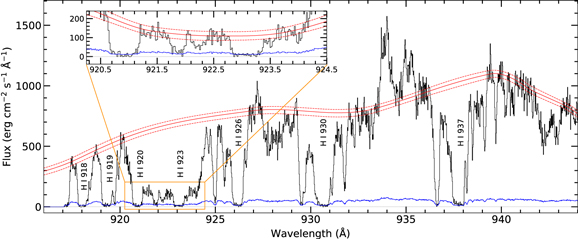
Figure A1. A portion of the FUSE SiC2 spectrum from 916 to 944 Å in which several higher-order H i Lyman series lines are identified. The flux and 1σ error in the flux are shown in black and blue, respectively. A global fit to the stellar continuum is traced by a solid red curve, with a high and low stellar continuum placement marked by dashed red lines. The orange box shows a local fit to a depressed portion of the stellar continuum created by stellar line blanketing, from ∼920 to 925 Å.
Download figure:
Standard image High-resolution imageAppendix B: Decontamination of Molecular Hydrogen
The FUSE LiF1 and LiF2 channels provide us with an opportunity to model isolated H2 lines. This effort is important because it enables us to account for the MW’s molecular contribution to the interstellar absorption lines. In particular, contamination from MW H2 affected the higher-order Lyman series H i in the SiC2A channel and O vi in the LiF1 channel. We performed simultaneous single-component Voigt-profile fits to multiple H2 transitions from rotational levels J = 0–6, allowing both the velocity and b-value to vary freely for the stronger J = 0–4 transitions. The b-values of the significantly weaker J = 5, 6 transitions were fixed to the b-value of the J = 4 transition in order to deter unrealistic column densities for these fainter lines. These results of these fittings are shown in Figure B1.
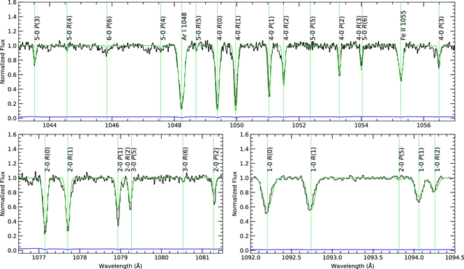
Figure B1. We performed Voigt-profile fits to vibrationally and rotationally excited H2 lines from the FUSE LiF1 and LiF2 channels in order to account for molecular blending with H i. In each panel, the flux and 1σ error in the flux are shown in black and blue, respectively. Voigt-profile fits to the data are shown in green. Green vertical lines mark the positions of the H2 absorption lines. Top panel: LiF1 channel H2 transitions from upper vibrational levels 4 and 5, spanning rotational levels J = 0 − 6. Fits to Ar i λ1048 and Fe ii λ1055 are included. Bottom-left panel: LiF1 channel H2 transitions from upper vibrational levels 2 and 3, including rotational levels J = 0, 1, 2, 5, 6. Bottom-right panel: LiF2 channel H2 transitions from upper vibrational levels 1 and 2, including rotational levels J = 0, 1, 2, 5.
Download figure:
Standard image High-resolution imageAppendix C: Supplemental Cloudy Data
In order to assess the role of photoionization in explaining our HVC column densities and to model the elemental abundances of the gas, we used the spectral synthesis code Cloudy (v.17.02, Ferland et al. 2017), which is designed to simulate physical and chemical conditions in the ISM. Since the sight line toward HD 156359 passes through (or close to) the energetic environment of the Galactic nuclear wind, it is important to design a model that accurately reflects the unique conditions of this region.
Currently, the most accurate representation of the escaping ionizing flux from the MW is the disk-halo model (Bland-Hawthorn & Maloney 1999; Fox et al. 2005, 2014; Bland-Hawthorn et al. 2019). This nonisotropic field accounts for spatial variations in the photon escape fraction and shows stronger radiation emerging near the GC than at larger radii. The disk-halo model predicts an ionizing photon flux log Φ = 5.9 photons cm−2 s−1 at the position of HD 156359, thus we adopt this value as the best-fit intensity of the field. The spectral shape of the field and both the unextinguished and position-selected (extinguished) intensity are shown in Figure C1, with the model results for the best fit log Φ = 5.9 shown in Figure C2. We explored the sensitivity of our models to the field intensity by repeating our suite of models with a radiation field 0.5 dex lower and higher than the best-fit log Φ = 5.9, where 0.5 dex was chosen because the disk-halo contours are given in 1 dex intervals, so 0.5 dex is a suitable subgrid uncertainty. The results of the models at log Φ = 5.4, 5.9, and 6.4 are shown in the first three columns of Table C1. We find that the oxygen abundance and ionization correction are consistent within errors in all three models, showing that the output metallicity is insensitive to the strength of the radiation field. The high-ion deficits, defined as log N(observed)–log N(model) for each high ion, are also largely unchanged between the three models. These deficits are substantial for the three models for all four high ions under study (Si iv, C iv, N v, and O vi), with the deficit rising with increasing ionization potential (smallest for Si iv, biggest for O vi), and generally rising with increasing ionizing flux. The existence of these deficits is the basis of our claim that the high ions are collisionally ionized.
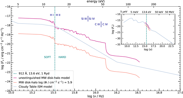
Figure C1. A comparison of intensity vs. frequency for the incident radiation fields used in the Cloudy models. The pink curve shows the shape and intensity of the unextinguished Milky Way disk-halo radiation field (Bland-Hawthorn & Maloney 1999; Fox et al. 2005, 2014; Bland-Hawthorn et al. 2019), where the peach curve shows the same field at the position of HD 156359 at log (Φ/cm−2 s−1) = 5.9. The gray curve is the unextinguished Cloudy built-in local interstellar radiation field “Table ISM” (Black 1987), with the entire field shown in the inset plot. The vertical dashed green line marks the H i ionization edge at 912 Å (13.6 eV). The Si iii and C iii ionization edges are marked by short vertical blue lines at 33.5 and 47.9 eV, respectively.
Download figure:
Standard image High-resolution imageTable C1. Summary of Results from Cloudy Models: Oxygen Abundances and High-ion Deficits
| Milky Way Disk-halo Spectral Energy Distribution | Cloudy Spectral Energy Distribution | |||
|---|---|---|---|---|
| log Φ = 5.9 | log Φ = 5.4 | log Φ = 6.4 | Table ISM | |
| [O/H] |
+0.36

| +0.30 ± 0.20 | +0.36
| +0.23 ± 0.13 |
| IC(O) |
+0.16

| +0.10 | +0.16 | +0.03 |
| Δlog N(Si iv) | 0.67 | 0.66 | 0.75 | 1.02 |
| Δlog N(C iv) | 0.99 | 1.09 | 1.00 | 1.69 |
| Δlog N(N v) | 3.74 | 3.65 | 4.08 | 4.58 |
| Δlog N(O vi) | 8.35 | 8.07 | 8.91 | 13.65 |
Note. This table shows the key results (oxygen abundance, oxygen ionization correction, and high-ion deficit) from four Cloudy models, to illustrate the effect of changing the intensity and shape of the radiation field. The first three columns show models using the disk-halo radiation field (Bland-Hawthorn & Maloney 1999; Fox et al. 2005, 2014; Bland-Hawthorn et al. 2019) at three different ionizing fluxes, with our adopted model shown in bold. The fourth column shows the model using Cloudy's built-in interstellar radiation field “Table ISM” (Black 1987). The high-ion deficits are defined as log N(observed)–log N(model).
Download table as: ASCIITypeset image
Additionally, we gauged how the shape of the radiation field could be affecting our results. We repeated our suite of models with Cloudy's built-in unextinguished local interstellar radiation field “Table ISM” (Black 1987) instead of the disk-halo field. Table ISM is appropriate for the general ISM and is the most physically motivated field available. Figure C1 shows both the shape and intensity of this field compared to the MW disk-halo model. Although Table ISM has a high-energy tail, its slope is steeper than the disk-halo field in the wavelength region common to both fields, indicating it is a softer field, with an lower ratio of high-energy photons to low-energy photons. Although harder fields are available in Cloudy, such as “Table AGN,” we did not explore a harder field given that the MW’s AGN is not currently active. The last column of Table C1 summarizes the results of the models using “Table ISM.” Using the Table ISM field, we find the HVC has [O/H] = +0.23 ± 0.13, which agrees with the metallicity from our adopted best-fit model within the margin of error. The high-ion deficits are even larger for the Table ISM model than for the three disk-halo models.
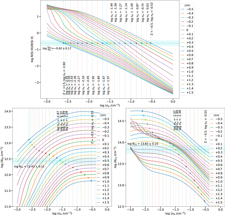
Figure C2.
Cloudy photoionization models of the HVC toward HD 156359 that explore a parameter space in metallicity and number density, −0.50 ≤ [Z/H] ≤ +1.50 and −3 ≤ log (nH/cm−3) ≤ 0, respectively. Top panel: model results for log NSi iii
/NSi ii
for the set metallicities are shown as solid colored curves. The dashed horizontal turquoise line is the observed ratio of −0.62 ± 0.17. The best-fit log nH for each metallicity model is determined by the intersection of the model and observed ratio and is marked by vertical colored lines and circle markers. Bottom-left panel: the model curves for log NO i
for each metallicity are plotted against log nH, where the values derived from log NSi iii
/NSi ii
are marked with vertical lines and markers. The horizontal turquoise line and bar show the observed log NO i
= 12.43 ± 0.11. The model data corresponding to the metallicity region from +0.18 ≤ [Z/H] ≤ +0.51 and −1.69 ≤ log nH ≤ −1.37 overlap with the observed data. The model best-fit values are [Z/H] = +0.36 and log nH = −1.53 ± 0.16. Bottom-right panel: same as for the bottom-left panel but for C ii. The horizontal turquoise line and bar show observed log NC ii
= 13.83 ± 0.10. The model data corresponding to the metallicity region from +0.21 ≤ [Z/H] ≤ +0.42 and −1.59 ≤ log nH ≤ −1.40 overlap with the observed data. The model best-fit values are [Z/H] = +0.30
and log nH = −1.53 ± 0.16. Bottom-right panel: same as for the bottom-left panel but for C ii. The horizontal turquoise line and bar show observed log NC ii
= 13.83 ± 0.10. The model data corresponding to the metallicity region from +0.21 ≤ [Z/H] ≤ +0.42 and −1.59 ≤ log nH ≤ −1.40 overlap with the observed data. The model best-fit values are [Z/H] = +0.30 and log nH =
  .
.
Download figure:
Standard image High-resolution image