Abstract
Eruptive mass loss of massive stars prior to supernova (SN) explosion is key to understanding their evolution and end fate. An observational signature of pre-SN mass loss is the detection of an early, short-lived peak prior to the radioactive-powered peak in the lightcurve of the SN. This is usually attributed to the SN shock passing through an extended envelope or circumstellar medium. Such an early peak is common for double-peaked Type IIb SNe with an extended hydrogen envelope but uncommon for normal Type Ibc SNe with very compact progenitors. In this paper, we systematically study a sample of 14 double-peaked Type Ibc SNe out of 475 Type Ibc SNe detected by the Zwicky Transient Facility. The rate of these events is ∼3%–9% of Type Ibc SNe. A strong correlation is seen between the peak brightness of the first and the second peak. We perform a holistic analysis of this sample’s photometric and spectroscopic properties. We find that six SNe have ejecta mass less than 1.5 M⊙. Based on the nebular spectra and lightcurve properties, we estimate that the progenitor masses for these are less than ∼12 M⊙. The rest have an ejecta mass >2.4 M⊙ and a higher progenitor mass. This sample suggests that the SNe with low progenitor masses undergo late-time binary mass transfer. Meanwhile, the SNe with higher progenitor masses are consistent with wave-driven mass loss or pulsation-pair instability-driven mass-loss simulations.
Original content from this work may be used under the terms of the Creative Commons Attribution 4.0 licence. Any further distribution of this work must maintain attribution to the author(s) and the title of the work, journal citation and DOI.
1. Introduction
Most massive stars undergo mass loss during their lifetime. This can affect the star's luminosity, burning lifetime, apparent temperature, and helium-core mass and impact its end fate. The mass loss has a great influence on the late-time evolution of massive stars and the resultant supernova (SN; e.g., Smith 2014). Pre-SN mass loss also has an impact on other areas of astronomy since it affects predictions for ionizing radiation, wind feedback from stellar remnants, and the origin of compact stellar remnants.
Early observations of SNe and theoretical models indicate that enhanced mass loss and pre-SN outbursts may occur in progenitors of many types of core-collapse SNe (CCSNe). Different evidence includes the direct detection of precursor outbursts (Pastorello et al. 2007; Strotjohann et al. 2015, 2021, 2024; Jacobson-Galán et al. 2022a), bright UV emission in Type IIP SNe at early times (e.g., Morozova et al. 2018; Bostroem et al. 2019), and narrow spectral lines originating from a dense circumstellar medium ionized by the explosion's shock (as in Type IIn, Type Ibn, Type Icn, and Type II SNe; e.g., Pastorello et al. 2008; Smith 2017; Bruch et al. 2021; Perley et al. 2022). Various mechanisms have been proposed to explain this mass loss, like standard nuclear burning instabilities and gravity waves (Arnett & Meakin 2011; Quataert & Shiode 2012; Leung et al. 2021b; Wu & Fuller 2021, 2022a), silicon deflagration (Woosley & Heger 2015), radiation-driven steady winds (Crowther 2007), pulsation-pair instability-driven mass loss (Leung et al. 2019), and binary interactions (Wu & Fuller 2022b).
The detection of the first peak in the lightcurve of a double-peaked SN constitutes an observational signature of circumstellar matter (CSM) or an extended envelope around the progenitor. If strong mass loss occurred shortly before the SN explosion, it would create a layer of CSM around the SN progenitor. The shock-cooling emission (i.e., bright postbreakout emission; Rabinak & Waxman 2011; Nakar & Piro 2014; Piro 2015; Waxman & Katz 2017; Piro et al. 2021; Khatami & Kasen 2023; Morag et al. 2023) is seen as the SN shock passes through this ejected material. This should manifest as an early peak in the SN lightcurve. This is common for Type IIb SNe, where the extended material is attributed to the outer He/H envelope. However, the progenitors of Type Ib and Ic SNe (SNe Ibc) are suggested to be very compact Wolf–Rayet (W-R) stars or helium stars whose hydrogen envelopes have been stripped off via mass loss (e.g., Yoon 2015). Eruptive mass loss prior to an SN explosion could provide a medium for the shock to propagate through.
This early peak has been detected in a few Type Ibc SNe in the past. The presence of CSM is likely responsible for the first peak of several peculiar SNe Ic, like SN 2006aj (Modjaz et al. 2006), SN 2010mb (Ben-Ami et al. 2014), iPTF 15dtg (Taddia et al. 2016), and SN 2020bvc (Ho et al. 2020), and double-peaked superluminous SNe Ic (e.g., PTF 12dam, Vreeswijk et al. 2017; LSQ 14bdq, Nicholl et al. 2015; Nicholl & Smartt 2016; DES 14X3taz, Smith et al. 2016). The double peak is also seen in a few ordinary Type Ibc SNe, such as SN LSQ 14efd (Barbarino et al. 2017), iPTF 16hgs (De et al. 2018), SN 2017ein (Xiang et al. 2019), SN 2018lqo (De et al. 2020), SN 2019ehk (Jacobson-Galán et al. 2020; De et al. 2021; Nakaoka et al. 2021), SNe 2021gno and 2021inl (Jacobson-Galán et al. 2022b), and SN 2022oqm (Irani et al. 2024), and ultrastripped SNe (USSNe), such as SN 2019dge (Yao et al. 2020) and iPTF 14gqr (De et al. 2021). The low number of detections could be because of an observational bias, as the detection of these sources requires a fast cadence and early follow-up.
Modern high-cadence surveys such as the Zwicky Transient Facility (ZTF; Bellm et al. 2019a; Graham et al. 2019; Masci et al. 2019) act as a discovery engine for such events. In this paper, we present a sample of 17 double-peaked Type Ibc SNe detected by the ZTF. These detections are part of the Census of the Local Universe (CLU) survey (De et al. 2020) and the Bright Transient Survey (BTS; Fremling et al. 2020; Perley et al. 2020). The CLU survey is designed as a volume-limited survey with the objective of classifying all SNe within 200 Mpc whose host galaxies are part of the CLU galaxy catalog (Cook et al. 2019). BTS is a magnitude-limited survey focused on spectroscopically classifying SNe with a peak magnitude brighter than 18.5 mag. In this paper, we perform a holistic analysis of the lightcurves for both the shock-cooling and the radioactive peaks, as well as for early-time, photospheric, and nebular spectra of the sample. Based on the estimated CSM and progenitor properties, we provide constraints on the mass loss and progenitor channels.
The sample selection is described in Section 2. We describe the photometric and spectroscopic data in Section 3. We present our analysis and results from the spectra and the lightcurves in Section 4. We discuss the inferred progenitor masses in Section 5 and the mass-loss scenarios in Section 6. We provide a brief summary of the results and future goals in Section 7.
2. Sample Selection
In this paper, we use SNe observed by the ZTF. The ZTF camera (Dekany et al. 2020) is mounted on the Palomar 48 inch (P48) Oschin Schmidt telescope and has a field of view spanning 47 deg2. ZTF images the entire northern sky every ∼2 nights in the g and r bands and achieves a median depth of approximately 20.5 mag (Bellm et al. 2019b). We use ZTF discoveries and follow-up spectra that are part of the BTS and the CLU survey.
We apply the following selection criteria on the ZTF SN sample obtained from the BTS and the CLU survey (2018 April 1–2022 October 25).
1. The transient should be classified as a stripped-envelope SN (SESN; Types Ib, Ib-pec, Ibn, Ic, Ic-pec, Icn, and Ic-BL, but Type IIb are not included) based on photospheric spectral template matching and manual inspection. As per the classification status on 2022 October 25, there are 185 SNe classified as Type Ib, 27 classified as Type Ibn, 176 classified as Type Ic, 59 classified as Type Ic-BL, and 28 classified as Type Ib/c with unclear type (S. Yang et al. 2024, in preparation).
2. In our analysis, we utilize the ZTF forced-photometry service developed by Masci et al. (2019) to perform forced photometry in the g, r, and i bands on the ZTF difference images. We consider 3σ measurements as a threshold. A total of 59 Type Ib/Ibn SNe, 86 Type Ic/Icn/Ic-BL SNe, and 47 Type Ib/c SNe (classification not distinguishable between Ib and Ic) have good-quality early-time lightcurves, where the gap between the first and second detection, as well as the gap between the last nondetection and the first detection, is less than 5 days. Hence, we did not miss the first peak for these SNe.
3. We manually inspect the lightcurves of these transients to look for an early bump with a rise and decline or just a decline in either of the ZTF g-band or r-band photometry followed by a second peak. We find 19 such SNe, with 10 Type Ib, 4 Type Ic, 3 Type Ic-BL, and 2 Type Ib/c. We list the details of the sample in Table 1.
Table 1. Summary of the Sample of 17 SNe Used in This Paper
| ZTF Name | IAU Name | R.A. | Decl. | Redshift | Type |

| Mr1 |

| Mr2 | AV,MW | AV,host |
|---|---|---|---|---|---|---|---|---|---|---|---|
| (hh:mm:ss) | (dd:mm:ss) | (MJD) | (mag) | (MJD) | (mag) | (mag) | (mag) | ||||
| ZTF21aaqhhfu a | SN 2021gno | 12:12:10.29 | +13:14:57.0 | 0.006 | Ib | 59294 | −14.5 | 59306 | −15.2 | 0.10 | 0 |
| ZTF21abcgnql | SN 2021niq | 15:36:06.70 | +43:24:21.4 | 0.018 | Ib | 59362 | −15.1 | 59371 | −15.8 | 0.07 | 0 |
| ZTF20abbpkng | SN 2020kzs | 17:14:55.02 | +35:31:13.6 | 0.037 | Ib | 58983 | −17.5 | 59009 | −18.7 | 0.08 | 1.1 |
| ZTF21abccaue | SN 2021nng | 14:17:22.86 | +58:44:58.9 | 0.040 | Ib | 59336 | −16.5 | 59381 | −18.4 | 0.03 | 0.6 |
| ZTF18achcpwu | SN 2018ise | 07:07:16.74 | +64:03:41.8 | 0.055 | Ic | 58423 | −16.7 | 58455 | −18.6 | 0.11 | 0 |
| ZTF18abmxelh | SN 2018lqo | 16:28:43.25 | +41:07:58.6 | 0.033 | Ib | 58340 | −15.8 | 58354 | −16.4 | 0.02 | 0 |
| ZTF21acekmmm | SN 2021aabp | 23:09:55.08 | +09:41:08.9 | 0.064 | Ic-BL | 59486 | −18.3 | 59505 | −19.1 | 0.15 | 0 |
| ZTF21aasuego a | SN 2021inl | 13:01:33.24 | +27:49:55.0 | 0.018 | Ib | 59311 | −14.8 | 59321 | −14.8 | 0.02 | 0 |
| ZTF21abdxhgv | SN 2021qwm | 15:18:25.73 | +28:26:04.1 | 0.070 | Ib/c | 59369 | −17.1 | 59395 | −18.8 | 0.07 | 0 |
| ZTF22aapisdk | SN 2022nwx | 22:15:43.95 | +37:16:47.0 | 0.020 | Ib | 59755 | −15.8 | 59764 | −15.9 | 0.41 | 0 |
| ZTF22aasxgjp b | SN 2022oqm | 15:09:08.21 | +52:32:05.1 | 0.011 | Ic | 59772 | −16.3 | 59785 | −17.3 | 0.05 | 0 |
| ZTF21aacufip | SN 2021vz | 15:21:26.85 | +36:46:04.0 | 0.045 | Ic | 59223 | −17.5 | 59232 | −18.4 | 0.05 | 0 |
| ZTF22aaezyos | SN 2022hgk | 14:10:23.70 | +44:14:01.2 | 0.033 | Ib | 59688 | −16.8 | 59713 | −18.0 | 0.02 | 0 |
| ZTF21abmlldj | SN 2021uvy | 00:29:30.87 | +12:06:21.0 | 0.094 | Ib | 59449 | −20.3 | 59536 | −19.6 | 0.18 | 0 |
| ZTF18abfcmjw c | SN 2019dge | 17:36:46.74 | +50:32:52.1 | 0.021 | Ib | 58584 | −16.3 | 58591 | −15.6 | 0.07 | 0 |
| ZTF20aalxlis d | SN 2020bvc | 14:33:57.01 | +40:14:37.6 | 0.025 | Ic-BL | 58883 | −17.0 | 58900 | −19.0 | 0.03 | 0 |
| ZTF19aamsetj e | SN 2019cad | 09:08:42.97 | +44:48:46.0 | 0.028 | Ic | 58567 | −17.9 | 58594 | −19.2 | 0.05 | 1.1 |
Notes. The sources that have been mentioned previously in the literature are footnoted. The absolute magnitudes have been measured by assuming Milky Way extinction (AV,MW) and host galaxy extinction (AV,host) as described in Section 4.1. Subscripts 1 and 2 refer to the peak parameters of the first peak and second peak, respectively.
a Jacobson-Galán et al. (2022b). b Irani et al. (2024). c Yao et al. (2020). d Ho et al. (2020). e Gutiérrez et al. (2021).Download table as: ASCIITypeset image
4. The early lightcurve decline or rise should be present in at least two filters. There were two SNe 24 in which we could see an early decline that could correspond to a first peak, but since they were seen only in the r or g band, we do not include them in our sample. The summary of the selection criteria and sources in the sample are provided in Table 1 and Table 2 respectively.
Table 2. Steps for Selecting Our Sample
| Step | Criterion | No. of Candidates |
|---|---|---|
| 1 | Classified as SESN (except Type IIb) | 475 |
| 2 | Well-sampled early lightcurve | 192 |
| 3 | Double-peaked | 19 |
| 4 | Candidate has multiband photometry during the first peak | 17 |
Note. See Section 2 for the details regarding each step.
Download table as: ASCIITypeset image
Thus, the lower and upper limit on the rate of these events is ∼17/475 = 3.5% and ∼17/192 = 8.8% of Type Ibc(BL) SNe, respectively.
We note that the time above half-maximum of the first peak ( ) is <8 days for 14 SNe, while three SNe have an unusually long first peak with
  days (see Figure 1). The bolometric luminosity for these three sources (SNe 2019cad, 2022hgk, and 2021uyv) increases with time for the first peak, which is not expected for the shock-cooling phase. Hence, we believe that the powering mechanism for the first peak of these sources is not shock cooling and leave the detailed lightcurve analysis of these SNe for future work.
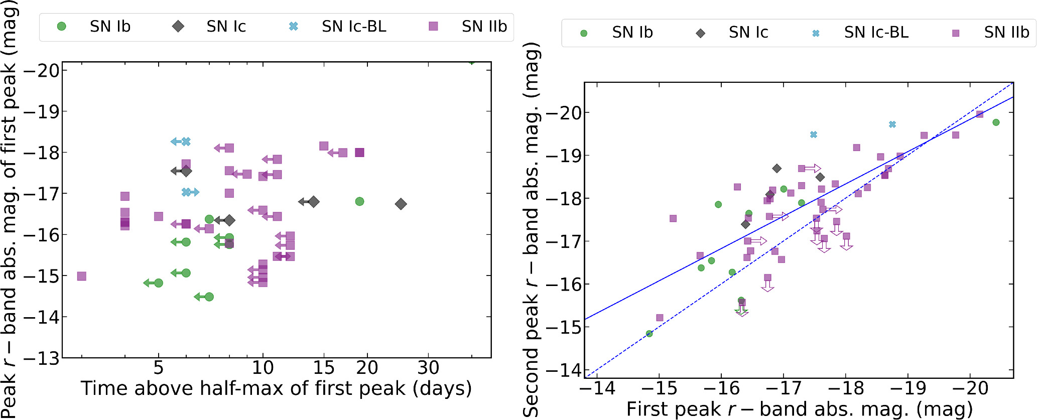
Figure 1. Left: parameter space of peak magnitude of the first peak vs. time above half-maximum of the first peak  for all double-peaked SNe observed by ZTF as part of the BTS and the CLU survey. The Type Ibc(BL) SNe in the figure are part of the sample in this work. Right: we see a correlation in the peak magnitude of the first and second peaks of the SNe following M2 = 0.8 × M1–4.7. M1 and M2 are the peak magnitudes of the first and second peak, respectively. The solid line shows the best-fit linear relation. We can infer from the y = x dashed line that the second peak is brighter than the first peak for most sources. The correlation could imply that the SNe that show double-peaked lightcurves have He-star progenitors that shed their envelope in binary interactions.
Download figure:
Standard image High-resolution imageIn Figure 2, we look at the interaction times for some SESNe where interactions were observed (Brethauer et al. 2022). We note that our sample shows interaction at earlier times compared with CSM interaction signatures for most SESNe in the literature.
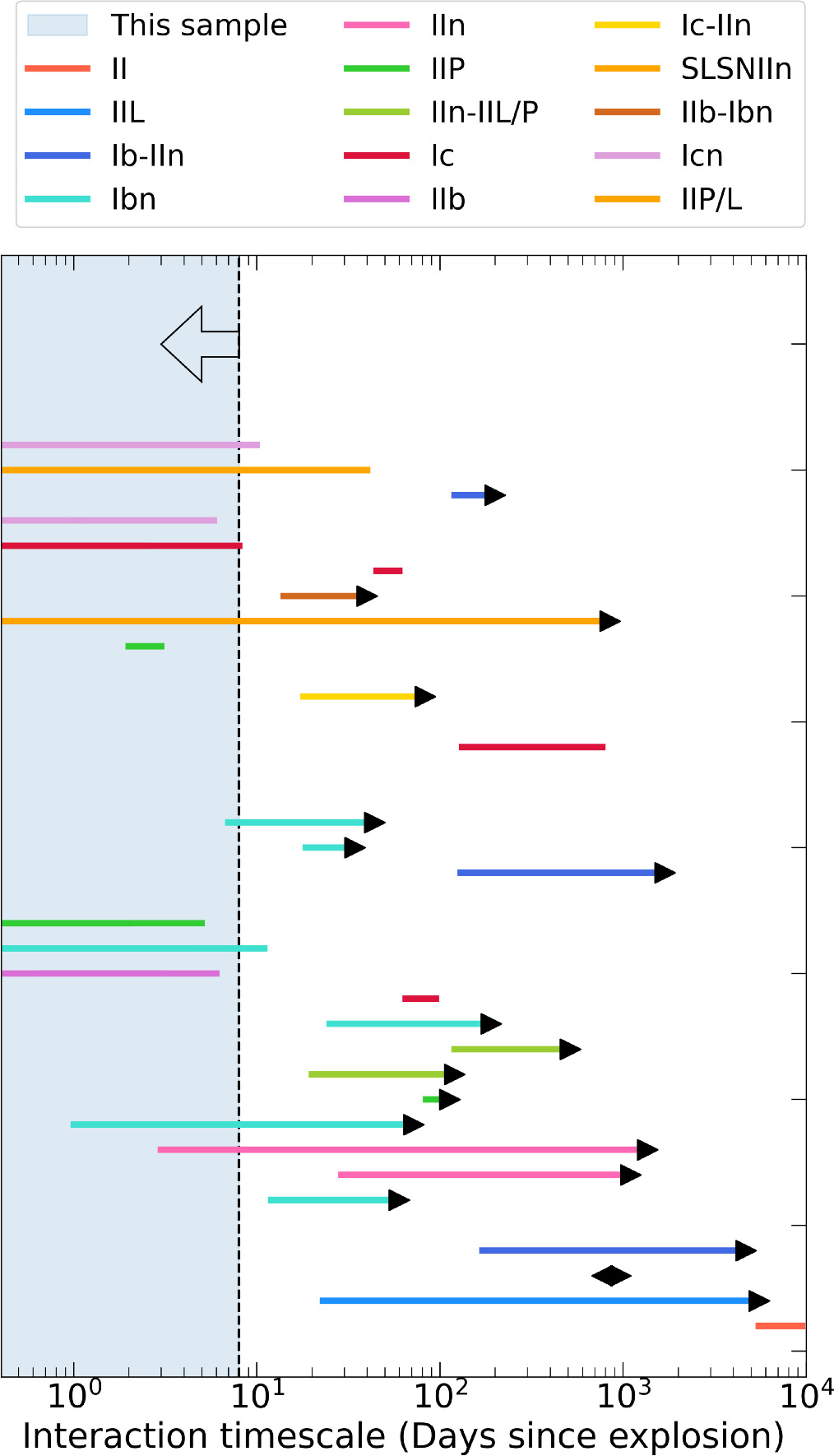
Figure 2. The interaction timescale for various SNe in the literature (from data compiled in Brethauer et al. 2022) showing signatures of CSM interaction including SNe Ibc, Ibn, and Icn are shown by the colored lines. The blue shaded region shows the range of timescale of the first peak for our sample consistent with shock-cooling ( < 8 days).
Download figure:
Standard image High-resolution image3. Data
In this section, we describe the photometric and spectroscopic data used.
3.1. Optical Photometry
We utilize forced-photometry data from the ZTF in the g, r, and i bands and from the Asteroid Terrestrial-impact Last Alert System (ATLAS; Tonry et al. 2018; Smith et al. 2020) in the c and o bands. In addition, photometry data are obtained from the Palomar 60 inch telescope (P60; Cenko et al. 2006), the Sinistro imager on the 1 m class and the Spectral imager on the 2 m class telescopes operated by Las Cumbres Observatory (Brown et al. 2013), and the Liverpool Telescope (LT; Steele et al. 2004) in the g, r, and i bands. We also obtain u-, i-, and z-band photometry for a few sources from the LT. P60 and LT data were processed using the FPipe (Fremling et al. 2016) image subtraction pipeline with Sloan Digital Sky Survey (Ahn et al. 2012) and PanSTARRS (Chambers et al. 2016) reference images. Additionally, we have early-time UV data for some sources acquired from the Ultra-violet Optical Telescope (UVOT; Roming et al. 2005), which is deployed on the Neil Gehrels Swift Observatory (Gehrels et al. 2004). UVOT data are reduced using HEAsoft. 25 The photometry data can be found in Appendix A. Figure 3 shows the lightcurve of SN 2021gno as an example. We compare the r-band absolute magnitude of the SN with our sample in Figure 4. Similar plots for the other SNe can be found in Appendix B. Figure 5 shows the lightcurves of all the SNe.
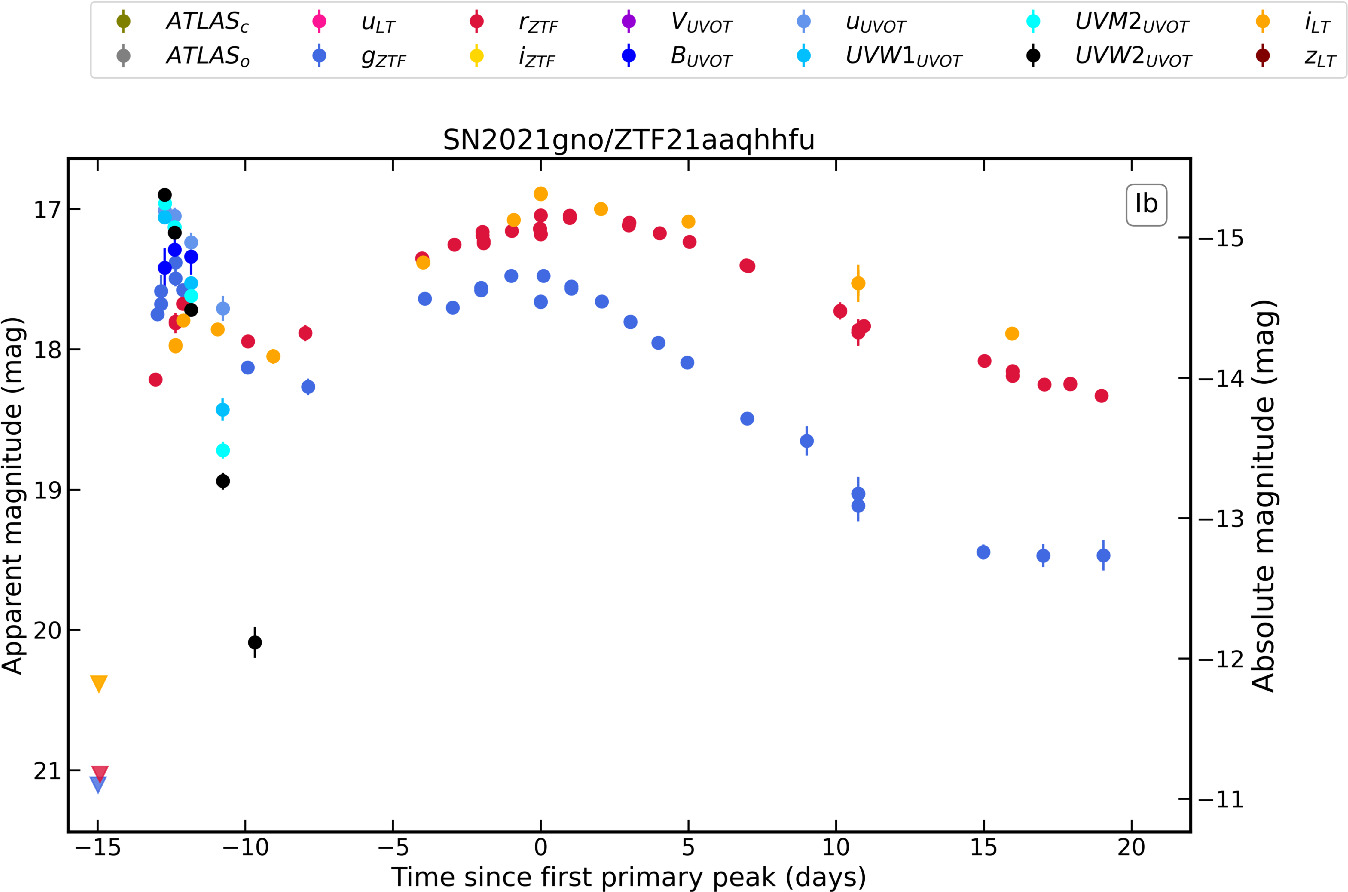
Figure 3. Lightcurve of SN 2021gno (E(B − V)MW = 0.01). The lightcurves of the other SNe can be found in Appendix B.
Download figure:
Standard image High-resolution image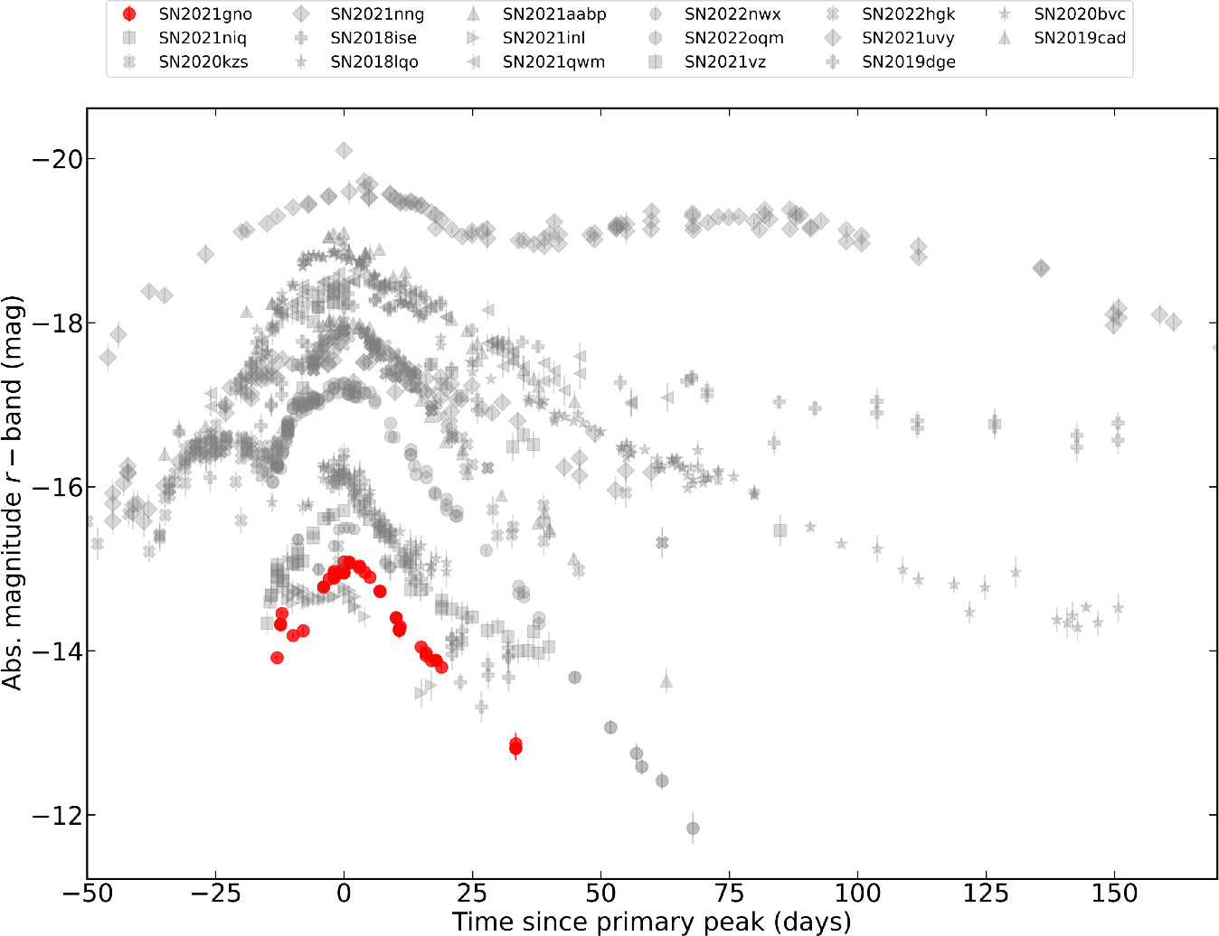
Figure 4. Comparison of the r-band absolute magnitude lightcurve of SN 2021gno to the other sources in the sample. The comparison for the other sources can be found in Appendix B.
Download figure:
Standard image High-resolution image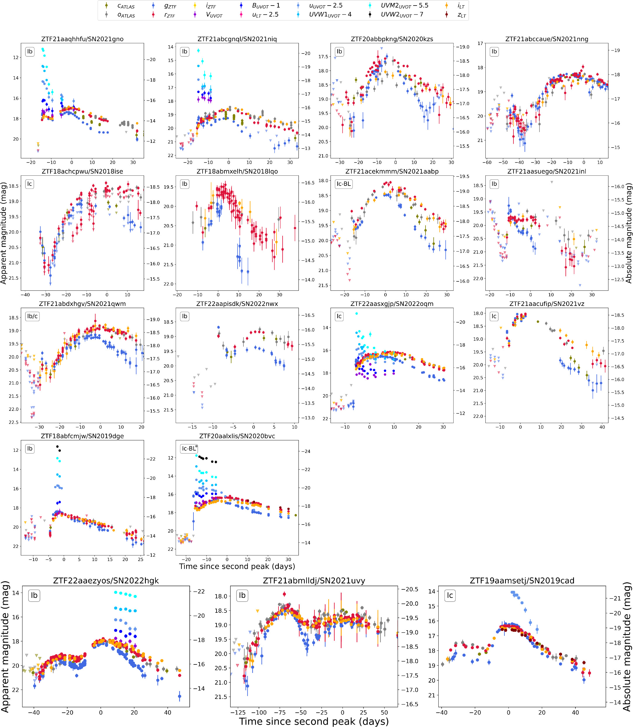
Figure 5. Top: lightcurves of double-peaked Type Ibc SNe in our sample, obtained through forced photometry from ZTF and ATLAS and follow-up observations from various instruments. Further details on the photometry can be found in Section 3.1. The left y-axis represents the apparent magnitude, while the right y-axis shows the absolute magnitude. The absolute magnitude measurements assume Milky Way and host extinction values from Table 1. The x-axis shows the number of rest-frame days since the epoch of the second peak. Bottom: the three SNe in the bottom row have an unusually long first peak with  days. We leave the detailed lightcurve analysis of these SNe for future work.
Download figure:
Standard image High-resolution image3.2. Optical Spectroscopy
We acquired spectroscopy at multiple epochs for the SNe in our sample, covering a range from 1 day to over 300 days after explosion. Each transient typically has at least one spectrum near peak luminosity for initial classification, and additional spectral follow-up was conducted as part of the ZTF surveys. Our primary classification instruments are the Spectral Energy Distribution Machine (SEDM; Blagorodnova et al. 2018) on the P60 telescope and the Double Beam Spectrograph (DBSP; Oke & Gunn 1982) on the Palomar 200 inch (P200) telescope. The DBSP spectra are reduced using the reduction pipelines described in Bellm & Sesar (2016) and Roberson et al. (2022). The SEDM data are reduced using the pipeline detailed in Rigault et al. (2019). Additionally, we obtained spectra from the Alhambra Faint Object Spectrograph and Camera on the Nordic Optical Telescope (NOT; Djupvik & Andersen 2010) and the Spectrograph for the Rapid Acquisition of Transients (SPRAT; Piascik et al. 2014). The NOT data were reduced using the PyNOT 26 and PypeIt (Prochaska et al. 2020) reduction pipelines, while we use the FrodoSpec pipeline (Barnsley et al. 2012) for reduction of SPRAT data. We obtain late-time nebular-phase spectra with the Low-Resolution Imaging Spectrometer (LRIS; Oke et al. 1995) on the Keck I telescope, with data reduced using the automated lpipe (Perley 2019) pipeline. The log of the observed spectra can be found in Table 12. Figure 6 shows the spectral sequence for SN 2021gno as an example. The spectral sequences of all the sources can be found in Appendix C.
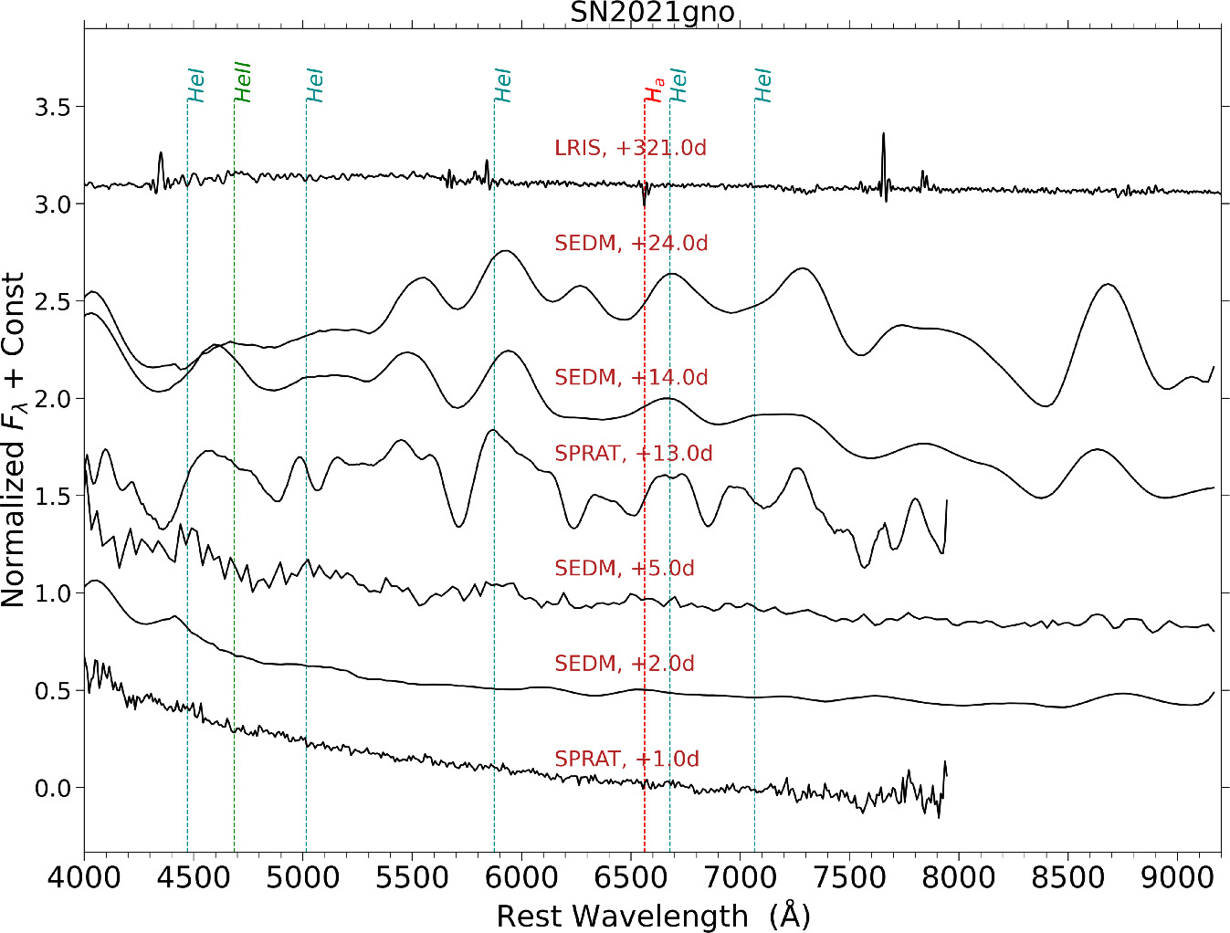
Figure 6. Spectral sequence for SN 2021gno (Type Ib) taken as part of the ZTF and CLU surveys. See Section 4.2 for details on the spectra obtained. Spectral sequences for the other sources can be found in Appendix C.
Download figure:
Standard image High-resolution image4. Methods and Analysis
4.1. Extinction Correction
For precise estimation of the luminosity and explosion properties of an SN, it is essential to determine the impact of dust extinction along the observer’s line of sight. Extinction is commonly divided into two components: the first component represents dust extinction from the Milky Way, while the second component accounts for extinction originating from the SN’s host galaxy. To correct for Galactic extinction, we employ the reddening maps provided by Schlafly & Finkbeiner (2011). For reddening corrections, we use the extinction law described by Cardelli et al. (1989) with a value of RV = 3.1.
To estimate the host galaxy extinction, we measure the equivalent width (EW) of the Na i D absorption feature (Poznanski 2013). We measure an EWNa i D of 1.5 Å, 5.5 Å, and 0.8 Å for SN 2019cad, SN 2020nng, and SN 2021nng, respectively. We do not see Na i D absorption for the other sources in the high signal-to-noise spectra. Thus, we assume zero host extinction for the rest of the sources in our analysis. To compute AV from the EW measurements, we use ![${A}_{{\rm{V}}}^{\mathrm{host}}[\mathrm{mag}]=0.78\times {\mathrm{EW}}_{\mathrm{Na}\ {\rm{I}}\ {\rm{D}}}[{\rm{\mathring{\rm A} }}]$](https://content.cld.iop.org/journals/0004-637X/972/1/91/revision2/apjad595fieqn8.gif) (Stritzinger et al. 2018). We measure
(Stritzinger et al. 2018). We measure  = 1.2 mag for SN 2019cad and
  = 0.6 mag for SN 2021nng. However, the empirical relation in Stritzinger et al. (2018) is not valid for the high EWNa i D measured for SN 2020kzs. Instead, we use the difference in the average color (g − r) of SN 2020kzs with the color expected for typical SNe Ib with no host extinction assuming the intrinsic template for Type Ib SNe provided in Stritzinger et al. (2018). Based on this, we measure
  = 1.1 mag for SN 2020kzs.
4.2. Measuring Velocity in Photospheric Spectra
As described in Section 3.2, we obtain spectra soon after explosion for all sources. We use the SuperNova Identification (SNID; Blondin & Tonry 2007) code for the classifications. For spectra contaminated by the host galaxy, we utilized the superfit (Howell et al. 2005) code for classification. The final classification as Type Ibc SNe was determined through manual inspection of the emission and absorption lines and the best-fit templates matched from SNID or superfit.
We measure the expansion velocities of the He i λ5876 and O i λ7774 lines from the absorption part of the P Cygni profiles of the spectral lines. To do this, we fit a polynomial function, whose degree is manually tuned for each spectrum (typically three), to the minima of the P Cygni profiles. These minima serve as estimates for the expansion velocity. In cases where the spectrum is dominated by galaxy lines or has low resolution, we manually inspect the spectrum to determine the minima of the absorption feature. The measured velocities are documented in Table 12. We adopt a Monte Carlo approach to estimate the uncertainties in our velocity measurements. We generate a noise spectrum by subtracting a heavily smoothed version of the spectrum from the original spectrum. The standard deviation of this noise spectrum provides an estimate of the noise of the spectrum. Next, we create simulated noisy spectra by adding noise from a standard Gaussian distribution with the calculated standard deviation. We then add these simulated spectra with the heavily smoothed spectra and recalculate the velocities. The 1σ uncertainty in the velocity measurements across all the simulated spectra is considered as the standard deviation. Fremling et al. (2018) analyzed the spectra of a sample of 45 Type Ib SNe, 56 Type Ic SNe, 17 Type Ib/c SNe, and 55 Type IIb SNe discovered by the Palomar Transient Factory (PTF) and intermediate PTF (iPTF) surveys. We compare our measured velocities with those from Fremling et al. (2018). From Figure 7, we find that the expansion velocities of the He i λ5876 and O i λ7774 lines are consistent with those of canonical Type Ibc SNe.
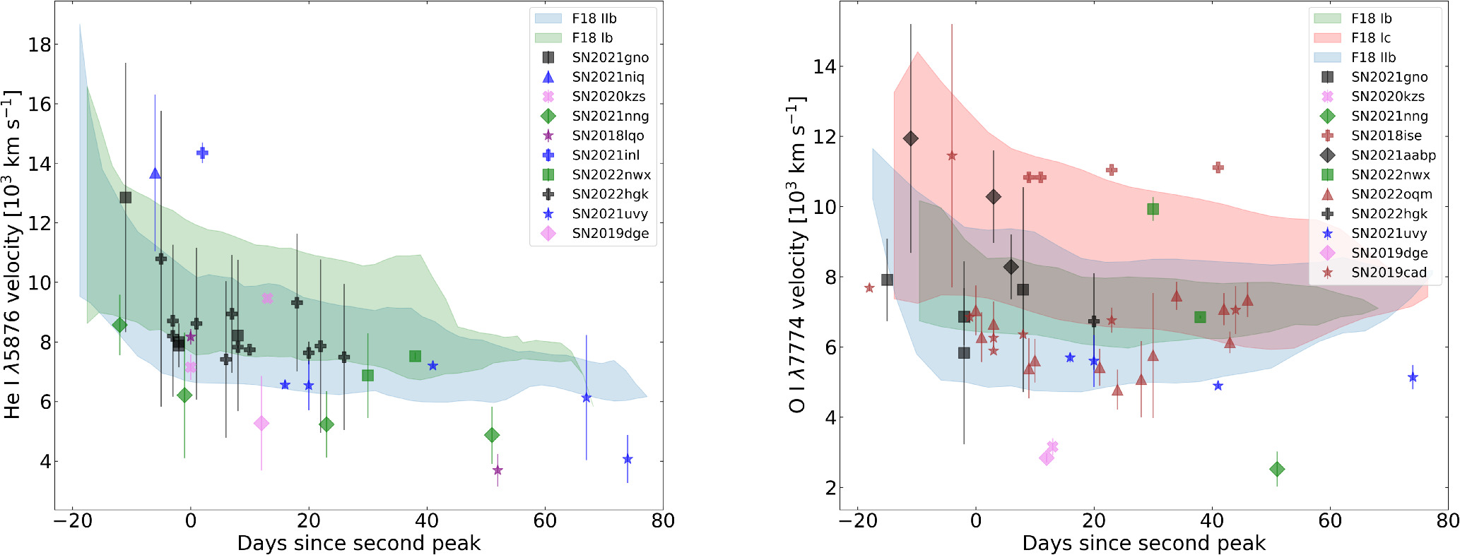
Figure 7. Left: the filled shapes represent the expansion velocity of the He i λ5876 line for each SN in our sample. The blue shaded region indicates the 1σ range of the ejecta velocities calculated for a sample of canonical Type IIb and Type Ibc SNe from Fremling et al. (2018). Right: the filled shapes represent the expansion velocity of the O i λ7774 line for each SN in our sample. Again, the blue shaded region represents the 1σ range of the ejecta velocities calculated for a sample of normal Type IIb and Type Ibc SNe from Fremling et al. (2018).
Download figure:
Standard image High-resolution image4.3. Measuring Oxygen Line Flux in Nebular Spectra
We obtained nebular-phase spectra for 10 sources with Keck and P200. A few of the nebular spectra for SN 2021gno and SN 2021inl were taken from Jacobson-Galán et al. (2022b) as noted in Table 3. We use interpolated late-time photometry to flux calibrate our nebular spectra. When late-time photometry is not available, we extrapolate the lightcurve by assuming a late-time (>30 days) i-band decline rate of 0.019 ± 0.004 mag day−1, based on the average late-time decay of the SESNe tabulated in Wheeler et al. (2015). For each spectrum, we manually set the wavelength regions and measure the line fluxes using trapezoidal integration. Uncertainties in this method are estimated by Monte Carlo sampling of the estimated fluxes by adding noise (scaled to nearby regions of the continuum) to the line profile. Table 3 presents the measured fluxes of [Ca ii] λ λ7291, 7324 and [O i] λ λ6300, 6364, along with their flux ratio.
Table 3. Summary of the Nebular Properties
| Source | Spectra Tel.+Inst. | Phase | [Ca ii]/[O i] Flux Ratio | [O i] Lum. | O Mass |
|---|---|---|---|---|---|
| (days since primary peak) | (1038 erg s−1) | (M⊙) | |||
| ZTF21aaqhhfu/SN 2021gno a | Keck + LRIS | 84 | 8.97 ± 1.79 | 3.9 ± 0.4 | 0.1−0.3 |
| ZTF18achcpwu/SN 2018ise | Keck + LRIS | 120 | 0.93 ± 0.08 | 303.45 ± 12.11 | 7.5−20.0 |
| ZTF18abmxelh/SN 2018lqo | Keck + LRIS | 52 | >50 | <1.6 | <0.1 |
| ZTF21aasuego/SN 2021inl a | Keck + LRIS | 111 | 4.39 ± 0.88 | 8.2 ± 0.4 | 0.2−0.6 |
| ZTF22aapisdk/SN 2022nwx | Keck + LRIS | 86 | 10.95 ± 1.15 | 7.62 ± 0.90 | 0.2−0.5 |
| ZTF22aasxgjp/SN 2022oqm | P200 + DBSP | 74 | >22 | <0.17 | <0.01 |
| ZTF22aaezyos/SN 2022hgk | Keck + LRIS | 75 | 1.13 ± 0.04 | 104 ± 1.4 | 2.6−7.4 |
| ZTF21abmlldj/SN 2021uvy | Keck + LRIS | 426 | 3.38 ± 0.15 | 81 ± 8 | 0.6−3.1 |
| ZTF18abfcmjw/SN 2019dge | Keck + LRIS | 83 | 1.22 ± 0.19 | 2.44 ± 0.33 | 0.06−0.1 |
Note.
a From Jacobson-Galán et al. (2022b).Download table as: ASCIITypeset image
4.4. Modeling Lightcurves
4.4.1. Blackbody Fit
We estimate the bolometric lightcurve for epochs where we have detections in at least two filters by fitting a blackbody function. For each epoch, we use a Python emcee package (Foreman-Mackey et al. 2013) to perform a Markov Chain Monte Carlo analysis in order to estimate the blackbody temperature (TBB), radius (RBB), and luminosity (LBB). The uncertainties of the model parameters are determined by extracting the 16th and 84th percentiles of the posterior probability distribution. We note that UV coverage is only available for SNe 2020bvc, 2022oqm, and 2021gno. For these three SNe, the blackbody fit is done on the available UV−optical photometry. For the rest, the blackbody fit is done on the available optical photometry only. The best-fit parameters can be found in Appendix D.
4.4.2. Fitting Shock Cooling in First Peak
In our sample, all sources exhibit a lightcurve characterized by two distinct peaks. The rapid rise of the first peak, accompanied by an initial blue color and high temperature, indicates that the first peak is likely dominated by cooling emissions from the shock-heated extended envelope (Nakar & Piro 2014; Piro 2015). We plot the peak luminosity versus time above half-maximum in Figure 1. The same is shown for the first peak of all double-peaked Type IIb SNe (not part of the sample in this work) from BTS+CLU. We note that 43 out of 193 Type IIb SNe had detections of two peaks (K. K. Das et al. 2024, in preparation). In the right panel of Figure 1, we plot the peak r-band magnitude of the first peak versus the peak r-band magnitude of the second peak. For the first time, we find that a correlation exists between the peak magnitudes of the first and the second peak. The Pearson correlation coefficient is 0.79 (p < 10−5). A similar correlation is also seen for the g band, with a Pearson correlation coefficient of 0.81 (p < 10−5). The physical reason for this correlation is not clear. The first-peak brightness is primarily dependent on the radius of the progenitor, while the peak of the second peak is primarily dependent on the Ni mass. The correlation could imply that the SNe that show double-peaked lightcurves come from He-star progenitors that shed their envelope in binary interactions. Then, this correlation could be related to the He main sequence (see Figure 5 in Sravan et al. 2020), with the progenitor radius being related to the effective temperature and the Ni mass being related to the luminosity. This would require that the Ni mass is correlated with the ejecta mass (Lyman et al. 2016). This assumes that SESNe come from He stars. Such a correlation could also exist if the first peak is also powered by nickel. This is possible if nickel is not entirely in the core but is also present in the outer envelope. However, it is unlikely that this trace amount of nickel can make a significant contribution to the early luminosity. We note that our survey is biased against sources that have a very faint first-peak luminosity.
It is important to note that some of the SNe in our sample do not have well-sampled first peaks in both the rising and fading phases. To fit the multiband photometry in the shock-cooling phase, we use the model proposed by Piro et al. (2021). This model allows us to determine key parameters, such as the explosion time (texp), extended material mass (Mext), radius (Rext), and energy (Eext). We use the Python emcee package (Foreman-Mackey et al. 2013) to perform a multiband photometry data fitting analysis. We add a systematic error of 50% to account for uncertainties in the density and opacity assumptions used in the model. Table 4 and Appendix E provide the best-fit values and corresponding fits for each SN.
Table 4. Shock-cooling Modeling
| Source | Eext | Rext | Mext | texp |
|---|---|---|---|---|
| (×1049 erg) | R⊙ | (×10−2 M⊙) | JD | |
| ZTF21aaqhhfu/SN 2021gno |

|

|

|

|
| ZTF21abcgnql/SN 2021niq |

|

|

|

|
| ZTF20abbpkng/SN 2020kzs |

|

|

|

|
| ZTF21abccaue/SN 2021nng |

|

|

|

|
| ZTF18achcpwu/SN 2018ise |

|

|

|

|
| ZTF18abmxelh/SN 2018lqo |

|

|

|

|
| ZTF21acekmmm/SN 2021aabp |

|

|

|

|
| ZTF21aasuego/SN 2021inl |

|

|

|

|
| ZTF21abdxhgv/SN 2021qwm |

|

|

|

|
| ZTF22aapisdk/SN 2022nwx |

|

|

|

|
| ZTF22aasxgjp/SN 2022oqm |

|

|

|

|
| ZTF21aacufip/SN 2021vz |

|

|

|

|
| ZTF18abfcmjw/SN 2019dge |

|

|

|

|
| ZTF20aalxlis/SN 2020bvc |

|

|

|

|
Download table as: ASCIITypeset image
In Figure 8, we compare the best-fit parameters with those for some H-poor SNe for which CSM interactions were detected. These CSM radii cover a wide range of distances from the explosion site, from ∼3 × 10¹³ to 1018 cm. The range of inferred CSM masses is also broad, spanning from ∼10−4 M⊙ up to tens of M⊙ of material (Figure 8). We note that the physical parameters have been estimated with a variety of observational “tracers.”
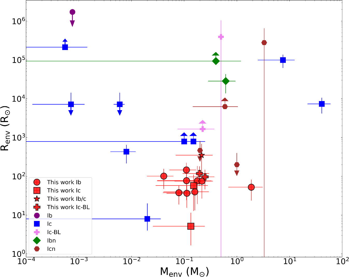
Figure 8. Comparison of the CSM parameters of the sample in this paper with the CSM properties of other SNe in the literature (from Brethauer et al. 2022). We note that the physical parameters have been estimated with a variety of observational “tracers” and hence probe different regions of the CSM.
Download figure:
Standard image High-resolution image4.4.3. Shock-cooling Order-of-magnitude Limits for the First Peak
We make the assumption that the layer going through shock cooling has a radius Rext and mass Mext. The expansion timescale is  , where vext is the velocity of this layer. Photons undergo diffusion from this layer within a timescale approximately given by tdiff ∼ τ
Rext/c. The bulk of the photons emerge from the layer where
, where vext is the velocity of this layer. Photons undergo diffusion from this layer within a timescale approximately given by tdiff ∼ τ
Rext/c. The bulk of the photons emerge from the layer where  or τ ∼ c/vext.
We assume ρ ∼ Mext/(4π
R3/3). At a specific radius, the optical depth τ decreases as a result of expansion: τ ∼ κ
ρ
R. The radius increases as R ∼ vext
t, so  . Setting this equal to c/vext,

We have an upper limit on the time to peak of tp as the epoch of the first peak calculated from the analytical model described in the previous section. We take κ = 0.2 cm2 g−1 for a hydrogen-poor gas and vext ∼ 0.1c. Altogether, we find Mext ∼ 0.01–1 M⊙. Note that the predicted values are upper limits because the rise time was likely faster than our measurements. The limits are listed in Table 5. The values obtained from the analytical model described in the previous section are consistent with the limits obtained.
Table 5. Order-of-magnitude Shock-cooling CSM Estimates
| Source | MCSM | RCSM |
|---|---|---|
| (M⊙) | (R⊙) | |
| SN 2021gno | 0.02 | 10 |
| SN 2021niq | 0.20 | 10 |
| SN 2020kzs | 0.53 | 20 |
| SN 2021nng | 0.06 | 40 |
| SN 2018ise | 0.05 | 60 |
| SN 2018lqo | 1.23 | 10 |
| SN 2021aabp | 0.34 | 60 |
| SN 2021inl | 0.04 | 10 |
| SN 2021qwm | 0.07 | 220 |
| SN 2022nwx | 0.03 | 10 |
| SN 2022oqm | 0.01 | 30 |
| SN 2021vz | 0.28 | 1030 |
| SN 2022hgk | 0.18 | 20 |
| SN 2021uvy | 11.31 | 260 |
| SN 2019dge | 0.06 | 30 |
| SN 2020bvc | 0.01 | 210 |
| SN 2019cad | 0.86 | 20 |
Download table as: ASCIITypeset image
Next, we estimate the radius Rext. If the shock deposits energy Edep into the layer, which then cools from expansion, we can estimate the energy Ecool ∼ Edep(Rext/vext
t). Thus, the luminosity from cooling is Lcool ∼ Edep
Rext/vext
t2. We assume that the deposited energy is half the kinetic energy EKE of the shock,  , where ρ and dR are the density and width of the layer. Taking
  and dR ≈ Rext, we find

Taking the above Mext, tp values, vext = 0.1c, and lower limits on the peak luminosity from the bolometric blackbody fits, we find Rext in the range ≈10–200 R⊙. We can only measure a lower limit on the radius because the true peak luminosity is likely higher than what we can measure.
The limits are listed in Table 5. The values obtained from the analytical model described in the previous section are consistent with the limits obtained.
4.4.4. Ruling Out Shock Breakout from CSM for the First Peak
In this section, we conduct a rough estimation to determine if the rise time and peak luminosity can be accounted for by a model in which shock interaction powers the lightcurve (“wind shock breakout”).
The shock-crossing timescale is tcross ∼ RCSM/vs , which is ∼0.01 day, assuming a shock velocity (vs ≈ 0.1c) for the observed radius range, which is around 2 orders of magnitude less than the observed timescale. The estimated limits are listed in Table 6.
Table 6. Order-of-magnitude Shock-breakout CSM Estimates
| Source | MCSM | RCSM |
|---|---|---|
| (10−3 M⊙) | (R⊙) | |
| SN 2021gno | 0.19 | 5900 |
| SN 2021niq | 0.11 | 19,400 |
| SN 2020kzs | 0.13 | 3100 |
| SN 2021nng | 0.69 | 10,800 |
| SN 2018ise | 1.13 | 9400 |
| SN 2018lqo | 0.03 | 47,400 |
| SN 2021aabp | 0.40 | 25,000 |
| SN 2021inl | 0.15 | 8900 |
| SN 2021qwm | 3.45 | 11,300 |
| SN 2022nwx | 0.22 | 6800 |
| SN 2022oqm | 1.26 | 4700 |
| SN 2021vz | 8.12 | 22,500 |
| SN 2022hgk | 0.15 | 18,500 |
| SN 2021uvy | 0.31 | 143,700 |
| SN 2019dge | 0.53 | 10,800 |
| SN 2020bvc | 7.26 | 5000 |
| SN 2019cad | 0.1 | 39,500 |
Download table as: ASCIITypeset image
The shock heats the CSM with an energy density that is roughly half of the kinetic energy of the shock, so the energy density of the CSM  . The luminosity is the total energy deposited divided by tcross,

which is >1044 erg, again a few orders higher than the observations, assuming a constant density.
Therefore, considering shock velocities (0.1c) comparable to the observed expansion of the photospheric radius, Table 6 indicates that we would require higher values for MCSM than what is expected for unbound CSM. Thus, we rule this out as a possible explanation for the early bump.
4.4.5. Modeling the Radioactively Powered Second Peak
In this section, we describe the modeling of the second peak of the SNe. First, we estimate the contribution of the cooling emission to the bolometric luminosity using the best-fit parameters obtained in Section 4.4.2. This cooling component is then subtracted from the bolometric lightcurves obtained through blackbody fitting. We employ two methods to fit the peak, assuming it is powered by radioactive decay. First, we apply the analytical model outlined in Arnett et al. (1989), Valenti et al. (2008), and Wheeler et al. (2015). Using this model, we constrain the characteristic photon diffusion timescale (τm ), characteristic γ-ray diffusion timescale (to ), and nickel mass (MNi). Additionally, we use relations from Wheeler et al. (2015) that provide the kinetic energy in the ejecta (Ekin) and the ejecta mass (Mej) as functions of photospheric velocity (vph) and (τm ). We use the vph measured using the average He i line and O i velocity from the photospheric spectra within 5 days of the second-peak epoch for Type Ib and Type Ic(BL) SNe, respectively, listed in Section 4.2. If there are no velocity measurements available from spectra within 5 days of the second peak, we assume an average velocity of 8000 km s−1. For SN 2020bvc, we use vph = 18,000 km s−1 derived in Ho et al. (2020). Second, we use the lightcurve analytical models given in Khatami & Kasen (2019) to estimate the various explosion parameters. Further details on the model fitting can be found in Yao et al. (2020, their Appendix B). Figure 9 shows the parameter space occupied by these transients with ejecta mass varying from ≈0.2 to 7 M⊙ and nickel mass varying from 0.01 to 0.5 M⊙. For SN 2021inl, we note that the estimated ejecta mass and kinetic energy values are higher than those estimated in Jacobson-Galán et al. (2022b), as they used a lower photospheric velocity of 7500 km s−1, instead of the 14,350 km s−1 used in this work. We compare the ejecta mass and nickel mass with those from Taddia et al. (2018) in Figure 9. The best-fit parameters and fits are provided in Table 7 and Appendix F.
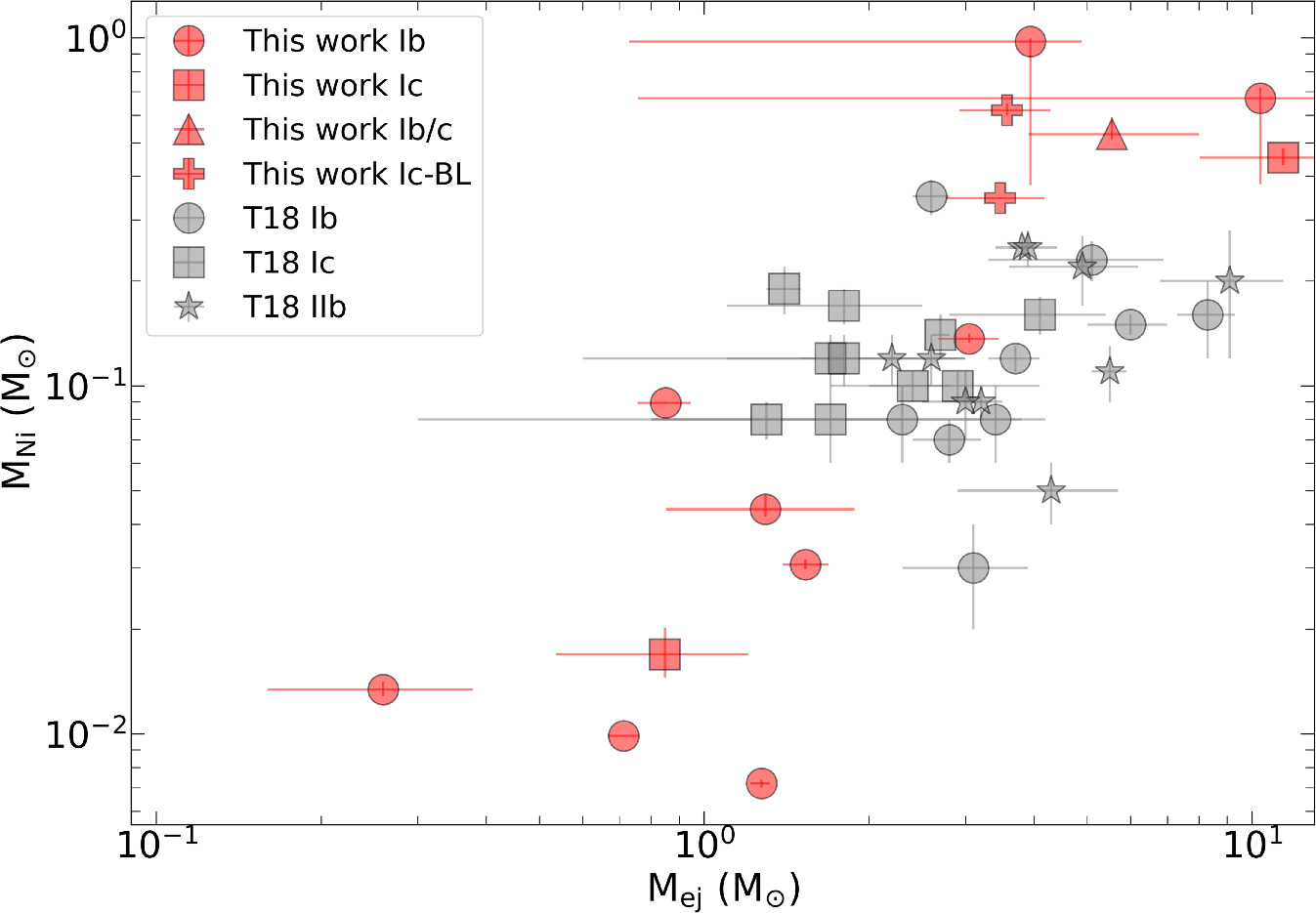
Figure 9. The distribution of measured 56Ni mass vs. ejecta mass for SNe in this sample compared to normal Type Ibc and IIb SNe from Taddia et al. (2018).
Download figure:
Standard image High-resolution imageTable 7. Summary of the Best-fit Physical Parameters Obtained by Radioactive Decay Modeling of the Second Peak of the SNe in Our Sample
| Source | MNi−Ar | MNi−KK | τm | Velocity | Mej−Ar | Mej−KK | Ekin | t0 |
|---|---|---|---|---|---|---|---|---|
| (0.01 M☉) | (0.01 M☉) | (days) | (km s−1) | (M☉) | (M☉) | (1051 erg) | (days) | |
| SN 2021gno |

| 1.09 |

| 7940.0 ± 500.0 |

| 0.53 |

|

|
| SN 2021niq |

| 5.20 |

| 8000 ± 1600.0 |

| 0.88 |

|

|
| SN 2020kzs |

| 18.31 |

| 7150.0 ± 430.0 |

| 1.68 |

|

|
| SN 2021nng |

| 72.17 |

| 6210.0 ± 2110.0 |

| 2.85 |

|

|
| SN 2018ise |

| 100.36 |

| 8000 ± 1600.0 |

| 6.05 |

|

|
| SN 2018lqo |

| 3.61 |

| 8170.0 ± 260.0 |

| 0.99 |

|

|
| SN 2021aabp |

| 76.66 |

| 10,280.0 ± 1320.0 |

| 1.95 |

|

|
| SN 2021inl |

| 0.77 |

| 14,350.0 ± 350.0 |

| 0.91 |

|

|
| SN 2021qwm |

| 82.22 |

| 8000 ± 1600.0 |

| 2.92 |

|

|
| SN 2022nwx |

| 1.16 |

| 8000 ± 1600.0 |

| 0.36 |

|

|
| SN 2022oqm |

| 10.18 |

| 6660.0 ± 690.0 |

| 0.60 |

|

|
| SN 2021vz |

| 34.23 |

| 8000 ± 1600.0 |

| 0.68 |

|

|
| SN 2019dge |

| 1.40 |

| 8000 ± 1600.0 |

| 0.23 |

|

|
| SN 2020bvc |

| 40.44 |

| 18,000 ± 3600.0 |

| 2.18 |

|

|
Note. The “Ar” subscript refers to the Arnett et al. (1989) model, while the “KK” subscript refers to the Khatami & Kasen (2019) model. The photospheric velocity is estimated as described in Section 4.4.5.
Download table as: ASCIITypeset image
5. Constraining Progenitor Mass
The late-time evolution of a star, including pre-SN mass loss, is strongly dependent on the progenitor mass. In this section, we try to provide rough estimates of the progenitor mass based on the nebular spectra and the lightcurves.
We have at least one nebular spectrum for 10 SNe obtained using LRIS on the Keck I telescope. Using the procedure described in Section 4.3, we calculate the [Ca ii] λ λ7291, 7324 to [O i] λ λ6300, 6364 flux ratio and determine the [O i] λ λ6300, 6364 fluxes (Table 3). Next, we use these [O i] luminosity measurements to compute the oxygen abundance and, subsequently, the progenitor mass. To determine the minimum required oxygen mass for a given [O i] luminosity, we use the analytical relation in Uomoto (1986). This analytical formula is applicable where the electron density is higher than ∼7 × 105 cm−3. This is estimated to be valid for our case, with ejecta mass in the range of 0.3–6 M☉. We use temperature values of ≈3500–4000 K estimated in other CCSNe from the [O i] emission (Sollerman et al. 1998; Elmhamdi 2011). Using this, we get an estimate of the O mass in our sample in the range of ≈0.001–1 M⊙ (see Table 3).
We use these O mass estimates to constrain the progenitor mass. To achieve this, we refer to the work of Dessart et al. (2021), who conducted 1D nonlocal thermodynamic equilibrium radiative transfer calculations specifically for nebular-phase stripped SNe. Strong [Ca ii] and weak [O i] emission is predicted for lower-mass He stars. The high [Ca ii]/[O i] flux ratio we observe for SNe 2021gno, 2021inl, 2022nwx, 2022oqm, and 2018lqo in our sample is indicative of a low initial He-star mass progenitor. In Figure 10, we present a comparison of the measured O mass in our sample and the synthesized O mass obtained from He-star progenitor models from both binary evolution (Dessart et al. 2021) and single-star models (Sukhbold et al. 2016). Of the 14 SNe consistent with shock cooling, we find that the SNe with progenitor mass less than 12 M⊙ are SNe 2019dge, 2021gno, 2021inl, 2022nwx, 2022oqm, and 2018lqo. To determine the progenitor mass from the He-star mass, we use the relation provided in Woosley & Heger (2015).
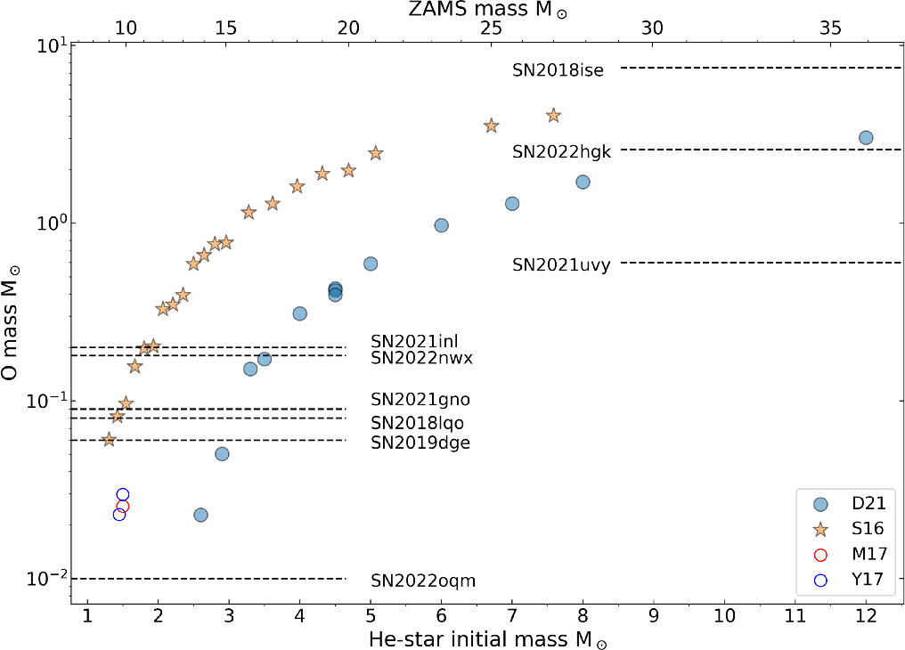
Figure 10. The O mass measurements are depicted by horizontal dashed lines. The O yields from the He-star progenitor models, assuming binary evolution (Dessart et al. 2021), are represented by filled blue dots. The O yields from the single-star models (Sukhbold et al. 2016) are indicated by filled orange stars. Additionally, we show the O mass predictions from nucleosynthetic models of lower ZAMS stars from USSNe models by Moriya et al. (2017) and Yoshida et al. (2017).
Download figure:
Standard image High-resolution imageIn order to make a comparison with such low progenitor masses, we also consider estimates of the O synthesized in the case of USSNe. USSNe arise from low-mass He stars (<3.5 M⊙) that have been highly stripped by a binary companion in a close orbit, leaving behind CO cores with approximate masses ranging from 1.45 to 1.6 M⊙ at the time of the explosion (Tauris et al. 2015). It is worth noting that the CO core mass serves as a reliable indicator of the zero-age main-sequence (ZAMS) mass, as it remains unaffected by binary stripping (Fransson & Chevalier 1989; Jerkstrand et al. 2014, 2015). We find that the O yields for the CO cores of USSNe are higher than five SNe in our sample (see Figure 10).
We caution that these measurements assume that the radioactive energy deposited in the O-rich shells is primarily released through cooling in the [O i] lines. However, the presence of impurity species can affect the [O i] luminosities. For example, Dessart & Hillier (2020) showed that if Ca is mixed into the O-rich regions, the [O i] line emissions are weakened. Nevertheless, extensive studies of CCSNe have indicated that mixing is not significant in these events. Detailed modeling of CCSNe has revealed that the [Ca ii] lines are the primary coolant in the Si-rich layers, while the emission from [O i] originates from the outer layers rich in oxygen, formed during the hydrostatic burning phase (Jerkstrand et al. 2015; Dessart & Hillier 2020). Additionally, Polin et al. (2021) have demonstrated that even a contamination of 1% level of Ca can cool a nebular region entirely through [Ca ii] emission. Thus, if these ejecta regions were mixed, it would be challenging to observe the emission of the [O i] line.
We note that the low ejecta mass (≲1.5 M⊙) for SNe 2021gno, 2021inl, 2022nwx, 2018lqo, and 2021niq is consistent with those predicted for the lower end of the He-star mass stars based on predicted ejecta properties of H-poor stars (e.g., Dessart et al. 2021). Nebular spectra estimates for all of the above SNe are also consistent with low ZAMS mass, except for SN 2021niq, for which we do not have any nebular spectra. Also, for SN 2022oqm, the ejecta mass is not consistent with the progenitor mass estimate from the nebular spectra. In this paper, we consider SN 2021gno, SN 2021niq, SN 2021inl, SN 2022nwx, SN 2018lqo, and SN 2019dge as potential SNe with progenitor masses less than ∼12 M⊙.
6. Mass-loss Scenarios
In the previous sections, we presented the results from the analysis of our double-peaked Type Ibc(BL) sample that included lightcurve and spectral properties. In this section, we try to understand the physical process that gave rise to the first peak. The early bump is most likely due to interaction with the external stellar material that is part of the extended bound envelope of a massive star or unbound material ejected in a pre-SN mass-loss event. There is other evidence for CSM interaction for some of the SNe in our sample. For example, Jacobson-Galán et al. (2022b) measured a CSM mass of 0.3–1.6 × 10⁻³ M⊙ that extends up to 5 × 1014 cm. Luminous X-ray and radio counterparts were observed for SN 2020bvc (Ho et al. 2020). Irani et al. (2024) predict the presence of C/O-rich CSM at 2–5 × 1014 cm based on early-time spectra. Similarly, early-time spectra for SN 2019dge (Yao et al. 2020) were used to constrain the distance of He-rich CSM at ≳3 × 1013 cm. The sample provides a unique opportunity to understand the origin of the CSM from late-time stellar evolution. There are different theoretical models for possible pre-SN mass loss. In this section, we explore these scenarios and compare them to the observations.
6.1. Pre-SN Mass Loss for Progenitor Masses ≲12 M⊙
6.1.1. Low-mass Binary He Stars
We know that the majority (∼70%) of young massive stars live in interacting binary systems (Mason et al. 1998; Sana et al. 2012). Recent evidence suggests that Type Ibc SNe form when less massive stars are stripped due to a binary companion (e.g., Podsiadlowski et al. 1992). These stripped stars are formed when they lose their hydrogen envelopes through case B mass transfer (MT) after hydrogen burning. The stripped stars with MHe ≲ 4 M⊙ expand again and lose a significant amount of their He envelope through case BC MT. This results in stars with low precollapse masses, which can explain the inferred Mej of the sources with low progenitor mass and low ejecta mass constraints.
There have been attempts to model the case BB mass transfer to make predictions for mass loss and the final fate of the progenitor (Yoon et al. 2010; Tauris et al. 2013, 2015; Laplace et al. 2020). However, these do not predict the significant CSM that we infer in our observations. However, Wu & Fuller (2022b) find that when the O/Ne core burning is taken into account, He stars of masses ≈2.5–3 M⊙ rapidly reexpand. As a result, they undergo high rates of binary mass transfer weeks to decades before core collapse. In part A and part B, we look at the possible cases where the shock passes through this reexpanded bound material before and after the late-time MT. In part C, we look at the possible case where the shock passes through the unbound material ejected as part of the late-time MT.
6.2. Part A: Bound Stellar Material before Late-time Binary Mass Transfer
Stripped stars with initial masses 2.5 M⊙ ≲ MHe ≲ 3 M☉ expand by 2 orders of magnitude during C burning beginning ∼105 yr before core collapse. Wu & Fuller (2022a) found that the radius can expand to ∼200 R⊙ for low-mass He stars during O/Ne burning.
We investigate if the low-luminosity first bumps we see for those with low progenitor mass are produced as the shock from the core collapse passes through this bound puffed-up stellar envelope. We can see from Table 8 that the models for single-star evolution from Wu & Fuller (2022b) can puff up to a radius that is consistent with what is calculated from the shock-cooling modeling.
Table 8. Bound Stellar Material Properties of a Single Star
| Initial Mass | Rmax | Mass 
| Mass (>5 R⊙) |
|---|---|---|---|
| (M⊙) | (R⊙) | (M⊙) | (M⊙) |
| 2.51 | 446.68 | 1.09 | 1.10 |
| 2.55 | 407.38 | 1.09 | 1.10 |
| 2.58 | 154.88 | 1.04 | 1.04 |
| 2.62 | 239.88 | 1.14 | 1.14 |
| 2.65 | 151.36 | 1.12 | 1.13 |
| 2.68 | 181.97 | 1.15 | 1.16 |
| 2.72 | 177.83 | 1.17 | 1.17 |
| 2.75 | 70.79 | 0.82 | 0.73 |
| 2.79 | 66.07 | 0.93 | 0.87 |
| 2.82 | 44.67 | 1.01 | 0.92 |
| 2.86 | 40.74 | 1.04 | 0.94 |
| 2.90 | 58.88 | 1.09 | 1.02 |
| 2.92 | 24.55 | 0.55 | 0.20 |
Download table as: ASCIITypeset image
Based on the density profiles of these stars (see Figure 15), we assume the material at r
 (Nakar & Piro 2014) is the bounded envelope responsible for the early bump, where Rmax is the radial distance of the star where the density drops below 10−7 g cm−3. We also compare the bound envelope properties of binary and single stars from Tauris et al. (2015) and Laplace et al. (2020) with those calculated for our sample in Figure 11. We find that the expected envelope mass for these models is ∼1.2 M☉, an order of magnitude greater than the observed values.
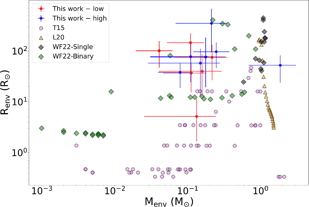
Figure 11. Comparison of the envelope parameters derived using analytical shock-cooling models as described in Section 4.4.2 (red crosses) with bound envelope properties from various binary and single-star models (WF22, Wu & Fuller 2022b; L20, Laplace et al. 2020; T15, Tauris et al. 2015). The SNe with low progenitor masses (≲12 M⊙) and higher progenitor masses are shown in red and blue, respectively.
Download figure:
Standard image High-resolution imageWe also note that the above scenario would require that the star not interact afterward with the binary companion after undergoing case B mass transfer. This is possible when the binary stars have very large periods so that the Roche lobe is not filled during the expansion. Wu & Fuller (2022b) find that the highest-mass models MHe ≥ 2.8 M⊙ with orbital period (Porb) = 100 days do not expand enough to fill their Roche lobes.
However, in these cases, it is more likely that the substantial radius expansion of the stripped stars suggests the possibility of them reoccupying their Roche lobes and experiencing subsequent phases of mass transfer (Dewi et al. 2002; Dewi & Pols 2003; Ivanova et al. 2003). Additional phases of mass transfer can produce stars with low envelope masses, possibly explaining the low ejecta mass we observe for those with low progenitor mass. We discuss this in the next part.
6.3. Part B: Bound Stellar Material after Late-time Binary Mass Transfer
Wu & Fuller (2022b) calculated the mass-loss rates from the late-time binary transfer described earlier and the accumulated mass loss at Porb = 1, 10, and 100 days. After the late-time mass transfer, the final masses range between ∼1.4 and 2.9 M⊙. As these models reach Si burning with final masses ≥1.4 M⊙, they are expected to undergo core collapse. Assuming MNS = 1.4 M⊙, the implied SN ejecta masses are ≲1.5 M⊙ The density profiles of these stars after the late-time mass transfer are shown in Appendix H. The envelope radius of most of these binary stars (especially those with Porb = 10 days) is consistent with the observed values (see Table 9 and Figure 11). Using these density profiles and the same procedure used in the previous section, we get an envelope mass range of 0.01–0.1 M⊙, which is consistent with the measured mass.
Table 9. Bound Stellar Material Properties after Binary Mass Transfer
| Initial Mass | Period | Rmax | Mass 
| Mass (>5 R⊙) |
|---|---|---|---|---|
| (M⊙) | (days) | (R⊙) | (M⊙) | (M⊙) |
| 2.51 | 100 | 79.43 | 0.00 | 0.00 |
| 2.55 | 100 | 81.28 | 0.06 | 0.05 |
| 2.58 | 100 | 407.38 | 0.22 | 0.22 |
| 2.62 | 100 | 346.74 | 0.30 | 0.30 |
| 2.65 | 100 | 109.65 | 0.44 | 0.44 |
| 2.68 | 100 | 331.13 | 0.35 | 0.36 |
| 2.72 | 100 | 199.53 | 0.69 | 0.70 |
| 2.75 | 100 | 109.65 | 0.85 | 0.85 |
| 2.51 | 10 | 15.85 | 0.01 | 0.00 |
| 2.55 | 10 | 13.18 | 0.06 | 0.02 |
| 2.58 | 10 | 12.30 | 0.06 | 0.01 |
| 2.62 | 10 | 11.75 | 0.04 | 0.00 |
| 2.65 | 10 | 12.30 | 0.11 | 0.04 |
| 2.68 | 10 | 12.30 | 0.12 | 0.05 |
| 2.72 | 10 | 12.88 | 0.16 | 0.06 |
| 2.75 | 10 | 11.48 | 0.17 | 0.05 |
| 2.79 | 10 | 11.22 | 0.21 | 0.07 |
| 2.82 | 10 | 12.02 | 0.30 | 0.10 |
| 2.86 | 10 | 13.18 | 0.40 | 0.14 |
| 2.90 | 10 | 14.13 | 0.56 | 0.25 |
| 2.92 | 10 | 15.49 | 0.60 | 0.26 |
| 2.51 | 1 | 2.69 | 0.00 | 0.00 |
| 2.55 | 1 | 3.02 | 0.00 | 0.00 |
| 2.58 | 1 | 2.51 | 0.00 | 0.00 |
| 2.62 | 1 | 2.40 | 0.00 | 0.00 |
| 2.65 | 1 | 2.45 | 0.00 | 0.00 |
| 2.68 | 1 | 2.34 | 0.01 | 0.00 |
| 2.72 | 1 | 2.34 | 0.00 | 0.00 |
| 2.75 | 1 | 2.29 | 0.01 | 0.00 |
| 2.79 | 1 | 2.29 | 0.01 | 0.00 |
| 2.82 | 1 | 2.24 | 0.01 | 0.00 |
| 2.86 | 1 | 2.19 | 0.01 | 0.00 |
| 2.90 | 1 | 2.19 | 0.01 | 0.00 |
| 2.92 | 1 | 2.14 | 0.01 | 0.00 |
Download table as: ASCIITypeset image
But for those stars that have lost mass through the late-time mass transfer, there should be another sign of interaction when the shock passes through the unbound CSM. It is possible that we did not have high enough cadence spectra to look for these interactions or that any interaction contribution to the lightcurve was too small compared to the Ni-powered lightcurve.
6.4. Part C: Unbound Stellar Material after Late-time Transfer
Wu & Fuller (2022b) assume that shells of expelled material form at a distribution of radii around the binary system as a result of the late-time MT. To estimate the properties of this CSM, they perform a mass-weighted average of these radii to calculate the characteristic CSM radius. They calculate the total CSM mass in each system as the integrated mass-loss rate at core collapse.
We note that the shock-cooling breakout radius is expected to be smaller than the mass-weighted radius reported in Wu & Fuller (2022b). Here, we calculate the CSM radius assuming the shock breakouts at an optical depth (τ ∼ 3c/vs
∼ 30). We assume a CSM wind density profile of the form ρ = Kr−2 (used in, e.g., Ofek et al. 2010; Chevalier & Irwin 2011), where r is the distance from the progenitor.  is the wind density parameter, vw is the wind velocity, and
  is the mass-loss rate. Rout is the maximum distance of the unbound CSM ejected during the late-time MT. If we assume that the shock breakout occurs at an optical depth (τ ∼ 30),

we get the shock-breakout radius (rSBO) as

where  (see Chevalier & Irwin 2011). From Figure 12, we see that the shock-cooling breakout radius (BMT 30) from most models is consistent with our observations.
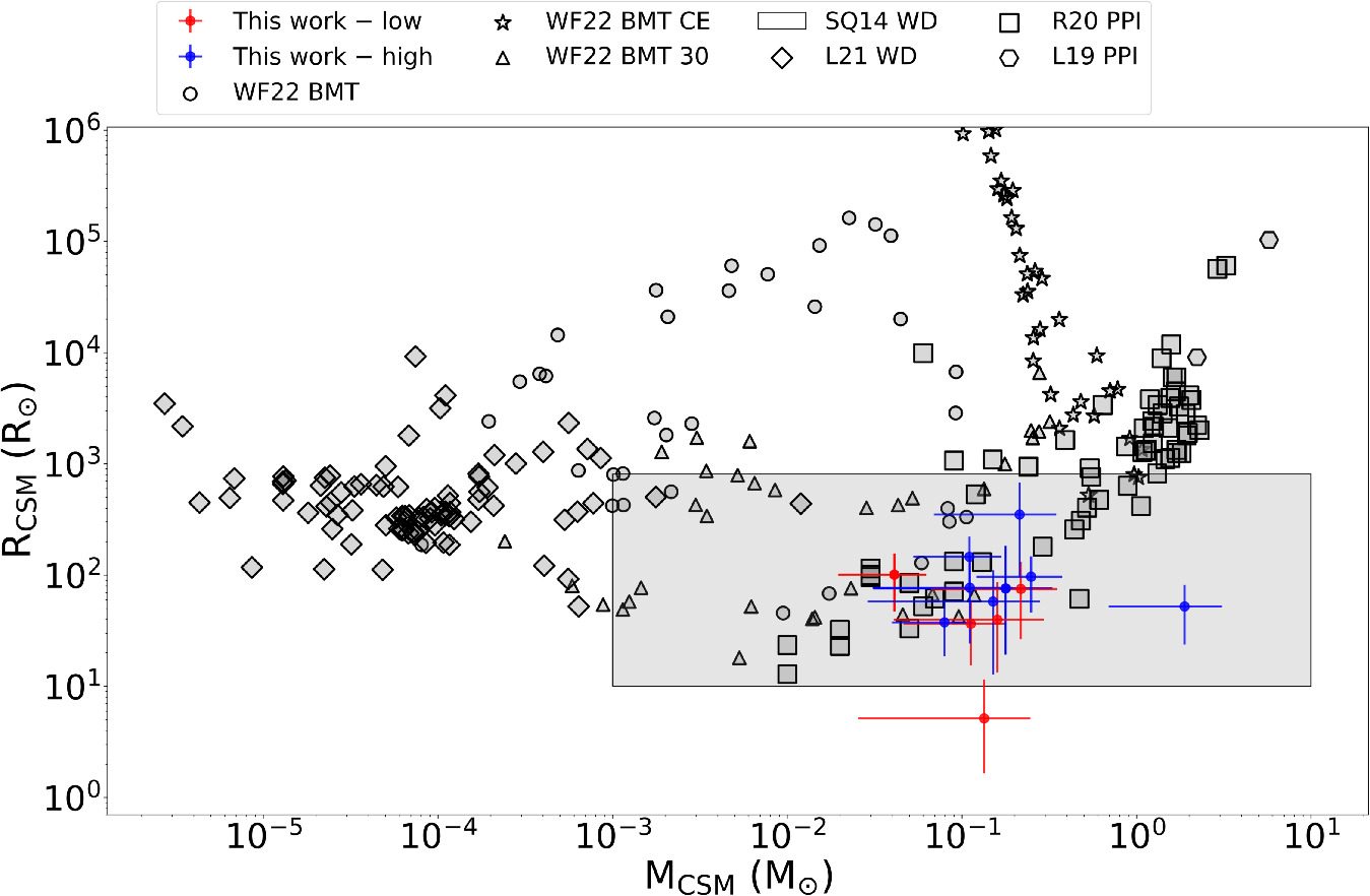
Figure 12. Comparison of the envelope parameters derived using the analytical shock-cooling model as described in Section 4.4.2 (red crosses) with unbound CSM predictions from various pre-SN mass-loss models: late-time stable binary mass transfer (BMT; Wu & Fuller 2022b), late-time unstable binary mass transfer via common envelope (BMT CE; Wu & Fuller 2022b), late-time binary mass transfer with shock breakout at an optical depth of ∼30 (BMT 30; Wu & Fuller 2022b), wave-driven mass loss (WD; Shiode & Quataert 2014; Leung et al. 2021a), and pulsation-pair instability-driven mass loss (PPI; Leung et al. 2019; Renzo et al. 2020). The SNe with low progenitor masses (≲12 M⊙) and higher progenitor masses are shown in red and blue, respectively.
Download figure:
Standard image High-resolution imageThese models have small SN ejecta masses of ≲1.5 M☉, assuming a neutron star mass of MNS = 1.4 M☉ consistent with the measured ejecta masses for SN 2021gno, SN 2021niq, SN 2021inl, SN 2022nwx, SN 2018lqo, and SN 2019dge in our sample. We compare the CSM properties for these with those predicted from the late-time mass transfer simulations (see Figure 12). We also show the CSM properties expected in the case of unstable MT, which leads to a common-envelope event (see Wu & Fuller 2022a for details). We find that the CSM properties across both scenarios are consistent with the CSM masses (∼0.01–1 M☉) and radii (∼1011–1013 cm) inferred for those SNe with low ejecta mass.
However, as mentioned earlier, the late-time mass transfer only occurs for the low progenitor mass SNe. To explain the CSM properties for sources with high ejecta mass, we turn to other pre-SN mass-loss models.
6.5. Pre-SN Mass Loss for Higher Progenitor Masses
6.5.1. Wave Heating Process in Hydrogen-poor Stars
Wave-driven mass loss (Quataert & Shiode 2012; Shiode & Quataert 2014; Fuller 2017; Fuller & Ro 2018; Leung et al. 2021a; Wu & Fuller 2021) occurs when convective motions in the massive star’s core excite internal gravity waves during its late-phase nuclear burning. These gravity waves propagate through the radiative core and transmit some percentage of its energy into the envelope via acoustic waves, which can be sufficient to eject a substantial amount of mass.
We compare the CSM properties with mass-loss models in Leung et al. (2021b) in Figure 12. The wave heating process in massive hydrogen-poor stars was investigated by Leung et al. (2021b), who surveyed a range of stellar models with main-sequence progenitor masses from 20 to 70 M☉ and metallicity from 0.002 to 0.02. Most of these models predict CSM masses less than ∼10−2 M☉. The low mass makes just wave-driven mass loss an unlikely explanation for all the observed CSM masses. However, a few models predict somewhat higher wave energy fluxes, have a larger ejected mass (∼10−2 M☉), or have a very large RCSM ∼ 1014 cm. These are models with large wave energies or long wave heating timescales, respectively. It requires the merger of nearby burning shells, in their models the carbon and helium shells. The merging of the two shells allows gravity waves to propagate across the star with a lower evanescence. However, numerical models show that such a phenomenon only occurs at individual masses of massive stars rather than a robust mass range. This may be consistent with the rarity of SNe observed in this work.
We find that the CSM properties predicted in Shiode & Quataert (2014) are consistent with our observations (see Figure 12). Shiode & Quataert (2014) predict that wave excitation and damping during Si burning can inflate nominally compact W-R progenitors to 10−3–1 M⊙ of the envelope of W-R stars to tens to hundreds of R⊙. These findings indicate that certain SN progenitors, often characterized by their compact nature, including those associated with Type Ibc SNe, exhibit a shock-cooling signature that differs considerably from conventional assumptions. The authors predict that the outcome of wave energy deposition during silicon fusion in W-R progenitors would probably manifest as a CCSN classified spectroscopically as Type Ibc (i.e., a compact star) but displaying early thermal emission reminiscent of extended stellar envelopes, which is observed as an early bump in our sample. However, we note that their estimates do not involve hydrodynamical simulations.
6.5.2. Pulsation-pair Instability
For very massive stars (MZAMS = 80–140 M☉), the electron–positron pair instability (PPI) drives explosive O burning and mass ejection, which accounts for an outburst of ∼0.1 to tens of M☉ (Leung et al. 2019; Woosley 2019; Renzo et al. 2020). Pulsation-induced mass loss relies on the electron–positron pair-creation catastrophe that happens in very massive stars (Heger & Woosley 2002). The star can experience several mass-loss events, depending on the available carbon and oxygen in the core (Woosley 2017; Leung & Fuller 2020).
In Figure 12, we plot the predicted CSM properties for the PPI-driven mass loss from Leung et al. (2019) and Renzo et al. (2020). The models center around MCSM ∼ 0.01–10 M☉ and RCSM ∼ 1011–1015 cm. These are consistent with the observed CSM properties for our sample (see Figure 12). The objects in this work are consistent with the lower-mass PPI SNe reported in the literature near a He core mass of ∼40 M⊙ (or ZAMS mass of ∼80 M⊙). We notice that the PPI SN model will be in tension for the objects with a low ejecta mass reported in this work. Given the high progenitor mass for PPI SNe (80–140 M⊙) and the production 56Ni, which indicates a robust explosion, if a spherical explosion is considered, the ejecta mass would be much larger. Most PPI SN models predict that the star will collapse into a black hole. The low ejecta mass could be explained if most of the star’s mass falls into the black hole and only a small fraction of the mass is ejected during the SN explosion. It is also possible that the aspherical explosion plays a role here. Through a jetlike energy deposition, only matter along the jet opening angle acquires the energy deposition; thus, the necessary energy deposition and the corresponding ejecta mass can be substantially lower even when the progenitor mass is high. Then, a relatively lower amount of energy is needed for the same ejecta velocity. The aspherical shape may lead to strong polarity in the optical signals, which can be checked for such sources in the future. Further samples along the trend may provide further evidence for PPI SNe being a robust production mechanism for low-mass CSM. However, given its high progenitor mass, which is less common in the stellar population according to the Salpeter relation, further comparison with the canonical SN rate will be important to check the compatibility of this picture with the stellar statistics. If we assume a Salpeter IMF, roughly ∼2.3% of CCSNe should undergo PPI, which is roughly consistent with the rate predicted for the double-peaked Type Ibc SNe in Section 2.
6.5.3. W-R+Red Supergiant Wind Mass Loss
One possibility is that the progenitors of our observed sources underwent a typical phase of red supergiant (RSG) with line-driven wind mass loss. Assuming a wind velocity (vw
) of ≈10 km s−1, the expected mass-loss rates range from  M☉ yr−1 to
  M☉ yr−1 (e.g., de Jager et al. 1988; Marshall et al. 2004; van Loon et al. 2005).
Subsequently, there is a relatively brief phase of W-R, characterized by higher wind velocities of a few thousand km s−1 and mass-loss rates around ∼10−5 M☉ yr−1 (e.g., Crowther 2007). It is a possibility that the stellar progenitor explodes as a Type Ibc SN within the bubble formed by its own W-R winds interacting with the prior RSG wind phase. However, the documented cases of W-R–RSG wind–wind interaction are associated with “bubbles” at typical distances of ∼1019 cm (Marston 1997), significantly farther than the few <1015 cm distances inferred for our sources. For our sample, the proximity of the CSM shell implies an extremely short W-R phase with a duration of ∼103 (v ∼ 1000 km s−1) yr, conflicting with the ∼105 yr duration of the W-R phase expected in the case of isolated massive stars. For such a short lifespan, assuming a mass-loss rate of ∼10−5 M⊙ yr−1, the mass loss will be around 0.01 M⊙, which is an order or so less than what we observe. Thus, wind loss from W-R+RSG is not consistent with our observations.
6.6. White Dwarf Progenitor
In the earlier sections, we discussed the presence of the early shock-cooling signatures as originating from the extended envelope or CSM of a massive progenitor star. However, we note that an early excess in the lightcurve is also possible in the context of a white dwarf. Such scenarios include white dwarf systems that involve companion interaction through Roche-lobe overflow (Kasen 2010; Magee et al. 2020), clumpy nickel distribution in the ejecta (Magee & Maguire 2020), and CSM interaction (Piro & Morozova 2016). The ejecta mass and oxygen mass measured for SN 2021gno, SN 2021niq, SN 2021inl, SN 2019dge, and SN 2018lqo are within the mass limit for a white dwarf. Based on the strong [Ca ii] emission lines in the nebular spectra, SN 2021gno, SN 2021inl, SN 2018lqo, and SN 2022oqm could belong to the thermonuclear group of Ca-rich gap transients, which result from explosive burning of He shells on the surface of low-mass white dwarfs (De et al. 2020). Jacobson-Galán et al. (2022b) favored a low-mass hybrid He/C/O + C/O white dwarf binary progenitor system for SN 2021gno and SN 2021inl based on the environment of their explosion sites. The disruption of a C/O white dwarf by a heavier white dwarf companion is favored for SN 2022oqm in Irani et al. (2024). Detailed spectral and lightcurve analysis in the context of the various white dwarf progenitor channels is left for future work.
7. Summary and Future Goals
- 1.We present a sample of 17 double-peaked Type Ibc(BL) SNe from ZTF. This was selected from a sample of 475 SNe classified as Ibc(BL) as part of the ZTF and CLU surveys. Out of these 475 SNe, there were 144 SNe with well-sampled early lightcurves. The rate of this sample is ∼3%–9% of Type Ibc(BL) SNe.The first peak is likely produced after the shock wave runs through an extended envelope and the layer cools (the “shock-cooling” phase). Type Ibc SNe are thought to arise from compact stars, so the envelope is more likely to be stellar material that was ejected in some mass-loss episode.
- 2.The peak magnitude of the first peak ranges from −14.2 to −20.1. We find that the peak magnitudes of the first peak and second peak are correlated as M2 = 0.8 × M1–4.7, where M1 and M2 are the peak magnitudes of the first and second peak, respectively. The correlation could imply that the SNe that show double-peaked lightcurves have He-star progenitors that shed their envelope in binary interactions. The photospheric velocities of the SNe in our sample are consistent with those of canonical Type Ibc SNe.
- 3.Based on nebular spectra and lightcurve properties, we divide our sample into two groups: six SNe (SN 2021gno, SN 2018lqo, SN 2021inl, SN 2022nwx, SN 2019dge, and SN 2021niq) with progenitor mass less than ∼12 M⊙ and ejecta mass less than 1.5 M⊙ and the rest with higher progenitor mass.
- 4.The observed CSM properties for SNe with low progenitor and ejecta mass might be explained as due to the binary evolution of low-mass He stars due to late-time mass transfer. The observed CSM properties of SNe with higher ejecta mass are consistent with certain models of wave-driven mass loss due to Si burning or pulsation-pair instability-driven mass loss.
The sample presented in this paper will enable detailed modeling of the progenitor and SN, offering insights into their mass-loss histories and envelope structures, and thus inform stellar evolution models. The investigation of double-peaked Type Ibc SNe and the mechanisms behind pre-SN mass loss have implications across multiple areas of astronomy. These findings have the potential to alter predictions related to ionizing radiation and wind feedback from stellar populations, thereby influencing conclusions about star formation rates and initial mass functions in galaxies beyond our own. Moreover, these discoveries impact our understanding of the origins of diverse compact stellar remnants and shape the way we utilize SNe as tools for studying stellar evolution throughout cosmic history
While analytical modeling of shock cooling provides a good estimate of the CSM properties, it might not be able to take into account detailed nuances such as variable opacities, densities, etc. The exact structure of the CSM and its impact on the explosion lightcurve require detailed hydrodynamics and radiative transfer calculations, which we leave for future work.
It is also important to understand the implication of the missing early bump in the majority of Type Ibc SNe in understanding the multiplicity of stars, binary evolution, and the extent of stripping in compact binaries including common-envelope evolution. Further theoretical work to study this is left for future work.
This sample shows that shock-cooling emission may be very common in H-poor SNe. We might be missing many of them because of poor early-time cadence. Early observations with future wide-field UV surveys such as ULTRASAT (Sagiv et al. 2014; Shvartzvald et al. 2024) and UVEX (Kulkarni et al. 2021) will be critical for the discovery and study of these SNe. Also, X-ray and radio follow-up observations (Matsuoka & Maeda 2020; Kashiyama et al. 2022) of H-poor SNe with well-sampled early optical lightcurves will help better constrain the mass-loss mechanisms.
Acknowledgments
We thank Anthony L. Piro for insightful discussions and comments. We would also like to thank Daniel Brethauer for providing the data used in Brethauer et al. (2022). Based on observations obtained with the Samuel Oschin Telescope 48 inch and the 60 inch telescope at the Palomar Observatory as part of the Zwicky Transient Facility project. ZTF is supported by the National Science Foundation under grant No. AST-2034437 and a collaboration including Caltech, IPAC, the Weizmann Institute of Science, the Oskar Klein Center at Stockholm University, the University of Maryland, Deutsches Elektronen-Synchrotron and Humboldt University, the TANGO Consortium of Taiwan, the University of Wisconsin at Milwaukee, Trinity College Dublin, Lawrence Livermore National Laboratories, IN2P3, France, the University of Warwick, the University of Bochum, and Northwestern University. Operations are conducted by COO, IPAC, and UW.
SED Machine is based upon work supported by the National Science Foundation under grant No. 1106171.
The ZTF forced-photometry service was funded under the Heising-Simons Foundation grant No. 12540303 (PI: Graham).
The GROWTH Marshal was supported by the GROWTH project funded by the National Science Foundation under grant No. 1545949.
The data presented here were obtained in part with ALFOSC, which is provided by the Instituto de Astrofisica de Andalucia (IAA) under a joint agreement with the University of Copenhagen and NOT.
The Liverpool Telescope is operated on the island of La Palma by Liverpool John Moores University in the Spanish Observatorio del Roque de los Muchachos of the Instituto de Astrofisica de Canarias with financial support from the UK Science and Technology Facilities Council. Based on observations made with the Italian Telescopio Nazionale Galileo (TNG) operated on the island of La Palma by the Fundación Galileo Galilei of the INAF (Istituto Nazionale di Astrofisica) at the Spanish Observatorio del Roque de los Muchachos of the Instituto de Astrofisica de Canarias.
The W. M. Keck Observatory is operated as a scientific partnership among the California Institute of Technology, the University of California, and the National Aeronautics and Space Administration. The Observatory was made possible by the generous financial support of the W. M. Keck Foundation. The authors wish to recognize and acknowledge the very significant cultural role and reverence that the summit of Maunakea has always had within the indigenous Hawaiian community. We are most fortunate to have the opportunity to conduct observations from this mountain. The ztfquery code was funded by the European Research Council (ERC) under the European Union’s Horizon 2020 research and innovation program (grant agreement No. 759194−USNAC; PI: Rigault).
S.-C. L. acknowledges the support by the National Science Foundation under Grant AST-2316807.
Data Availability
All the photometric and spectroscopic data used in this work will be available here after publication.
The optical photometry and spectroscopy will also be made public through WISeREP, the Weizmann Interactive Supernova Data Repository (Yaron & Gal-Yam 2012).
Appendix A: Photometry Data
A summary of the photometry data used for SN 2018lqo (truncated) is provided in Table 10. The photometry data for all sources are provided as machine-readable tables in Zenodo via doi:10.5281/zenodo.11505429.
Table 10. Summary of the Photometry Data Used for SN 2018lqo (Truncated)
| Date | Filter | Instrument | Mag. | Limiting Mag. |
|---|---|---|---|---|
| (JD) | (AB mag) | (AB mag) | ||
| 2458340.68 | r | P48+ZTF | 20.11 ± 0.17 | 20.31 |
| 2458343.66 | r | P48+ZTF | 20.68 ± 0.23 | 20.64 |
| 2458343.68 | g | P48+ZTF | 20.98 ± 0.37 | 20.71 |
| 2458346.66 | g | P48+ZTF | 20.49 ± 0.30 | 20.49 |
| 2458346.68 | r | P48+ZTF | 20.16 ± 0.16 | 20.53 |
| 2458346.68 | r | P48+ZTF | 20.16 ± 0.16 | 20.53 |
| 2458347.76 | r | P60+SEDM | 20.02 ± 0.05 | 21.69 |
| 2458347.76 | r | P60+SEDM | 20.06 ± 0.04 | 99.00 |
| 2458347.76 | g | P60+SEDM | 20.40 ± 0.06 | 21.81 |
| 2458347.76 | g | P60+SEDM | 20.47 ± 0.07 | 99.00 |
| 2458347.76 | i | P60+SEDM | 19.92 ± 0.10 | 21.48 |
| 2458347.76 | i | P60+SEDM | 19.92 ± 0.53 | 99.00 |
| 2458348.68 | i | P48+ZTF | 19.82 ± 0.23 | 19.94 |
| 2458350.65 | r | P48+ZTF | 19.68 ± 0.16 | 20.45 |
Download table as: ASCIITypeset image
Appendix B: Lightcurves
The lightcurves of all sources can be found in Zenodo via doi:10.5281/zenodo.11505429.
Appendix C: Spectra
The spectra of all sources are provided as machine-readable tables in Zenodo via doi:10.5281/zenodo.11505429.
Appendix D: Blackbody Fits
A summary of the blackbody properties for SN 2018lqo (truncated) is provided in Table 11. All the best-fit parameters including bolometric luminosity, radius, and temperature for each object are provided as machine-readable tables in Zenodo via doi:10.5281/zenodo.11505429.
Table 11. Summary of the Blackbody Properties for SN 2018lqo (Truncated)
| Phase | Log Luminosity | Temperature | Radius |
|---|---|---|---|
| (days since first detection) | (erg s−1) | (K) | (R⊙) |
| 3.17 |

|

|

|
| 4.33 |

|

|

|
| 6.17 |

|

|

|
| 7.26 |

|

|

|
| 8.24 |

|

|

|
| 10.21 |

|

|

|
| 11.22 |

|

|

|
| 12.21 |

|

|

|
| 20.22 |

|

|

|
| 21.17 |

|

|

|
| 22.22 |

|

|

|
| 25.18 |

|

|

|
Download table as: ASCIITypeset image
Appendix E: First-peak fits
Figure 13 shows a collage of the best-fit lightcurves for the shock-cooling model (Piro et al. 2021) fits to the multiband photometry data.
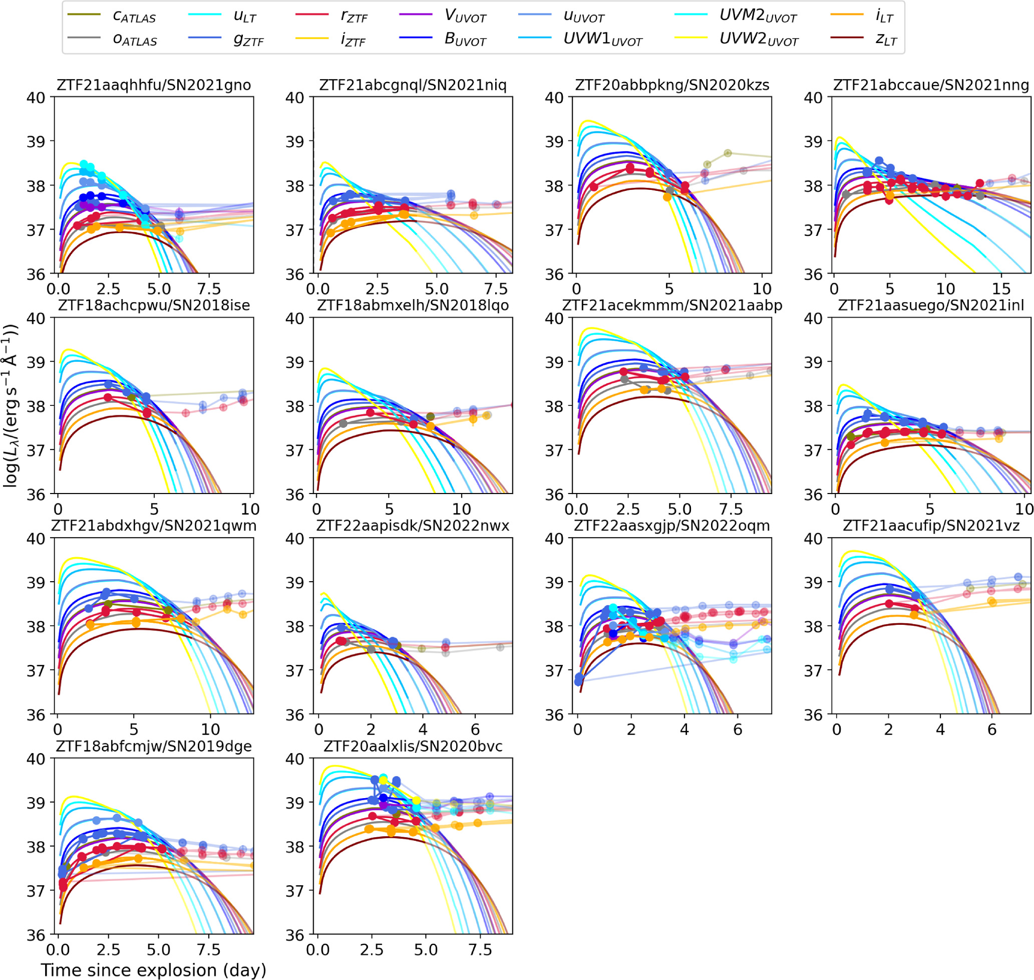
Figure 13. Shock-cooling model (Piro et al. 2021) fits to multiband data.
Download figure:
Standard image High-resolution imageAppendix F: Second-peak Fits
Figure 14 shows a collage of the best-fit lightcurves for the radioactive peak model (Arnett & Meakin 2011) fits to the bolometric luminosity data.
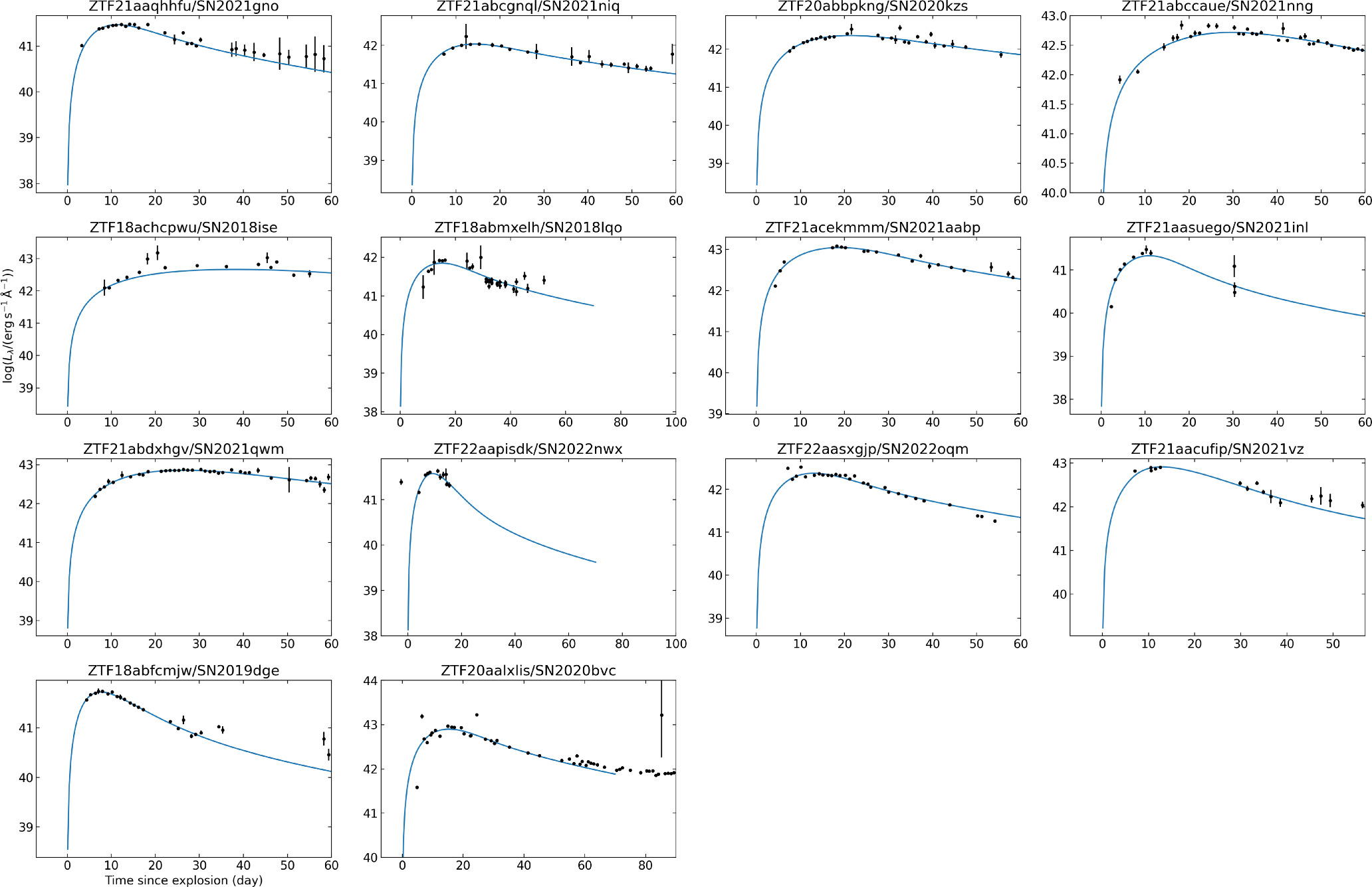
Figure 14. Radioactive (Arnett et al. 1989) fits to bolometric luminosity data.
Download figure:
Standard image High-resolution imageAppendix G: Spectral Log
The spectral log and velocity measurements are listed in Table 12.
Table 12. Spectral Log and Ejecta Velocity Measurements
| Source | Date | Phase | Inst. | He i λ5876 | O i λ7774 |
|---|---|---|---|---|---|
| (days) | (km s−1) | (km s−1) | |||
| ZTF21aaqhhfu/SN 2021gno | 2021-03-20 | −15.0 | SPRAT | ⋯ | 7910 ± 1170 |
| ZTF21aaqhhfu/SN 2021gno | 2021-03-21 | −14.0 | SEDM | ⋯ | ⋯ |
| ZTF21aaqhhfu/SN 2021gno | 2021-03-24 | −11.0 | SEDM | 12,850 ± 4520 | ⋯ |
| ZTF21aaqhhfu/SN 2021gno | 2021-04-02 | −2.0 | SPRAT | 8000 ± 260 | 6860 ± 810 |
| ZTF21aaqhhfu/SN 2021gno | 2021-04-02 | −2.0 | SEDM | 7880 ± 740 | 5830 ± 2610 |
| ZTF21aaqhhfu/SN 2021gno | 2021-04-12 | 8.0 | SEDM | 8210 ± 2540 | 7630 ± 2920 |
| ZTF21aaqhhfu/SN 2021gno | 2022-02-04 | 306.0 | LRIS | ⋯ | ⋯ |
| ZTF21abcgnql/SN 2021niq | 2021-05-31 | −6.0 | DBSP | 13,680 ± 2630 | ⋯ |
| ZTF21abcgnql/SN 2021niq | 2022-04-13 | 310.0 | LRIS | ⋯ | ⋯ |
| ZTF20abbpkng/SN 2020kzs | 2020-06-01 | −9.0 | SEDM | ⋯ | ⋯ |
Only a portion of this table is shown here to demonstrate its form and content. A machine-readable version of the full table is available.
Download table as: Machine-readable (MRT)Typeset image
Appendix H: Density Profile of He Stars Used in the Late-time Mass Transfer Models
The density profiles of the single He stars of different masses before late-time mass transfer used in Section 6.2 are shown in Figure 15. The density profiles of the bound material of the stars after mass transfer can be found in Zenodo via doi:10.5281/zenodo.11505429.
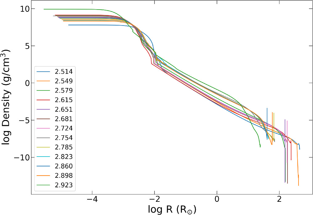
Figure 15. Density profile of the single He stars of different masses before late-time mass transfer used in Section 6.2.
Download figure:
Standard image High-resolution imageFootnotes
- 24
ZTF18acsodbf and ZTF19abzzuhj.
- 25
- 26
- 27