Abstract
We present Atacama Large Millimeter/submillimeter Array (ALMA) Cycle 2 observations of CO(2–1) emission from the circumnuclear disks in two early-type galaxies, NGC 1380 and NGC 6861. The disk in each galaxy is highly inclined (i ∼ 75°), and the projected velocities of the molecular gas near the galaxy centers are ∼300 km s−1 in NGC 1380 and ∼500 km s−1 in NGC 6861. We fit thin disk dynamical models to the ALMA data cubes to constrain the masses of the central black holes (BHs). We created host galaxy models using Hubble Space Telescope images for the extended stellar mass distributions and incorporated a range of plausible central dust extinction values. For NGC 1380, our best-fit model yields MBH = 1.47 × 10⁸ M⊙ with a ∼40% uncertainty. For NGC 6861, the lack of dynamical tracers within the BH’s sphere of influence due to a central hole in the gas distribution precludes a precise measurement of MBH. However, our model fits require a value for MBH in the range of (1–3) × 109 M⊙ in NGC 6861 to reproduce the observations. The BH masses are generally consistent with predictions from local BH–host galaxy scaling relations. Systematic uncertainties associated with dust extinction of the host galaxy light and choice of host galaxy mass model dominate the error budget of both measurements. Despite these limitations, the measurements demonstrate ALMA’s ability to provide constraints on BH masses in cases where the BH’s projected radius of influence is marginally resolved or the gas distribution has a central hole.
Original content from this work may be used under the terms of the Creative Commons Attribution 4.0 licence. Any further distribution of this work must maintain attribution to the author(s) and the title of the work, journal citation and DOI.
1. Introduction
Supermassive black holes (BHs) are believed to reside in the centers of all massive galaxies that are not pure disks. They encode information about the formation and evolution of their host galaxies through a number of scaling relations such as the MBH–σ⋆, MBH–Lbul, and MBH–Mbul relations (Kormendy & Richstone 1995; Gebhardt et al. 2000; Ferrarese & Merritt 2000; Kormendy & Ho 2013), which relate BH mass to spheroid stellar velocity dispersion, luminosity, and mass. These scaling relations are often used to estimate BH masses in galaxies over broad ranges in both galaxy type and distance (Kormendy & Ho 2013; McConnell & Ma 2013; Saglia et al. 2016; van den Bosch et al. 2016).
Increasing the sample of measured BH masses that define these scaling relations is necessary to improve our understanding of BH–host galaxy coevolution. Questions regarding when these scaling relations came to be, the ranges of BH masses and galaxy types they apply to, and the physical mechanisms that allowed them to form remain unanswered. To complicate matters, MBH predictions from the MBH–σ⋆ and MBH–Lbul relations can strongly disagree, such as in the case of the most luminous early-type galaxies (ETGs), where the discrepancies reach an order of magnitude at MBH ∼ 1010 M⊙ (Bernardi et al. 2007; Lauer et al. 2007). A larger sample of reliable BH mass measurements is needed to address these questions and issues.
About 100 supermassive BH mass measurements have been obtained through modeling the motions of either stars or gas (Kormendy & Ho 2013). Accurately determining these masses requires modeling the motions of kinematic tracers that extend within the BH’s radius of influence,  , where the BH as opposed to the host galaxy is the main contributor to their combined gravitational potential. Among current measurements, the most robust are of the Milky Way’s own supermassive BH (Boehle et al. 2016; Gravity Collaboration et al. 2019), which use observations of individual stellar orbits, and of BHs in galaxies with rotating H2O megamaser disks whose emission originates deep within rg
(Miyoshi et al. 1995; Kuo et al. 2011, 2018). For other galaxies, BH masses have been measured primarily through stellar-dynamical and ionized gas-dynamical modeling. Both methods are prone to a variety of challenges in modeling and interpreting the data. Stellar-dynamical modeling of massive ETGs is sensitive to the treatment of galaxy triaxiality, dark matter halo structure, and stellar orbital anisotropy (van den Bosch et al. 2008; Gebhardt & Thomas 2009; Shen & Gebhardt 2010), while ionized gas-dynamical modeling can be affected by noncircular motions and substantial gas turbulence (Barth et al. 2001; Shapiro et al. 2006).
, where the BH as opposed to the host galaxy is the main contributor to their combined gravitational potential. Among current measurements, the most robust are of the Milky Way’s own supermassive BH (Boehle et al. 2016; Gravity Collaboration et al. 2019), which use observations of individual stellar orbits, and of BHs in galaxies with rotating H2O megamaser disks whose emission originates deep within rg
(Miyoshi et al. 1995; Kuo et al. 2011, 2018). For other galaxies, BH masses have been measured primarily through stellar-dynamical and ionized gas-dynamical modeling. Both methods are prone to a variety of challenges in modeling and interpreting the data. Stellar-dynamical modeling of massive ETGs is sensitive to the treatment of galaxy triaxiality, dark matter halo structure, and stellar orbital anisotropy (van den Bosch et al. 2008; Gebhardt & Thomas 2009; Shen & Gebhardt 2010), while ionized gas-dynamical modeling can be affected by noncircular motions and substantial gas turbulence (Barth et al. 2001; Shapiro et al. 2006).
Molecular gas has emerged as a dynamical tracer capable of circumventing the aforementioned issues with stellar-dynamical and ionized gas-dynamical modeling. Tracers such as H2, HCN, HCO+, and CO emission lines have been used to constrain BH masses in late-type galaxies (Neumayer et al. 2007; Scharwächter et al. 2013; Onishi et al. 2015; den Brok et al. 2015). In addition, a number of CO surveys have shown that a fraction of ETGs have dynamically cold and regularly rotating molecular gas disks at their centers (Combes et al. 2007; Young et al. 2011; Alatalo et al. 2013; Bolatto et al. 2017). These molecular gas disks are ideal targets for precision BH mass measurements. As with ionized gas, modeling the dynamics of molecular gas on scales comparable to the BH’s sphere of influence is insensitive to factors such as the distribution of dark matter and triaxial structure, which affect stellar-dynamical models. Molecular gas also has the added benefit that it is much less turbulent than ionized gas (Davis et al. 2013a; Utomo et al. 2015; Boizelle et al. 2017).
Davis et al. (2013b) demonstrated the potential of molecular gas as an effective kinematic tracer by measuring the mass of the BH in NGC 4526 with the Combined Array for Millimeter-wave Astronomy. Since then, the Atacama Large Millimeter/submillimeter Array (ALMA) has emerged as the premier radio interferometer for these types of measurements. There are now several ALMA-based BH mass measurements derived from observations of molecular gas emission on scales comparable to and even within the BHs’ spheres of influence for nearby galaxies (Barth et al. 2016a; Davis et al. 2017; Onishi et al. 2017; Boizelle et al. 2019; Smith et al. 2019; North et al. 2019; Boizelle et al. 2021; Cohn et al. 2021; Nguyen et al. 2021).
In this paper, we analyze ALMA observations of NGC 1380 and NGC 6861, two galaxies that have been shown to host a central circumnuclear gas disk. Boizelle et al. (2017) mapped the distribution of CO(2–1) emission within these disks and found that they exhibited dynamically cold rotation.
NGC 1380 is classified as an SA0 galaxy in both the Third Reference Catalogue of Bright Galaxies (RC3; de Vaucouleurs et al. 1991) and in the Hyperleda database (Paturel et al. 2003). It is located at a luminosity distance of 17.1 Mpc in the Fornax cluster based on surface brightness fluctuations from Tonry et al. (2001) after applying the Cepheid zero-point correction from Mei et al. (2007). With this assumed luminosity distance, and using an observed redshift of z = 0.00618 obtained from initial dynamical modeling results, the corresponding angular scale is 81.9  . We adopt the Hyperleda average stellar velocity dispersion of σ⋆ = 215 km s−1 (Makarov et al. 2014), a total apparent K-band magnitude of mK
= 6.87 mag from the Two Micron All Sky Survey (2MASS; Jarrett et al. 2003) and a bulge-to-total ratio of B/T = 0.34 from the Carnegie-Irvine Galaxy Survey (Gao et al. 2019).
. We adopt the Hyperleda average stellar velocity dispersion of σ⋆ = 215 km s−1 (Makarov et al. 2014), a total apparent K-band magnitude of mK
= 6.87 mag from the Two Micron All Sky Survey (2MASS; Jarrett et al. 2003) and a bulge-to-total ratio of B/T = 0.34 from the Carnegie-Irvine Galaxy Survey (Gao et al. 2019).
NGC 6861 is located at a luminosity distance of 27.3 Mpc in the Telescopium galaxy group, which corresponds to an angular scale of 129.9  when using a redshift of z = 0.00944 from our initial dynamical models. This galaxy is classified as an E/S0 in Hyperleda and as an S0A-(s) in RC3. Kormendy & Ho (2013) noted that the main body of NGC 6861 does not deviate significantly from an n ≃ 2 Sérsic-function profile, although the galaxy has extra central light; we adopt that paper’s classification as an extra-light elliptical. In addition, we also adopt the stellar velocity dispersion of σ⋆ = 389 km s−1 measured within the effective radius by Rusli et al. (2013), and the 2MASS total apparent K-band magnitude of mK
= 7.75 mag (Vaddi et al. 2016).
when using a redshift of z = 0.00944 from our initial dynamical models. This galaxy is classified as an E/S0 in Hyperleda and as an S0A-(s) in RC3. Kormendy & Ho (2013) noted that the main body of NGC 6861 does not deviate significantly from an n ≃ 2 Sérsic-function profile, although the galaxy has extra central light; we adopt that paper’s classification as an extra-light elliptical. In addition, we also adopt the stellar velocity dispersion of σ⋆ = 389 km s−1 measured within the effective radius by Rusli et al. (2013), and the 2MASS total apparent K-band magnitude of mK
= 7.75 mag (Vaddi et al. 2016).
For each galaxy, we obtained a BH mass by constructing gas-dynamical models and fitting directly to the ALMA data cubes. This work provides the first dynamical mass measurement of the supermassive BH in NGC 1380, and a second, independent dynamical mass measurement of the supermassive BH in NGC 6861, which was previously measured through stellar-dynamical modeling to be (2.0 ± 0.2) × 109 M⊙ by Rusli et al. (2013).
Our paper is organized as follows. In Section 2, we describe both the Hubble Space Telescope (HST) and ALMA observations and the data reduction process. In Section 3, we decompose the stellar surface brightness distribution of each galaxy with Multi-Gaussian expansions and construct extinction-corrected host galaxy models. A description of our dynamical modeling formalism, including the thin disk model, is presented in Section 4. We present and compare the results of our dynamical models in Section 5. In Section 6, we compare our measurements of MBH to the local BH–host galaxy scaling relations and discuss limiting factors in the measurements. We conclude and summarize our findings in Section 7.
2. Observations
2.1. HST Data
For NGC 1380, we retrieved and used archival HST F160W (H-band) images from HST program 11712. The observation was subdivided into four separate exposures of 299 s each that were taken with the Wide Field Camera 3 (WFC3). We processed the images with the calwf3 pipeline and subsequently combined them in AstroDrizzle to produce a cleaned and distortion-corrected image with a pixel scale of 008 pixel−1. We followed a similar procedure for NGC 6861. We used archival HST data for NGC 6861 from Program 15226, which was designed to obtain host galaxy imaging to complement our ALMA program. The observation consisted of four separate exposures of 249 s each taken with the F160W filter on WFC3. We processed and combined the images with calwf3 and AstroDrizzle to produce a composite image with a 0
08 pixel−1 scale. To identify regions of substantial dust attenuation, we also obtained archival F110W (J-band) images for each galaxy. Archival F110W observations of NGC 1380 were obtained from HST program 11712 and consisted of four separate exposures of 299 s each, while F110W observations of NGC 6861 were obtained from HST program 15226 and consisted of two separate exposures of 249 s each. These were processed using the calwf3 pipeline and AstroDrizzle as above.
2.2. ALMA Data
2.2.1. Observations and Data Reduction
We obtained ALMA imaging of NGC 1380 and NGC 6861 as part of Program 2013.1.00229.S. The data were studied by Boizelle et al. (2017) as part of a larger sample of galaxies to map CO(2–1) emission in nearby ETGs, and we review their data reduction process and findings below.
NGC 1380 was observed in ALMA Band 6 for 23 minutes on both 2015 June 11 and 2015 September 18 with maximum baselines of 783 m and 2125 m, respectively. For the redshifted 12CO(2–1) line, the observation covered a 1.875 GHz bandwidth from 228.199 to 230.074 GHz, centered at an estimated redshifted line frequency of 229.136 GHz. The frequency channel widths were 488.281 kHz, corresponding to a velocity channel resolution of 0.64 km s−1 at the redshifted frequency. For continuum emission, two separate 2 GHz spectral windows were centered at 227.210 and 244.902 GHz with 15.625 MHz channel widths, equating to velocity resolutions of 20.6 and 19.1 km s−1, respectively. The data were initially processed through the ALMA pipeline with version 4.3.1 of the Common Astronomy Software Applications package (CASA; McMullin et al. 2007) and then imaged into data cubes using Briggs weighting with a robust parameter of 0.5 following continuum phase self-calibration and continuum subtraction in the uv plane. We reimaged the cube to have 10 km s−1 velocity channel widths (with respect to the rest frequency of the 12CO(2–1) line) to isolate narrower line features in spatial regions close to the disk center and chose a pixel size of 003 to sufficiently sample the synthesized beam’s minor axis. The beam’s FWHM is 0
24 and 0
18 along the major and minor axis, respectively, and the beam has a position angle of 86
9 measured east of north.
NGC 6861 was observed on 2014 September 1 in ALMA Band 6 for 24 minutes with a maximum baseline of 1091 m. The line observation was centered at an estimated redshifted 12CO(2–1) line frequency of 228.390 GHz, while the continuum windows were centered at 226.466 and 244.098 GHz, with the same bandwidth and channel spacing properties as the NGC 1380 observation. The data were processed using CASA version 4.2.2 and imaged into a data cube with 20 km s−1 velocity channel widths following the continuum phase self-calibration and continuum subtraction processes described for the NGC 1380 data. The NGC 6861 data cube has the following properties: a synthesized beam size of 032 × 0
23 with a position angle of 58
2 and a pixel size of 0
065.
2.2.2. Circumnuclear Disk Properties
Boizelle et al. (2017) determined several properties of the circumnuclear disks in NGC 1380 and NGC 6861, which we summarize here. The gas in each disk is cospatial with the dust, as seen in the HST optical images and ALMA integrated intensity maps in Figure 1. Both disks are very inclined (i ≈ 75°) and exhibit orderly rotation around their respective centers, with projected line-of-sight (LOS) velocities of ∼300 km s−1 and ∼500 km s−1 for NGC 1380 and NGC 6861, respectively. LOS velocity and dispersion maps indicate nearly circular and dynamically cold rotation about the disk centers. Independent stellar kinematic observations with the Multi Unit Spectroscopic Explorer (MUSE) have also revealed the presence of a large-scale cold disk component in NGC 1380 (Sarzi et al. 2018). The radial extents of the CO emission were measured to be 52 (426 pc) and 6″ (784 pc) for NGC 1380 and NGC 6861, respectively. A major axis position–velocity diagram (PVD) extracted from the NGC 1380 data cube shows a slight rise in velocity within the innermost ∼0
1, although this does not extend past the velocities observed in the outer parts of the PVD. This central upturn in gas velocity indicates the presence of a massive and compact object at the disk center. For NGC 6861, the PVD and moment maps reveal a central ∼1″ radius hole in CO emission. The gas mass of each disk was determined by summing the CO flux and assuming an αCO factor of 3.1 M⊙ pc−2 (K km s−1)−1 (Sandstrom et al. 2013) as the extragalactic mass-to-luminosity ratio, a CO(2–1)/CO(1-0) ≈ 0.7 line ratio in brightness temperature units (Lavezzi et al. 1999), and a correction factor of 1.36 for helium. Given these assumptions, the gas masses were estimated to be (8.4 ± 1.6) ×107
M⊙ and (25.6 ± 8.9) × 107
M⊙ for NGC 1380 and NGC 6861, respectively. For NGC 1380, our assumption about CO excitation can be tested: Zabel et al. (2019) measured a CO(1–0) line flux for NGC 1380 that, in combination with the CO(2–1) line flux from Boizelle et al. (2017), implies a CO(2–1)/CO(1–0) ratio of
 in brightness temperature units. This is higher than our assumed value of 0.7, and implies a lower gas mass. Because a ratio >1 is unphysically high if both CO lines are tracing the same material, we consider a value ≈0.9 (still lying within the measurement uncertainties) to be more appropriate and in Section 5.2 explore the implications of the correspondingly lower gas mass for our dynamical models.
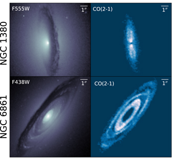
Figure 1. Images of NGC 1380 and NGC 6861 from HST and ALMA observations showing the cospatial distributions of the dust and gas. The left panels show F555W and F438W HST observations of the dust disks in NGC 1380 and NGC 6861, respectively. For each image, north is up and east is to the left. The ALMA intensity maps in the right panels were created by summing across channels after using the 3DBarolo program (Di Teodoro & Fraternali 2015) to generate a mask that identified pixels with CO emission.
Download figure:
Standard image High-resolution image3. Host Galaxy Surface Brightness Modeling
A key input to the dynamical modeling program is the stellar mass profile, M⋆(r), which is determined by measuring and deprojecting the host galaxy’s observed surface brightness profile. One approach to obtaining M⋆(r) is the Multi-Gaussian expansion (MGE) method, which fits the observed brightness in galaxy images with a series expansion of 2D Gaussian functions (Emsellem et al. 1994; Cappellari 2002). For galaxies such as NGC 1380 and NGC 6861, which possess optically thick dust disks, the impact of dust attenuation on the host galaxy light is mitigated by using observations in the near-infrared (NIR) regime, but the impact is not completely negligible. To assess the variation of H-band extinction across the dust disk, we performed a simple correction to the observed H-band major axis surface brightness profile for each galaxy as described in Section 3.1. This was done as an attempt to quantify the possible impact of dust on the host galaxy’s surface brightness. We then proceeded to fit dust-masked and dust-corrected MGE models to the drizzled H-band images of NGC 1380 and NGC 6861, as described in Sections 3.2 and 3.3.
3.1. Major Axis Dust Extinction Corrections
The central dust disk in each galaxy is clearly visible in Figures 1 and 2, due to its dimming and reddening of the observed stellar light. We attempted to estimate the amount of dust extinction with a color-based correction method, which was complicated by the fact that the dust disk is embedded within the galaxy and cannot be treated as a simple foreground screen. To estimate the amount of dust extinction, we extracted and corrected the observed H-band major axis surface brightness profile of each galaxy. Using the sectors_photometry routine from the MgeFit package in Python (Cappellari 2002), we plotted the surface brightness profile of each galaxy in Figure 3. In NGC 1380, a slight dip in the profile can be seen at around r = 4″, which marks the outer edge of the dust disk, while a more noticeable dip is seen between ∼1″ and 55 in NGC 6861.
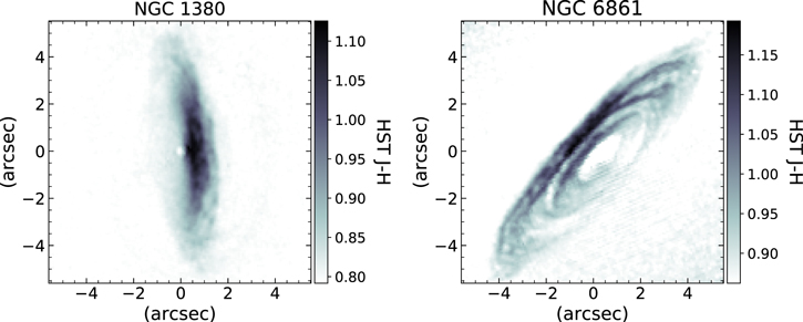
Figure 2. NGC 1380 (left) and NGC 6861 (right) J − H color maps constructed using WFC3 F110W and F160W observations. The maps highlight the color asymmetries of the near and far sides of the disks, with the near sides being ∼0.2–0.3 mag redder than the far sides. For NGC 6861, a 1″ radius hole in the center of the dust distribution can be seen.
Download figure:
Standard image High-resolution image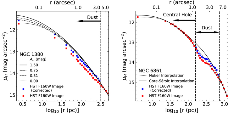
Figure 3. Comparison of the observed NGC 1380 (left) and NGC 6861 (right) HST major axis H-band surface brightness profiles to their respective dust-corrected models. The red points are the observed values from the H-band images, while the blue points are the dust-corrected values described in Section 3.1. The different lines in each panel correspond to extracted major axis surface brightness profiles for our 2D MGE models, which are described in Sections 3.2 and 3.3. For NGC 1380, we mark the outer edge of the dust disk with a vertical dashed line and indicate that the dust extends down to the nucleus with an arrow, while for NGC 6861, we indicate the inner and outer boundaries of the dusty region with the two dashed lines.
Download figure:
Standard image High-resolution imageTo determine the pixels that are most affected by dust, we created J − H color maps as seen in Figure 2. We note that all H- and J-band magnitudes in this work are in the Vega magnitude system. The color maps revealed that the dust extends from the nuclei, and the pixels most affected by dust are about 0.25 mag redder than the median J − H color of ∼0.80 mag outside the disk. Furthermore, each nucleus has a bluer color that is nearly identical to the median color outside the disk. A blue nucleus suggests the presence of star formation or a weak active galactic nucleus (AGN); we discuss these possibilities below.
We attempted to correct the major axis H-band surface brightness profiles by examining Δ(J − H), the observed color excess relative to the median J − H color outside the disk, along the major axis. Using Equation (1) from Boizelle et al. (2019), which predicts the ratio of observed to intrinsic integrated stellar light based on the embedded-screen model described by Viaene et al. (2017), we generated a model Δ(J − H) curve as a function of intrinsic V-band extinction, AV , to compare with the observations.
The embedded-screen model assumes that the obscuring dust lies in a thin, inclined disk that bisects the galaxy, and that the fraction of stellar light originating behind the disk, b, is obscured by simple screen extinction, while the fraction of stellar light in front of the disk, f, is unaffected. In addition, the model assumes that there is no scattering of stellar light back into the LOS, and that the J − H color outside of the disk is the intrinsic color of the host galaxy. One important aspect of this color excess model is that Δ(J − H) is not a strictly monotonically increasing function of intrinsic extinction. As seen in Figure 4, the color excess increases approximately linearly with increasing AV up to a turnover point, after which it will begin to decrease to zero as the light originating behind the disk becomes completely obscured. As a result, there are two possible AV values for a given Δ(J − H). To maintain a one-to-one correspondence between Δ(J − H) and AV , we considered only the low-extinction branch of the curve and therefore adopted the lesser of the two possible AV values. We inverted the relationship to derive AV as a function of observed Δ(J − H) by fitting a third-order polynomial up to the turnover point and determining its inverse. Using a standard Galactic (RV = 3.1) extinction curve (Rieke & Lebofsky 1985) where AH /AV = 0.175, and assuming that the fractions of stellar light originating in front of and behind the disk are equal (f = b = 0.5) along the major axis, we associated our observed major axis Δ(J − H) values with corresponding values of AH .
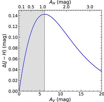
Figure 4. Modeled Δ(J − H) curve as a function of AV (bottom axis) and AH (top axis). The curve was generated using Equation (1) from Boizelle et al. (2019) and a standard Galactic (RV = 3.1) extinction curve (Rieke & Lebofsky 1985), under the assumptions that along the major axis, the fractions of light in front of and behind the disk are equal (f = b = 0.50), and that only the starlight originating from behind the disk is subject to dust extinction. The gray region left of the dotted line indicates the part of the curve we used to define a one-to-one correspondence between Δ(J − H) and AV and AH for the low-extinction branch of the curve.
Download figure:
Standard image High-resolution imageWe generated point-by-point corrections to our major axis surface brightness profiles using the fact that our modeled AH values only applied to the fraction of light originating behind the disk. The corrected values are shown in blue in Figure 3 for points within the dust disk for each galaxy. For NGC 1380, the corrected surface brightness profile still exhibits a slight dip near the edge of the dust disk. For NGC 6861, where we can anchor the surface brightness profile inside and outside the dust disk, it is clear there is still some remaining extinction, as the decrease in observed surface brightness is still visible in the corrected profile.
Since the method described above appears to undercorrect for extinction, we also tried applying the method using the high-extinction branch of the Δ(J − H) versus AV curve to both galaxies; however, this approach led to overcorrection all along the major axis of each galaxy, as each point’s H-band surface brightness was raised by nearly the theoretical maximum of 0.75 mag arcsec−2. While our method provides some insight on how extinction varies across the disk, based on the results for these two galaxies using both branches of the color excess curve, it is clear that a simple extinction correction for a thin embedded disk does not fully correct for dust extinction or give us accurate host galaxy profiles. Thus, we opted to create dust-masked and dust-corrected MGEs to model the host galaxy’s light following methods used for similar galaxies by Boizelle et al. (2019, 2021) and Cohn et al. (2021).
3.2. NGC 1380 Host Galaxy Models
Before we constructed an MGE model for NGC 1380, we created a mask that isolated the host galaxy light from the light of foreground stars and background galaxies and identified pixels affected by dust. For the NGC 1380 drizzled H-band image, we masked out foreground stars and background galaxies in the image and corrected for a foreground Galactic reddening in the H band of AH = 0.009 mag based on reddening measurements from Sloan Digital Sky Survey data by Schlafly & Finkbeiner (2011). Using the J − H color map we constructed earlier, we also masked pixels that had J − H > 1.05 mag, which were on the disk’s near side. This step prevented pixels with the most apparent dust obscuration from being used in the MGE fit, but there is still clear evidence of extinction in other regions of the disk.
We modeled the observed H-band surface brightness within the inner 10″ × 10″ with an MGE created in GALFIT (Peng et al. 2002) and required each Gaussian component to have the same center and position angle. To account for the HST PSF, we generated a model H-band PSF using Tiny Tim (Krist & Hook 2004). This PSF was drizzled and dithered in the same manner as the H-band image and, along with our mask, was used during the GALFIT optimization to create the MGE. We refer to this initial, dust-masked MGE as our AH = 0.00 mag model, since it does not attempt to correct for the impact of extinction at locations that were not masked out.
A robust pixel-by-pixel dust correction model would require radiative transfer modeling to account for factors such as disk geometry, thickness, scattering from dust, and extinction within the disk itself (De Geyter et al. 2013; Camps & Baes 2015). Additionally, light originating from recent star formation or a weakly active nucleus would add further complications to a dust correction model. In our J − H color map, the nucleus of NGC 1380 is bluer than the most reddened pixels in our mask by about ∼0.2 mag, suggesting the presence of star formation and/or a weak AGN. Zabel et al. (2020) used combined MUSE and ALMA data to study the relationship between molecular gas surface density and star formation rate in NGC 1380. They concluded that there was no Hα emission from star formation, and that the presence of Hα in NGC 1380 was primarily due to what they defined as composite regions such as shocks or an AGN. Indeed, through integral field spectroscopy, Ricci et al. (2014) determined that NGC 1380 contains a low ionization nuclear emission-line region.
Viaene et al. (2019) also studied the dust mix and gas properties in NGC 1380 with MUSE observations and detected low-level star formation within the inner portion of the disk. They construct 2D AV maps of the dust lane area by comparing MGE model fits (after having masked out the dust lane) to MUSE V-band images and estimated a maximum AV value of 1.00 mag, corresponding to AH ≈ 0.18 mag for a standard Galactic (RV = 3.1) extinction curve. In addition, they use 3D radiative transfer models to reproduce the observed V-band attenuation (defined as the combination of extinction and scattering of light back into the LOS) curve. However, their methods assume that only the near side of the dust disk experiences any V-band extinction, whereas our J − H map shows that pixels on the far side are redder relative to the median color outside the disk, indicating that light from the far side is still affected by extinction.
We used the simpler method described by Boizelle et al. (2019), which assumed an analytic surface brightness profile model to correct for dust extinction. Their method examined the impact of extinction on the inferred host galaxy circular velocity profile by adjusting the central H-band surface brightness profile to correct for three fiducial values of dust extinction. We chose the same values of H-band extinction as Boizelle et al. (2019), which were AH = 0.31, 0.75, and 1.50 mag. These values correspond to fractions of one-fourth, one-half, and three-fourths of the stellar light originating behind the dust disk. We emphasize that these values were chosen to explore the impact of dust on the inferred host galaxy models (and subsequently, the values of MBH derived from our dynamical models) over a range in extinction and note that among the major axis surface brightness profiles shown in Figure 3, the AH = 0.31 mag MGE model most closely resembles the observed profile after correction using the low-extinction branch of the reddening curve.
We created three dust-corrected MGE models based on the three fiducial H-band extinction values mentioned above. We followed the steps outlined by Boizelle et al. (2021) and describe our process below. To start, we fit a 2D Nuker model (Faber et al. 1997) in GALFIT to the central 10″ × 10″ region of the H-band image, using the same dust mask and PSF model as before. Nuker profiles are known to effectively model the central surface brightness profiles of ETGs, and we can easily adjust their parameters to produce dust-corrected models matching the H-band image. The Nuker model’s surface brightness profile is characterized by inner and outer power-law profiles, with γ and β representing the inner and outer profile logarithmic slopes. The transition between these two regimes occurs at a break radius, rb, and the transition sharpness is controlled by the parameter α. We allowed all free parameters of the Nuker model to vary in this initial fit. The Nuker model parameters converged to α = 0.42, β = 1.49, γ = 0.31, and rb = 25 (≈ 200 pc). These parameters characterized the Nuker model fit to the H-band image prior to any dust correction. We then manually corrected the central surface brightness values of the H-band image for extinction levels of AH
= 0.31, 0.75, and 1.50 mag, and fit three separate Nuker models to these three dust-corrected images, keeping all parameters other than γ fixed. This approach allowed the Nuker model to adjust its inner slope to the dust-corrected values of the central pixels, but retain its outer slope shape from the initial fit. For extinctions of AH
= 0.31, 0.75, and 1.50 mag, the value of γ converged to values of 0.39, 0.44, and 0.47, respectively. Finally, to create dust-corrected MGE models, we replaced the H-band data within the disk region with the corresponding pixels in the Nuker models, and fit MGE models in GALFIT to these dust-corrected H-band images without using a mask. The major axis surface brightness profiles of these three MGE models are shown in Figure 3, and a plot of their enclosed mass profiles is shown in Figure 5. As we show in Section 5.2, our best-fit dynamical model uses the AH
= 0.31 mag MGE model. We display and compare this model’s isophotal contours to those of the data in Figure 6. While there is good agreement between data and model outside of the central dust lane, there is some deviation between the two within the dusty region. The observed isophotes become nonelliptical toward the center, which we attribute to the presence of the dust disk. The AH
= 0.31 mag MGE model’s components are listed in Table 1, while the other MGE models’ components are listed in Table 3 in the Appendix.
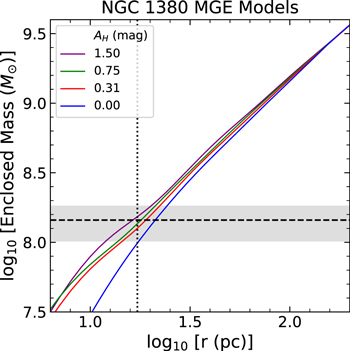
Figure 5. Plot of  vs.
vs.  in NGC 1380 for the four different MGE models, determined by calculating
  , where the v⋆,MGE values have been scaled by their respective
  values in Table 2. The resolution of the ALMA observation is denoted by the vertical dotted line and is comparable to the BH’s expected radius of influence. The BH mass determined from our fiducial model is represented by the horizontal dashed line, and the range of BH masses determined from models A–D is indicated by the gray shaded region.
Download figure:
Standard image High-resolution image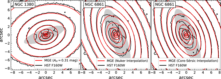
Figure 6. Isophotal contour maps of the HST F160W images of NGC 1380 and NGC 6861 displayed on an 8″ × 8″ scale. For NGC 1380 (left panel), we superpose the surface brightness contours of the intrinsic AH = 0.31 mag MGE model, while for NGC 6861 (center and right panels), we display the contours of both the Nuker and Core-Sérsic interpolation MGE models. The shapes and sizes of the central dust disks are indicated by the shaded gray ellipses.
Download figure:
Standard image High-resolution imageTable 1. H-band MGE Parameters
| k | log10 IH,k (L⊙ pc−2) |
 (arcsec) (arcsec) |

| log10 IH,k (L⊙ pc−2) |
 (arcsec) (arcsec) |

|
|---|---|---|---|---|---|---|
| (1) | (2) | (3) | (4) | (5) | (6) | (7) |
| NGC 1380 | NGC 6861 | |||||
| AH = 0.31 mag | AH = 0.00 mag (Nuker Model) | |||||
| 1 | 5.560 | 0.059 | 0.739 | 4.960 | 0.091 | 0.934 |
| 2 | 4.996 | 0.197 | 0.710 | 4.874 | 0.179 | 0.563 |
| 3 | 4.662 | 0.391 | 0.726 | 4.455 | 0.369 | 0.624 |
| 4 | 4.513 | 0.743 | 0.722 | 4.175 | 0.370 | 0.624 |
| 5 | 4.356 | 1.461 | 0.807 | 4.334 | 0.372 | 0.625 |
| 6 | 3.973 | 3.414 | 0.613 | 4.228 | 0.630 | 0.788 |
| 7 | 3.386 | 3.880 | 0.997 | 4.061 | 0.787 | 0.686 |
| 8 | 3.757 | 6.018 | 0.723 | 4.391 | 1.120 | 0.512 |
| 9 | 3.382 | 12.932 | 0.732 | 4.165 | 1.824 | 0.879 |
| 10 | 3.043 | 18.800 | 0.400 | 4.085 | 4.227 | 0.542 |
| 11 | 2.689 | 42.731 | 0.400 | 3.658 | 7.591 | 0.506 |
| 12 | 2.101 | 55.077 | 0.851 | 3.299 | 13.064 | 0.562 |
| 13 | 0.926 | 92.556 | 0.948 | 2.508 | 27.828 | 1.000 |
| 14 | ⋯ | ⋯ | ⋯ | 1.662 | 33.017 | 0.641 |
| 15 | ⋯ | ⋯ | ⋯ | 1.684 | 52.142 | 0.883 |
| 16 | ⋯ | ⋯ | ⋯ | 1.700 | 62.263 | 0.743 |
Note. NGC 1380 and NGC 6861 MGE solutions created from the combination of HST H-band images and best-fitting GALFIT Nuker models. These correspond to the AH = 0.31 mag MGE model for NGC 1380 and the Nuker interpolation MGE model for NGC 6861. As described in Section 5, these two MGEs are used in the dynamical models with the lowest χ2. The first column is the component number, the second is the central surface brightness corrected for Galactic extinction and assuming an absolute solar magnitude of M⊙,H = 3.37 mag (Willmer 2018), the third is the Gaussian standard deviation along the major axis, and the fourth is the axial ratio, which was constrained to have a minimum value of 0.400 to allow for a broader range in the inclination angle during the deprojection process. Primes indicate projected quantities.
Download table as: ASCIITypeset image
3.3. NGC 6861 Host Galaxy Models
We created our MGE models for NGC 6861 in a different fashion from our models for NGC 1380 given the differences in their dust disks. We started again by creating a J − H color map using the drizzled J- and H-band HST images of NGC 6861 to identify the pixels most affected by dust and corrected for Galactic reddening based on a foreground AH
= 0.028 (Schlafly & Finkbeiner 2011). The color map revealed the presence of a ring-like structure within the disk with a 1″ radius hole at its center, as seen in Figure 2. A measurement of the surface brightness along the major axis of the disk (shown in Figure 3) revealed a clear decrease of stellar light due to dust. This decrease is most noticeable between 1″ (the outer radius of the central hole) and 55 (the outer edge of the dust disk). The central hole is also visible in the absence of CO emission within the inner 1″ of the PVD shown in Figure 7.
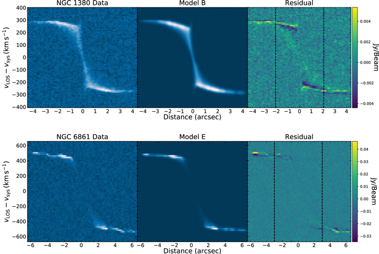
Figure 7. PVDs along the major axes of both NGC 1380 (above) and NGC 6861 (below) and their respective best-fit models. Columns show ALMA Cycle 2 CO(2–1) data (left), models (center), and (data-model) residuals (right). The PVDs were generated with a spatial extraction width equivalent to a resolution element. The black dashed lines indicate the boundaries of the elliptical fit regions along the major axes.
Download figure:
Standard image High-resolution imageGiven the lack of dynamical tracers in the central region, we wanted to test how our choice of host galaxy model impacted the inferred value of MBH. We explored systematic effects due to the choice of surface brightness model used to interpolate over the dusty region, by constructing MGEs using two different models in the correction of the H-band image for extinction: (1) a 2D Nuker model, and (2) a 2D Core-Sérsic model (Graham et al. 2003). Similar to the Nuker model, the Core-Sérsic model was designed to characterize the surface brightness profiles of ETGs. Unlike the Nuker model, however, it characterizes the outer structure of ETGs with a Sérsic profile (Sérsic 1963) and the inner structure as a power law.
To fit a Nuker model to the H-band image, we followed a process similar to that for NGC 1380, but we did not make any adjustments to the central pixels in the drizzled H-band image. We first created H-band PSF models in Tiny Tim that were dithered and drizzled in an identical fashion to the H-band image, and built a mask for foreground stars, background galaxies, and the dust disk itself. Because the J − H color map indicated a lack of color excess in the central hole, we masked the entire dust disk as seen in the J − H image, but kept the pixels within the hole to anchor the model. We fit the inner 10″ × 10″ of the H-band image with a Nuker model in GALFIT and allowed all free parameters to vary. The Nuker model parameters converged to α = 0.65, β = 1.29, γ =0.0002, and rb = 031(≈ 40 pc). Finally, we replaced pixels in the original H-band image located in the dust disk with the corresponding pixels in the Nuker model, and proceeded to fit this image with an MGE model in GALFIT without using a mask. We measured and compared this MGE model’s major axis surface brightness profile and isophotal contours to those of the H-band image in Figure 3 and Figure 6; we refer to this model as our Nuker interpolation model.
We constructed a 2D Core-Sérsic model for NGC 6861's H-band image using the imfit program (Erwin 2015) and used the same mask, model PSF, and fitting region as for our Nuker model. The parameters that characterize the Core-Sérsic model include the Sérsic index, n, break radius, rb, effective half-light radius, re, inner slope parameter, γ, and transition sharpness, α. The optimization in imfit converged on n = 7.1, rb =35(≈455 pc), re = 7
9(≈1 kpc), γ = 0.61, and α = 2.13. We replaced the pixels in the dust disk region in the original H-band image with the corresponding pixels in the Core-Sérsic model, and proceeded to fit this new image with an MGE in GALFIT. We deprojected this MGE in an identical fashion to the MGE created with the 2D Nuker model, and refer to it as our Core-Sérsic interpolation model. We extracted its major axis surface brightness profile and compared it with both the H-band image and the Nuker interpolation in Figure 3. Over the extent of the dust disk, the Core-Sérsic interpolation produces higher corrected surface brightness values than the Nuker interpolation. At the nucleus, the Nuker interpolation matches the observed central surface brightness better than the Core-Sérsic interpolation, whose innermost point slightly exceeds the observed value. A comparison with the observed H-band isophotes is shown in Figure 6. As in the case of NGC 1380, the observed isophotes became noticeably nonelliptical toward the center, although there appears to be reasonable agreement between the data and models within the central hole region. The MGE components of the Nuker interpolation are listed in Table 1, while the components of the Core-Sérsic interpolation are listed in Table 4 in the Appendix.
4. Dynamical Modeling
Our dynamical modeling formalism is a Python-based adaptation of the ALMA gas-dynamical modeling framework described by Barth et al. (2016a) and Boizelle et al. (2019), which was written in IDL and was used by those authors to measure the BH masses in NGC 1332 and NGC 3258. We describe the methods used in the Python version and the modifications that differentiate it from its IDL antecedent.
4.1. Method
Modeling the observed gas kinematics in an ALMA data cube relies on a few key steps and assumptions. First, we assume that the gas is distributed in a thin disk and is in circular rotation. A model velocity field is built on a grid that is oversampled relative to an ALMA spatial pixel by a factor of s = 3, such that each pixel is subdivided into s × s = 9 subpixels in order to model steep velocity gradients near the disk’s center. The disk’s velocity field is determined by the enclosed mass at a given radius, which consists of a central BH, the stellar mass profile of the host galaxy and a corresponding mass-to-light (M/L) ratio ϒ, and the mass profile of the gas disk. For a given disk inclination i and a major axis position angle Γ (both of which are free parameters), and an assumed (fixed) distance to the galaxy, D, we calculate the LOS projection of this velocity field as seen on the plane of the sky. The construction and geometry of the model disk are as described by Macchetto et al. (1997) and Barth et al. (2001). The LOS velocity projections are used to generate a model cube that we can compare directly to the ALMA data. For each subpixel with CO emission, we assume that the emergent line profile along the spectral dimension is intrinsically Gaussian. The Gaussian’s line centroid and line width can be calculated at each subpixel by transforming both the LOS velocity projections and a spatially uniform turbulent velocity dispersion term, σ(r) = σ0, into observed frequency units using the redshift zobs (related to the systemic velocity through vsys = czobs). The model cube must have its line profiles scaled by a model CO flux map, have each of its frequency slices convolved with the ALMA synthesized beam, and be downsampled to an appropriate resolution before being fitted to the ALMA data cube. We discuss these steps in further detail in the subsequent paragraphs and in Section 4.2.
In total, our dynamical models use a minimum of nine free parameters: the BH mass MBH, the stellar H-band M/L ratio ϒH , the disk’s dynamical center in pixels (xc, yc), the disk’s inclination and major axis position angle i and Γ, the turbulent velocity dispersion σ, the observed redshift zobs, and a flux-scaling factor F0, that correctly normalizes the model to the data.
The circular velocity vc (relative to the disk’s systemic velocity, vsys) as a function of radius is calculated as
where v⋆,MGE and vgas are the circular velocities due to the gravitational potential of the stars and the gas disk, respectively. The BH is modeled as a point mass, while the stellar and gas mass distributions are radially extended and are constructed using different methods. We modeled the stellar mass distribution using the MGE method described in Section 3.2 and Section 3.3. We deprojected the MGE under the assumptions that NGC 1380 and NGC 6861 are oblate and axisymmetric and have inclination angles of 77◦ and 73◦, respectively, based on initial gas-dynamical modeling runs. We calculated the contribution to the circular velocity from the stars in the midplane of each disk by using the mge_vcirc routine from the JamPy package in Python (Cappellari 2008) to derive a fiducial velocity profile from our MGEs. Ideally, one should match the stellar inclination angle of the MGEs to the inclination angle found for the gas disk, as mismatches between the two lead to nonequilibrium configurations for the disk. However, this matching process is difficult to implement within our framework, and we found that the differences between the stellar and gas inclination angles were small (<2°) in both NGC 1380 and NGC 6861. We will explore this aspect of the modeling process in a future work. We use ϒMGE = 1 when deriving v⋆,MGE for each galaxy. At each model iteration,  is scaled by the ratio ϒH
/ϒMGE, which scales the stellar mass profile by the free parameter ϒH
.
is scaled by the ratio ϒH
/ϒMGE, which scales the stellar mass profile by the free parameter ϒH
.
As stated earlier, Boizelle et al. (2017) created mass profiles for both gas disks by averaging the CO flux in elliptical annuli centered on the continuum peaks. They determined Mgas to be (8.4 ± 1.6) × 107 M⊙ and (25.6 ± 8.9) × 107 M⊙ for NGC 1380 and NGC 6861, respectively, but their gas mass profiles did not assume specific shapes for the mass distributions. We assumed the mass was distributed in a thin disk and numerically integrated the projected surface mass densities to determine each gas disk’s contribution to the circular velocity (vgas) using Equation (2).157 from Binney & Tremaine (2008).
We disregard the mass contribution of dark matter in our models, as the stars are expected to dominate the mass budget across the length of the circumnuclear disk. For NGC 6861, we estimated the dark matter mass within the region we fit our models (r ≈ 400 pc) by integrating the spherical cored logarithmic density profile used by Rusli et al. (2013) in their stellar-dynamical BH mass measurement. Their model suggests an enclosed dark matter mass between 106–107 M⊙, which is lower than our estimated stellar mass by two to three orders of magnitude.
The Gaussian line profiles at each point on the disk must be weighted by an observed CO flux map obtained from the ALMA observation. To create this flux map, we first visually identified channels in the data cube that contained CO emission. In these channels, we created a unique mask that separated pixels with visible emission from those without any. Spatially, each mask has the same size as a single frequency slice, with pixel values set to unity if the corresponding data cube pixel displays CO emission and zero if not. A channel that displays no emission would have a corresponding mask with all of its elements set to zero. An entire mask is 3D, with the same dimensions as the ALMA data cube. We then multiplied each slice of this mask by the corresponding slice in the ALMA data cube, and summed the products along the spectral axis. This approach produced a less noisy image of the CO flux than if we had simply summed the data cube across channels with visible emission without any masking. To deconvolve this image, we applied five iterations of the Richardson-Lucy algorithm (Richardson 1972; Lucy 1974). The deconvolution is performed with an elliptical Gaussian PSF that matches the specifications of the ALMA synthesized beam and uses the Richardson-Lucy algorithm implemented in the scikit-image package in Python (Van der Walt et al. 2014). The deconvolved image is initially constructed on the original ALMA pixel scale, with each pixel then subdivided into an s × s grid of subpixels that matches the dimensions of the oversampled model grid. The scaled and deconvolved CO flux map is normalized so that the line profiles at each subpixel element for a given original ALMA pixel have equal fluxes. Thus, if the total flux in an original ALMA pixel is F, each subpixel in the s × s grid has a flux of F/s2.
The next steps consist of rescaling the oversampled model back to the original ALMA pixel scale, convolving each frequency channel within it with the ALMA synthesized beam, and minimizing χ2 between data and model. Ideally, beam convolution should occur on the oversampled spatial grid for the highest model fidelity. However, beam convolution is the most time-consuming part of the entire modeling process and becomes prohibitively slow for oversampling factors of s > 3. Both Barth et al. (2016b) and Boizelle et al. (2019) found that modeling results do not change appreciably if the convolution step is done on the original ALMA pixel scale, so we followed the same approach. We summed each s × s group of subpixels in our oversampled model to form a single pixel on the original ALMA scale, and then convolved each frequency slice of our model with the ALMA synthesized beam, using the convolution implementation in the astropy package for Python (Astropy Collaboration et al. 2013, 2018).
4.2. Model Optimization
For a given model parameter set, we create a simulated data cube with the same spatial and spectral dimensions as the ALMA data. Therefore, our models can be fitted directly to the ALMA data cubes and can be optimized by χ2 minimization. We optimized models with the Levenberg-Marquardt algorithm (Levenberg 1944; Marquardt 1963) within the LMFIT framework (Newville et al. 2016) in Python and fitting to pixels that lay within the elliptical regions illustrated in the data moment 0 maps in Figures 8 and 9, and within the frequency channels that span the full width of the CO emission line for each pixel. We describe the fitting regions in detail in Section 4.2.2.
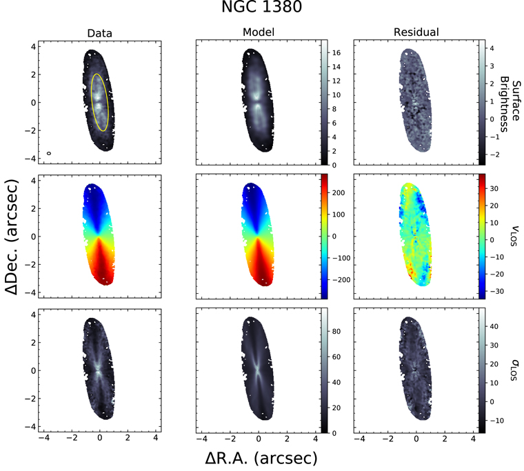
Figure 8. Moment maps for NGC 1380 constructed from the ALMA CO(2–1) data cube (left) and its fiducial model (center, model B; see Section 5.1). Shown are maps of moments 0, 1, and 2, corresponding to surface brightness, line-of-sight velocity vLOS, and turbulent velocity dispersion σLOS. The units for the surface brightness map are mJy km s−1 pixel−1, and the units for the vLOS and σLOS maps are km s−1. The systemic velocity of 1854 km s−1 estimated from our dynamical models has been removed from vLOS. Maps of (data-model) residuals are shown in the rightmost column. While the line profile fits have been determined at each pixel of the full disk, the elliptical fitting region used in calculating χ2 is denoted in the top-left panel with a yellow ellipse. The synthesized beam is represented by an open ellipse in the bottom-left corner of the same image.
Download figure:
Standard image High-resolution image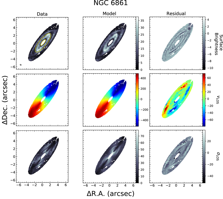
Figure 9. Moment maps for NGC 6861 constructed from the ALMA CO(2–1) data cube (left) and our model E (center). Shown are maps of moments 0, 1, and 2 corresponding to surface brightness, line-of-sight velocity vLOS, and turbulent velocity dispersion σLOS. The units for the surface brightness map are mJy km s−1 pixel−1, and the units for the vLOS and σLOS maps are kilometers per second. The systemic velocity of 2796 km s−1 estimated from our dynamical models has been removed from vLOS. A (data-model) residual is shown in the rightmost column. While the line profile fits have been determined at each pixel of the full disk, the annular fitting region used in calculating χ2 is denoted in the top-left panel with a yellow annulus. The synthesized beam is represented by an open ellipse in the bottom-left corner of the same panel.
Download figure:
Standard image High-resolution image4.2.1. Noise Model
In order to calculate χ2 and assess the goodness-of-fit of our models to the ALMA data, we require an estimate of the flux uncertainty at each data pixel. The most straightforward approach here would be to calculate the standard deviation of pixel values in emission-line-free regions of the data cube. However, the background noise in ALMA data cubes is correlated on scales comparable to the synthesized beam in each frequency channel. This correlation prevents the determination of a meaningful χ2 value without appropriate adjustments. Ideally, one would calculate a covariance matrix accounting for these correlations to compute χ2, but such an approach would be computationally expensive and challenging to implement. Barth et al. (2016b) and Boizelle et al. (2019) adopted the simpler approach of rebinning the data by block-averaging over m × m pixel blocks within each frequency channel, where the value of m was the approximate number of pixels across the width of the synthesized beam. Their method creates a data cube with a scale of approximately one rebinned pixel per synthesized beam, and mitigates the noise correlation among neighboring pixels. They then measured the standard deviation of emission-free pixels in the rebinned data cube to produce a unique value of flux uncertainty for each frequency channel, and similarly rebinned their models to compute χ2 on the block-averaged scale.
We also incorporated the effects of the ALMA primary beam on the background noise level. Prior to primary beam correction, the noise level in an ALMA data cube is spatially uniform, but post-correction it increases with distance from the phase center. Dynamical models are created and fitted to data cubes that have been corrected for the primary beam attenuation, so we incorporated this spatial modification into our noise model. As part of the ALMA data reduction process, a primary beam cube is generated along with the beam-corrected data cube. Multiplying the corresponding slices of these cubes together generates an uncorrected version of the data in which the background noise is spatially uniform. At this step, we block-average the data to roughly the size of the synthesized beam, using 7 × 7 pixel blocks for the NGC 1380 data cube and 4 × 4 pixel blocks for the NGC 6861 data cube. Once the data have been rebinned, we measure the standard deviations of pixel values in blank regions of each frequency channel, and populate an array having the spatial dimensions of a block-averaged image with the value of the standard deviation at each element. To replicate the spatial modification of the noise in each channel, we block-averaged the primary beam cubes over the same pixel blocks as was done for the data and divided the block-averaged array of standard deviations by the block-averaged primary beam cube at the same frequency. In essence, we create a block-averaged noise cube that captures both the spatial and frequency dependence of the noise, which we use to compute χ2. This approach differs from previous methods where the given background noise is assumed to be spatially uniform across a given frequency slice (Barth et al. 2016b; Boizelle et al. 2019).
Although our noise model is designed to represent the rms noise in emission-line-free regions of each frequency channel of the data cube, an additional complication is that the mean background level can be slightly offset from zero (e.g., as a residual of imperfect passband calibration or continuum subtraction). If this is the case, the line-free regions of a cube will indirectly contribute to elevated χ2 values for model fits. For both galaxies, we find roughly equal number of channels having positive and negative mean background levels, with typical magnitudes ∼10% of the respective per-channel rms noise levels. As a simple test, we empirically measured the mean background level in each frequency channel included in our fit and added this value into the corresponding channels in our synthetic model cubes. We found that our values of reduced χ2 were smaller by about ∼1% with this adjustment, and hence the impact of these background levels can be regarded as minimal.
4.2.2. Fit Regions
We computed χ2 over elliptical fitting regions to assess the goodness-of-fit of our dynamical models. These elliptical fitting regions were centered on the disk centers and used the axial ratios and major axis position angles of the gas disks, as measured by Boizelle et al. (2017). The size of the fitting region can influence the inferred value of MBH. While fitting models to the entire disk uses all of the available data, the majority of pixels in the fit are at radii much greater than the BH’s radius of influence. In this regime, the uncertainty in the stellar mass profile accounts for a large portion of the error budget, and model fits can lead to tight statistical constraints on both ϒH and MBH. If the assumed and intrinsic shapes of the stellar mass profile are discrepant, full-disk fits can force MBH to an inaccurate, but highly precise value. Alternatively, fitting to smaller regions can mitigate effects from discrepancies in the stellar mass profile because the BH mass represents a larger fraction of the total enclosed mass. Smaller fit regions can also limit systematic effects due to the structural mismatch of a thin disk model with a mildly warped disk. We discuss our selected fitting regions for NGC 1380 and NGC 6861 below.
For NGC 1380, we initially created an ellipse centered on the disk center with an axial ratio of q = 0.27, and a position angle of Γ = 187° based on results from Boizelle et al. (2017). For our fiducial dynamical model, we chose to fit within an ellipse that encompassed the inner half of the CO disk in order to limit the sensitivity of our dynamical models to the shape of the stellar mass profile and the disk’s slightly warped structure. We also modified the size of this ellipse to see how the choice of fit region affected the inferred value of MBH in Section 5.2. Our final fitting ellipse has a semimajor axis of a = 205 and a semiminor axis of b = 0
55. This ellipse was used across 62 consecutive frequency channels that spanned the full width of the visible CO emission in the data and can be seen in Figure 8. On the final rebinned scale, this choice of spatial and spectral regions resulted in 61 block-averaged pixels over 62 frequency channels for a total of 3782 data points used to calculate χ2.
For NGC 6861, we initially followed the same procedure, starting with the values of q = 0.32 and Γ = 141° found by Boizelle et al. (2017). However, the disk structure in NGC 6861 is more complicated than in NGC 1380. The NGC 6861 gas disk contains a central hole that is ∼1″ in radius along the major axis. Thus, the innermost CO emission is at a radius that is three times larger than the BH’s estimated radius of influence. Additionally, the presence of rings and spiral-like substructure can be seen toward the edge of the disk. Fitting models to the entire disk led to reduced χ2 values between 2.5 and 3, as the thin disk models struggled to reproduce kinematic features in the outer disk. The inner half of the gas disk shows the most regularity in its structure, and we found that fitting dynamical models in this region led to lower reduced χ2 values and better overall fits to the data. Therefore, we created an elliptical fitting region with dimensions a = 3″ and b = 096, as seen in Figure 9. In order to prevent pixels within the hole from contributing to the fit, we masked out a 1″ ellipse with the same axial ratio (q = 0.32) at the center of our fitting region, which yielded our final annular fitting region. Along the spectral axis, we fit across 52 frequency channels that extended slightly beyond the channels with visible emission. On the final rebinned scale, with 75 rebinned pixels per channel, we included a total of 3900 data points in the fit.
5. Results
5.1. NGC 1380 Modeling Results
We present results for four models for NGC 1380, which we refer to as models A, B, C, and D in Table 2. The key difference among them is the input host galaxy circular velocity profile, based on one of the four MGE models described in Section 3.2, which accounted for four fiducial values of central dust extinction (AH = 0.00, 0.31, 0.75, and 1.50 mag for models A, B, C, and D, respectively). These dynamical models use a uniform turbulent velocity dispersion across the entire disk and are optimized over the elliptical region described in Section 4.2.2.
Table 2. Dynamical Modeling Results
| Model | MGE | MBH | ϒH | i | Γ | σ0 | xc | yc | vsys | F0 |

| |
|---|---|---|---|---|---|---|---|---|---|---|---|---|
| (M⊙/L⊙) | (°) | (°) | (km s−1) | (arcsec) | (arcsec) | (km s−1) | ||||||
| NGC 1380 | ||||||||||||
| (AH mag) | (108 M⊙) | |||||||||||
| A | 0.00 | 1.85 | 1.33 | 76.9 | 187.1 | 10.8 | 0.016 | 0.013 | 1853.83 | 0.99 | 1.544 | |
| B | 0.31 | 1.47 | 1.42 | 76.9 | 187.2 | 10.5 | 0.017 | 0.013 | 1853.86 | 0.99 | 1.525 | |
| (0.02) | (0.003) | (0.04) | (0.04) | (0.13) | (0.001) | (0.001) | (0.15) | (0.003) | ||||
| C | 0.75 | 1.27 | 1.36 | 76.9 | 187.2 | 10.5 | 0.017 | 0.013 | 1853.86 | 0.99 | 1.545 | |
| D | 1.50 | 1.02 | 1.30 | 76.8 | 187.2 | 10.5 | 0.017 | 0.013 | 1853.88 | 0.99 | 1.563 | |
| NGC 6861 | ||||||||||||
| (Nuclear Profile) | (109 M⊙) | |||||||||||
| E | Nuker | 1.13 | 2.52 | 72.7 | 142.5 | 7.2 | 0.057 | 0.038 | 2795.63 | 1.03 | 1.987 | |
| (0.04) | (0.01) | (0.07) | (0.05) | (0.29) | (0.002) | (0.002) | (0.29) | (0.006) | ||||
| F | Core-Sérsic | 2.89 | 2.14 | 73.6 | 142.6 | 7.4 | 0.049 | 0.046 | 2795.65 | 1.04 | 2.004 | |
Note. Best-fit parameter values obtained by fitting thin disk dynamical models to the NGC 1380 and NGC 6861 CO(2–1) data cubes. We derive 1σ statistical uncertainties for the parameters of fiducial models B and E, based on a Monte Carlo resampling procedure described in Section 5.1 and list them under the results for models B and E. These models have 3773 and 3891 degrees of freedom, respectively. The major axis PA, Γ, is measured east of north for the receding side of the disk. The disk dynamical center, (xc, yc) is measured in arcsecond offsets from the nuclear continuum centroids for NGC 1380 and NGC 6861 determined in Boizelle et al. (2017). The observed redshift, zobs, is used in our dynamical models as a proxy for the systemic velocity of the disk, vsys, in the barycentric frame via the relation: vsys = czobs and is used to translate the model velocities to observed frequency units.
Download table as: ASCIITypeset image
Models A–D yield best-fit values of MBH in the range of (1.02–1.85) × 108
M⊙, ϒH
between 1.30 and 1.42, and a range in reduced χ2
 between 1.525 and 1.563 over 3773 degrees of freedom. Our measured range of ϒH
is slightly above the predictions made from single stellar population (SSP) models (Vazdekis et al. 2010) that assume either a Kroupa (2001) or Chabrier (2003) initial-mass function (IMF) and is lower than predictions made with a Salpeter (1955) IMF. These SSP models assume an old stellar population (10–14 Gyr) and solar metallicity, which are consistent with 2D IMF analyses of NGC 1380 by Martín-Navarro et al. (2019). As seen in Table 2, all other free parameters remained virtually unchanged among the different dynamical models. We discuss the interplay between MBH and ϒH
in Section 6.1.
between 1.525 and 1.563 over 3773 degrees of freedom. Our measured range of ϒH
is slightly above the predictions made from single stellar population (SSP) models (Vazdekis et al. 2010) that assume either a Kroupa (2001) or Chabrier (2003) initial-mass function (IMF) and is lower than predictions made with a Salpeter (1955) IMF. These SSP models assume an old stellar population (10–14 Gyr) and solar metallicity, which are consistent with 2D IMF analyses of NGC 1380 by Martín-Navarro et al. (2019). As seen in Table 2, all other free parameters remained virtually unchanged among the different dynamical models. We discuss the interplay between MBH and ϒH
in Section 6.1.
The major axis PVD, moment maps, and example line profiles for our best-fit model (model B) for NGC 1380 are presented and compared with the ALMA data in Figures 7, 8, and 10. The moment maps and PVD reveal that the data and model are in good agreement over a majority of the disk, although a mismatch in the observed surface brightness is seen in both the moment 0 (surface brightness) map and in the structure of the PVD, especially within the innermost ∼05. Moment 1 (vLOS) maps show that data and model velocity fields are also in good agreement, although differences of ∼30 km s−1 are noticeable toward the disk edge, outside the fit region, and at the disk center, where the impact of beam-smearing is most severe. Most likely, these differences are a result of the differences between the model and intrinsic stellar velocity profiles. The extracted line profiles of the block-averaged data and best-fit model highlight our models’ ability to reproduce the observed shapes of the line profiles, even when they display asymmetric structure.
To determine the statistical uncertainties of the free parameters, we performed a Monte Carlo simulation for model B. We created 150 realizations of the best-fit model by adding noise to each pixel of the model cube. The value of the noise at each pixel was determined by choosing a random value drawn from a Gaussian distribution with a standard deviation equal to the value of the corresponding pixel in the noise cube described in Section 4.2.1. We re-fit to each noise-added model realization using the values found in Table 2 as initial guesses; the standard deviation of each recovered parameter was identified as the 1σ uncertainty. For MBH, we found a tight distribution centered at our initial guess of MBH = 1.47 × 10⁸ M⊙ with a standard deviation of 2 × 10⁶ M⊙, or 1.4% of the mean. The statistical uncertainties for the free parameters are listed under model B’s best-fit values in Table 2. Based on other Monte Carlo simulations we ran, these statistical uncertainties are representative of those for models A, C, and D.
5.2. Error Budget for NGC 1380
While the statistical uncertainties from our Monte Carlo simulation are small, there are several other sources of uncertainty that stem from the choices we made when building our dynamical models. Thus, we conducted numerous tests to determine the impact these choices had on the value of MBH.
Dust extinction: The value of MBH in our model optimizations is highly sensitive to the choice of MGE model. Using the initial, dust-masked MGE, our models converge on MBH = 1.85 × 10⁸
M⊙. As we increase the central extinction from AH
= 0.00 mag to AH
= 0.31 mag, corresponding to a loss of 25% of the total stellar light behind the dusty disk, MBH decreased to 1.47 × 10⁸
M⊙, representing a ∼20% decrease from the initial fit. This particular model also shows a decrease in the resultant  , as model A with the initial MGE returns
  , while model B with AH
= 0.31 mag yields
, while model B with AH
= 0.31 mag yields  . Increasing the extinction further to AH
= 0.75 mag and AH
= 1.50 mag further decreases MBH, as models C and D converge to values of 1.27 × 10⁸
M⊙ and 1.02 × 10⁸
M⊙, i.e., ∼31% and ∼45% decreases from the model A value, respectively. However, both models C and D result in higher
. Increasing the extinction further to AH
= 0.75 mag and AH
= 1.50 mag further decreases MBH, as models C and D converge to values of 1.27 × 10⁸
M⊙ and 1.02 × 10⁸
M⊙, i.e., ∼31% and ∼45% decreases from the model A value, respectively. However, both models C and D result in higher  values.
We chose the AH = 0.31 mag MGE model (model B) to use as our fiducial model for a number of reasons. First, this MGE model accounts for the impact of dust extinction, whereas the initial MGE simply masks dust out. Next, the dynamical model that uses the AH = 0.31 mag MGE has the lowest value of χ2 out of all of our models, signifying the best overall match to the ALMA data. Lastly, extracting the major axis surface brightness profile from this MGE model reveals that it most closely resembles our surface brightness profile after correction for the low-extinction branch of the reddening curve shown in Figure 3. Therefore, for all of the remaining systematic tests, we use the AH = 0.31 mag MGE as our host galaxy model.
Radial motion: Although there is no evidence of strong deviations from circular motion in the NGC 1380 gas disk, we constructed a simple model that allows for radial motion in our dynamical models. We followed an approach similar to Boizelle et al. (2019) and Cohn et al. (2021) and added a radially inward velocity term to our dynamical models. We included an additional free parameter, α, which lies in the range [0, 1] and controls the balance between pure rotational (α = 1) and radially inflowing (α = 0) motion. Mathematically, we defined α to be the ratio between the rotational velocity, vrot, and the ideal circular velocity in our model grid (i.e., α = vrot/vc
). We defined the relationship between α, radial inflow velocity, and the ideal circular velocity as  . Thus, when α = 1, our model velocities are circular, and when α = 0, the velocities are radially inflowing at the ideal freefall speed of a test particle falling in from infinity. We projected the radial velocity component along the LOS, and added it linearly to the projected LOS rotation velocity at each pixel in our model grid. Upon optimizing, we found that the models strongly favored pure rotation, with a best-fitting value of α = 1. This model converged on MBH = 1.47 × 10⁸
M⊙, leaving the results found for the fiducial model unchanged.
. Thus, when α = 1, our model velocities are circular, and when α = 0, the velocities are radially inflowing at the ideal freefall speed of a test particle falling in from infinity. We projected the radial velocity component along the LOS, and added it linearly to the projected LOS rotation velocity at each pixel in our model grid. Upon optimizing, we found that the models strongly favored pure rotation, with a best-fitting value of α = 1. This model converged on MBH = 1.47 × 10⁸
M⊙, leaving the results found for the fiducial model unchanged.
Turbulent velocity dispersion: The ratio of the turbulent velocity dispersion to the rotational velocity (σ/vrot) determines if the disk can be treated as dynamically cold (where  , or if dynamical pressure effects from turbulence must be accounted for. By using our AH
= 0.31 mag MGE model, our radial gas mass profile, the fiducial BH mass, and our best-fit value of σ0 = 10.5 km s−1, we find a maximum value of σ0/vc = 0.05 (where we have set vrot = vc, the ideal circular velocity) at about r = 50 pc, indicating that treating the disk as dynamically cold and neglecting dynamical pressure effects are justified. Nevertheless, a spatially uniform turbulent velocity dispersion term might be insufficient to characterize possible variations in turbulence across the entire disk. Therefore, in addition to using a spatially uniform gas turbulent velocity dispersion term, σ(r) = σ0, we also tried incorporating a Gaussian turbulent velocity dispersion profile
, or if dynamical pressure effects from turbulence must be accounted for. By using our AH
= 0.31 mag MGE model, our radial gas mass profile, the fiducial BH mass, and our best-fit value of σ0 = 10.5 km s−1, we find a maximum value of σ0/vc = 0.05 (where we have set vrot = vc, the ideal circular velocity) at about r = 50 pc, indicating that treating the disk as dynamically cold and neglecting dynamical pressure effects are justified. Nevertheless, a spatially uniform turbulent velocity dispersion term might be insufficient to characterize possible variations in turbulence across the entire disk. Therefore, in addition to using a spatially uniform gas turbulent velocity dispersion term, σ(r) = σ0, we also tried incorporating a Gaussian turbulent velocity dispersion profile ![$\sigma {(r)={\sigma }_{0}+{\sigma }_{1}\exp [-(r-{r}_{0})}^{2}/2{\mu }^{2}]$](https://content.cld.iop.org/journals/0004-637X/934/2/162/revision1/apjac7a38ieqn22.gif) into our fiducial model. This profile adds three free parameters and allows for more flexibility in characterizing the overall velocity dispersion. However, the model is not physically motivated, and is used here as a simple tool for exploring possible variations in σ(r). The preferred turbulent velocity dispersion parameters of σ0 = 10.6 km s−1, σ1 = 0.21 km s−1, r0 = 0.06 pc, and μ =0.02 pc yield a turbulent velocity dispersion profile that is dominated by the spatially uniform term of 10.6 km s−1, and is nearly identical to the fiducial model’s spatially uniform σ0 = 10.5 km s−1. The modified model yields MBH = 1.47 ×10⁸
M⊙ and
into our fiducial model. This profile adds three free parameters and allows for more flexibility in characterizing the overall velocity dispersion. However, the model is not physically motivated, and is used here as a simple tool for exploring possible variations in σ(r). The preferred turbulent velocity dispersion parameters of σ0 = 10.6 km s−1, σ1 = 0.21 km s−1, r0 = 0.06 pc, and μ =0.02 pc yield a turbulent velocity dispersion profile that is dominated by the spatially uniform term of 10.6 km s−1, and is nearly identical to the fiducial model’s spatially uniform σ0 = 10.5 km s−1. The modified model yields MBH = 1.47 ×10⁸
M⊙ and  , demonstrating almost no effect on the results of the fiducial model.
Fit region: We tested the sensitivity of MBH to the fit regions of the dynamical models by making two separate adjustments to the spatial fitting ellipse described in Section 4.2.2 and used to calculate χ2. The first adjustment was expanding the fitting ellipse to cover the entirety of the gas disk, with semimajor axis length 41 and semiminor axis length 1″. For this fitting ellipse, the models converged on MBH = 1.63 × 10⁸
M⊙, an increase of 10.9% from the fiducial model, and
 . This larger fitting ellipse includes nearly four times as many data points, but a majority of points are at radii where the extended stellar mass distribution dominates the total enclosed mass.
Our second adjustment was reducing the fitting ellipse to fit only the inner third of the disk, with semimajor and semiminor axis lengths of 137 and 0
33. The resultant value of MBH was 1.52 × 10⁸
M⊙, an increase of 3.4% relative to our fiducial model, with
 . On this scale, the fit contains a higher fraction of data points that display unresolved gas kinematics, particularly along the disk’s minor axis, where beam-smearing effects are more severe.
Pixel oversampling: Other molecular gas-dynamical studies such as Barth et al. (2016a) have found that MBH is relatively insensitive to the choice of pixel oversampling factor, s. We tested our own dynamical models with oversampling factors of s = 1 and s = 4. For s = 1, the result was MBH = 1.45 ×10⁸
M⊙, a decrease of 1.4% relative to model B, with a higher  of 1.543, as expected for no pixel oversampling. At s = 4, the resulting MBH was 1.47 × 10⁸
M⊙, identical to our fiducial model result, with a slightly improved
of 1.543, as expected for no pixel oversampling. At s = 4, the resulting MBH was 1.47 × 10⁸
M⊙, identical to our fiducial model result, with a slightly improved  of 1.524. These results show that MBH has little sensitivity to the choice of s, even in the no-oversampling case of s = 1.
Gas mass: We performed two tests to observe the dependence of MBH on the inclusion or exclusion of the gas disk’s contribution to the mass model. First, we optimized a dynamical model that did not include the circular velocity contribution from the gas disk, which was derived from the mass surface densities in Boizelle et al. (2017), but otherwise used the same inputs as model B. Without this contribution, the model converged upon MBH = 1.43 × 10⁸
M⊙, a decrease of 2.7%, and the same  as our fiducial model. In addition, we rescaled the gas mass surface densities to the lower value implied by a CO(2–1)/CO(1–0) intensity ratio ≈0.9 (see Section 2.2.2) and reoptimized our dynamical model with this adjusted circular velocity contribution. With this adjustment, our model converged upon MBH = 1.45 × 10⁸
M⊙, and an identical
as our fiducial model. In addition, we rescaled the gas mass surface densities to the lower value implied by a CO(2–1)/CO(1–0) intensity ratio ≈0.9 (see Section 2.2.2) and reoptimized our dynamical model with this adjusted circular velocity contribution. With this adjustment, our model converged upon MBH = 1.45 × 10⁸
M⊙, and an identical  . These results suggests the inclusion or exclusion of the gas component in models can be important in percent-level precision BH mass measurements. However, for our measurements, it is a relatively minor contribution to the error budget in comparison to that of the dust extinction.
Unresolved active calactic nucleus emission: Given that there is evidence of a weak AGN in NGC 1380, we explored the possibility that our MGEs could be incorporating the light from this AGN in addition to the stars. As a test, we removed the innermost component (FWHM = 014 = 11.5 pc) of the AH
= 0.31 mag MGE model, and deprojected the remaining components. Using this altered MGE model, the BH mass rose to MBH = 2.04 × 10⁸
M⊙, an increase of 38.7% from the fiducial BH mass (1.47 × 10⁸
M⊙) found when we included the innermost component, but the reduced χ2 value also rose to 1.528, indicating a poorer fit to the data. If we deproject this innermost component individually, and assume it is composed entirely of starlight, the corresponding stellar mass is 0.59 × 10⁸
M⊙ (assuming ϒH
= 1.42), which is slightly higher (by 2 × 10⁶
M⊙) than the difference in BH mass. While it is difficult to determine the amount of AGN light in the innermost MGE component, given that the increase in BH mass between the two dynamical models is commensurate with the decrease in assumed stellar masses, this test shows that the BH and stellar mass of the innermost component are degenerate.
The large range of MBH found in Table 2 and the sensitivity tests performed above show that the systematic error is dominated by the uncertainties associated with the host galaxy models. Specifically, these uncertainties are associated with the amount of stellar mass, which changes depending on the assumed dust extinction and/or the presence or absence of an AGN contributing to the central host galaxy light, as shown when we removed the innermost component of our MGE. We chose model B as our fiducial model for the reasons described in Section 5.2 and treat the ΔMBH between its MBH value of 1.47 × 10⁸ M⊙ and the maximum (1.85 × 10⁸ M⊙) and minimum MBH (1.02 × 10⁸ M⊙) values found in Table 2 as a rough estimate of the uncertainty due to the dust correction. These maximum and minimum values are about 26% larger and 31% smaller than the fiducial MBH value, respectively.
It is clear that the systematic uncertainties exceed the statistical uncertainty (≈1%) and the uncertainty associated with the distance to the galaxy (≈ 8%; Tonry et al. 2001). Considering that the uncertainties from the dust correction and the host galaxy mass modeling dominate the total systematic uncertainty, we adopt the BH mass of 1.47 × 10⁸ M⊙ from our fiducial model and the aforementioned uncertainties as our estimate for MBH. Therefore, the expected range of MBH in NGC 1380 is (1.02–2.04) × 108 M⊙.
5.3. NGC 6861 Modeling Results
We optimized two different dynamical models for NGC 6861, which we refer to as models E and F in Table 2. The difference between them is the input stellar circular velocity profile, based on one of the two NGC 6861 MGE models described in Section 3.3 that model the nuclear region in the H-band image with either a Nuker (E) or Core-Sérsic (F) model. These two dynamical models used a uniform turbulent velocity dispersion across the entire disk and are optimized over the annular region described in Section 4.2.2.
Model E converges on MBH = 1.13 × 10⁹
M⊙ and ϒH
= 2.52 with  , while model F returns values of MBH =2.89 × 10⁹
M⊙ and ϒH
= 2.14 with
, while model F returns values of MBH =2.89 × 10⁹
M⊙ and ϒH
= 2.14 with  . The ϒH
values are higher than the ranges predicted by the SSP models of Vazdekis et al. (2010). Similarly, the range of ϒI
= (5.7–6.3) determined observationally by Rusli et al. (2013) is higher than SSP model predictions. All other free parameters remain consistent between the two models, although the inclination angle i slightly increases from 72
. The ϒH
values are higher than the ranges predicted by the SSP models of Vazdekis et al. (2010). Similarly, the range of ϒI
= (5.7–6.3) determined observationally by Rusli et al. (2013) is higher than SSP model predictions. All other free parameters remain consistent between the two models, although the inclination angle i slightly increases from 727 to 73
6 from model E to F.
We created moment maps and a major axis PVD, and extracted line profiles for model E to compare with the ALMA data. The residuals between the data and model vLOS maps show that our thin disk model emulates the data’s observed vLOS well within our designated fitting region, but discrepancies in excess of ∼60 km s−1 are seen at larger radii. These discrepancies highlight kinematic substructure within the disk at these larger radii that our models are unable to reproduce, although given that the maximum value of σ0/vc across the NGC 6861 disk is ∼ 0.02, our treatment of the disk as dynamically cold is justified. The PVD also shows discrepancies along the major axis, as structural differences between the data and model PVDs are prevalent at radii larger than ∼3″, which corresponds to the semimajor axis of our elliptical fitting region. The extracted line profiles in Figure 10 show that our models are able to reproduce the observed line profile shapes well, although slight inconsistencies in the peak amplitude, in terms of both overall height and velocity channel, are evident in some spectra.
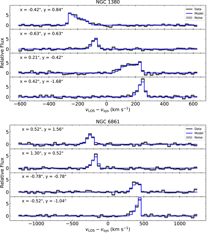
Figure 10. Representative line profiles of NGC 1380 (above) and NGC 6861 (below) measured by extracting single pixel cuts through our data, model, and noise cubes at four locations. The model line profiles are assumed to be intrinsically Gaussian at the subpixel level, with the asymmetric structure coming from beam-smearing. The noise band represents values in the range of data ± 1σ. These line profiles were extracted from the cubes on the final scale of 1 block-averaged pixel per synthesized beam. The x and y labels indicate the pixel locations in terms of offsets in arcseconds from the disk dynamical centers, which are given in Table 2.
Download figure:
Standard image High-resolution imageWe conducted Monte Carlo simulations to estimate fitting uncertainties for both model E and F as we did for model B. We generated 150 realizations of each model cube by adding noise to each pixel as described in Section 5.1. For model E, we found a distribution centered at its best-fit MBH value of 1.13 × 10⁹ M⊙ with a standard deviation of 4 × 10⁷ M⊙, or 1.4% of MBH. Model F’s Monte Carlo simulation was centered at MBH = 2.89 × 10⁹ M⊙ and also had a standard deviation of 4 × 10⁷ M⊙, or 3.5% of MBH. We chose to use the standard deviations of each of the free parameters from model E as representative of statistical uncertainties associated with these values and list them in Table 2.
The Monte Carlo simulations show that the statistical model-fitting uncertainties are significantly smaller than the systematic uncertainty associated with our choice of host galaxy model, which return values of MBH that are different by a factor of ∼ 3. Because of this large difference in MBH between models E and F, we did not perform extensive systematic tests on these models as we did for model B in Section 5.2, as the uncertainty associated with our choice of host galaxy model dominates the total error budget.
To determine a lower limit on MBH, we adjusted the central flux in NGC 6861's H-band image in the same manner as was done for NGC 1380's H-band image in Section 3.2. We corrected our Nuker interpolation MGE model under the assumption that the disk resides in the midplane of the galaxy and that only the starlight originating from behind the dust disk experiences any extinction. Our modified Nuker interpolation model explored the extreme limit where AH
= ∞ , signifying that all of the light behind the disk is lost, and raising the innermost value of the major axis surface brightness profile by 0.75 mag  . Even with this maximally peaked surface brightness model, the value of MBH was nonzero and converged on 9.7 × 10⁷
M⊙, which serves as our measurement’s lower limit. We emphasize that even with the assumption that the central region of NGC 6861 is optically thick (which is highly unlikely given the J − H color map) and the absence of dynamical information within the inner 1″, our dynamical models still require a central compact mass to reproduce the observations.
. Even with this maximally peaked surface brightness model, the value of MBH was nonzero and converged on 9.7 × 10⁷
M⊙, which serves as our measurement’s lower limit. We emphasize that even with the assumption that the central region of NGC 6861 is optically thick (which is highly unlikely given the J − H color map) and the absence of dynamical information within the inner 1″, our dynamical models still require a central compact mass to reproduce the observations.
6. Discussion
Our molecular gas-dynamical measurements are the first and second attempts to determine the masses of the central BHs in NGC 1380 and NGC 6861, respectively. For each galaxy, the presence of dust limits the measurement precision on MBH. In NGC 1380, we find MBH = 1.47 × 10⁸ with an uncertainty of ∼40%, which is dominated largely by the dust corrections. The measurement precision for NGC 6861's BH is even more limited due to the lack of dynamical tracers within the BH’s sphere of influence, as the resulting values of MBH differ by a factor of ∼3 depending on the model used for the host galaxy. Below, we discuss the importance of resolving the BH’s sphere of influence and accounting for the presence of dust in both galaxies. We also discuss how parameter degeneracies emerge within our models from these factors, and we compare our measured MBH values to predictions from the BH–host galaxy scaling relations given by Kormendy & Ho (2013).
6.1. The BH Sphere of Influence
The precision of a BH mass measurement is highly dependent on how well the observations resolve the radius of the BH’s dynamical sphere of influence, rg
. Within rg
, the central BH is the dominant contributor to the total gravitational potential. If rg
is unresolved, then the measured value of MBH depends heavily on the accuracy of the assumed host galaxy model, and dynamical models are susceptible to parameter degeneracies. For each galaxy, we estimated rg
in two distinct ways. The first was to determine the radius where MBH is equal to the enclosed stellar mass, and the second was to calculate  using our measured values of MBH and known literature values of σ⋆ for both galaxies.
For NGC 1380, we used the best-fit value of MBH = 1.47 ×10⁸
M⊙ from our fiducial model to determine rg
. The radius where the enclosed stellar mass (derived from the MGE used in the fiducial model) equaled MBH was rg
= 18 pc (022), which is nearly identical to our average beam size of 0
21. If we instead calculate rg
as
 , using the average value of σ⋆ = 215 km s−1 from Hyperleda (Makarov et al. 2014), we find rg
= 14 pc (0
, using the average value of σ⋆ = 215 km s−1 from Hyperleda (Makarov et al. 2014), we find rg
= 14 pc (017). We display both the total enclosed mass profile and the separate contributions from each component to our dynamical model in Figure 11. These estimates demonstrate it is likely that the observations only marginally resolve rg
.
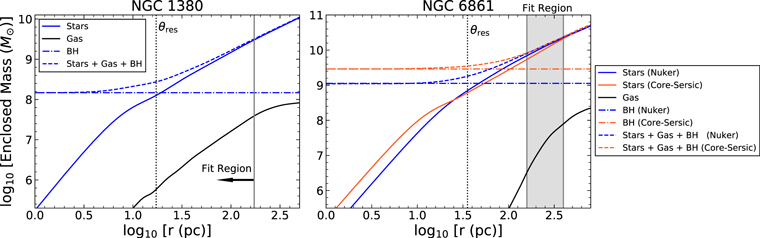
Figure 11. Enclosed mass profiles as a function of radius used in the dynamical modeling of NGC 1380 (left) and NGC 6861 (right). We show the mass contributions from the stars, gas, and BH, as well as the sums of their masses. For NGC 1380, we display the stellar mass profile associated with the AH
= 0.31 mag MGE used in our fiducial model. For NGC 6861, the enclosed mass profiles associated with our Nuker interpolation MGE model fit are shown in blue, while those associated with our Core-Sérsic interpolation MGE model are shown in orange. The gray shaded region indicates the radii over which dynamical modeling fits were performed along the major axis. The dotted lines correspond to the 021 and 0
28 resolutions of the NGC 1380 and NGC 6861 Cycle 2 observations, respectively.
Download figure:
Standard image High-resolution imageWhile there is evidence of a slight central upturn in gas velocity within the innermost ∼02 of NGC 1380, given that the observations do not fully resolve rg
, it is unsurprising that our measurement of MBH carries a large uncertainty of about 40% (dominated mostly by the uncertainties from the dust correction and host galaxy modeling), and that our dynamical models have a degeneracy between BH and stellar mass. In essence, our dynamical models’ ability to distinguish their separate contributions is severely limited when rg
is not fully resolved. This limitation was demonstrated by our test removal of the innermost component of the host galaxy MGE model, as the increase in MBH was commensurate with the decrease in stellar mass. While the total enclosed mass is well-constrained at large radii, the mass contributions from the BH and the stars within the central regions are not. This degeneracy is highlighted in Figure 5, which shows stellar mass versus radius for our dust-masked and dust-corrected host galaxy models. With each progressive increase in assumed dust extinction, the stellar mass becomes a larger fraction of the total enclosed mass. While the differences in our stellar mass profiles are minimal at radii greater than ∼100 pc, it is their differences within the innermost ∼30 pc that lead to decreases in MBH and variations in ϒH
. Given that the total enclosed mass is tightly constrained by the well-resolved kinematics at large radii, the cuspier surface brightness models require smaller MBH values.
For NGC 6861, we estimated rg
using the best-fit values of MBH from both model E and model F. The BH mass and the enclosed stellar mass were equal at 47 pc (036) if we adopt the stellar mass profile from model E, and at 94 pc (0
72) for model F. If we instead use the velocity dispersion of σ⋆ = 389 km s−1 from Rusli et al. (2013), we obtain rg
= 32 pc (0
25) when adopting the best-fit MBH from model E and 82 pc (0
63) from model F. Considering that the average ALMA beam size for the NGC 6861 data is 0
28, these estimates suggest that rg
would be resolved in NGC 6861.
Despite having observations that could in principle resolve rg if the gas disk extended to the center in NGC 6861, the lack of CO emission within the innermost ∼1″ precludes a high-precision BH mass measurement, as our two dynamical models found BH mass values that differed by a factor of ∼3 and were degenerate with ϒH . We attribute this large disparity to the central hole, and to the differences between our Nuker and Core-Sérsic interpolation MGE models in the dust-affected regions. These differences, especially in the slope of the surface brightness profile, led to distinct ϒH values in the dynamical models. Additionally, the dearth of CO emission within the innermost 1″ meant that model fits were optimized over pixels that were more sensitive to differences in the stellar mass distribution. Figure 11 shows the separate and combined enclosed mass profiles of the stars, gas, and BH for each host galaxy model used. Using these mass profiles, we determined the total enclosed mass within the central hole (which is divided between contributions from the BH and the stars, due to the absence of gas) to be 7.46 × 10⁹ M⊙ (MBH = 1.13 ×10⁹ M⊙) when using the Nuker interpolation and 8.74 ×10⁹ M⊙ (MBH = 2.87 × 10⁹ M⊙) for the Core-Sérsic interpolation, which are both consistent with results from Boizelle et al. (2017). Considering that the available dynamical information is restricted to radii extending beyond the hole radius, and that our best-fit values of MBH represent a minor fraction of the total dynamical mass within the hole, it is unsurprising that our two dynamical models find very different but ostensibly precise values of MBH. This precision is seen in the results of our Monte Carlo simulations, and it highlights the importance of accounting for these types of systematic uncertainties when making gas-dynamical BH mass measurements in this regime.
6.2. BH Mass Comparisons
Although there is no prior dynamical BH mass measurement for NGC 1380, Pota et al. (2013) did predict  based on velocity dispersion measurements of the globular clusters in the galaxy, which is consistent with our findings. Rusli et al. (2013) measured the BH mass in NGC 6861 through stellar-dynamical modeling and found MBH =(2.0 ± 0.2) × 109
M⊙, which is contained within our range of estimates for MBH.
based on velocity dispersion measurements of the globular clusters in the galaxy, which is consistent with our findings. Rusli et al. (2013) measured the BH mass in NGC 6861 through stellar-dynamical modeling and found MBH =(2.0 ± 0.2) × 109
M⊙, which is contained within our range of estimates for MBH.
Using Equations (6), (7), and (8) from Kormendy & Ho (2013), we derived predictions of MBH from the estimated total K-band luminosity, the estimated bulge mass, and the stellar velocity dispersion for each of the galaxies. For the MBH–Lbul,K relation, we converted the total K-band apparent magnitudes from 2MASS into corresponding total K-band luminosities using our assumed luminosity distances. For NGC 1380, we adopted the measured R-band B/T = 0.359 from Gao et al. (2019) to determine Lbul,K , while we used B/T = 1 for NGC 6861 adopting its classification as an elliptical galaxy. Schulz et al. (2003) studied the wavelength dependence of B/T in ETGs through evolutionary synthesis modeling, and found that while B/T does change substantially from the U through I bands, the changes diminish at redder wavelengths. In addition, Li et al. (2011) determined that the observed B − I, V − I, and R − I profiles in NGC 1380 remained flat over a large radial range. Based on this information, we expect that the difference between R and K-band B/T values are relatively small, and given that there are no presently available B/T measurements in the K-band, we use the R-band value as an estimate in our calculations of Lbul,K . To compare with the MBH–Mbul relation, we calculated Lbul,H for each galaxy by assuming H − K = 0.2 mag based on SSP models and an absolute H-band (K-band) magnitude of 3.37 (3.27) for the Sun (Willmer 2018), and multiplied Lbul,H by our best-fit ϒH values to derive an estimate for Mbul. Finally, to compare our BH mass measurements to the MBH–σ⋆ relation, we used the σ⋆ values of 215 km s−1 and 389 km s−1 for NGC 1380 and NGC 6861, respectively. We note that the MBH–Lbul,K , MBH–Mbul, and MBH–σ⋆ relations of Kormendy & Ho (2013) have intrinsic scatters of 0.28, 0.30, and 0.28 dex.
With a best-fit value of MBH = 1.47 × 10⁸ M⊙ and an associated uncertainty of about 40%, our estimate of MBH in NGC 1380 generally agrees with predictions made by the BH–host galaxy scaling relations. For NGC 1380, we derived a total K-band bulge luminosity of 3.8 × 10¹⁰ L⊙ and a bulge mass of Mbul = 5.0 × 10¹⁰ M⊙ to use in the MBH–Lbul,K and MBH–Mbul relations. These relations predict ranges of MBH = (1.4–2.0) ×108 M⊙ and MBH = (1.8–2.5) × 108 M⊙, respectively. The range predicted from the stellar velocity dispersion of 215 km s−1 is (3.7–4.8) × 108 M⊙. Thus, our measurement of MBH in NGC 1380 directly overlaps with the predictions made from the MBH–Lbul,K and MBH–Mbul relations, and lies slightly below and outside the scatter from the MBH–σ⋆ relation.
For NGC 6861, our range of MBH = (1–3) × 109 M⊙ is consistent with the previous measurement of MBH =(2.0 ± 0.2) × 109 M⊙ by Rusli et al. (2013), and generally agrees with predictions from the BH–host galaxy scaling relations. We derived a total K-band bulge luminosity of 1.2 × 10¹¹ L⊙, which estimates MBH = (0.6–0.8) × 109 M⊙. Our estimated bulge mass of Mbul = 2.8 × 10¹¹ M⊙ is higher than the value provided in Kormendy & Ho (2013) of Mbul = 1.8 × 10¹¹ M⊙. Using our value, the predicted range of MBH is (1.4–2.0) × 109 M⊙, while using the lower Kormendy & Ho (2013) estimate of Mbul gives (0.8–1.1) × 109 M⊙. The stellar velocity dispersion of 389 km s−1 in NGC 6861 is one of the highest measured in an ETG. It predicts (5.4–11.4) ×109 M⊙ from the MBH–σ⋆ relation, which is higher than our measured value, although our measurement is still contained within the relation’s intrinsic scatter. Machacek et al. (2010) suggested that NGC 6861 may have had strong gravitational encounters in its past with neighboring galaxies that has elevated its central velocity dispersion, and that it could be the dominant galaxy in a galaxy subgroup that is merging based on Chandra X-ray observations. While this possibility has yet to be confirmed, our measured range of MBH and the measurement by Rusli et al. (2013) suggest that the MBH–σ⋆ relation slightly overpredicts MBH in NGC 6861. Whether this excess should be attributed to larger intrinsic scatter at the high-σ⋆ end of the relation or physical mechanisms that have affected the growth and evolution of NGC 6861 and its BH remains unclear.
7. Conclusion
We present gas-dynamical measurements of the BH masses in NGC 1380 and NGC 6861 using ALMA CO(2–1) observations at 021 and 0
28 resolution, respectively. We find evidence for gas disks exhibiting regular rotation in the central regions of both galaxies. For NGC 1380, a slight central increase is observed in its maximum LOS velocity, reaching approximately ±300 km s−1 relative to the systemic velocity of the galaxy, as expected of rotation around a central BH. In NGC 6861, the presence of a rotating gas disk with ring-like structure is observed with peak LOS velocities of ∼ 500 km s−1, but a central ∼1″ hole in the CO distribution precludes a precise measurement of MBH.
For NGC 1380, we determine MBH = 1.47 × 10⁸ M⊙ with an uncertainty of about 40% by optimizing thin disk models to the ALMA observations with four different host galaxy models. We find that our measured values of MBH are degenerate with the enclosed stellar mass, and that the uncertainties associated with the dust corrections and host galaxy models dominate the error budget. Given the slight central rise in observed LOS velocity, it is possible that higher-resolution ALMA observations could provide a more confident determination of the BH mass by lifting the stellar and BH mass degeneracy.
In the case of NGC 6861, we optimize dynamical modeling fits to the ALMA CO data using two different host galaxy models, and find that the results for MBH differ by a factor of ∼ 3 due to the lack of dynamical tracers within the innermost 1″, and to the structural differences in the shape of the dust-corrected surface brightness and stellar mass profiles of the host galaxy. Given the large difference between the two results, the value of MBH in NGC 6861 cannot be precisely constrained, although we find that our models suggest a plausible range of MBH = (1–3) × 109 M⊙ and a lower limit of ∼1 × 10⁸ M⊙ derived by assuming an unlikely amount of central dust extinction. This range encompasses the stellar-dynamical mass measurement of (2.0 ± 0.2) × 109 M⊙ determined by Rusli et al. (2013).
When comparing our measurements of MBH to the BH–host galaxy scaling relations determined by Kormendy & Ho (2013), we find that our measured values of MBH for NGC 1380 and NGC 6861 are generally consistent with the MBH–Lbul and MBH–Mbul relations, and are below the expected values predicted by the MBH–σ⋆ relation. Although for NGC 6861, the measured value of MBH remains within this relation’s scatter. More precise BH mass measurements on the high-mass end of these scaling relations are needed to further our understanding of the differences among them and to determine whether there is more intrinsic scatter than previously thought.
Our work highlights a number of factors that limit gas-dynamical BH mass measurements with ALMA. Factors such as dust obscuring the stellar light, a lack of high-velocity emission within rg , and the presence of a hole in the CO distribution lead to degeneracies among model parameters and large systematic uncertainties that are important to account for. A key area of improvement would be to incorporate realistic 3D radiative transfer modeling codes (De Geyter et al. 2013; Camps & Baes 2015) to recover the intrinsic stellar surface brightness of the host galaxy from NIR images. This goal is especially important for ALMA observations of dusty ETGs that do not resolve gas deep within the sphere of influence. Nevertheless, ALMA observations in this regime provide high-resolution information on circumnuclear disks in ETGs and meaningful constraints on MBH. These BH mass measurements will continue to add valuable information to both local BH demographics and our understanding of galaxy evolution.
This paper makes use of the following ALMA data: ADS/JAO.ALMA#2013.1.00229.S. ALMA is a partnership of ESO (representing its member states), NSF (USA) and NINS (Japan), together with NRC (Canada), MOST and ASIAA (Taiwan), and KASI (Republic of Korea), in cooperation with the Republic of Chile. The Joint ALMA Observatory is operated by ESO, AUI/NRAO and NAOJ. The National Radio Astronomy Observatory is a facility of the National Science Foundation operated under cooperative agreement by Associated Universities, Inc. Research at UC Irvine was supported in part by NSF grant AST-1614212. Support for this work was provided by the NSF through awards SOSPA6-003 and SOSPADA-002 from the NRAO. Support for HST program #15226 was provided by NASA through a grant from the Space Telescope Science Institute, which is operated by the Association of Universities for Research in Astronomy, Inc., under NASA contract NAS5-26555. Research at Texas A&M was supported in part by NSF grant AST-1814799. L.C.H. was supported by the National Science Foundation of China (11721303, 11991052), China Manned Space Project (CMS-CSST-2021-A04), and the National Key R&D Program of China (2016YFA0400702). We thank the anonymous referee for the constructive feedback.
Facilities: HST (WFC3) - , ALMA - Atacama Large Millimeter Array.
Software: astropy (The Astropy Collaboration 2013, 2018), CASA (McMullin et al. 2007), LMFIT (Newville et al. 2016), MgeFit (Emsellem et al. 1994; Cappellari 2002), GALFIT (Peng et al. 2002), Tiny Tim (Krist & Hook 2004), JamPy (Cappellari Cappellari 2008), scikit-image (Van der Walt et al. 2014)
Appendix
In Tables 3 and 4, we list the components of the dust-masked and dust-corrected MGEs for NGC 1380 and NGC 6861 described in Sections 3.2 and 3.3, which were used in dynamical models A, C, D, and F.
Table 3. NGC 1380 H-band MGE Parameters
| k | log10 IH,k (L⊙ pc−2) |
 (arcsec) (arcsec) |

| log10 IH,k (L⊙ pc−2) |
 (arcsec) (arcsec) |

| log10 IH,k (L⊙ pc−2) |
 (arcsec) (arcsec) |

|
|---|---|---|---|---|---|---|---|---|---|
| (1) | (2) | (3) | (4) | (5) | (6) | (7) | (8) | (9) | (10) |
| NGC 1380 | |||||||||
| AH = 0.00 mag | AH = 0.75 mag | AH = 1.50 mag | |||||||
| 1 | 4.931 | 0.094 | 0.988 | 4.998 | 0.145 | 0.807 | 3.639 | 0.542 | 0.400 |
| 2 | 4.968 | 0.193 | 0.761 | 5.648 | 0.052 | 0.677 | 5.669 | 0.068 | 0.745 |
| 3 | 4.700 | 0.409 | 0.840 | 4.859 | 0.303 | 0.648 | 5.073 | 0.251 | 0.706 |
| 4 | 4.389 | 0.879 | 0.752 | 4.628 | 0.610 | 0.802 | 4.669 | 0.595 | 0.789 |
| 5 | 4.359 | 1.375 | 0.809 | 4.433 | 1.346 | 0.797 | 4.459 | 1.324 | 0.788 |
| 6 | 4.000 | 3.280 | 0.608 | 4.019 | 3.214 | 0.634 | 4.032 | 3.151 | 0.642 |
| 7 | 3.462 | 3.493 | 0.999 | 3.401 | 3.622 | 0.999 | 3.408 | 3.528 | 0.999 |
| 8 | 3.734 | 6.119 | 0.720 | 3.734 | 6.151 | 0.702 | 3.727 | 6.223 | 0.691 |
| 9 | 3.381 | 12.981 | 0.715 | 3.353 | 13.136 | 0.740 | 3.352 | 13.185 | 0.737 |
| 10 | 3.068 | 15.372 | 0.400 | 3.037 | 18.912 | 0.400 | 3.050 | 18.752 | 0.400 |
| 11 | 2.711 | 41.875 | 0.400 | 2.730 | 41.804 | 0.400 | 2.749 | 41.369 | 0.400 |
| 12 | 2.179 | 53.560 | 0.785 | 2.401 | 49.166 | 0.642 | 2.462 | 48.099 | 0.639 |
| 13 | 1.757 | 68.038 | 0.449 | 2.137 | 57.557 | 0.400 | 2.215 | 54.962 | 0.401 |
Note. Additional NGC 1380 MGE solutions built from the HST H-band image. These MGEs were used to optimize dynamical models A, B, and D. These solutions have assumed central extinction values of AH = 0.00, 0.75, and 1.50 mag. The first column is the component number, the second is the central surface brightness corrected for Galactic extinction and assuming an absolute solar magnitude of M⊙,H = 3.37 mag (Willmer 2018), the third is the Gaussian’s standard deviation along the major axis, and the fourth is the axial ratio, which was constrained to have a minimum value of 0.400 to allow for a broader range in the inclination angle during the deprojection process. Primes indicate projected quantities.
Download table as: ASCIITypeset image
Table 4. NGC 6861 H-band MGE Parameters
| k | log10 IH,k (L⊙ pc−2) |
 (arcsec) (arcsec) |

|
|---|---|---|---|
| (1) | (2) | (3) | (4) |
| NGC 6861 | |||
| AH = 0.00 mag (Core-Sérsic Model) | |||
| 1 | 4.991 | 0.17 | 0.562 |
| 2 | 4.183 | 0.502 | 0.567 |
| 3 | 5.580 | 0.060 | 0.481 |
| 4 | 4.600 | 0.343 | 0.554 |
| 5 | 4.005 | 0.547 | 0.542 |
| 6 | 4.097 | 1.046 | 0.623 |
| 7 | 4.255 | 0.843 | 0.535 |
| 8 | 4.153 | 2.254 | 0.593 |
| 9 | 4.148 | 3.581 | 0.556 |
| 10 | 4.174 | 1.677 | 0.501 |
| 11 | 3.800 | 6.991 | 0.508 |
| 12 | 3.305 | 11.455 | 0.635 |
| 13 | 1.368 | 21.274 | 0.988 |
| 14 | 2.619 | 24.889 | 0.999 |
Note. The NGC 6861 AH = 0.00 mag (Core-Sérsic Model) MGE solution built from the HST H-band image. This MGE solution was used to optimize dynamical model F. The first column is the component number, the second is the central surface brightness corrected for Galactic extinction and assuming an absolute solar magnitude of M⊙,H = 3.37 mag (Willmer 2018), the third is the Gaussian standard deviation along the major axis, and the fourth is the axial ratio, which was constrained to have a minimum value of 0.400 to allow for a broader range in the inclination angle during the deprojection process. Primes indicate projected quantities.
Download table as: ASCIITypeset image
Footnotes
- *
Based on observations made with the NASA/ESA Hubble Space Telescope, obtained at the Space Telescope Science Institute, which is operated by the Association of Universities for Research in Astronomy, Inc., under NASA contract NAS5-26555. These observations are associated with programs 15226 and 11712.