Abstract
We derive and compare the fractions of cool-core clusters in the Planck Early Sunyaev–Zel’dovich sample of 164 clusters with  and in a flux-limited X-ray sample of 100 clusters with
  , using Chandra observations. We use four metrics to identify cool-core clusters: (1) the concentration parameter, which is the ratio of the integrated emissivity profile within 0.15 r500 to that within r500; (2) the ratio of the integrated emissivity profile within 40 kpc to that within 400 kpc; (3) the cuspiness of the gas density profile, which is the negative of the logarithmic derivative of the gas density with respect to the radius, measured at 0.04 r500; and (4) the central gas density, measured at 0.01 r500. We find that the sample of X-ray-selected clusters, as characterized by each of these metrics, contains a significantly larger fraction of cool-core clusters compared to the sample of SZ-selected clusters (44% ± 7% versus 28% ± 4% using the concentration parameter in the 0.15–1.0 r500 range, 61% ± 8% versus 36% ± 5% using the concentration parameter in the 40–400 kpc range, 64% ± 8% versus 38% ± 5% using the cuspiness, and 53% ± 7% versus 39 ± 5% using the central gas density). Qualitatively, cool-core clusters are more X-ray luminous at fixed mass. Hence, our X-ray, flux-limited sample, compared to the approximately mass-limited SZ sample, is overrepresented with cool-core clusters. We describe a simple quantitative model that uses the excess luminosity of cool-core clusters compared to non-cool-core clusters at fixed mass to successfully predict the observed fraction of cool-core clusters in X-ray-selected samples.
1. Introduction
Clusters of galaxies are the largest gravitationally bound structures in the universe. In the standard ΛCDM cosmology, massive halos dominated by dark matter assemble by the accretion of smaller groups and clusters (e.g., Forman & Jones 1982; Allen et al. 2011; Kravtsov & Borgani 2012). Under the influence of gravity, diffuse matter and smaller collapsed halos fall into larger halos, and occasionally halos of comparable mass merge with one another. X-ray observations of substructures in clusters of galaxies (see, for instance, Jones et al. 1979; Jones & Forman 1984; Mohr et al. 1995; Buote & Tsai 1996; Jones & Forman 1999; Jeltema et al. 2005; Böhringer et al. 2010; Laganá et al. 2010; Andrade-Santos et al. 2012, 2013) and measurements of the growth of structure (Vikhlinin et al. 2009b; Mantz et al. 2010; Allen et al. 2011; Benson et al. 2013; Planck Collaboration et al. 2014, 2016) demonstrate that clusters are still in the process of formation.
Early X-ray observations of galaxy clusters revealed that a significant fraction present a bright and dense core whose central cooling time is much shorter than the Hubble time. These observations led to the development of the cooling-flow model (Fabian & Nulsen 1977; Fabian et al. 1984; Fabian 1994, 2012). Analyzing deep Chandra observations of Hydra-A, David et al. (2001) showed that the spectral fits yielded significantly smaller mass deposition rates than expected. Using XMM-Newton, Peterson et al. (2003) presented high-resolution X-ray spectra of 14 putative cooling-flow clusters that exhibit a severe deficit of very cool emission relative to the predictions of the isobaric cooling-flow model. However, as predicted by the cooling-flow model, a temperature drop is observed in the center of many clusters, typically reaching one-third of the peak temperature (e.g., Peterson et al. 2003; Vikhlinin et al. 2005). Clusters presenting such a temperature drop in their cores are referred to as cool-core (CC) clusters (Molendi & Pizzolato 2001).
Using a very large, high-resolution cosmological N-body simulation (Millennium-XXL), Angulo et al. (2012) showed that cosmological conclusions based on galaxy cluster surveys depend critically on the selection biases, which include the wavelength used for the identification of clusters of galaxies. Planck Collaboration et al. (2011, 2013) presented the first observational evidence of different morphological properties in X-ray-selected versus SZ-selected samples: SZ-selected clusters have a less peaked density distribution and are less X-ray-luminous at a given mass than X-ray-selected clusters. Wen & Han (2013) presented a method to diagnose the substructure and dynamical states for 2092 optical galaxy clusters. They found that the fraction of relaxed clusters is 28% in the full sample, while the fraction increases to 46% for the subsample matched with ROSAT detections, indicating that the wavelength used for detecting clusters plays a significant role in the dynamical state of the population that is selected. McDonald et al. (2013) showed that CC clusters in his SZ sample represent 40% ± 10% of the cluster population at low redshift. Sommer & Basu (2014) constructed near-complete samples based on X-ray and SZ catalogs. They found that roughly 70% ± 10% of the clusters in the X-ray selection have no radio halos (indicating they are relaxed), whereas the fraction in the Planck selection is only 30 ± 10%, in agreement with findings from Wen & Han (2013) and McDonald et al. (2013).
More recently, Rossetti et al. (2016) compared the dynamical state of the 132 clusters with the highest signal-to-noise ratio from the Planck Sunyaev–Zel’dovich (SZ) catalog to that of three X-ray-selected samples (HIFLUGCS15 , MACS16 , and REXCESS17 ). They showed that the fractions of relaxed clusters in the the X-ray samples are significantly larger than those in the Planck sample, and interpreted this result to be an indication of a CC bias (Eckert et al. 2011) affecting X-ray selection.
Recently, Rossetti et al. (2017) compared the fraction of CC clusters in a Planck cosmology SZ sample (PSZ1, Planck Collaboration et al. 2014) to that in the MACS X-ray sample. Using the concentration parameter that measures the ratio of the integrated surface brightness in two fixed physical apertures, as defined by Santos et al. (2008), they showed that the CC fraction is significantly higher in the MACS X-ray-selected sample than in the Planck cosmology SZ sample (59% ± 5% in their X-ray sample versus 29% ± 4% in their SZ sample). This result agrees with that presented by Andrade-Santos et al. (2017), which is fully described in this paper. The X-ray sample presented in this paper spans a higher mass range compared to the mass range in the X-ray sample presented by Rossetti et al. (2017). Therefore, we also make use of three parameters that are computed at radii that scale with total mass. We note that the work presented by Rossetti et al. (2017) and the work presented here were developed in parallel (Jones et al. 2016; F. Andrade-Santos et al. 2017, in preparation).
In this paper we compare the nature of the cores for 164 Planck ESZ clusters at  to the 100 highest-flux X-ray clusters at Galactic latitudes
  and
and  . The X-ray sample is extended to 100 clusters from the sample of 52 clusters presented by Voevodkin & Vikhlinin (2004) by lowering the flux limit to
  in the 0.5–2.0 keV band.
Throughout this paper, we assume a standard ΛCDM cosmology with  , and
, and  . All uncertainties are quoted at the
  level.
2. SZ and X-Ray-selected Clusters
The main goal of this work is to compare the fraction of CC clusters in X-ray-selected and SZ-selected samples. In this section, we describe the two samples.
2.1. SZ Sample
The first catalog of 189 SZ clusters detected by the Planck mission was released in early 2011 (Planck Collaboration et al. 2011). A Chandra XVP (X-ray Visionary Program—PI: Jones) and HRC Guaranteed Time Observations (PI: Murray) combined to form the Chandra-Planck Legacy Program for Massive Clusters of Galaxies.18
For each of the 164 ESZ Planck clusters at  , we obtained Chandra exposures sufficient to collect at least 10,000 source counts.
2.2. X-Ray Sample
Voevodkin & Vikhlinin (2004) compiled a sample of the X-ray-brightest clusters in the local universe by selecting the highest-flux clusters detected in the ROSAT All-Sky survey at  and
and  —using the HIFLUGCS catalog (Reiprich & Böhringer 2002) as a reference. The sample used here is an extension of the Voevodkin & Vikhlinin (2004) sample, where the flux limit in the 0.5–2.0 keV band was lowered to
  . This sample contains 100 clusters and has an effective redshift depth of
  . All have Chandra observations. Of the 100 X-ray-selected clusters, 49 are also in the ESZ sample, and 47 are in the HIFLUGCS catalog.
2.3. Comparisons between the X-Ray-selected and ESZ-Selected Clusters
Figure 1 presents the redshift distribution in both samples. The Planck-detected clusters are clearly more broadly distributed in redshift than the X-ray clusters. This is due to the nature of the selection. For resolved clusters the Sunyaev–Zel’dovich signal is independent of the redshift of the cluster because it is the CMB that is distorted (the CMB photons originated at the epoch of recombination—from a constant redshift of  ), while the X-ray selected clusters constitute a flux-limited sample, which strongly favors the X-ray-brighter, lower-redshift clusters. Figure 2 presents the mass distribution of both samples. The X-ray sample spans a much larger mass range, extending to lower masses than the Planck ESZ sample. The difference between the lowest observed mass in the X-ray and ESZ samples is caused by different detection thresholds. Note that the highest observed mass is the same for both samples (see Figure 2).
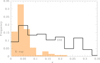
Figure 1. Distribution of cluster redshifts in the ESZ-selected and X-ray-selected samples. The ESZ sample extends to higher redshifts. The solid histogram shows the X-ray flux-limited sample, while the solid line corresponds to the ESZ cluster sample.
Download figure:
Standard image High-resolution image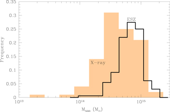
Figure 2. Distribution of cluster masses within r500 for the ESZ-selected and X-ray-selected samples (see Sections 2.1 and 2.2). The X-ray sample extends to lower masses than the ESZ sample. The solid histogram shows the X-ray flux-limited sample, while the solid line corresponds to the ESZ cluster sample.
Download figure:
Standard image High-resolution image2.4. Subclusters
A small fraction (∼10%–20%) of the clusters in both the X-ray and SZ samples present X-ray-bright subclusters. In our analyses we exclude the secondary subclusters. Only the principal cluster component is used in the comparisons between the X-ray and SZ samples. However, we present the metrics for all cluster components in Tables 4 and 5.
3. Data Reduction
Our Chandra data reduction followed the process described in Vikhlinin et al. (2005). We applied the calibration files CALDB 4.7.2. The data reduction included corrections for the time dependence of the charge transfer inefficiency and gain, and also a check for periods of high background, which were then omitted. Standard blank sky background files and readout artifacts were subtracted. We also detected compact X-ray sources in the 0.7–2.0 keV and 2.0–7.0 keV bands using CIAO wavdetect and then masked these sources before performing the spectral and spatial analyses of the cluster emission. For each cluster, we used all available Chandra observations within 2 Mpc of the cluster center with all CCDs (ACIS-I and ACIS-S).
4. Emission Measure Profiles
We refer to Vikhlinin et al. (2006) for a detailed description of the procedures we used to compute the emission measure profile for each cluster. We outline here only the main aspects of the method.
We measured the surface brightness profiles in the 0.7–2.0 keV energy band, which maximizes the signal-to-noise ratio in Chandra observations for typical cluster gas temperatures. We used the X-ray halo peak as the cluster center. The readout artifacts and blank-field background (see Section 2.3.3 of Vikhlinin et al. 2006) were subtracted from the X-ray images, and the results were then exposure-corrected, using exposure maps computed assuming an absorbed optically thin thermal plasma with kT = 5.0 keV, abundance = 0.3 solar, with the Galactic column density and including corrections for bad pixels and CCD gaps, which do not take into account spatial variations of the effective area. We subtracted any small uniform component corresponding to soft X-ray foreground adjustments, if required (determined by fitting a thermal model in a region of the detector field distant from the cluster center, taking into account the expected thermal contribution from the cluster).
Following these steps, we extracted the surface brightness in narrow concentric annuli ( ) centered on the X-ray halo peak and computed the Chandra area-averaged effective area for each annulus (see Vikhlinin et al. (2005), for details on calculating the effective area). To compute the emission measure and temperature profiles, we assumed spherical symmetry. The spherical assumption is expected to introduce only small deviations in the emission measure profile (Piffaretti et al. 2003). Using the modeled deprojected temperature (see Section 7), effective area, and metallicity as a function of radius, we converted the Chandra count rate in the 0.7–2.0 keV band into the emission integral,
  , within each cylindrical shell. Tables 4 and 5 list the maximum cluster radius where the emission integral is computed (
 ) for each cluster. Seven clusters in the ESZ sample have
  , and in the X-ray sample, nine clusters have this condition (four of them are also in the ESZ sample). These numbers represent only 4% and 9% of the clusters in the ESZ and X-ray samples, respectively.
We fit the emission measure profile assuming the gas density profile follows that given by Vikhlinin et al. (2006):
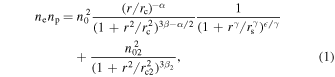
where the parameters n0 and n02 determine the normalizations of both additive components.  , and
, and are indexes controlling the slope of the curve at characteristic radii given by the parameters
 ,
,  , and
, and  . γ controls the width of the transition region given by
  . Although the relation given by Equation (1) is based on a classic β-model (Cavaliere & Fusco-Femiano 1976), it is modified to account for a central power-law type cusp and a steeper emission measure slope at large radii. In addition, a second β-model is included, to better characterize the cluster core. For further details on this equation, we refer the reader to Vikhlinin et al. (2006). In the fit to the emissivity profile, all parameters are free to vary. For a typical metallicity of 0.3
  , the reference values from Anders & Grevesse (1989) yield
  . Examples of projected emissivity and gas density profiles are presented in Figures 3 and 4.
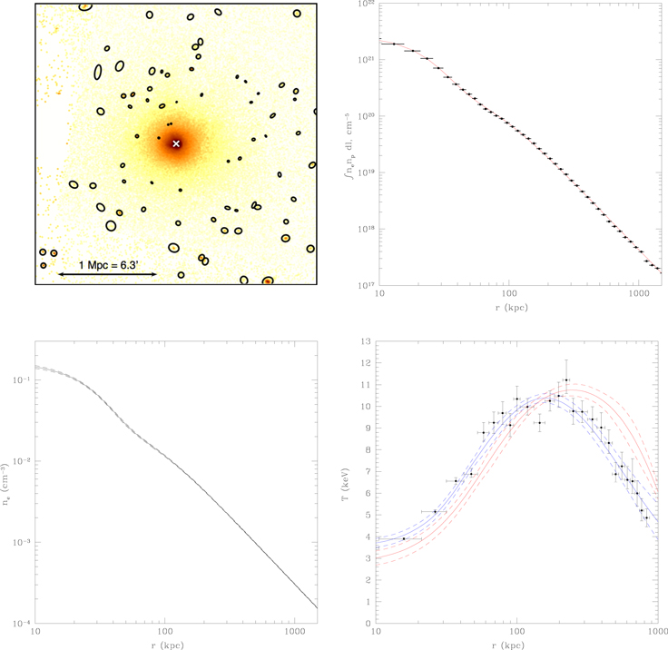
Figure 3. Example of the X-ray image and the projected emissivity, gas density, and temperature profiles for a CC cluster (A2204). The top left panel shows the 0.5–2.0 keV, background-subtracted, exposure-map-corrected ACIS-I image. The total filtered Chandra exposure is 117 ks. The black ellipses correspond to the masked X-ray point sources and the cross corresponds to the cluster center. The top right panel shows the projected emissivity profile. The solid line shows the emission measure integral of the best fit to the emissivity profile given by Equation (1). The bottom left panel shows the gas density profile. The solid line shows the density profile obtained from the emissivity profile given by Equation (1). The bottom right panel shows the gas temperature profile. The red and blue lines show the deprojected and projected temperature profiles, respectively (Equations (7) and 8). The dashed lines in the gas and temperature profiles show the 68% confidence range. This is an example of a cluster with deep Chandra exposure, which allow us to extract the temperature profile in many radial bins.
Download figure:
Standard image High-resolution image5. Total Cluster Mass Estimates
Using the gas mass and temperature, we estimated the total cluster mass from the YX–M scaling relation of Vikhlinin et al. (2009a),

where  is computed using the best-fit parameters of Equation (1), and
  is the measured temperature in the (0.15–1)
  range.
  and
and  (Maughan et al. 2012). Here,
  is the total mass within r500, and
 ![$E(z)\,={{[{{\rm{\Omega }}}_{{\rm{M}}}{(1+z)}^{3}+(1-{{\rm{\Omega }}}_{{\rm{M}}}-{{\rm{\Omega }}}_{{\rm{\Lambda }}})(1+z)}^{2}+{{\rm{\Omega }}}_{{\rm{\Lambda }}}]}^{1/2}$](https://content.cld.iop.org/journals/0004-637X/843/1/76/revision1/apjaa7461ieqn33.gif) is the function describing the evolution of the Hubble parameter.
is the function describing the evolution of the Hubble parameter.
Using Equation (2), r500 is computed by solving

where  is the critical density of the universe at the cluster redshift. In practice, Equation (2) is evaluated at a given radius, whose result is compared to the evaluation of Equation (3) at the same radius. This process is repeated in an iterative procedure, until the fractional mass difference is less than 1%.
6. Cool-core Metrics
It is not possible to measure the temperature profile to determine the presence of a cool core for all clusters in our SZ and X-ray samples because of the X-ray data quality. Figures 3 and 4 illustrate the difference in data quality in the sample. Instead, we apply a more robust approach of using four metrics, described below, to characterize the presence of cool cores.

Figure 4. Similar panels as in Figure 3, for the non-CC cluster PLCKESZ G000.44-41.83. This is an example of a cluster with moderate data quality, which illustrates the necessity of metrics to determine the nature of the cluster core in the absence of a detailed temperature profile, like that shown in Figure 3. The total filtered Chandra exposure is 14 ks.
Download figure:
Standard image High-resolution image6.1. Concentration Parameter in the 40–400 kpc Range
The presence of cooler gas in the cores of clusters usually implies a larger gas density in the core, compared to the gas density outside the core, to maintain the pressure balance. This increased gas density produces an X-ray-bright core, since the X-ray emissivity is roughly proportional to the square of the gas density. Evaluating the X-ray brightness in the cluster core compared to the brightness within a given larger radius is a powerful method to determine if the cluster contains a cool core. This metric is referred to as the concentration parameter and was originally introduced by Santos et al. (2008):

where  is the integrated projected emissivity within a circle of radius r.
6.2. Concentration Parameter in the 0.15–1.0 r500 Range
Here we also use a modification of the original definition (Santos et al. 2008), which is scaled by the characteristic radius r500 as (Maughan et al. 2012):

6.3. Cuspiness of the Gas Density Profile
A third related metric is the cuspiness of the gas density profile computed at a fixed scaled radius of  (Vikhlinin et al. 2007):

where n(r) is the gas density at a distance r from the cluster center.
6.4. Central Gas Density
A fourth useful quantity that indicates if a cluster presents a cool core is the central gas density (Hudson et al. 2010). Here we calculate the central density at 0.01 r500 from the core (which will be called  ), since the equation used to fit the density profile may diverge at r = 0 (if
  in Equation (1)).
7. Temperature Profiles
In this paper, we present the temperature profiles for only two clusters, although we have temperature profiles for all clusters in our samples, which vary in the number of fitted parameters according to the quality of the data. We provide the fitted parameters for all clusters in Andrade-Santos et al. (2017). The two temperature profiles presented in this paper are examples of CC and non-CC (NCC) clusters as well as clusters with very different data quality (see Figures 3 and 4). In this section, we present the analytic equations used to obtain the profiles, referring the reader to papers where the full descriptions of the calculations are presented (see Vikhlinin et al. 2006; Andrade-Santos et al. 2015, 2016).
Vikhlinin et al. (2006) give a 3D temperature profile that describes the general features of the temperature profile of clusters:

where  .
.  and
and  are the transition and CC radii, respectively.
  is the central temperature, and
  , and
, and  are indexes that determine the slopes of the temperature profile in different radial ranges.
We derive the deprojected 3D temperature by projecting a model to compare to the projected measured temperature. The 3D temperature model, T3D, is weighted by the density squared according to the spectroscopic-like temperature (Mazzotta et al. 2004 presented a formula to project the temperature that matches the spectroscopically measured temperature within a few percent):

to give values of T2D for comparison with the measured values.  is the electron density, given by Equation (1), and
  is the deprojected 3D temperature, given by Equation (7).
8. Results
With the cluster gas density and emission measure profiles, we are able to compute the cuspiness of the gas density profile, concentration, and central gas density for the X-ray and Planck ESZ cluster samples. The uncertainties on the metrics for each cluster were computed using 100 Monte Carlo realizations of the density profile, also including a Gaussian distribution for r500 ( ). The top left panel of Figure 5 presents the distribution of concentration parameters in the 0.15–1.0 r500 range for both cluster samples. We used a Kolmogorov–Smirnov (K–S) test for the SZ and X-ray samples to evaluate the probability that the two samples were drawn from the same distribution. We obtained p-values that are smaller than 3.1
  for all metrics, which suggests that the fraction of cool cores in the sample of X-ray-selected clusters is different from that in the SZ sample. Defining a CC cluster as one that presents a concentration parameter in the 0.15–1.0 r500 range,
  , the fraction of cool cores in the X-ray sample is 44% ± 7%, whereas in the SZ sample, the fraction is 28% ± 4%. The uncertainties on the fraction of CC clusters were computed using a Bootstrap re-sampling method, including Poisson statistics on the number of clusters satisfying the CC criterion: a metric value greater than the break value used to segregate clusters into CC and NCC. With a break value of 0.075 (Santos et al. 2008) for the concentration parameter in the 40–400 kpc range (Figure 5, top right panel), we have a CC fraction of 61 ± 8% in the X-ray sample and 36 ± 5% in the SZ sample. The high fraction of CC clusters in the X-ray selected sample compared to that in the SZ sample agrees quite well with the recent results presented by Rossetti et al. (2017) (59% ± 5% in their X-ray sample versus 29% ± 4% in their SZ sample). With a break value of 0.5 (Vikhlinin et al. 2007) for the cuspiness of the gas density profile (Figure 5, bottom left panel), we have a CC fraction of 64% ± 8% in the X-ray sample and 38% ± 5% in the SZ sample. Maughan et al. (2012) used a value of 0.8, more appropriate for moderate to strong CC clusters. They also used a break value of 0.5 for the concentration parameter in the 0.15–1.0 r500 range, which we chose to be 0.4 to also include weak CC clusters. Finally, using a break value of
  (Hudson et al. 2010) for the central gas density to distinguish CC and NCC clusters (Figure 5, bottom right panel), we find that 53% ± 7% of the clusters in the X-ray sample have cool cores, whereas the SZ sample shows a fraction of 39% ± 5%. The fractions of CC clusters and K–S test results are listed in Table 1. We also include in Table 1 a systematic uncertainty on the fraction of CC clusters by varying the break value by ±10%. The magnitude of this systematic uncertainty is comparable to the statistical uncertainty.
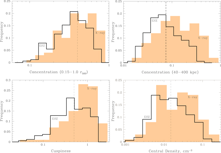
Figure 5. Top left: distribution of the concentration parameter in the 0.15–1.0 r500 range ( —see Equation (5)) for the 164 Planck ESZ-selected (solid line) and the 100 X-ray-selected clusters (orange shaded). Top right: distribution of the concentration parameter in the 40–400 kpc range (
 —see Equation (4)) for both samples. Bottom left: distribution of the cuspiness (δ—see Equation (6)) for both samples. Bottom right: distribution of the central density (
 ) for both samples. The dashed vertical line in each panel corresponds to the break value used to segregate clusters into CC and NCC subsamples (0.4 for the concentration parameter in the 0.15–1.0 r500 range, 0.075 for the concentration parameter in the 40–400 kpc range, 0.5 for the cuspiness, and
  for the central gas density).
Download figure:
Standard image High-resolution imageTable 1. Cool-core Metrics Systematic Uncertainty is Computed by Varying the Break Value by ±10%
| Metric | K–S p-value | Break Value | CC fraction X-ray (%) | CC fraction ESZ (%) |
|---|---|---|---|---|
 : Concentration (0.15–1.0 r500) : Concentration (0.15–1.0 r500) |
3.1 × 10⁻² | 0.4 | 44 ± 7 ( ) ) |
28 ± 4 ( ) ) |
 : Concentration (40–400 kpc) : Concentration (40–400 kpc) |
2.9 × 10⁻⁴ | 0.075 | 61 ± 8 ( ) ) |
36 ± 5 ( ) ) |
| δ: Cuspiness | 1.1 × 10⁻⁴ | 0.5 | 64 ± 8 ( ) ) |
38 ± 5 ( ) ) |
 : Central Density : Central Density |
1.9 × 10⁻² | 1.5 × 10⁻² cm−3 | 53 ± 7 ( ) ) |
39 ± 5 ( ) ) |
Download table as: ASCIITypeset image
Using all four comparisons of the X-ray and SZ cluster samples, we find that CC clusters are significantly more common in X-ray-selected cluster samples than in SZ-selected samples.
Figure 6 shows the correlations between all metrics. Visually, we observe a strong correlation between all metrics, which we verified numerically using a Spearman test. This provides a correlation coefficient ranging between 0 (no correlation) and (−)+1, in the case of perfect (anti)correlation. Results for our metrics are listed in Table 2.
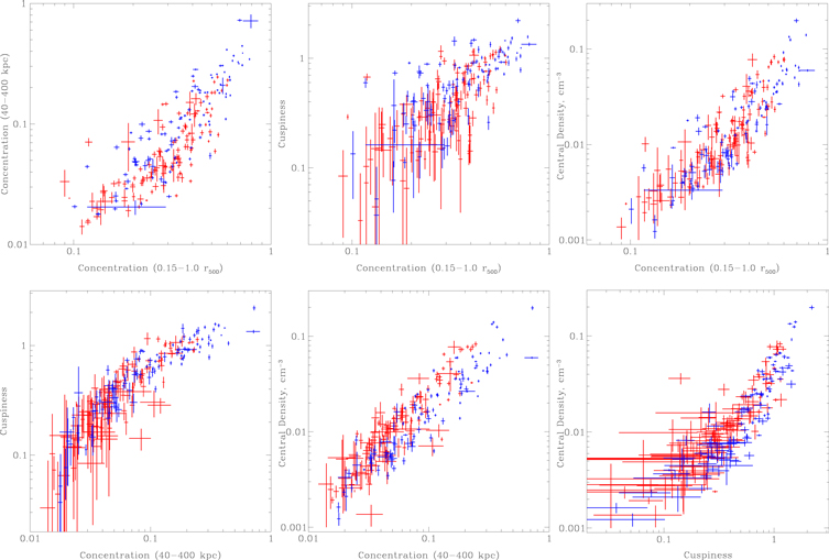
Figure 6. Top left: concentration parameter in the 40–400 kpc range ( ) vs. concentration parameter in the 0.15–1.0 r500 range (
 ). Top center: cuspiness (δ) vs. concentration parameter in the 0.15–1.0 r500 range (
 ). Top right: central density (
 ) vs. concentration parameter in the 0.15–1.0 r500 range (
 ) . Bottom left: cuspiness (δ) vs. concentration parameter in the 40–400 kpc range (
 ). Bottom center: central density (
 ) vs. concentration parameter in the 40–400 kpc range (
 ). Bottom right: central density (
 ) vs. cuspiness (δ). The ESZ sample is in red and the X-ray sample is in blue. This figure shows the strong correlation between different metrics, whose correlations are quantified in Table 2.
Download figure:
Standard image High-resolution imageTable 2. Spearman Rank Test
| Relation | Correlation (X-Ray) | Correlation (ESZ) |
|---|---|---|
 versus versus 
|
0.87 | 0.84 |
 versus δ versus δ |
0.75 | 0.69 |
 versus versus 
|
0.90 | 0.87 |
 versus δ versus δ |
0.93 | 0.90 |
 versus versus 
|
0.93 | 0.91 |
δ versus 
|
0.92 | 0.88 |
Download table as: ASCIITypeset image
Using a set of cosmological hydrodynamic simulations of galaxy clusters, Rasia et al. (2015) found that 38% (11/29) of their simulated clusters at z = 0 are classified as CC using the central entropy (Cavagnolo et al. 2009) and pseudo-entropy ratio (Leccardi et al. 2010) as metrics. This result agrees very well with our observed fraction of CC clusters in the SZ sample (28%–39% according to the metric used, suggesting that the fraction of CC clusters in SZ samples is representative of the fraction of CC clusters in the universe). Lin et al. (2015) showed that constraints on the fraction of CC clusters in SZ-selected data sets are only subject to a systematic bias of the order of one percent, a significant reduction compared to X-ray-selected samples, supporting that SZ-selected samples of galaxy clusters are robust cosmological probes.
8.1. Numerical Simulations
In this section, we apply the four metrics used in this paper to the set of numerical simulations of galaxy clusters from Rasia et al. (2015). We obtain the following results: (a) using the concentration parameter in the 0.15–1.0 r500 range, we obtain a fraction of CC clusters of 33% ± 11%, (b) using the concentration parameter in the 40–400 kpc range, the fraction of CC clusters is 26% ± 10%, (c) using the cuspiness of the gas density, the fraction of CC clusters is 38% ± 11%, and (d) using the central gas density, the fraction of CC clusters is 48% ± 13%. These numbers are in good agreement with the fraction of CC clusters in our ESZ sample.
9. Selection Effects: Malmquist Bias in X-Rays
The X-ray cluster sample used in this paper is derived from the ROSAT X-ray catalogs, which formally used the total X-ray flux as the only selection criterion. Thus, it can be affected by the Malmquist bias, leading to overrepresentation of the CC clusters. CC clusters tend to be more X-ray-luminous for the same mass and thus they become overrepresented in a purely X-ray, flux-limited survey. To estimate the fractional increase in the X-ray luminosity of the CC subsample, we compare the ratio of the observed luminosity to the expected luminosity for the measured mass (using the  –M relation given by Equation (22) from Vikhlinin et al. 2009a) for CC and NCC clusters for all four metrics used to identify CC clusters. We find that CC clusters are on average ∼1.6–1.8 times more X-ray-luminous for the same mass (Table 3) than are NCC clusters. These results are consistent with early studies based on Einstein imaging data (central excesses over the β-model, Jones & Forman 1999), and normalizations of the
  —T relations for the CC and NCC populations (Allen & Fabian 1998).
Table 3. Overpopulation of CC Clusters
| Metric |

|
Expected Overpopulation | Observed Overpopulation |
|---|---|---|---|

|
1.80 ± 0.16 | 2.7 ± 1.0 | 1.6 ± 0.3 |

|
1.63 ± 0.15 | 2.3 ± 0.7 | 1.7 ± 0.3 |
| δ | 1.57 ± 0.15 | 2.1 ± 0.7 | 1.7 ± 0.3 |

|
1.69 ± 0.15 | 2.4 ± 0.8 | 1.4 ± 0.3 |
Download table as: ASCIITypeset image
The impact of this difference in the total X-ray luminosity on the fractions of CC and NCC clusters is substantial. In a low-z flux-limited survey, the search volume is  so a subpopulation that is intrinsically more luminous by a factor of ∼1.7 becomes overrepresented by a factor of 2.2 above a fixed mass threshold.
A similar bias is still present if we consider clusters in a narrow redshift range, where there is no difference in the search volume. In this case, a flux limit is equivalent to an X-ray luminosity threshold. CC clusters are less massive than NCC clusters for a fixed  and hence are more numerous than NCC clusters.
We can quantify the selection effects of CC clusters in X-ray surveys. For simplicity, let us approximate the cluster mass function locally as a power law given by:

and assume a power law M– relation as:

Let l be the ratio of average luminosities (0.5–2.0 keV band, in the  range) at a fixed mass for the CC and NCC populations:

then we would expect the ratio of the number of CC to NCC clusters to be:

We computed the ratio of average luminosities at a fixed mass for the CC and NCC populations, l, to be in the range 1.6–1.8 (Table 3). From Vikhlinin et al. (2009a),  . To compute the slope of the halo mass function, we averaged the slope of the mass function at the location of each cluster mass in our X-ray sample, using the mass function provided by Warren et al. (2006). We obtained
  . With these numbers in hand, we estimate that the CC clusters are overrepresented in our X-ray sample by a factor of Δ = 2.1–2.7 (depending on the metric) because of the Malmquist bias.
10. Conclusions
Using Chandra observations, we derived and compared the fraction of CC clusters in the Planck Early Sunyaev–Zel’dovich (ESZ) sample of 164 detected clusters with  and in a flux-limited X-ray sample of 100 clusters with
  . We use four metrics to identify the presence of a cool core: (1) the concentration parameter, which is the ratio of the integrated surface brightness within 0.15 r500 to that within r500; (2) within 40 kpc to that within 400 kpc; (3) the cuspiness of the gas density profile, which is the negative of the logarithmic derivative of the gas density with respect to the radius measured at 0.04 r500; and (4) the central gas density, measured at 0.01 r500. We list our findings.
- 1.In all four metrics that we used, the sample of X-ray-selected clusters contains a significantly larger fraction of CC clusters compared to the sample of SZ-selected clusters (44% ± 7% versus 28% ± 4% using the concentration parameter in the 0.15–1.0 r500 range as a metric for cool cores, 61% ± 8% versus 36% ± 5% using the concentration parameter in the 40–400 kpc range, 64% ± 8% versus 38% ± 5% using the cuspiness, and 53% ± 7% versus 39% ± 5% using the central density). Our results for the concentration parameter in the 40–400 kpc range agree well with the recent results by Rossetti et al. (2017).
- 2.Qualitatively, CC clusters are more X-ray-luminous at fixed mass. Hence, our X-ray flux-limited sample, compared to the approximately mass-limited SZ sample, is overrepresented with CC clusters. We describe a simple quantitative model that successfully predicts the observed difference based on the selection bias. Our model predicts an overpopulation of CC clusters in our X-ray-selected sample compared to SZ samples of 2.1–2.7, depending on the metric used to identify CC clusters, with a typical uncertainty of ∼0.8, which is consistent within the uncertainties with the observed values in the range 1.4–1.7, with a typical uncertainty of ∼0.3.
- 3.The results of the four metrics we used to measure the overpopulation of CC clusters in X-ray samples, compared to the results for SZ samples, are all consistent within their uncertainties.
- 4.While differences in X-ray and SZ cluster selection are significant, they can be quantitatively explained by the effect of cool cores on X-ray luminosities.
CC clusters are more X-ray luminous than NCC clusters for a fixed cluster mass. Thus, an X-ray flux-limited sample will select a larger fraction of CC clusters compared to an SZ-selected cluster sample. The determination of cosmological parameters from an X-ray flux-limited sample in the local universe can be summarized by determining confidence levels in the highly degenerate  –
– plane. If cluster masses are determined using a proxy other than the X-ray luminosity (e.g., gas mass, M–
 scaling relation,
  , weak-lensing, hydrostatic mass) there will be no Malmquist bias on the determination of cosmological parameters, simply because when the mass function is constructed, the CC clusters that were wrongly included in the selection will now be excluded from the mass function because they do not satisfy the criterion that their masses are above the mass limit given their redshifts. On the other hand, if the cluster masses are determined by the
  –M scaling relation, the masses of the CC clusters will be biased high, and their inclusion in the mass function will lead to a shift toward higher values of
  and
and  .
.
F.A.S. acknowledges support from Chandra grant GO3-14131X. C.J., W.R.F., and A.V. are supported by the Smithsonian Institution. R.J.W. is supported by a Clay Fellowship awarded by the Harvard-Smithsonian Center for Astrophysics. Basic research in radio astronomy at the Naval Research Laboratory by S.G. and T.E.C. is supported by 6.1 base funding. S.B. acknowledges financial support from the PRIN-MIUR 201278X4FL grant. M.A., G.W.P., and J.D. acknowledge support from the European Research Council under the European Union’s Seventh Framework Programme (FP7/2007-2013)/ERC grant agreement n° 340519. L.L. acknowledges support from the Chandra X-ray Observatory grant GO3-14130B and by the Chandra X-ray Center through NASA contract NAS8-03060. We thank the anonymous referee for the useful comments.
Appendix
We present in Table 4 the values of the metrics for all clusters in the ESZ sample, including the secondary subclusters (on the lines following the primary subcluster, indicated by –). Columns list the cluster name (the prefix PLCKESZ is omitted for simplicity), R.A., decl., redshift, concentration parameter in the 0.15–1.0 r500 range, concentration parameter in the 40–400 kpc range, cuspiness of the gas density profile, central gas density, and the maximum radius where the emission integral is computed. Each metric value is followed by its uncertainty.
Table 4. Concentration Parameter, Cuspiness, and Central Density for the Planck ESZ Sample
| Cluster | R.A. | Decl. | z |

|

|

|

|
δ |

|

|

|

|
|---|---|---|---|---|---|---|---|---|---|---|---|---|
| (cm−3) | (cm−3) | (r500) | ||||||||||
| G000.44-41.83 | 21:04:18.603 | −41:20:39.36 | 0.165 | 0.275 | 0.008 | 0.0585 | 0.0044 | 0.611 | 0.084 | 0.01482 | 0.00233 | 1.68 |
| G002.74-56.18 | 22:18:39.822 | −38:53:58.47 | 0.141 | 0.393 | 0.007 | 0.0604 | 0.0030 | 0.254 | 0.047 | 0.01423 | 0.00371 | 1.55 |
| G003.90-59.41 | 22:34:27.334 | −37:44:07.88 | 0.151 | 0.391 | 0.007 | 0.0335 | 0.0011 | 0.135 | 0.029 | 0.00729 | 0.00113 | 1.37 |
| G006.47+50.54 | 15:10:56.117 | +5:44:40.38 | 0.077 | 0.591 | 0.005 | 0.1674 | 0.0035 | 0.920 | 0.015 | 0.05946 | 0.00131 | 1.43 |
| G006.70-35.54 | 20:34:46.912 | −35:49:24.54 | 0.089 | 0.188 | 0.006 | 0.0334 | 0.0016 | 0.251 | 0.048 | 0.00469 | 0.00096 | 1.66 |
| G006.78+30.46 | 16:15:46.073 | −6:08:54.61 | 0.203 | 0.304 | 0.009 | 0.0250 | 0.0008 | 0.159 | 0.030 | 0.00819 | 0.00096 | 1.08 |
| G008.30-64.75 | 22:58:48.095 | −34:48:04.62 | 0.312 | 0.218 | 0.005 | 0.0422 | 0.0020 | 0.289 | 0.047 | 0.00831 | 0.00070 | 1.50 |
| G008.44-56.35 | 22:17:45.701 | −35:43:32.55 | 0.149 | 0.370 | 0.009 | 0.0939 | 0.0049 | 0.614 | 0.056 | 0.01607 | 0.00215 | 1.82 |
| G008.93-81.23 | 0:14:19.305 | −30:23:29.33 | 0.307 | 0.249 | 0.004 | 0.0273 | 0.0011 | 0.212 | 0.048 | 0.00813 | 0.00153 | 1.37 |
Only a portion of this table is shown here to demonstrate its form and content. A machine-readable version of the full table is available.
Download table as: DataTypeset image
We present in Table 5 the values of the metrics for all clusters in the X-ray sample, including the secondary subclusters (on the lines following the primary subcluster, indicated by –). Columns list the cluster name, Planck name (the prefix PLCKESZ is omitted for simplicity; † the prefix PSZ1 is omitted for simplicity), R.A., decl., redshift, concentration parameter in the 0.15–1.0 r500 range, concentration parameter in the 40–400 kpc range, cuspiness of the gas density profile, central gas density, and the maximum radius where the emission integral is computed. Each metric value is followed by its uncertainty.
Table 5. Concentration Parameter, Cuspiness, and Central Density for the X-Ray Sample
| Cluster | Planck Name | R.A. | Decl. | z |

|

|

|

|
δ |

|

|

|

|
|---|---|---|---|---|---|---|---|---|---|---|---|---|---|
| (cm−3) | (cm−3) | (r500) | |||||||||||
| 2A0335 | G176.28-35.05 | 03:38:40.698 | +09:58:03.07 | 0.035 | 0.718 | 0.004 | 0.3876 | 0.0047 | 1.242 | 0.017 | 0.05916 | 0.00104 | 1.09 |
| A85 | G115.16-72.09 | 00:41:50.390 | −09:18:09.53 | 0.056 | 0.455 | 0.004 | 0.1535 | 0.0030 | 1.012 | 0.040 | 0.04534 | 0.00113 | 1.40 |
| A119 | G125.58-64.14 | 00:56:16.210 | −01:14:58.98 | 0.044 | 0.164 | 0.004 | 0.0229 | 0.0007 | 0.221 | 0.052 | 0.00258 | 0.00027 | 1.58 |
| A133 | G149.55-84.16† | 01:02:41.707 | −21:52:52.58 | 0.057 | 0.503 | 0.005 | 0.2421 | 0.0045 | 1.335 | 0.077 | 0.04650 | 0.00115 | 1.98 |
| A193 | 01:25:07.559 | +08:41:59.95 | 0.049 | 0.295 | 0.006 | 0.0596 | 0.0016 | 0.428 | 0.036 | 0.00825 | 0.00085 | 1.44 | |
| A376 | 02:46:03.910 | +36:54:18.44 | 0.049 | 0.240 | 0.008 | 0.0870 | 0.0031 | 0.884 | 0.026 | 0.01538 | 0.00068 | 1.94 | |
| A399 | 02:57:53.422 | +13:01:57.47 | 0.071 | 0.251 | 0.004 | 0.0357 | 0.0012 | 0.339 | 0.049 | 0.00643 | 0.00086 | 1.52 | |
| A401 | G164.18-38.89 | 02:58:57.595 | +13:34:44.19 | 0.074 | 0.308 | 0.005 | 0.0400 | 0.0012 | 0.262 | 0.040 | 0.00776 | 0.00081 | 1.34 |
| A478 | G182.44-28.29 | 04:13:25.196 | +10:27:53.66 | 0.088 | 0.622 | 0.005 | 0.1726 | 0.0033 | 0.908 | 0.056 | 0.05973 | 0.00179 | 1.38 |
| A496 | G209.56-36.49 | 04:33:37.913 | −13:15:42.03 | 0.033 | 0.438 | 0.005 | 0.1892 | 0.0039 | 1.200 | 0.086 | 0.04229 | 0.00359 | 0.79 |
Only a portion of this table is shown here to demonstrate its form and content. A machine-readable version of the full table is available.
Download table as: DataTypeset image