Abstract
In this paper, we employ a path-conservative HLLEM finite-volume method (FVM) to solve the solar wind magnetohydrodynamics (MHD) systems of extended generalized Lagrange multiplier (EGLM) formulation with Galilean invariance (G-EGLM MHD equations). The governing equations of single-fluid solar wind plasma MHD are advanced by using a one-step MUSCL-type time integration with the logarithmic spacetime reconstruction. The code is programmed in FORTRAN language with Message Passing Interface parallelization in spherical coordinates with a six-component grid system. Then, the large-scale solar coronal structures during Carrington rotations (CRs) 2048, 2069, 2097, and 2121 are simulated by inputting the line-of-sight magnetic field provided by the Global Oscillation Network Group (GONG). These four CRs belong to the declining, minimum, rising, and maximum phases of solar activity. Numerical results basically generate the observed characteristics of structured solar wind and thus show the code’s capability of simulating solar corona with complex magnetic topology.
1. Introduction
The ambient solar wind is the unique channel through which solar eruptions like coronal mass ejections (CMEs) evolve and propagate, and along which energetic particles are transported. Therefore, the ambient solar wind study is of importance. 3D magnetohydrodynamics (MHD) solar wind models (e.g., Mikić et al. 1999; Feng et al. 2011a, 2013; Lionello et al. 2013; van der Holst et al. 2014; Wu & Dryer 2015) are effective tools for us to physically understand solar wind, since the MHD modeling is currently the only self-consistent method capable of bridging the large heliocentric distances from near the Sun to well beyond Earth’s orbit. Along with this line, various MHD models have been developed (e.g., Roussev et al. 2003; Usmanov & Goldstein 2003; Cohen et al. 2007; Nakamizo et al. 2009; Feng et al. 2010, 2011b, 2012b, 2014a, 2014b, 2015; Riley et al. 2012; Tóth et al. 2012). For a survey, refer to Wu & Dryer (2015). Among them, finite-volume methods (FVMs) based on approximate Riemann solvers are widely used.
In this paper, we are devoted to a new application of the path-conservative HLLEM Riemann solver to the study of solar wind, by advancing the equations of single-fluid solar wind plasma MHD with the one-step MUSCL-type time integration method and the logarithmic spacetime reconstruction. In the following, the HLL family tree is briefly reviewed. Since the birth of the so-called Harten–Lax–van Leer (HLL) approximate Riemann solver proposed by Harten (1983), many HLL-type solvers have been applied with different degrees of success for the MHD equations. Zachary et al. (1994) presented a higher-order Godunov HLL method for 2D and 3D MHD. Motivated by the work of Powell et al. (1999), by allowing magnetic monopoles in MHD equations and properly taking into account the magnetostatic contribution to the Lorentz force, Janhunen (2000) has constructed a positive and conservative HLL scheme hybridized with the Roe solver for ideal MHD. The HLL scheme has also been used (Ziegler 2011; Feng et al. 2014b) on orthogonal-curvilinear grids within a finite-volume framework for the MHD equations. Linde (2002) proposed a general-purpose Riemann solver with two states by including the information of contact discontinuity, where the jump of the intermediate states is empirically connected with the jump of the left and right states. Being independent of the governing equations’ details, Linde’s modified HLLE solver (Harten 1983; Einfeldt 1988; Einfeldt et al. 1991) can be applied for general hyperbolic conservation laws, particularly for the MHD equations. By including additional contact waves, Gurski (2004) presented an HLLC (Harten–Lax–van Leer contact wave) approximate nonlinear Riemann solver for ideal MHD equations, which resolves slow, Alfvén, and contact waves better than the original HLL solver. Motivated by the work of Gurski (2004), Li (2005) presented another variant of the HLLC-type solver for the MHD. In the method of Li (2005), the intermediate states are consistent with the integral of the conservation laws over the Riemann fan, and the solver naturally returns to the HLLC solver for zero magnetic field. Balsara (2012a) presented a genuinely 2D HLLC Riemann solver on logically rectangular meshes, which achieves its stabilization by introducing a constant state in the region of strong interaction and turns the 2D HLL Riemann solver into a 2D HLLC Riemann solver. For unstructured meshes, Balsara et al. (2014) applied the genuinely multidimensional HLLC Riemann solver to compressible gasdynamics and MHD equations to show the twin advantages of isotropic propagation of flow features and a larger CFL number. Guo (2015) presented an extended HLLC Riemann solver for the MHD system with the magnetic field decomposed into a strong internal magnetic field and an external component, which recovers the previously developed HLLC Riemann solver as long as the internal field is set to zero. Considering five waves, researchers constructed the so-called HLL-Discontinuities (HLLD) approximate Riemann solver (e.g., Miyoshi & Kusano 2005; Mignone 2007; Mignone et al. 2009, 2012; Miyoshi et al. 2010; Guo et al. 2016), which is believed to accurately resolve rotational and isolated contact discontinuities in MHD. While HLLC/HLLD Riemann solvers seek to restore an isolated contact discontinuity in the HLL Riemann solver, there are also other ways to introduce intermediate waves such as HLLE and HLLEM Riemann solvers. The 1D HLLE Riemann solver (Einfeldt 1988; Einfeldt et al. 1991) tried to do that by introducing a linear profile in the Riemann fan. Balsara (2010) presented a multidimensional version of the HLLE Riemann solver, which has been accomplished via a simple constructive strategy by introducing one constant resolved state between the states under consideration. Furthermore, the HLLEM solver consists of the HLLE flux plus some anti-diffusion terms to improve the resolution of the waves between the two fastest waves (e.g., Dedner et al. 2001, 2002, 2003, 2005; Wesenberg 2002, 2003; Balsara & Kim 2016; Dumbser & Balsara 2016). Dumbser & Balsara (2016), Balsara (2016), and Balsara & Nkonga (2017) introduced an HLLI Riemann solver (a new formulation of the HLLEM method) to accommodate multiple intermediate waves, with “I” standing for the intermediate characteristic fields that can be accounted for.
The HLL family of Riemann solvers, such as HLL/HLLC/HLLD/HLLE/HLLEM/HLLI types, are robust and efficient. One typical property of these solvers is that they can guarantee the positivity of the density and pressure, at least, for 1D problems. Moreover, their simplicity has gained them considerable popularity. In numerical solar wind simulation, HLL-type solvers have also been employed. For example, Shiota and his coauthors (Shiota et al. 2008, 2010, 2014; Shiota & Kataoka 2016) developed a new MHD model with the GLM form (Dedner et al. 2002) of the background solar wind in the inner heliosphere based on the time series of daily synoptic observations of the photospheric magnetic field (called the SUSANOO-SW model), using an FVM with the HLLD nonlinear Riemann solver (Miyoshi & Kusano 2005; Mignone 2007; Miyoshi et al. 2010). Motivated by the work of Ziegler (2011), Feng et al. (2014b) introduced a new 3D MHD numerical model to simulate the steady-state ambient solar wind from the solar surface to Earth or beyond, with various divergence cleaning approaches (Zhang & Feng 2016). Also, Feng et al. (2011b) proposed a 3D MHD model for solar wind study with hybrid solvers, where the spacetime conservation element and solution element method is used in the near-Sun domain and the HLL method is employed in the off-Sun domain. Janhunen et al. (2012) proposed a global magnetosphere–ionosphere coupling simulation that integrates a 3D MHD simulation of the magnetosphere with a high-resolution ionospheric model. With the HLLD approximate Riemann solver, Miyoshi et al. (2010) developed an MHD algorithm for global simulations of planetary magnetospheres and displayed an example of the solar wind–magnetosphere interaction using the first-order HLLD Riemann solver on a cubed-sphere grid system (Ronchi et al. 1996). Guo (2015) applied the HLLC Riemann solver exemplarily for the interaction between solar wind and the magnetosphere.
Approximate Riemann solvers have been generalized to efficiently handle nonconservative hyperbolic systems with path-conservative methods (Toumi 1992; Maso et al. 1995). In a conservative case, this family of path-conservative schemes can recover well-known Riemann solvers such as the Roe, HLL, HLLC, and Osher-Solomon ones (e.g., Tian et al. 2011; Castro et al. 2014; Nguyen & Dumbser 2015; Dumbser & Balsara 2016; Leibinger et al. 2016; Sánchez-Linares et al. 2016; Feng et al. 2017). Based on the utility of similarity variables (Balsara 2010, 2012a; Balsara et al. 2014; Balsara & Dumbser 2015), for the first time Dumbser & Balsara (2016) presented a path-conservative formulation of the HLLEM Riemann solver for shallow water-type equations and ideal GLM-MHD equations (Dedner et al. 2002).
The purpose of this paper is to implement the path-conservative formulation of the HLLEM Riemann solver in spherical coordinates for the G-EGLM MHD equations and apply it to the numerical study of the global solar corona. To this end, the present paper is organized as follows. In Section 2, the governing MHD equations for the solar wind plasma and magnetic field are specified. Section 3 introduces the grid system and the initial setup, together with the boundary conditions. Section 4 is devoted to the formulation of the path-conservative HLLEM method in spherical coordinates by following Dumbser & Balsara (2016). In Section 5, simulation results are presented. Section 6 summarizes some concluding remarks and discussions. In Appendix A, the modified MHD eigensystem used in the present paper is provided.
2. The Governing Equations of Solar Wind Plasma and Magnetic Field
Currently, and in the foreseeable future, MHD models are the only models that can span the enormous distances presented in the corona interplanetary space, although even generalized MHD equations are only a relatively low-order approximation to more complete physics by providing only a simplified description of natural phenomena in space plasmas. Generally, the ideal MHD equations include the continuity, the momentum, the energy, and the magnetic induction equations, and there are no magnetic sources in a magnetic field, implying that a magnetic field has to satisfy the divergence constraint: ∇ · B = 0. In multidimensional MHD simulations, it is difficult to satisfy the divergence-free constraint (e.g., Powell et al. 1999; Tóth 2000; Dedner et al. 2002; Yee & Sjögreen 2006; Mignone & Tzeferacos 2010; Yalim et al. 2011; Ziegler 2011; Feng et al. 2014a, 2014b; Zhang & Feng 2016). The violation of the divergence constraint is due to the nonphysical intermediate state within a numerical discontinuity profile. Since this violation may frequently lead to severe stability problems, researchers have tried to enforce the divergence-free constraint in their MHD formulations such as the projection method (e.g., Brackbill & Barnes 1980; Tanaka 1994; Zachary et al. 1994; Tóth 2000; Serna 2009), constraint transport method (e.g., Yee 1966; Evans & Hawley 1988; Ziegler 2011; Feng et al. 2014b; Christlieb et al. 2015; Zhang & Feng 2016), eight-wave solution method (e.g., Powell et al. 1999; Jones et al. 1997; Tóth 2000; Fuchs et al. 2010; Ivan et al. 2013), and hyperbolic divergence cleaning method (e.g., Dedner et al. 2002; Han et al. 2009; Yalim et al. 2011; Jiang et al. 2012b; Mignone et al. 2012; Susanto et al. 2013).
In the present study, the mixed-type hyperbolic divergence cleaning method by Dedner et al. (2002) is chosen to eliminate divergence errors because it can be easily implemented in a finite-volume numerical scheme without any modification. If we employ the G-EGLM MHD equations (Dedner et al. 2002), then the governing equations for the solar wind plasma and magnetic field read

with a factor of  (μ = 4 × 10⁻⁷π H/m is the magnetic permeability) absorbed in the definition of magnetic field. The variables are density ρ, velocity vector v = (vr, vθ, vϕ), initial potential magnetic field B0 = (Br0, Bθ0, Bϕ0), perturbed magnetic field B1 = (Br1, Bθ1, Bϕ1) changing with time, total magnetic field B = (Br, Bθ, Bϕ), Lagrange multiplier ψ, the solar mass Ms, the solar angular velocity Ω, the gravitational constant G, the time t, and the vector
  , with r the heliocentric distance. The term
 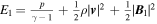 presents the modified total energy density, containing kinetic energy density
  , thermal energy density
  , and the modified magnetic energy density
  .
.  is the thermal pressure, with T the bulk plasma temperature and
  the gas constant (1.653 × 10⁴ m2 s−2 K−1), and γ is the polytropic index, varying from 1.05 to 1.5 along the heliocentric distance r according to Feng et al. (2010, 2014b). ch and cp are the advection speed and the amount of diffusion component in ψ, respectively (Susanto et al. 2013). Without affecting the time step of the numerical simulation process, many authors usually set ch as the largest eigenvalue in the whole computational domain, and then the divergence errors can be convected out of the boundary quickly. Once the coefficient ch is confirmed, then the remaining problem is how to determine the coefficient cp. Eventually, we chose
  as Dedner et al. (2002) did. The details about how to choose the parameter cp are presented in the literature (e.g., Dedner et al. 2002; Han et al. 2009; Mignone & Tzeferacos 2010; Mignone et al. 2010; Jiang et al. 2012a, 2012b; Susanto et al. 2013; Xisto et al. 2013; Feng et al. 2017) and references therein.
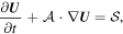
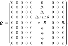
The above G-EGLM form can be seen as the conservative GLM form (Dedner et al. 2002) by adding several source terms written as a product of a matrix Q and a first-order spatial derivative of U. Rewrite Equation (1) in a compact form

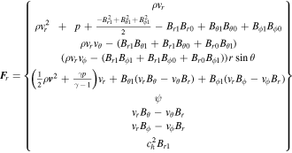
where U = (ρ, ρvr, ρvθ, ρvϕr sin θ, E1, Br1, Bθ1, Bϕ1, ψ) is the state vector of the conserved variables, which, for the typical gasdynamics equations, are related to the conservation of mass, momentum, and energy. The azimuthal component of momentum equation for  in the conservation form is discussed by Feng et al. (2014b). F(U) = [Fr(U), Fθ(U), Fϕ(U)] is the flux tensor for the conservative part of the partial differential equation system, while Q(U) = [Qr(U), Qθ(U), Qϕ(U)] represents the corresponding nonconservative part. Finally, S(U) is the vector of the source terms, consisting of Sflux, SQ, Sgra, Srot, Sheat, and Sψ, that is, S = Sflux + SQ + Sgra + Srot + Sheat + Sψ. The source terms Sflux and SQ are caused by conservative flux and nonconservative products due to the geometrical factors and have the following form:
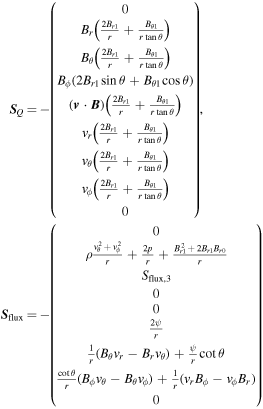
with
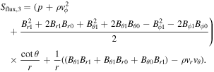
The term Sgra is the external gravitational field. Its concrete form is
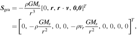
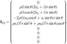
where the gravitational constant  and solar mass Ms = 1.99 × 1030 kg. The term Srot is the rotational effects due to the corotating frame with the Sun. It can be expressed by
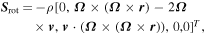
where the solar angular speed  . Specifically,
The term 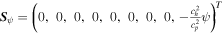 comes from the GLM formulation of Dedner et al. (2002), while
  represents the coronal heating and solar wind acceleration terms. In our case, SM is the momentum source term and SE = QE + vrSM is the energy source term, with QE being the volumetric heating function. The source terms SM and QE are given as follows:
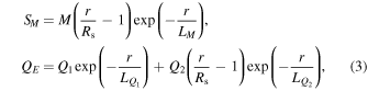
where 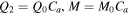 ,
,  , with

Here, fs and θb are the expansion factor of the magnetic field obtained from the PFSS model and the minimum angular separation from the open magnetic field footpoint of the force line through the computed point to the nearest coronal hole (CH) boundary at the photosphere, respectively. The coefficients M0, Q0, Q1,  ,
,  , and LM in Equation (3) are the same as those in Feng et al. (2017).
For convenience, we recast the system (2) in quasi-linear form
where ![${ \mathcal A }({\boldsymbol{U}})=[{{\boldsymbol{A}}}_{r},{{\boldsymbol{A}}}_{\theta },{{\boldsymbol{A}}}_{\phi }]=\tfrac{\partial {\boldsymbol{F}}({\boldsymbol{U}})}{\partial {\boldsymbol{U}}}+{\boldsymbol{Q}}({\boldsymbol{U}})$](https://content.cld.iop.org/journals/0004-637X/867/1/42/revision1/apjaae200ieqn19.gif) accounts for both the conservative and the nonconservative contributions, and the source term
accounts for both the conservative and the nonconservative contributions, and the source term  is slightly different from S in Equation (2) owing to the spherical geometrical factors. For example, the spatial derivative terms in the r-direction take the form

and flux Fr and matrix Qr in the r-direction are
Let the matrix 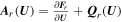 (say, in the radial direction) be the sum of the Jacobian matrix of the flux
  and the genuinely nonconservative part of the system contained in Qr(U). The system’s hyperbolicity means that A(U) has only real eigenvalues with a full set of linearly independent eigenvectors. In the case Q(U) = 0, Equation (1) or Equation (2) reduces to a pure flux form usually called a system of conservation form. Hereafter we will denote the matrix of eigenvalues of Ar(U) with
  , where
  are the eigenvalues of the matrix Ar(U) with the associated left and right eigenvectors denoted by
  ,
,  , and
, and  . Furthermore, assume that the left and right eigenvectors are orthonormal, i.e., Lr Rr = I, where I is the identity matrix. The specific expressions of the eigensystem in the r-direction are listed in Appendix A. Similarly, we can write out Fθ, Fϕ, Qθ, Qϕ, Aθ, Aϕ, and the eigensystems in the θ- and ϕ-directions.
The variables ρ, v, p, r, and t in the above equations are normalized by the characteristic values  ,
,  , where ρs and as are the density and acoustic wave speed at the solar surface of one solar radius Rs, the magnetic fields B, B0, and B1 are characterized by
  , and the solar rotation Ω is normalized by
  . In the end of the computation, these scales are then used to obtain the plasma parameters with dimension for all the variables involved in the system.
3. Grid System and Initial Boundary Value Setup
The grid system we adopt in this paper is the six-component spherical coordinate grid (Feng et al. 2010, 2012a, 2012b, 2012c, 2014a, 2014b), with the coronal model computational region ![$[1{R}_{{\rm{s}}},20{R}_{{\rm{s}}}]\times [0,\pi ]\times [0,2\pi ]$](https://content.cld.iop.org/journals/0004-637X/867/1/42/revision1/apjaae200ieqn32.gif) . That is to say, the spherical shell is divided into six identical components to cover the spherical surface with a partial overlap on their boundaries, and each component is defined identically by low latitudinal region [π/4 − δ1, 3π/4 + δ1] × [3π/4 − δ2, 5π/4 + δ2], with δ1 and δ2 the minimum overlapping grids of two adjacent components in the θ- and ϕ-directions.
. That is to say, the spherical shell is divided into six identical components to cover the spherical surface with a partial overlap on their boundaries, and each component is defined identically by low latitudinal region [π/4 − δ1, 3π/4 + δ1] × [3π/4 − δ2, 5π/4 + δ2], with δ1 and δ2 the minimum overlapping grids of two adjacent components in the θ- and ϕ-directions.
Each basic sliding approximative hexahedron cell (i, j, k) is given by [rim, rip] × [θjm, θjp] × [ϕkm, ϕkp], with spacings Δr(i), Δθ(j), Δϕ(k). The six bounding faces of the control cell are marked by halfway indices im = i − 1/2 (jm = j − 1/2, km = k − 1/2) and ip = i + 1/2 (jp = j + 1/2, kp = k + 1/2), where i = 1, ⋯, Nr, j = 1, …, Nθ, k = 1, ⋯, Nϕ. Starting from  and
and  , the grid mesh is generated by rim = r(i − 1)p, rip = rim + Δr(i), θjm = θ(j−1)p, θjp = θjm + Δθ(j), ϕkm = ϕ(k−1)p, ϕkp = ϕkm + Δϕ(k). The geometrical centers are then denoted by (ri, θj, ϕk) with
 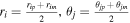 , and
, and  . The volume-averaged coordinates are given by
  with
with  and
and 
 . The coordinates of six face centers are then defined as
  ,
,  ,
,  ,
,  ,
,  , and
, and  , with
  ,
,  , and
, and  .
.
As to the grid partitions, the resolutions in the tangent directions are equally given by Δθ = Δϕ = 15. The grids in the r-direction are highly nonuniform, for 1Rs–20Rs; when
 , the resolution in r-direction is uniform,
  when
when  , then
  with
with  and when
  , then Δr(i) = r(i−1)mΔθ. The overlapping regions of two adjacent components are δ1 = 3Δθ and δ2 = 3Δϕ. Overall, the grid number of our computational region is 127 × 120 × 240.
The initial of the flow field plasma density ρ, radial speed vr, and gas pressure p are obtained through solving Parker’s hydrodynamic isothermal solar wind solution with the initial number density and temperature on the solar surface prescribed to be 1.3 × 10⁶ K and 1.5 × 108 cm3, respectively, and the tangential velocities vθ and vϕ all zeros. The initial 3D global potential magnetic field in the computational domain is obtained through the potential field (PF) model by adopting the line-of-sight photospheric magnetic data from the GONG magnetogram. We interpolate the Global Oscillation Network Group (GONG) Carrington maps, originally in sine latitude format, to a uniform 361 × 181 grid with 1° × 1° cell resolution before the utilization of the PF model. Additionally, given the nature of variable ψ, a good choice for the initial value of the unphysical variable is ψ = 0 (Dedner et al. 2002).
As to the boundaries, we only have inner and outer boundaries for the six-component composite grid system. We adopt the projected normal characteristic (PNC) method (Nakagawa 1980, 1981a, 1981b; Wang et al. 1982, 2011; Nakagawa et al. 1987; Hayashi 2005, 2013; Wu et al. 2006; Feng et al. 2012a) for our inner and outer boundaries. Taking the inner boundary as an example, for the outgoing waves, i.e.,  , the waves propagate out of the computational domain, and then the values at the boundary are defined entirely by the solution at and within the boundary, so the spatial derivative of solution variables in the r-direction may be computed using one-sided difference, and therefore here we adopt the first-order upwind differencing. For the incoming waves, i.e.,
  , the waves propagate from the outside of the computational domain to the inside, and then the values at the boundary depend on the solution exterior to the model volume, and the corresponding spatial derivative of solution variables in the r-direction may be discreted by other methods. Here we adopt the nonreflecting boundary condition, meaning that there is no information entering the computational domain. With the central difference in the transverse θ- and ϕ-directions, we solve the linear equations of time derivatives through the time integration method and obtain the values we needed at the inner boundary cells. In the same manner, we can also complete the update of the variables at our outer boundary cells. Additionally, in the solar corona simulation, only vr > 0 is meaningful since mass flowing away from the Sun is of no interest. If the updated vr from the above bottom boundary condition is negative, that is, vr < 0, then we set ∂p/∂t = 0, ∂ρ/∂t = 0, v = 0, B(t) = B(t), for instance, pn+1(0, θ, ϕ) = pn(0, θ, ϕ) and ρn+1(0, θ, ϕ) = ρn(0, θ, ϕ). If ρn+1 < 0, then ρn+1 = ρn.
4. Path-conservative HLLEM Scheme
For the first time, Dumbser & Balsara (2016) presented a path-conservative formulation of the HLLEM Riemann solver for nonconservative partial differential equations. The proposed scheme naturally inherits the positivity properties and the entropy enforcement of the underlying HLL scheme. In addition, with just the slight additional cost of evaluating eigenvectors and eigenvalues of intermediate characteristic fields, linearly degenerate intermediate waves with a minimum of smearing can be represented. In the following subsections, we present the formulation of the HLLEM scheme for the solar wind MHD systems in spherical coordinates by including the hyperbolic divergence-correction term proposed by Dedner et al. (2002).
4.1. Path-conservative HLLEM Solver
By using a path-conservative HLLEM method (Dumbser & Balsara 2016), the solar wind governing Equations (1) can be written as the following discretized form:
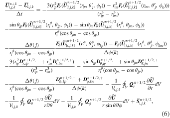
with the jump term D, the flux function F, and the source term S evaluated at the half time level  and cell-averaged variables
  . The integration of the nonconservative product terms can be interpreted by the space reconstruction polynomial and its first-order spatial derivative. For simplicity, this integral can be approached by means of Gaussian quadrature:
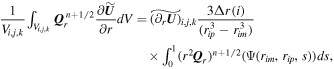
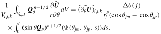
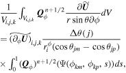
where the terms  ,
,  , and
, and  are defined by
As pointed out by previous works (Feng et al. 2014b, 2017), the integrations of extra source terms in the r- and θ-momentum equations should be treated carefully. To be self-contained, the integrations of any variable  are repeated below:
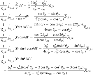
where  is any component function of U.
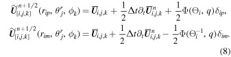
A second-order MUSCL-type scheme in time can then be obtained by the following approximation of the first-order derivative of U in time, which is based on a discretized form of the governing equations as follows:
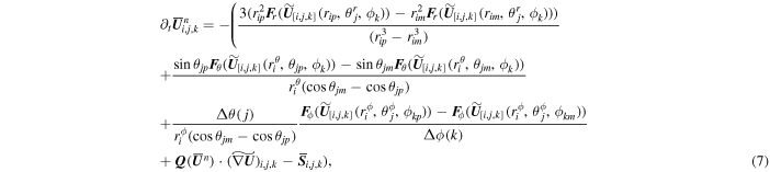
with the gradient 
 . When the reconstructed interface variables, for example,
 ![${\widetilde{{\boldsymbol{U}}}}_{[i,j,k]}({r}_{{ip}},{\theta }_{j}^{r},{\phi }_{k})$](https://content.cld.iop.org/journals/0004-637X/867/1/42/revision1/apjaae200ieqn67.gif) and
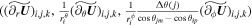
and ![${\widetilde{{\boldsymbol{U}}}}_{[i,j,k]}({r}_{{im}},{\theta }_{j}^{r},{\phi }_{k})$](https://content.cld.iop.org/journals/0004-637X/867/1/42/revision1/apjaae200ieqn68.gif) , are considered, we can use the logarithmic and minmod reconstructions. The logarithmic reconstruction reads (Schmidtmann et al. 2016a, 2016b)
, are considered, we can use the logarithmic and minmod reconstructions. The logarithmic reconstruction reads (Schmidtmann et al. 2016a, 2016b)
where  with
with  ,
,  ,
,  . The choice of the limiter Φ determines the order of accuracy for the reconstruction. Here, we use the following limiter:
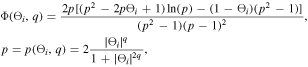
where q = 1.4 is used (Schmidtmann et al. 2016a, 2016b). With the time derivative given in Equation (7), the values at intermediate time levels in Equation (6) can be obtained by the logarithmic spacetime reconstruction:
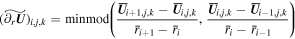
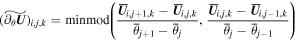
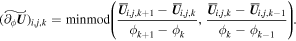
Alternately, the reconstructed interface values in Equation (7) can be achieved by minmod spatial reconstruction (e.g., Ziegler 2011; Feng et al. 2014b, 2017) ![${\widetilde{{\boldsymbol{U}}}}_{[i,j,k]}(r,\theta ,\phi )={\overline{{\boldsymbol{U}}}}_{i,j,k}\,+{(\widetilde{{\partial }_{r}{\boldsymbol{U}}})}_{i,j,k}(r-{\overline{r}}_{i})\,+$](https://content.cld.iop.org/journals/0004-637X/867/1/42/revision1/apjaae200ieqn73.gif)
 . Then the piecewise linear spacetime reconstruction polynomial (e.g., Toro 2009; Nguyen & Dumbser 2015; Leibinger et al. 2016; Feng et al. 2017) can be adopted to calculate the values at intermediate time levels in Equation (6),

For simplicity, we use  , and
, and  to stand for the left state and the right state of the cell interfaces ip and im in the radial direction. Obviously,


The left and right states at the cell interfaces in other directions are defined similarly.
In the following we explain jump terms D in Equation (6) by only pointing out their expressions in the radial direction for the sake of simplicity. The solution strategy for the HLL class of Riemann solvers is to mainly find the constant, resolved HLL state  that lies between the left state
  and the right state
  . The resolved state propagates into the left and right states with speeds sL ≤ 0 and sR ≥ 0. However, entropy enforcement might cause further expansion of the Riemann fan consistent with the physics of the hyperbolic system (see, e.g., Einfeldt 1988; Einfeldt et al. 1991). The speeds sL and sR with the constant intermediate state
  constitute a self-similarly evolving wave model for the 1D HLL Riemann solver. In the HLL method, the entire wave structure of the Riemann problem is only approximated by the two fastest outward-moving waves and one single intermediate state. As usual, we prescribe the following simple wave speed estimates for
  and the right state
  :
:  with the intermediate state
  simply being the arithmetic average
  . With a constant state
  between the left state
  and the right state
  , the HLL fluctuation expression (Ziegler 2011; Feng et al. 2014b; Dumbser & Balsara 2016) reads
for κ ∈ {im, ip}, where  and
and  , commonly denoted by sL and sR in the HLL family, are the left and right wave speed bounds defined just above at
  . Here the intermediate state
  and nonconservative products
  ,
,  will be shown in Appendix B. Since the wave speeds associated with vr ± ch in the G-EGLM MHD system do not transport any physical feature, they are just intended to transport divergence errors out of the computational domain. If the artificial wave speed ch is larger than any physical wave speed, the errors are quickly advected out of the computational domain. For the HLL method to be positive, we must find expressions for the lower and upper bounds sL and sR for the wave speeds of the Riemann problem solution. Being not aware of rigorous bounds for MHD, we can choose the smallest and largest values of vr ± ch. They probably overestimate the true wave speeds somewhat, which may increase the diffusion of the HLL method (Einfeldt et al. 1991). In practice, we can also choose the smallest and largest values of vr ± cf. These choices of wave speed bounds guarantee positivity according to our numerical verification, and the nonexactness of the bounds seems numerically insignificant. We can also use 7 × 7 with the analytical solution Br1, ψ replaced to get rid of this dilemma selection (Dedner et al. 2002; Mignone & Tzeferacos 2010; Mignone et al. 2010; Susanto et al. 2013; Feng et al. 2017).
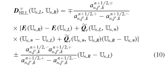
With the definition of DHLL, we are now in a position to state the jump terms involved in the path-conservative HLLEM scheme (Dumbser & Balsara 2016):
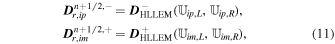
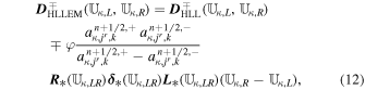
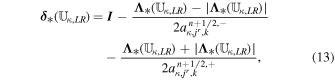
where the first terms on the right-hand side of Equation (12) are defined previously in Equation (10) and the second terms on the right-hand side of Equation (12) are called the anti-diffusive contributions coming from the inclusion of the intermediate waves in the Riemann problem. The derivation and rationality of the diagonal matrix  have been given in Appendix B of Dumbser & Balsara (2016). Here, φ ∈ [0, 1] is a flattener variable (Balsara 2012b; Dumbser & Balsara 2016), which acts to identify regions of strong shocks within the computational domain and plays the role of switching the Riemann solver smoothly from HLL to HLLEM.
4.2. Remarks on HLLEM Solver
As seen from Sections 4.1 and Appendix B, we can treat all nine conservative variables without discrimination and apply the path-conservative HLLEM scheme to the whole numerical flux calculation. This scheme is called “9(HLLEM)” in brief.
Alternatively, if the ninth equation in Equation (1) is decoupled from the full MHD system, we have

The numerical flux of Equation (14) can be separately handled by the Lax–Friedrichs (LF) method (e.g., Chorin 1967; Yalim 2008; Balasubramanian & Anandhanarayanan 2014). For example, this numerical flux Fψ at the interface ip and time tn+1/2 reads as follows:
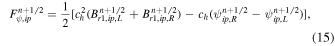
where the subscripts L and R denote the left and right reconstructed states at cell interfaces. The discretized form for Equation (14) becomes
with the numerical fluxes estimated by Equation (15). The source term  is evaluated by the cell-averaged variables at the half time level
  ,
, ![${\overline{S}}_{\psi ,i,j,k}^{n+1/2}=S({\widetilde{{\boldsymbol{U}}}}_{[i,j,k]}^{n+1/2}({\overline{r}}_{i},{\overline{\theta }}_{j},{\phi }_{k}))$](https://content.cld.iop.org/journals/0004-637X/867/1/42/revision1/apjaae200ieqn98.gif) , while the gradient ∇ψ in the source term can be discreted by the Green–Gauss theorem:
, while the gradient ∇ψ in the source term can be discreted by the Green–Gauss theorem:
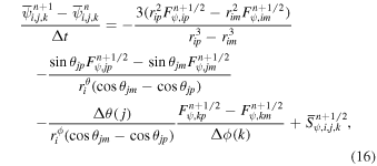
where  denotes the unit outer normal vector of the interface Sl, with l standing for the interface of the control cell (i, j, k). By combining Equation (6) (for the first eight equations) and Equation (16), we obtain the discretized form of the full G-EGLM system. For simplicity, we name this method “8(HLLEM)+1(LF).”
Additionally, in the r-direction, we can decouple the equations  and
and  from the rest of the G-EGLM MHD system (e.g., Dedner et al. 2002; Susanto et al. 2013; Núñez-de la Rosa & Munz 2016) and solve these two equations to obtain the analytical solutions. By substituting the analytical solutions directly into the flux formula
  and
and  , we achieve these two numerical fluxes. Furthermore, the analytical solutions can be used as much as possible to calculate the other seven numerical fluxes when using the HLLEM scheme described above. This scheme is named “7(HLLEM)+2(analytic)” in brief.
5. Numerical Results
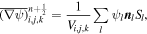
This section displays the numerical results obtained by using the FVM with the “8(HLLEM)+1(LF)” nonlinear Riemann solver introduced in Section 4.2, the logarithmic spacetime reconstruction (8), and the one-step MUSCL-type time integration, with the intermediate state  calculated by Equation (20) in Appendix B. To verify the capability of the path-conservative HLLEM model, we employ it to investigate the large-scale structures of the solar corona for Carrington rotations (CRs) 2048, 2069, 2097, and 2121. The four CRs correspond to the declining phase, the solar minimum, the rising phase, and the solar maximum, which can be identified from Figure 1; the monthly sunspot numbers (SSN) are available at http://sidc.oma.be/silso/datafiles. The solid line is the profile of the 13-month smoothed monthly total SSN, and the dot-dashed line is the monthly mean total SSN from 2005 to 2013. This section exhibits the distributions of the open and closed coronal magnetic field regions, the white-light polarized brightness (PB) images calculated from the modeled results and observed by the spacecraft, the coronal plasma parameters and the magnetic configurations, and the comparison between the mapped OMNI measurements and the modeled results.
Figure 1. Temporal profiles of the 13-month smoothed monthly total SSN (solid line) and the monthly mean total SSN (dot-dashed line) from 2005 to 2013.
Download figure:
Standard image High-resolution image5.1. Open and Closed Coronal Magnetic Field Regions
CHs are one of the most evident features of the quiet Sun in the extreme-ultraviolet (EUV) solar coronal recordings. According to Storini et al. (2006), CHs can be classified into three categories: polar CHs, isolated CHs, and transient CHs. Polar CHs that are located at both solar poles usually diminish or disappear during the period when the solar activity is high. CH extensions, such as the elephant-trunk CH observed in 1996 by Zhao et al. (1999), also belong to polar CHs because they are connected with the polar CHs. Isolated CHs, which are separate from polar CHs, mostly distributed at the low and middle latitudes, tend to be more often detected at solar maxima than at other solar activity phases and may disappear near solar minima. For example, there were only a few isolated CHs during the 1986 solar minimum (Hofer & Storini 2002) and the 1996 minimum (Bilenko 2002). On the other hand, Luhmann et al. (2002) put forward that a very few low- and mid-latitude CHs existed during the two previous (1986 and 1996) solar minima by utilizing the model of potential field source surface (PFSS). Transient CHs, just as they imply, have short lifetimes (usually hours or days) and are accompanied with intensive solar activities, such as eruptive prominences and CMEs.
In Figure 2, we show the open- (black) and closed-field (white) regions at 1Rs obtained from the PFSS model for the four CRs in the left column. The right column of the figure shows 195 Å observations recorded by the instrument suite of the EUV imaging telescope (EIT) on board the Solar and Heliospheric Observatory (SOHO) for CR 2048 and the Sun–Earth Connection Coronal and Heliospheric Investigation (SECCHI; Howard et al. 2002, 2008) on board the Solar Terrestrial Relations Observatory (STEREO) behind Earth for CRs 2069, 2097, and 2121. In order to compare the simulations and observations conveniently, we use the red lines to represent the simulated borders between the open and closed magnetic fields on the observed panels, where the photospheric footpoints of the open and closed magnetic fields are determined by tracing the magnetic field lines from 5Rs to the photosphere. In EUV images, CHs appear as dark regions owing to low-intensity emission. It is widely believed that CHs are the observational signature of open magnetic field regions (Wang et al. 1996; Cranmer 2009). Therefore, we will use “CH” to represent both observed and simulated open-field regions.
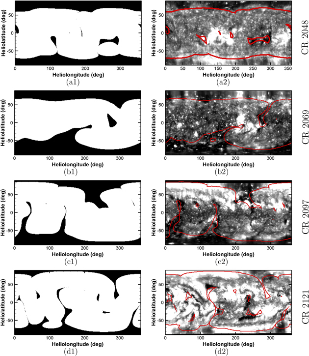
Figure 2. Synoptic maps of the open- (black) and closed-field (white) regions of the coronal magnetic fields from the PFSS model (left) and EUV observations (right) for CRs 2048 (a1, a2), 2069 (b1, b2), 2097 (c1, c2), and 2121 (d1, d2), with the red lines in the right column representing the simulated borders between the open and closed magnetic fields.
Download figure:
Standard image High-resolution imageFrom the comparison of the open and closed fields at 1Rs obtained from the PFSS model and our HLLEM-MHD model, we find that they are basically the same except for some minor discrepancies, such as the sizes, shapes, and positions of some CH extensions and isolated CHs. Some very small isolated CHs produced by simulations are not captured by the PFSS model. Moreover, the PFSS model produces an isolated CH centered at (θ, ϕ) = (4°, 275°) in CR 2069, while the HLLEM model obtains a CH extension at almost the same position.
In general, the sizes and distributions of various kinds of CHs vary with different solar activity phases. In Figure 2, polar CHs for all four CRs can be seen clearly in the modeled results, but the observed polar CHs are only visible for the first three CRs, and those of the last CR can only be identified in sporadic regions near both poles with the naked eye. Computed from the simulated results, the areas of CHs are 11%, 15%, 12%, and 8% of the solar surface for CRs 2048, 2069, 2097, and 2121, respectively. Obviously, the area of the open-field regions for CR 2121 is relatively small. The percentages are in good agreement with the estimations by Wang et al. (2009), who investigated the variations of the CHs and open flux from 1967 to 2009 using the PFSS model. However, the results are significantly larger than those obtained from automated CH detection using EUV observations by Lowder et al. (2014, 2017). On the one hand, the CHs from automated detection contain uncertainties from limited observation quality and tunable CH detection criteria. It is noted by Lowder et al. (2014, 2017) that the polar regions are not well covered before mid-2010 owing to the single vantage point of SOHO/EIT. With the combination of SDO/AIA and STEREO/EUVI A/B data, this polar coverage gap is reduced after mid-2010 to some extent. During the period of the second half of 2010, when both EIT and AIA-EUVI observations are analyzed, the CH area measured from AIA-EUVI observations is significantly greater than that measured by EIT observations. Caplan et al. (2016) proposed another automated CH detection scheme, which performs substantially more processing of the EUV image than Lowder et al. (2014) and uses a two-threshold method rather than a single threshold. For CR 2098, the total CH area obtained by the Caplan et al. (2016) method using AIA-EUVI observations is 7.6 × 1021 cm2, which is equal to about 12.5% of the solar surface (Linker et al. 2017). This result is larger than that of Lowder et al. (2014, 2017) and closer to our result for CR 2097. On the other hand, our modeled results tend to overestimate the coverage of CHs possibly as a result of the much coarser resolution of the spatial grid in the path-conservative HLLEM model than that in the EUV measurements or the inaccurate polar field from the GONG magnetogram. Moreover, for the simulation and the observations in CR 2048, there are no polar CH extensions. For CR 2069, both the modeled and the observed results show that there is a northern CH extension that reaches (θ, ϕ) = (−10°, 275°) and a southern one that stretches from (θ, ϕ) = (−47°, 140°) to (θ, ϕ) = (−7°, 220°). From the simulation and the observations for CR 2097, we find that the simulation well reproduces two slender observed southern transequatorial CH extensions that reach about latitude 20° and captures the northern hook-like CH extension with reasonable accuracy except for subtle differences. For CR 2121, the synthesized image gives rough descriptions of the observed northern CH extension from (θ, ϕ) = (67°, 270°) and the southern one from (θ, ϕ) = (−68°, 312°). We should note that the seemingly southern transequatorial CH extensions starting from (θ, ϕ) = (−62°, 123°) indeed consist of a series of very small disconnected open-field regions if we examine them by enlarging the panel.
As we can see, the simulations do not show any significant isolated CHs for CR 2069, but they do achieve some in basic agreement with the observations for CRs 2048, 2097, and 2121. With a few-degree differences, the simulations well capture the isolated CHs centered at (θ, ϕ) = (8°, 5°), (−17°, 266°), and (16°, 357°) for CR 2048, (21°, 90°), (7°, 311°), and (20°, 340°) for CR 2097, and (12°, 14°), (−45°, 78°), (−25°, 151°), (12°, 237°), and (−34°, 249°) for CR 2121. However, there are significant differences between the simulations and the observations for some other isolated CHs, and the simulations even miss or falsify some miniature isolated CHs, probably owing to the evolution of the solar corona within a CR and the poor discernibility of polar fields. From the above discussions, we can see that the simulations during the periods of the declining phase (CR 2048), the solar minimum (CR 2069), and the rising phase (CR 2097) are in good agreement with the observations, and there is a fairly good similarity between the simulation and the EUV image for CR 2121.
In Figure 3, we display the simulated open (black) and closed (white) regions at 1.5Rs (left column) and 2.5Rs (right column) for CRs 2048, 2069, 2097, and 2121. Combination of Figures 2 and 3 reveals that the open- and closed-field regions vary with the heliocentric distances (Linker et al. 1999). It is obvious to detect that the open-field regions increase as the heliocentric distance increases and the closed-field regions decrease to narrow bands around the magnetic neutral lines (MNLs) at 2.5Rs. The magnetic fields become almost open above 2.5Rs, which is widely accepted as the radius of the source surface in the PFSS model, although other values between 1.6Rs and 3.25Rs are sometimes adopted (Luhmann et al. 2009).
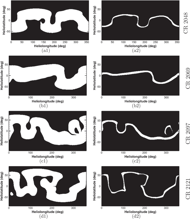
Figure 3. Simulated open (black) and closed (white) regions at 1.5Rs (left column) and 2.5Rs (right column) for CRs 2048 (a1, a2), 2069 (b1, b2), 2097 (c1, c2), and 2121 (d1, d2).
Download figure:
Standard image High-resolution image5.2. Coronal Structures near the Sun
The white-light pB images produced by the Thomson scattering from the free electrons (Linker et al. 1999; Hayes et al. 2001) are very useful to diagnose the dense coronal structures near the Sun. By blocking the light coming directly from the Sun with an occulter and creating artificial eclipses, LASCO C2 can provide the pB images routinely. In Figure 4, we present the pB images on the meridional planes of ϕ = 90°–270° observed by LASCO C2 and calculated from the modeled results for the four CRs and the corresponding 2D magnetic field topologies overlaid on the contours of the number density  . The innermost white circles of the left column are the edges of solar disks. The radii of the orange circular regions in the left column are 2.3Rs, as are those of the white circular regions in the middle column. The white regions in the right column are solar disks. It should be noted that the synthesized pB images have been enhanced by applying the technique of normalized radial graded filter (Morgan et al. 2006; Morgan & Habbal 2010; Druckmüllerová et al. 2011; Feng et al. 2015).
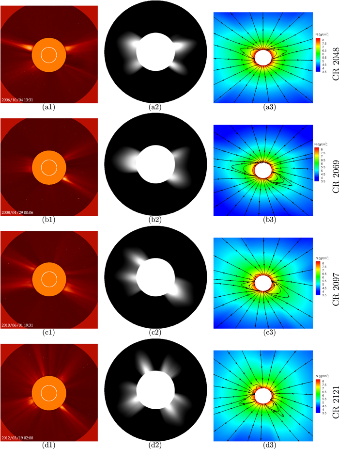
Figure 4. White-light pB images recorded from the LASCO C2/SOHO (left column) and synthesized from the results on the meridional planes of ϕ = 90°–270° of the path-conservative HLLEM-MHD model (middle column) and the 2D magnetic field topologies overlaid on the contours of the number density  on the corresponding meridional planes (right column) for CRs 2048 (a1, a2, a3), 2069 (b1, b2, b3), 2097 (c1, c2, c3), and 2121 (d1, d2, d3), respectively.
Download figure:
Standard image High-resolution imageAs shown by the previous studies (Blackwell & Petford 1966; Frazin et al. 2007; Feng et al. 2015, 2017), both bipolar streamers (also called helmet streamers) and unipolar streamers (also called pseudo-streamers) are associated with bright structures in solar coronal white-light pB images, and CHs correspond to dark regions. Bipolar streamers separate CHs of opposite magnetic polarities, while pseudo-streamers separate CHs of the same polarity (Wang et al. 2007; Riley et al. 2011; Abbo et al. 2015). When interpreted with the aid of coronal magnetic field topologies, pseudo-streamers are shown to consist of a pair of loop arcades where the like-polarity field lines converge above the cusp. In contrast, bipolar steamers are formed by helmet-like closed magnetic loops, where the opposite-polarity field lines meet above the cusp. Figure 4 reveals that the patterns of the bright structures on the selected meridional planes for the four CRs are distinct from one another. Here, for clarity, we define the central position angle (CPA) of an object on a pB image as the anti-clockwise-measured angle from the north direction to the straight line connecting the centers of the Sun and the object. From both the observed and the modeled pB images, bipolar streamers produce the broadest and brightest radially extending structures of both limbs for each CR. Their CPAs are approximately 56° and 292° for CR 2048, 86° and 231° for CR 2069, 102° and 227° for CR 2097, and 109° and 222° for CR 2121. From Figure 4, we can see that many pseudo-streamers produce less bright and relatively thin structures in the pB images whose CPAs are around 140° and 230° for CR 2048, 309° for CR 2069, 38° and 312° for CR 2097, and 38° and 265° for CR 2121. It is interesting to note that unipolar streamers are present in the pB images for all solar activity phases (Tlatov 2010). Moreover, it is the emission from the high-density region roughly at longitude 240° that results in the faint structure with its CPA being 329° in the pB images for CR 2121, which can be seen in Figure 5.
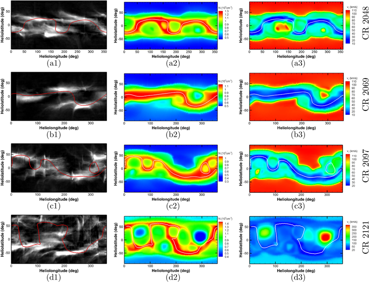
Figure 5. Synoptic maps of the white-light pB observations at the west limb from LASCO C2/SOHO (left column), number density N (106/cm3) (middle column), and radial speed vr (km s−1) at 2.5Rs (right column), with the red and the white curves representing the magnetic field neutral lines for CRs 2048 (a1, a2, a3), 2069 (b1, b2, b3), 2097 (c1, c2, c3), and 2121 (d1, d2, d3), respectively.
Download figure:
Standard image High-resolution imageFigure 5 presents the synoptic maps of the west limbs (left column) from LASCO C2/SOHO (https://lasco-www.nrl.navy.mil/carr_maps/c2/), the plasma number density N (middle column), and radial speed vr (right column) with the radial magnetic field neutral line (Br = 0) on the surface of 2.5Rs for CRs 2048, 2069, 2097, and 2121. From the left column of Figure 5, we find that the simulated MNLs are surrounded by the bright pB structures. In the middle and right columns, the neutral lines of the magnetic field are surrounded by the relatively high-density, low-speed (HDLS) flows, while both polar regions in the first three CRs are dominated by low-density, high-speed (LDHS) plasma flows. It should be noted that the bright pB structures reflect discontinuities and distortions associated with the abrupt changes of the MNLs and CMEs (Odstrcil & Pizzo 1999). Our model produces similar patterns. Concretely, in CR 2048, there are two wide flat humps from 50° to 170° and from 220° to 320° in the modeled results, and similar bulge structures appear in the observations, but with a little smaller size. For CR 2069, the dark vertical strip on the far left of the observations denotes the observation gap. The MNL is gently warped when compared with the other three CRs and roughly coincides with the solar equatorial plane. Moreover, these modeled results are similar to the solar coronal synoptic maps (Li & Feng 2018). For CR 2097, there are two small peaks centered at (θ, ϕ) = (47°, 34°) and (θ, ϕ) = (30°, 128°), a narrow trough at (θ, ϕ) = (−5°, 89°), and a broad deep trough from longitude 210° to 320° with its southernmost part reaching latitude −33°. We note that the HDLS flows extend to relatively high latitudes and cover larger areas than those in CRs 2048 and 2069. For CR 2121, the MNL has extended to very high latitudes and can be depicted as two peaks centered at (θ, ϕ) = (51°, 9°) and (θ, ϕ) = (61°, 150°) and two troughs at (θ, ϕ) = (−26°, 73°) and (θ, ϕ) = (−52°, 247°). The HDLS flows prevail at all latitudes, and LDHS flows are only present in two small regions centered at (θ, ϕ) = (28°, 59°) and (θ, ϕ) = (14°, 293°). Broadly speaking, the Carrington maps of pB obtained from LASCO C2/SOHO verify the modeled results to some extent.
It is instructive to consider the influence of the heating terms on the modeled results. In our numerical simulations, such a heating function in Equation (3) is found to have almost no significant effect on the locations of the photospheric boundaries between the open- and closed-field regions. However, our general impression of using such a heating function with θb indeed influences the solar wind speed distributions. As an example, we compare the simulated results of the solar wind speed at 2.5Rs during CR 2097 for two cases. The first case uses the heating function with the same  as Equation (4), while the second one employs the heating function with
 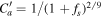 , which is independent of θb. Figure 6 presents the synoptic maps of the solar wind speed at 2.5Rs during CR 2097 for the two cases. From the figure, we find that the inclusion of θb (left) in the heating function gives relatively higher speeds in polar regions and steeper variations from low- to high-speed solar wind streams. On the other hand, the effect of the consideration of θb on the solar wind speeds may vary for the time intervals investigated, i.e., the synoptic data of the photospheric magnetic field. Quantitatively analyzing the effects of various parameters is a formidable task and needs further considerations.
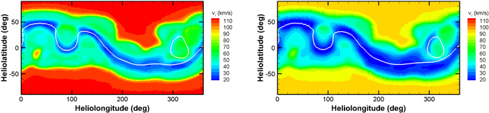
Figure 6. Synoptic maps of radial speed vr (km s−1) at 2.5Rs during CR 2097 for Case 1 (left) and Case 2 (right), with the white lines denoting the magnetic neutral lines (Br = 0).
Download figure:
Standard image High-resolution image5.3. Coronal Evolutions from 2.5Rs to 20Rs
Figure 7 presents the 3D views of the neutral surfaces of magnetic field on the meridional plane of ϕ = 0°–180° and the corresponding coronal magnetic field configuration achieved by the HLLEM-MHD model for CRs 2048, 2069, 2097, and 2121 from left to right. The central spherical surfaces are color-coded by the radial magnetic field Br on the bottom boundary. The figure gives us direct impressions to the modeled 3D topologies of the neutral surfaces of the magnetic field. For the four CRs investigated, the tilt direction of the magnetic neutral surface (MNS) is consistent with that of the helmet streamer. Specifically, for CR 2048, both sides of the MNS stretch southward, and, in almost the same directions, there are two broad helmet streamers in the corresponding image of the coronal magnetic structure. For CR 2069, which is around the solar minimum, the MNS is nearly in the heliospheric equatorial plane and has a little latitudinal excursion. Meanwhile, the coronal magnetic field is relatively simple with the large closed loops that connect the northern and southern midlatitude regions and form two helmet streamers at the east and west limbs. Besides, the magnetic field lines located near the equator at large distances map back to higher latitudes at the solar surface, which is similar to the illustration in Linker et al. (1999). Compared with CR 2069, the tilt angle of the MNS for CR 2097 is larger and the footpoints of the large closed loops can reach higher latitudes. As for CR 2121 near the solar maximum, the MNS is highly warped with complex current sheet structures (Crooker et al. 1993) and appears to be a twofold topology (Hu et al. 2008; Pinto & Rouillard 2017), which is probably attributed to high-order components of the coronal magnetic field (Hu et al. 2008). Meanwhile, seen from the coronal magnetic field configuration, bipolar and unipolar streamers are present in high latitudes, large CHs are rooted in the areas close to the equator, and the footpoints of closed magnetic field lines are scattered at almost all latitudes. The evolution of the MNSs and the coronal magnetic configurations for the four CRs are compatible with the conclusion that the current sheet resides at the lowest heliographic latitudes at the solar minimum and tilts to the highest latitudes at the solar maximum (Zhao & Fisk 2011).
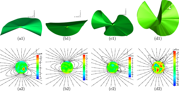
Figure 7. Three-dimensional representations of the simulated neutral surfaces of magnetic field (top row) and 3D modeled magnetic field lines (bottom row) on the meridional plane of ϕ = 0°–180° with the central spherical surfaces color-coded by the radial magnetic field Br (Gauss) on the bottom boundary for CRs 2048 (a1, a2), 2069 (b1,b2), 2097 (c1, c2), and 2121 (d1, d2).
Download figure:
Standard image High-resolution imageFigure 8 shows the 2D magnetic field lines overlaid on the contours of the radial speeds vr on the meridional plane of ϕ = 90°–270° for CRs 2048, 2069, 2097, and 2121. The meridional planes of these images are the same as those of the middle and right columns of Figure 4, but with larger regions. The pseudo-streamers are too small to be displayed in Figure 8, but they are presented clearly in Figure 4. From Figures 2 and 8, we can see that solar wind with the highest velocities comes from polar CHs or their extensions (Levine et al. 1982; Neugebauer et al. 1998; de Toma 2011), while the origin of the slow wind is an open issue, which may be associated with the boundary between the open- and closed-field regions, the streamer belt regions, the quiet areas, and the active regions (Antonucci et al. 2000; McComas et al. 2008; Riley et al. 2012; Luhmann et al. 2013; Poletto 2013; Abbo et al. 2016; Kilpua et al. 2016; Feng et al. 2017). Moreover, for CRs 2069 and 2097, the high-speed solar wind flows in low latitudes, different from those in the polar regions, are often contributed by polar CH extensions or isolated mid- and low-latitude CHs (Zhao & Fisk 2011). Furthermore, the slow and fast streams mix in latitude for CR 2121, and the slow wind is only present in low latitudes at the solar minimum, which is in agreement with the previous studies (Pinto & Rouillard 2017).
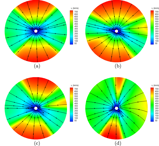
Figure 8. Two-dimensional magnetic field lines overlaid on the contours of the radial speeds vr (km s−1) in the meridional plane of ϕ = 90°–270° from 1Rs to 20Rs for (a) CR 2048, (b) CR 2069, (c) CR 2097, and (d) CR 2121.
Download figure:
Standard image High-resolution imageFigure 9 displays the location of the Alfvén surfaces (ASs) in the meridional plane of ϕ = 90°–270°, together with the contours of the radial speeds vr. From the figure, we can see that the shapes of the ASs are not spherical and the positions of the loci of ASs are higher in the polar CHs and lower in the coronal streamer. As for CR 2048, the image indicates that the AS in the polar CHs lies between 6.9Rs and 9Rs and between 3.1Rs and 11.3Rs in the coronal streamer. For CR 2069, the AS lies between 5.3Rs and 8Rs in the polar CHs and between 3.3Rs and 11.2Rs in the streamer regions. For CR 2097, the AS ranges from 6.3Rs to 8.2Rs in the polar CHs and from 2.9Rs to 10.9Rs in the streamer regions. In CR 2121, the AS ranges from 5Rs to 10.4Rs in the polar CHs and from 3.2Rs to 12.1Rs in the streamer regions. The wide varying ranges of the ASs are also pointed out in former references (Sheeley et al. 2004; Zhao & Hoeksema 2010; DeForest et al. 2014; Goelzer et al. 2014; Cohen 2015; Feng et al. 2015; Pinto & Rouillard 2017).
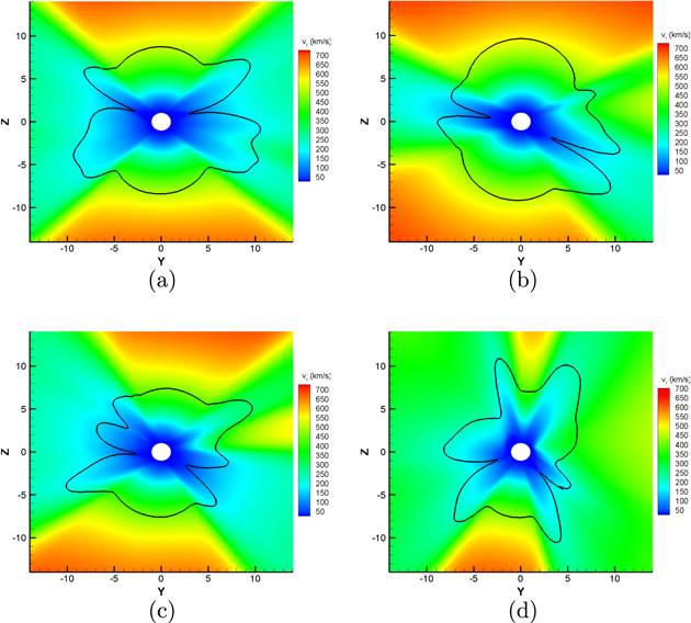
Figure 9. Two-dimensional contours of the radial speeds vr (km s−1) in the meridional plane of ϕ = 90°–270°, with the black lines representing the locations where the Alfvénic Mach number is 1 for (a) CR 2048, (b) CR 2069, (c) CR 2097, and (d) CR 2121.
Download figure:
Standard image High-resolution imageWe present the synoptic maps of temperature T, number density N, and radial speed vr at 20Rs in Figure 10 for CRs 2048, 2069, 2097, and 2121 to show the radial evolution of plasma parameters. Comparing Figures 5 and 10, we can see that the radial speeds increase and number densities decrease substantially. Figure 10 exhibits similar distributions of the HDLS and LDHS at 20Rs to those at 2.5Rs shown in Figure 5. It should be noted that the same coronal structures at 20Rs shift leftward slightly in longitude compared with those at 2.5Rs. In addition, the distributions of plasma temperature T are positively correlated with the radial wind speeds, while the distributions of plasma density and solar wind speed anti-correlate (Elliott et al. 2012; Pinto & Rouillard 2017).
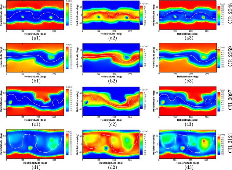
Figure 10. Synoptic maps of temperature T (105 K) (left), number density N (103/cm3) (middle), and radial speed vr (km s−1) (right) at 20Rs, with the white lines denoting the magnetic neutral lines (Br = 0) corresponding to CRs 2048 (a1, a2, a3), 2069 (b1, b2, b3), 2097 (c1, c2, c3), and 2121 (d1, d2, d3).
Download figure:
Standard image High-resolution imageFigure 11 presents the radial profiles of the number density N and radial speed vr from 1Rs to 20Rs at different locations. The positions presented for each CR are specially selected to show the significant difference between the fast and slow solar winds. The data for the high- and low-speed coronal plasma flows are sampled along the radial lines starting from open- and closed-field regions at the base of the corona, respectively. As a result, we choose (θ, ϕ) = (66°, 90°) and (180°, 90°) for CR 2048 (first column), (θ, ϕ) = (81°, 90°) and (180°, 90°) for CR 2069 (second column), (θ, ϕ) = (81°, 90°) and (180°, 90°) for CR 2097 (third column), and (θ, ϕ) = (90°, 90°) and (171°, 90°) for CR 2121 (last column). In the figure, the solid lines represent the variations of low-speed plasma flows, and the dashed lines stand for the variations of high-speed plasma flows. From 2.5Rs to 20Rs, the plasma number densities reduce roughly from 105.6 to 102.7 cm–3 for high-speed flows and from 106.1 to 103.4 cm–3 for low-speed flows in all the simulated profiles, while the flow speeds increase roughly from 90 to 700 km s−1 for high-speed flows and from 20 to 270 km s−1 for low-speed flows in all four CRs. The variations of the plasma flow speeds from 2.5Rs to 20Rs are consistent with the results derived from LASCO C2 and C3 measurements (Wang et al. 1998; Porfir’eva et al. 2009).
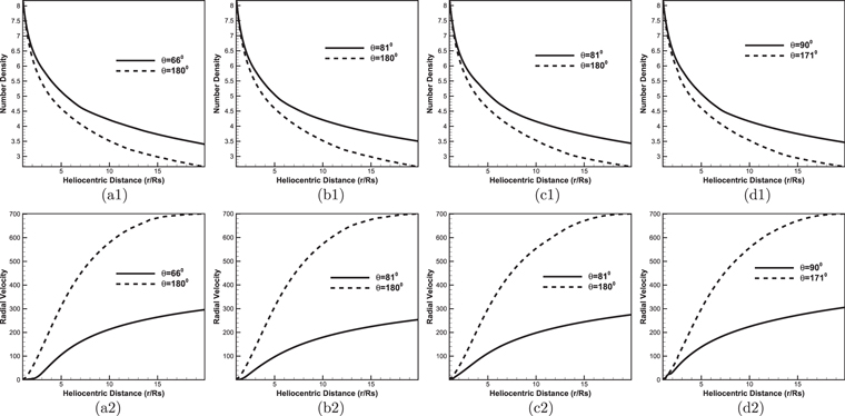
Figure 11. Radial profiles of the number density  (top row) and radial speeds vr (km s−1) (bottom row) along the different radial directions for CRs 2048 (a1, a2), 2069 (b1, b2), 2097 (c1, c2), and 2121 (d1, d2).
Download figure:
Standard image High-resolution image5.4. Comparisons between the Mapped OMNI Observations and Modeled Results
To further verify the modeled results, we show the comparisons of calculated radial velocities and polarities of the radial magnetic field Br at 20Rs with the corresponding mapped measurements obtained from the data in the OMNI archive (King & Papitashvili 2005) in Figure 12. The solid lines in the top panels are the simulated results from the HLLEM-MHD model, and the dashed lines stand for the mapped observations. For the bottom panels, asterisks denote the mapped polarities of the radial magnetic field Br, and the solid lines represent the modeled results. The mapped observations are obtained by using the ballistic approximation (Yang et al. 2012), in which the longitudinal differences are computed from the time interval for plasma flow to travel from 20Rs to 1 au. The ballistic approximation is a half-measure to remedy the deficiency that there are no in situ solar wind observations in our computational domain.
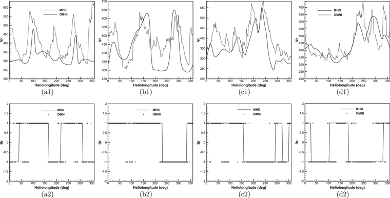
Figure 12. Temporal profiles of the radial speed at 20Rs obtained from the HLLEM-MHD model and the mapped in situ OMNI observations (top row), and the modeled and observed polarities of the radial magnetic field Br (bottom row), with “−1” symbolizing the field lines pointing to the Sun and “1” the field lines directed away from the Sun for CRs 2048 (a1, a2), 2069 (b1, b2), 2097 (c1, c2), and 2121 (d1, d2).
Download figure:
Standard image High-resolution imageFor CR 2048, the model reproduces all the troughs and two peaks at longitudes 102° and 271° but misses the peaks at longitude 190° and 352°. The omission of the peak at longitude 352° may result from the discontinuity near the longitude of 360° in the magnetic synoptic map due to the evolution after a CR. As for CR 2069, the observed peaks and troughs are basically captured by the simulation except that there are speed differences of about 100 km s−1 between the observation and the simulation for the peak at 25° and the trough at 224°. In CR 2097, the simulation achieves almost the same observed profiles after longitude 150° and the slow plasma flow from longitude 0° to 150°, where the model failed to capture the fluctuations. For CR 2121, the simulation basically replicates the observed profiles, but the modeled maxima of the narrow peaks are significantly smaller than the observed ones. After simple calculations according to the data presented in the bottom panels of Figure 12, we can obtain the hit ratios of the modeled polarities of the radial magnetic field to the observed ones. The hit ratios are 74.2%, 88.4%, 74.5%, and 72.5% for CRs 2048, 2069, 2097, and 2121, respectively, which shows that the simulations are basically consistent with the observations for the polarities of the magnetic fields.
Examining Figure 12, we find that there are two leading types of discrepancies between the observations and the simulations: inaccurate magnetic sector boundaries in the polarity panels and misaligned rising fronts and declining slopes in the speed panels. Several factors contribute to these discrepancies, such as data gaps of photospheric magnetic field in both polar regions, the coronal evolution within the selected CRs, the imperfect treatment of coronal heating, and CMEs.
As we know, photospheric magnetic field measurements can only be obtained either from the ground-based observatories or from the spacecraft near Earth. Therefore, polar fields are not well resolved or periodically missing owing to the projection effect and the variation in the solar B-angle (Arge & Pizzo 2000; Sun et al. 2011). Wang et al. (2009) and Yang et al. (2011) pointed out that polar fields can significantly affect the loci of the heliospheric current sheet (HCS). Furthermore, the empirical coronal heating function employed in the paper is highly dependent on the topology of HCS at r = 2.5Rs. The combination of polar gap in photospheric magnetic fields and the imperfect coronal heating function leads to unneglectible errors of the temporal profiles of the solar wind and wrong polarities of the interplanetary magnetic field. What is more, the solar corona during solar maxima or rising phases often undergoes rapid changes within a CR (McComas et al. 2000; Feng et al. 2012b), which can also deteriorate the simulated results. Additionally, simulations for the steady solar wind exclude CMEs that can disturb the solar wind from several hours to 2–3 days. According to the CME list available at http://www.srl.caltech.edu/ACE/ASC/DATA/level3/icmetable2.htm, the CME recorded by LASCO C2/SOHO at 1406 UT on 2010 May 24 produced the abrupt rising at longitude 300° of CR 2097. The halo CMEs at 0024 UT on March 7 and at 1736 UT on 2012 March 13 lead to the sudden increases in the solar wind speed at longitudes 330° and 260° of CR 2121. The CME on March 7 was also pointed out by Shugay et al. (2014).
5.5. Relative Divergence Errors
Figure 13 displays the evolutions of the average relative divergence error for the four CRs. Here the average relative divergence error is defined as 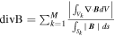 , with M being the total number of cells in the computational domain (Powell et al. 1999; Pakmor & Springel 2013; Mocz et al. 2014; Zhang & Feng 2016). From the image, we can see that the average relative divergence errors increase rapidly in the first 10 hr, then decrease from 10 to 20 hr, and finally tend to keep stable until the end of the simulations (Zhang & Feng 2016). The final average relative divergence errors are almost 2.5 × 10⁻⁴ for CRs 2048, 2069, and 2097 and 3.5 × 10⁻⁴ for CR 2121. As far as the relative divergence error is concerned, the performance of the HLLEM model can be comparable to some commonly used models (Duffell & MacFadyen 2011; Pakmor et al. 2011; Gaburov et al. 2012; Pakmor & Springel 2013; Zhang & Feng 2016).
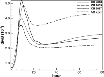
Figure 13. Temporal evolution of the average relative divergence error for CRs 2048 (solid line), 2069 (dashed line), 2097 (dotted line), and 2121 (dot-dashed line).
Download figure:
Standard image High-resolution image6. Conclusion
In this paper, we implemented a novel path-conservative formulation of the HLLEM Riemann solver in spherical coordinates to nonconservative G-EGLM hyperbolic MHD systems that describe solar wind plasma and magnetic field. The proposed scheme can include an arbitrary number of intermediate characteristic fields, which can be achieved by a generalization of the diagonal matrix  derived from a simple and general expression. In principle, the path-conservative formulation of the HLLEM scheme can accommodate any intermediate wave as long as its eigenstructure is known. Additionally, since the HLLEM Riemann solver is built on top of the path-conservative formulation of the HLL method, it naturally inherits the good positivity properties, the entropy enforcement, and robustness of the underlying HLL scheme. Different from the HLL scheme, linearly degenerate intermediate waves ensure that slowly moving linearly degenerate inner characteristic fields are well preserved or minimum smeared.
The present HLLEM scheme for the G-EGLM MHD solar wind model Equations (1) is established by using an FVM with the “8(HLLEM)+1(LF),” “7(HLLEM)+2(analytic),” or “9(HLLEM)” nonlinear Riemann solver introduced in Section 4.2, the one-step MUSCL-type time integration, and the logarithmic spacetime reconstruction (8) or the minmod piecewise linear spacetime reconstruction (9). We have tested all the cases described above and found that they are almost equally accurate, robust, and stable with a satisfactory time-step restriction. It should be noted that the numerical results displayed in Section 5 are obtained by using an FVM with the “8(HLLEM)+1(LF)” nonlinear Riemann solver.
With the path-conservative HLLEM-MHD model, we simulate the large-scale solar coronal structures for CRs 2048, 2069, 2097, and 2121. The modeled results are presented in Section 5. The path-conservative HLLEM-MHD model achieves many large-scale solar coronal structures that are in reasonable agreement with the observations. The distributions of open and closed fields have been well revealed in the simulated results. Polar CHs and isolated CHs have also been roughly caught by the model. Additionally, both the helmet streamer belts and pseudo-streamers have been captured to a relatively satisfactory extent. Besides, the mapped OMNI in situ measurements are basically consistent with the simulated results. Finally, the average relative divergence errors are controlled in the relatively satisfactory range during all the simulations. However, there are a few discrepancies between the simulations and the observations. There are some biases for the sizes of the CHs between the modeled results and the observations, and some small details of CHs have not been reproduced in our model. Moreover, the temporal variations of the magnetic polarities and radial velocities have some misalignments with the corresponding mapped observations. To sum up, the path-conservative HLLEM-MHD model exhibits the capability of producing the large-scale solar coronal structures.
Further improvements are needed for the path-conservative HLLEM model to better simulate the solar wind from the Sun to Earth or beyond. Near-realistic coronal heating functions should be developed and be exploited to reduce the artificial tunable parameters in the heating functions. The future missions will provide photospheric magnetic field measurements from the perspectives different from Earth (Gopalswamy et al. 2011; Vourlidas 2015; Pevtsov et al. 2016; Petrie et al. 2018), which will enhance the quality of photospheric magnetic fields and improve the accuracy of the model. Data-driven modeling (e.g., Feng et al. 2012a, 2015, 2017; Yang et al. 2012; Hayashi 2013; Li & Feng 2018) will promisingly help the model to better capture the dynamical solar and interplanetary features. These topics will be left for our future considerations.
The work is jointly supported by the National Natural Science Foundation of China (grant nos. 41531073, 41731067, 41574171, and 41504132) and the Specialized Research Fund for State Key Laboratories. This work utilizes data obtained by the Global Oscillation Network Group (GONG) program, managed by the National Solar Observatory, which is operated by AURA, Inc., under a cooperative agreement with the National Science Foundation. The data were acquired by instruments operated by the Big Bear Solar Observatory, High Altitude Observatory, Learmonth Solar Observatory, Udaipur Solar Observatory, Instituto de Astrofísica de Canarias, and Cerro Tololo Inter-American Observatory. The STEREO/SECCHI data are produced by a consortium of the NRL (US), LMSAL (US), NASA/GSFC (US), RAL (UK), UBHAM (UK), MPS (Germany), CSL (Belgium), IOTA (France), and IAS (France). The SOHO/LASCO data used here are produced by a consortium of the Naval Research Laboratory (USA), Max-Planck-Institut für Aeronomie (Germany), Laboratoire d’Astronomie (France), and the University of Birmingham (UK). SOHO is a project of international cooperation between ESA and NASA. The OMNI data are obtained from the GSFC/SPDF OMNIWeb interface at http://omniweb.gsfc.nasa.gov. The work was carried out at the National Supercomputer Center in Tianjin, China, and the calculations were performed on TianHe-1 (A).
Appendix A: Modified Eigensystem
For simplicity, we use the same letters l and r to denote eigenvectors in both conservative variables U = (ρ, ρvr, ρvθ, ρvϕr sin θ, E1, Br1, Bθ1, Bϕ1, ψ) and primitive variables W = (ρ, vr, vθ, vϕ, p, Br1, Bθ1, Bϕ1, ψ) by differing them with their arguments, that is, l(U) and r(U) stand for the left and right eigenvectors in conservative variables U, and l(W) and r(W) the left and right eigenvectors in primitive variables W. Here, only the eigenvalues and eigenvectors corresponding to the matrix Ar (U) in the r-direction are derived. First, we write out the eigensystem in primitive variables W. For convenience, cfr and csr denote the fast and slow magnetosonic speeds in the r-direction
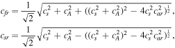
where cs  and cA
  are the sound and total Alfvénic speeds, respectively. car
  is the Alfvénic speed in the r-direction. As said above, the parameter ch is often chosen to be the largest propagation speed in the computational domain

Here cfr, cfθ, and cfϕ are the fast magnetosonic speeds in the r-, θ-, and ϕ-directions. The eigensystem in primitive variables W of the Galilean invariance EGLM in the r-direction is listed as follows:


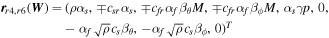
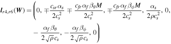

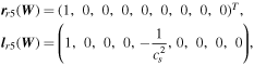
where
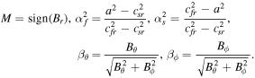
The eigenvectors given above are orthogonal, additionally, since αf, αs, βθ, and βϕ all lie between zero and one, and the eigenvectors are all well formed once these four parameters are defined. The difficulties in defining these occur when  , in which case βθ and βϕ are ill-defined, and when
  and
and  , in which case αf and αs are ill-defined. The first case is fairly trivial: βθ and βϕ represent direction cosines for the tangential component of the B-field, and in the case of a zero denominator, we only should choose
  (Brio & Wu 1988; Zachary & Colella 1992; Roe & Balsara 1996; Cargo & Gallice 1997; Barth 1999; Powell et al. 1999; Wesenberg 2002, 2003; Mignone & Tzeferacos 2010; Mignone et al. 2010; Susanto et al. 2013). An approach for the case in which αf and αs are ill-defined has been outlined in detail by Roe & Balsara (1996). In this case, they have shown multiple solutions in Roe & Balsara (1996) for the linearized Riemann problem not affecting the values for the interface fluxes. Serna (2009) applied another approach for the ill-defined αf and αs, choosing
  . That is to say,
- I.If
 , then , and , .
 - II.If and , then and , .
- III.If and , then and .


If Br tends to zero, then car = 0 and csr = 0, lr3(W) ∥ lr7(W), and lr4(W) ∥ lr6(W). In this situation, a set of new eigenvectors need to be found. From the original eigenvectors in the rows of Lr(W), we can easily see that lr1(W), lr2(W), lr5(W), lr8(W), and lr9(W) are still valid eigenvectors remaining linearly independent of each other, while lr3(W), lr7(W), lr4(W), and lr6(W) vanish. To find other valid eigenvectors, we use the original forms of the faded eigenvectors by taking account of their linear combinations and then taking the limit  . Following this line, the consideration of the difference between lr7(W) and lr3(W) results in a valid eigenvector:
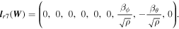
Scaling the summation of lr4(W) and lr6(W) and taking the limit  , one gets another eigenvector,
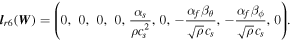
Since the third and fourth components of all the eigenvectors available so far are zeros, the most natural choices of the remaining two eigenvectors linearly independent of the other are
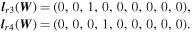
Thus, in the case of Br = 0, the newly obtained matrix Lr(W) reads as follows:
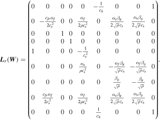
Following the same way, we obtain the newly right eigenvectors:
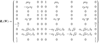
For conservative variables U, the eigenvalues are all the same, but the eigenvectors are obtained by converting to their conservative forms via the transformation matrix  and
and  :
:
where transition matrices between the conservative and primitive variables  and
and  are
are
with 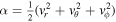 and ζ = γ − 1.
Appendix B: Calculation of the Intermediate State

Dumbser & Balsara (2016) provided a detailed procedure about how to obtain the intermediate state  . According to Equation (14) of Dumbser & Balsara (2016), the final equation for the intermediate HLL state
  reads
reads
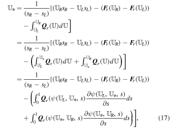
where the path  between two generic states
  and
and  is a Lipschitz continuous function that satisfies
  and
and  . Here we choose the straight line segment between two arbitrary states
  and
and  as previous authors do (e.g., Castro et al. 2008, 2013, 2016; Abgrall & Karni 2010; Dumbser & Toro 2011a, 2011b; Nguyen & Dumbser 2015; Dumbser & Balsara 2016; Leibinger et al. 2016; Sánchez-Linares et al. 2016; Feng et al. 2017):

Then,
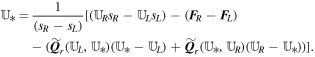
In the context of path-conservative schemes, the matrix  can be computed directly based on the path integral, which can be carried out with the Gauss–Legendre quadrature rule (e.g., Castro et al. 2008; Nguyen & Dumbser 2015; Leibinger et al. 2016; Dumbser & Balsara 2016):
Here, q is the number of quadrature points and sℓ are the Gauss–Legendre quadrature points with associated weights ωℓ on the unit interval [0, 1]. Hereafter, we employ the classical three-point Gauss–Legendre rule,  , as formerly suggested (Dumbser & Toro 2011a, 2011b; Dumbser & Balsara 2016).
In order to obtain  , we need to solve the above nonlinear Equation (17). In the case of the HLLEM method for nonconservative systems, Dumbser & Balsara (2016) provided three practical solution methods with very rapid iteration convergence. In these methods, an initial guess for
  , denoted by
  , is provided by approximating the path from
  to
to  via the following straight segment:
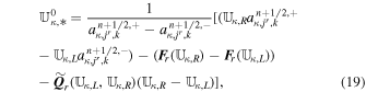
with κ ∈ {im, ip}. Here, for being self-contained, we restate these methods for our purpose.
In the first method described by Equation (20), we can compute  by using the initial guess (19) in the following simple iterative scheme:
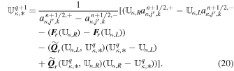
In the second method given by Equation (22), first define a nonlinear function
and then use a quasi-Newton-type iterative scheme to solve
with  as given by Equation (19) and
  .
.
The third method formulated in Equation (23) below is presented for a fully consistent HLLEM formulation in the nonconservative case, which is the same as Equation (20) in theory. In the HLLEM scheme (12), the piecewise linear variation of the wave structure has no influence on the resulting HLL state  , which can be seen as a simplifying assumption in the case of general nonconservative hyperbolic systems. In Appendix A of Dumbser & Balsara (2016), the authors further assume that the piecewise linear structure of the Riemann problem has two additional jump discontinuities
  and
and  , with
  between
  and
and  at the left speed sL and
  between
  and
and  at the right speed sR:


In the case of the HLLEM method for nonconservative systems, the fully consistent relation for the star state  can be obtained iteratively as follows:
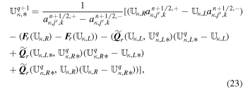
with
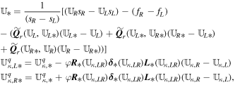
and  as given by Equation (19). However, the HLL fluctuation in Equation (12) for a fully consistent HLLEM formulation under the nonconservative case now becomes
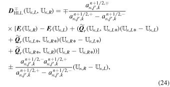
which is slightly different from that of Equation (10) owing to two additional jump discontinuities  and
and  . It should be noted that
  in Equation (12) can also take the same form as Equation (24), and the same procedure of obtaining
  described by Equation (23) works for the completion of Equation (12).