Abstract
The HH80-81 system is one of the most powerful jets driven by a massive protostar. We present new near-infrared (NIR) line imaging observations of the HH80-81 jet in the H2 (2.122 μm) and [Fe ii] (1.644 μm) lines. These lines trace not only the jet close to the exciting source but also the knots located farther away. We have detected nine groups of knot-like structures in the jet including HH80 and HH81 spaced 0.2–0.9 pc apart. The knots in the northern arm of the jet show only [Fe ii] emission closer to the exciting source, a combination of [Fe ii] and H2 at intermediate distances, and solely H2 emission farther outwards. Toward the southern arm, all the knots exhibit both H2 and [Fe ii] emission. The nature of the shocks is inferred by combining the NIR observations with radio and X-ray observations from the literature. In the northern arm, we infer the presence of strong dissociative shocks, in the knots located close to the exciting source. The knots in the southern arm that include HH80 and HH81 are explicable as a combination of strong and weak shocks. The mass-loss rates of the knots determined from [Fe ii] luminosities are in the range ∼3.0 × 10⁻⁷–5.2 × 10⁻⁵ M⊙ yr−1, consistent with those from massive protostars. Toward the central region, close to the driving source of the jet, we have observed various arcs in H2 emission that resemble bow shocks, and strings of H2 knots that reveal traces of multiple outflows.
Original content from this work may be used under the terms of the Creative Commons Attribution 4.0 licence. Any further distribution of this work must maintain attribution to the author(s) and the title of the work, journal citation and DOI.
1. Introduction
Mass accretion followed by the ejection of material via jets/outflows is an inevitable process during the early stages of star formation. The latter is essential for the removal of excess angular momentum from the system (Pudritz & Norman 1986; Klare & Camenzind 1990). The impact of these supersonic jets on the ambient medium results in the formation of shocks (Hollenbach 1997; Suzuki-Vidal et al. 2015). Studies have shown that the shocked plasma is rich in forbidden line emission ([Fe ii], [Si ii], [Ne ii], [O i]) in the optical and infrared wavelengths (Stapelfeldt et al. 1991; Nisini et al. 2005; Dionatos et al. 2009; Sacco et al. 2012). These lines can assist us in developing a better understanding of the physical parameters of the jet and its dynamics (Lavalley et al. 1997; Bacciotti & Eislöffel 1999). Although high-velocity jets from young stellar objects (YSOs) produce shock-excited optical nebulae at large distances called Herbig–Haro (HH) objects, a search for jet signatures closer to the YSO could help us probe the inner regions. This in turn is essential for the comprehension of jet launching and collimation mechanisms from protostars. Most YSOs are embedded within their molecular clouds, causing these innermost regions to be highly obscured from our direct view in optical wavelengths. They can, therefore, be best studied at infrared and radio wavelengths (Bally et al. 2007; Anglada et al. 2018).
Generally, jets are observed to be in the form of a chain of knots rather than continuous emission. Broadly, two hypotheses have been proposed to understand the formation mechanism of knots. In the first scenario, these knots could be formed due to oblique shocks that develop from hydrodynamic, magneto-hydrodynamic (MHD), or thermal instabilities. Simulations and laboratory studies have shown that MHD instabilities could result in jet flow variability since the launch of jets occurs through magneto-centrifugal processes (Lebedev et al. 2005; Huarte-Espinosa et al. 2012). In the alternate hypothesis, the variability in the jet flow could also be a result of time variability in the accretion disk (Hartigan et al. 1995). This time variability could cause episodic ejections of dense jet material that result in the observed knots. Simulations with constant ejection velocity and episodic ejections of material can produce a chain of knot-like material consistent with the observations (Lee & Sahai 2004).
Observationally, jets have been probed from the X-ray to submillimeter (Güdel et al. 2007; Plunkett et al. 2015; Fedriani et al. 2019), and embedded jets can be well probed at near-infrared (NIR) wavelengths as they provide dual advantages of lower extinction and good spatial resolution. Numerous studies have been conducted in this domain over the past years (Whelan et al. 2004; Nisini et al. 2005; Davis et al. 2006; Podio et al. 2006; Varricatt et al. 2010). The NIR spectrum is rich in atomic ([Fe ii], [S ii], [N i], etc.) as well as molecular (H2) lines (Hartigan et al. 1994; Eislöffel et al. 2000; Nisini et al. 2002; Giannini et al. 2004), with the former tracing the inner ionized jet and the latter tracing the cold postshocked molecular gas. The most important NIR lines that have been employed to trace protostellar jets are the [Fe ii] and H2 emission lines (Stapelfeldt et al. 1991; Gredel et al. 1992; Smith 1994; Davis & Eisloeffel 1995; Reipurth et al. 2000). High-resolution observations have shown that the structure of jets/outflows can be divided into two main regions: (i) inner high-velocity material close to the jet axis, and (ii) low-velocity less ionized gas near the limb of the jet/outflow (Moriarty-Schieven & Snell 1988; Schmid-Burgk et al. 1990). The NIR H2 and [Fe ii] emission lines trace distinct regions along the same jet, and provide information complementary to that of optical and radio observations. Generally, [Fe ii] emission arises from strong shocks in the inner regions close to the jet axis, while H2 is typically associated with the boundary between the jet and the ambient medium (Davis et al. 2003). Therefore, a combination of H2 and [Fe ii] imaging of a jet can provide a unique insight into the jet propagation in the molecular cloud. It is noteworthy that there have been large-scale surveys targeted on these lines (Davis et al. 2008, 2009; Froebrich et al. 2011; Lee et al. 2014).
In this study, we investigate the HH80-81 jet associated with IRAS 18162-2048 in the NIR (1–5 μm) wave bands. IRAS 18162-2048 is a massive protostar located at a distance of 1.4 kpc (Añez-López et al. 2020). The HH80-81 jet is one of the largest known Herbig–Haro jets, which is also highly collimated, extending up to 18.7 pc (Masqué et al. 2012). Proper-motion studies of the jet in radio wavelengths have measured velocities as high as 1000 km s−1 (Marti et al. 1995). The bipolar jet consists of numerous knots and the projected direction of the jet arms lie along the northeast and southwest of the protostar in the sky plane (Rodriguez et al. 1989; Girart et al. 2001). The jet extends up to HH80 in the southwest, and up to HH80N in the northeast. The morphology and kinematics of the HH80-81 jet have been well studied in optical wavelengths by Heathcote et al. (1998). These authors estimated the velocities of knots to be up to 600–700 km s−1. Spitzer observations at 8 μm exhibit a biconical outflow cavity toward the inner radio jet (Qiu et al. 2008). Multiple molecular outflows were also detected toward this region, indicating active star formation (Yamashita et al. 1989; Qiu & Zhang 2009; Fernández-López et al. 2013; Qiu et al. 2019). Toward the central region, 25 millimeter (mm) cores have been detected by Busquet et al. (2019) using the Atacama Large Millimeter/submillimeter Array (ALMA). Of these, MM1 and MM2 have been found to be the most massive and drivers of outflows in the region, with the HH80-81 jet being excited by MM1 (Busquet et al. 2019).
Here, we present NIR narrow and broadband imaging observations of a large extent of the jet (∼5 pc in projection) aimed at characterizing the type of shocks at play. The organization of the paper is as follows. The observation details are presented in Section 2 and the results are described in Section 3. The results are discussed in Section 4 and our conclusions are summarized in Section 5.
2. Observations and Archival Data
2.1. NIR Imaging Observations
We imaged the IRAS 18162-2048 region using the Wide-Field Camera (WFCAM; Casali et al. 2007) mounted on the 3.8 m United Kingdom Infrared Telescope (UKIRT). The WFCAM has four 2048 × 2048 HgCdTe Hawaii-II arrays with an optical system that provides a pixel scale of 04. This provides a total field of view of 13
5 × 13
5 per array and 0.21 deg2 for all four arrays together. The target was located in the center of one of the four arrays and the data from only that array were used in the current study. The observations were performed by dithering the target to nine positions on the array and a 2 × 2 microstepping was done. The resulting mosaics have an image scale of 0
2 pix−1. Observations were carried out using the NIR broadband J, H, K filters and the narrowband H2 and [Fe ii] filters. The narrowband H2 filter is centered at λ = 2.122 μm and the [Fe ii] line filter at λ = 1.644 μm with a FWHM of 0.021 μm and 0.028 μm, respectively. The observations were conducted between 2020 February 20 and 2021 September 20.
The preliminary reduction including the creation of mosaics was carried out by the Cambridge Astronomical Survey Unit (CASU). For the narrowband H2 and [Fe ii] filters, further reduction including continuum subtraction was carried out using the Starlink software (Currie et al. 2014). We have obtained imaging observations of H2 in four epochs and those of [Fe ii] in six epochs. The total integration time for J, H, K, H2, and [Fe ii] filters were 720 s, 360 s, 180 s, 1440 s, and 1440 s, respectively, for each epoch of observation. For each epoch, the H2 and [Fe ii] images were aligned with K- and H-band images, respectively, using WCSALIGN. Due to variations in the seeing conditions between the narrowband and broadband observations, images with smaller point-spread functions (PSFs) were smoothed to match with the FWHM of the images with larger PSFs using the task GAUSMOOTH. For continuum subtraction, a sufficient number of isolated bright point sources were selected and their flux counts from both the narrowband and broadband sky-subtracted images were calculated. The broadband to narrowband flux ratio was then computed. For each imaging observation in an epoch, the broadband image was scaled using the average value of the ratio of these fluxes and subtracted from the narrowband image to obtain the continuum-subtracted image for that epoch. The continuum-subtracted images of all the epochs were averaged to obtain the final image.
The flux calibration of the continuum-subtracted images was carried out using the H- and K-band flux densities of isolated point sources in the field. For this, we first interpolated the broadband H- and K-filter flux densities of a few isolated point sources to the central wavelength of the narrowband filters. These flux densities were multiplied by the FWHM of the narrowband filters to obtain the total fluxes. We then derived the photometry of the point sources on the normalized narrowband images to obtain the counts in ADU. This was used to estimate the flux per ADU, and this was used to scale the counts in ADU obtained from the continuum-subtracted narrowband images to estimate the fluxes. The fluxes were not corrected for extinction, as the extinction value toward each knot is not known.
In addition to this, the  (3.678 μm) and
  (4.686 μm) imaging observations were carried out using the UKIRT 1–5 μm Imager Spectrometer (UIST; Ramsay Howat et al. 2004). UIST has a 1024 × 1024 InSb array. The observations were carried out using the 0
12 pixel−1 camera. The object was dithered to four positions along the corners of a square of 40″ side. The total integration time for the
 and
and  observations were 160 s and 280 s, respectively. For each setting, a dark observation was done, which was followed by the science observations. The dark-subtracted science frames were median combined to create sky flats. Frames in individual pairs were subtracted from each other and divided by the flats. This resulted in a positive and negative beam in the mutually subtracted, flat-fielded image. The final mosaic was constructed by combining the positive and negative beams.
2.2. Optical Archival Data
The optical emission from the HH80-81 jet in the filters Hα + [N ii], [S ii], and [O iii] has been imaged using the Wide Field and Planetary Camera 2 (WFPC2) on board the Hubble Space Telescope (HST). These high angular resolution images have been published by Heathcote et al. (1998). We have extracted these images from the Hubble Legacy Archive. We have employed these images to compare the morphologies of HH80 and HH81 with those from our NIR observations, in order to characterize the nature of shocks.
3. Results
3.1. Line Emission in NIR and Optical
The full length of HH80-81 jet as observed in H2 emission is shown in the central panel of Figure 1. The surrounding panels display the emission toward the jet in H2, [Fe ii], and the optical Hα + [N ii] filters in red, green, and blue, respectively, revealing the morphologies of individual knots. The details of the sizes and locations of the subimages are listed in Table 1. We observe that in the  image obtained by us, the jet displays a chain of knots extending up to 1.9 pc in the northeast and 2 pc in the southwest directions, as projected on the sky plane. Considering the inclination angle of the jet to be 56° (Heathcote et al. 1998) from the sky plane, the true extent of the bipolar jet as imaged in NIR is ∼7 pc. It is possible that there are additional knots extending farther away from this toward HH80N. We identify a total of nine new knots along the HH80-81 main jet direction and multiple arcs in H2 emission. Four knots are in the northern arm and five are in the southern arm of the jet. We assign numbers 1–9 to the knots as seen in our NIR images from north to south. The Knots 8 and 9 correspond to HH81 and HH80, respectively. We describe a few morphological features of the knots below:
- 1.Knots 1 and 2 exhibit only H2 emission, and Knot 4 is revealed in only [Fe ii] emission, while the remaining knots exhibit emission in both [Fe ii] and H2 transitions.
- 2.Knots 1–6 are elongated along the direction of the jet. Knots 7–9 appear broken and have complex morphologies.
- 3.In none of the knots, the regions corresponding to [Fe ii] and H2 emission completely overlap. In Knots 3 and 6, the [Fe ii] emission clearly lies ahead of the H2 emission along the outward jet direction; whereas, in the case of Knot 5, the reverse is seen.
- 4.The NIR line emission for Knots 8 and 9 do not coincide with optical line emission. For other knots, the optical data are not available.

Figure 1. Central panel: continuum-subtracted H2 image of the full length of HH80-81 jet. Surrounding panels: color-composite image of the individual knots of the jet in the NIR H2 emission (red), [Fe ii] emission (green), and HST optical Hα+[N ii] (blue). The HST observations were carried out only toward the knots HH81 and HH80. Various knots are enclosed in yellow boxes in the central image to show their locations. The details of the locations and sizes of the subimages are listed in Table 1. The cyan ellipses show the apertures used for the calculation of fluxes of each of the knots. The white contours in the enlarged images of the knots represent Very Large Array 20 cm data obtained from Marti et al. (1993). The magenta contours (dashed lines) show the GMRT 610 MHz emission from Vig et al. (2018). The cyan cross between knots 4 and 5 in the central figure indicates the driving source of the jet (MM1). Subknots toward HH80 and HH81 are shown as crosses and labeled according to Heathcote et al. (1998).
Download figure:
Standard image High-resolution imageTable 1. Coordinates of the Center and the Sizes of Subimages Shown in Figure 1
| Source Name | R.A.(J2000) | Decl.(J2000) | δR.A. | δDecl. |
|---|---|---|---|---|
| (α) | (δ) | (″) | (″) | |
| Knot 1 | 18:19:19.10 | −20:43:11.4 | 27.2 | 24.4 |
| Knot 2 | 18:19:17.13 | −20:44:47.2 | 27.2 | 24.4 |
| Knot 3 | 18:19:14.37 | −20:46:30.0 | 32.9 | 31.2 |
| Knot 4 | 18:19:12.97 | −20:47:02.4 | 32.4 | 39.5 |
| Knot 5 | 18:19:10.62 | −20:48:27.4 | 32.7 | 35.4 |
| Knot 6 | 18:19:08.45 | −20:50:03.9 | 24.0 | 27.7 |
| Knot 7 | 18:19:08.13 | −20:50:37.6 | 33.1 | 30.0 |
| Knot 8 (HH81) | 18:19:06.91 | −20:51:06.6 | 28.2 | 32.8 |
| Knot 9 (HH80) | 18:19:05.70 | −20:52:02.4 | 41.7 | 45.4 |
Download table as: ASCIITypeset image
The central region close to the driving source of the jet is shown in Figure 2. The Spitzer 8 μm broadband image is shown in red and the H2 emission is depicted in green. The maps are overlaid with the contours of [Fe ii] emission in orange. The association with radio emission is illustrated by contours (cyan) corresponding to the 610 MHz emission (Vig et al. 2018). We observe that the emission in H2 is widely distributed across the image, unlike the [Fe ii] emission. It is also evident that the [Fe ii] emission arises from the highly ionized inner jet close to the axis, while the mid-infrared (MIR) emission delineates the outflow cavity. Multiple bow shocks and knots are observed in H2 and the majority of this emission appears to be distributed in directions away from the HH80-81 jet axis. The radio jet is well delineated by the [Fe ii] emission.
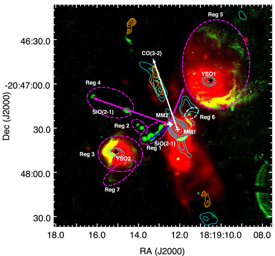
Figure 2. Two color-composite image of the central region of HH80-81 jet. The Spitzer 8 μm broadband image is shown in red and the NIR H2 emission is shown in green. The NIR [Fe ii] emission is overlaid as orange contours, and the arrows depict outflows detected in this region by Fernández-López et al. (2013) and Qiu et al. (2019). The white crosses indicate two millimeter cores that are believed to drive some of the detected outflows. The cyan contours show ionized gas at 1300 MHz (Vig et al. 2018) and the beam is shown toward the bottom left of the image as a white ellipse. The dashed ellipses (magenta) labeled as Reg 1–7 are discussed in the text. The black crosses indicate two YSOs of interest in the region.
Download figure:
Standard image High-resolution imageThe prominent H2 features in the region are:
- 1.The HH80-81 main jet: This extends along the northeast–southwest direction. The emission is seen as knots extending along the jet as well as arcs close to the central region. A detailed discussion of this jet is presented in Section 4. The catalog number of the knots associated with this jet in the Catalogue of Molecular Hydrogen Emission-Line Objects (MHOs) in Outflows from Young Stars (Davis et al. 2010) is MHO 2354.
- 2.Reg 1: This comprises a chain of five H2 knots toward the eastern side, which are enclosed within a dashed ellipse shown in Figure 2.
- 3.Reg 2: This includes two distinct H2 knots to the northeast of Reg 1.
- 4.Reg 3: This region includes arcs of H2 emission along the east and west directions on either side of a YSO (Qiu et al. 2008), as shown in Figure 2, facing inwards of the dashed ellipse of size
 . The arc toward the east is very strong in emission and with overlapping emission at 8 μm, it is seen as yellow in the figure. We note that the nebulosity at 8 μm appears well enclosed within the defined ellipse.
 - 5.Reg 4: This region shows two knots aligned northeast with respect to the central region.
- 6.Reg 5: The H2 emission shows arc-shaped patterns over a region of size. The arcs appear to surround the nebulosity observed at 8 μm. The emission to the south of the enclosed ellipse shows strong H2 emission, overlapping with 8 μm emission.
- 7.Reg 6: This region includes a knot toward the west of the central region.
- 8.Reg 7: Two faint arcs in H2 are observed facing each other within the region enclosed by the ellipse in this region.


The MHO catalog numbers of Regs 1–7 are MHO 2355−2361. A detailed description of the morphology of knots in narrow-line emission bands is presented in Appendix A.
We have estimated the integrated fluxes of knots in the narrowband H2 and [Fe ii] filters by using elliptical apertures for each of the knots, which are marked in cyan in Figure 1. The knot fluxes along with the sizes of apertures (semimajor × semiminor) used for the flux calculation are tabulated in Table 2. The H2 and [Fe ii] fluxes of the knots are in the range (0.4–5.2) × 10−14 erg s−1 cm−2 and (3.1–13.6) × 10−14 erg s−1 cm−2, respectively. Knots 1 and 2 do not have any associated [Fe ii] emission. We have also calculated the ratio of [Fe ii]/H2 emission toward knots where both are detected. This ratio is represented as  , and estimated in order to understand the nature of shock across different knots. These values are also tabulated in Table 2 and are comparable with those obtained from observational studies conducted toward other YSO jet sources (Lorenzetti et al. 2002; McCoey et al. 2004; Garcia Lopez et al. 2010). It is worthwhile to note that the extinction can be quite nonuniform along the length of the jet, and will also be affected by the inclination of the jet with respect to the line of sight. However, having stated this, we observe that
  varies widely across the knots, from 0.6 in Knot 7, suggesting relatively low excitation of [Fe ii] emission, to 12.1 in Knot 5, where [Fe ii] emission clearly dominates over the H2 emission. This clearly indicates that there is a considerable difference in the excitation conditions of the knots. We discuss this in detail in Section 4.
Table 2. Fluxes of HH80-81 Jet Knots, the Sizes of Apertures for the Flux Calculation, and the [Fe ii]/H2 Line Ratios ( )
)
| Source Name | H2 Flux | [Fe ii] Flux | Aperture Size |
 = [Fe ii]/H2 = [Fe ii]/H2
|
|---|---|---|---|---|
| (10−14 erg s−1 cm−2) | (10−14 erg s−1 cm−2) | |||
| Knot 1 | 1.7 | ⋯ a | 10 | ⋯ |
| Knot 2 | 1.3 | ⋯ a | 8 | ⋯ |
| Knot 3 | 2.6 | 4.6 | 14 | 1.8 |
| Knot 4 | ⋯ b | 11.7 | 13 | ⋯ |
| Knot 5 | 0.4 | 4.6 | 10 | 12.1 |
| Knot 6 | 0.9 | 5.2 | 5 | 6.0 |
| Knot 7 | 5.2 | 3.1 | 14 | 0.6 |
| Knot 8 | 1.5 | 7.0 | 9 | 4.7 |
| Knot 9 | 4.3 | 13.6 | 16 | 3.2 |
Notes.
a [Fe ii] emission is not detected in these knots. b H2 emission is not detected in this knot.Download table as: ASCIITypeset image
3.2. Broadband Emission in the NIR and MIR
In this section, we describe the emission from the central region in the NIR and MIR broadband filters. The emission through the NIR J, H, and K bands can be seen in Figure 3. The J-, H-, and K-band emission toward the northern extension of the jet is up to  pc. That said, toward the southern arm, the NIR J- and H-band emission is observed up to 0.2 pc, whereas the K-band emission is seen to extend up to 0.3 pc. We identify a sharp bend in the jet cavity toward the northern arm, where it is initially directed westwards but veers toward the east; see Figure 3. The most massive millimeter cores observed in this region are MM1 and MM2 (Busquet et al. 2019), which are marked in the figure. In addition, the knots and arcs that are discussed in Section 3.1 are also shown in the figure.
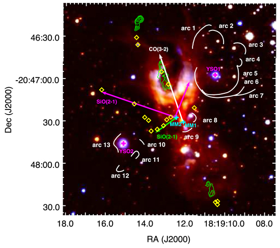
Figure 3. JHK color-composite image of the central region of HH80-81 jet. K is shown in red, H in green, and J in blue. The NIR [Fe ii] emission is overlaid as green contours, and the arrows depict outflows detected in this region by Fernández-López et al. (2013) and Qiu et al. (2019). The cyan crosses indicate two millimeter cores that are believed to drive some of the detected outflows, the magenta crosses indicate two YSOs of interest in the region, the white arcs represent the bow shocks identified in the H2 image of the central region shown in Figure 2, and the yellow diamonds show H2 knots.
Download figure:
Standard image High-resolution imageThe emission toward the central region in the  and
and  bands can be viewed in Figure 4. We note that the cavity is not seen very clearly in these images and we attribute this to the low signal-to-noise ratio images. While the
  -band image shows hints of emission toward the jet cavity near the center (see Figure 4(a)), this is not detected in the
  image. A comparison with MIR IRAC images from the space-based Spitzer mission shows the presence of strong MIR emission from the cavity walls (Figure 2). Cavities around jets in the MIR have been observed earlier and the emission has been attributed to thermal dust, which is directly heated by the central source that drives the outflow (De Buizer 2006). We observe a few point-like sources in our moderately high resolution
  and
and  images, and we identify a few of them as cores that have been observed using millimeter ALMA observations (Busquet et al. 2019). The brightest emission in the
  image is observed at ∼2000 au to the northeast of MM1. While this emission is very likely from the outflow cavity, there exists a possibility that this is a YSO, considering the point-like morphology seen in the
  image. The lack of associated millimeter emission gives more credence to the outflow cavity hypothesis, although the possibility of an evolved YSO cannot be completely ruled out. MM1 is brighter in the
  band compared to
  band, indicating that it is indeed young. We have not detected any emission associated with MM2(E) and MM2(W) in the
  band.
band.
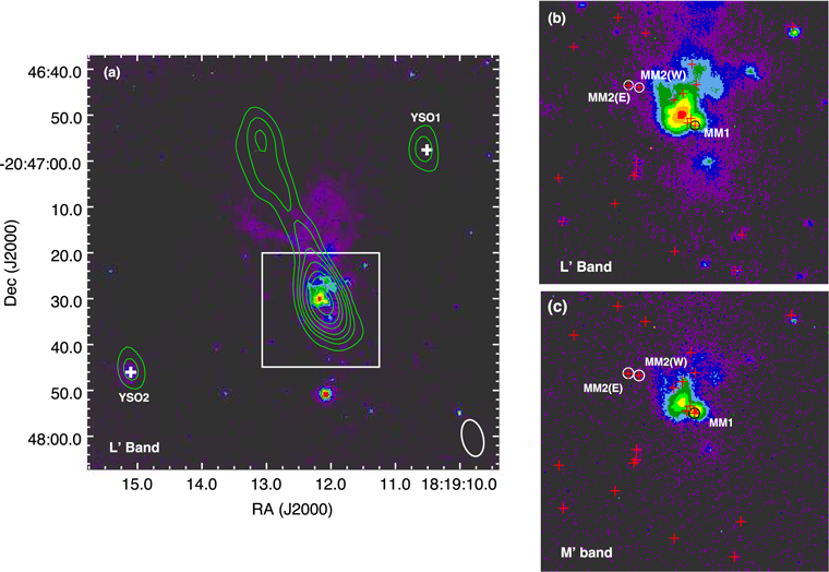
Figure 4. (a)  -band image of the central region of HH80-81 jet system obtained with UIST. The white box encloses the region of size 0
4 × 0
4 shown in (b)
 -band emission and (c)
  -band emission. The green contours represent the 20 cm radio continuum emission (Marti et al. 1993), with the beam shown as a white ellipse toward the right corner. The crosses in (b) mark the locations of millimeter cores in the central region identified by Busquet et al. (2019). The massive cores MM1 and MM2 are labeled.
Download figure:
Standard image High-resolution image4. Discussion
We have identified nine knots along the HH80-81 jet: four on the northern side and five on the southern side of the driving source, as shown in Figure 1. The morphology of the individual knots are outlined in Appendix A. In general, the excitation of 2.122 μm ν = 1−0 S(1) rovibrational line of H2 molecule can occur due to either of the following mechanisms: (i) collisional excitation in dense molecular gas that is heated up to a temperature of 2000 K by shock waves (shock-excited), or (ii) absorption of ultraviolet radiation emitted by the young star (fluorescence). In the case of HH80-81 jet, the H2 emission is observed at large distances from the central stellar source (up to 2 pc in projection on each side). Therefore, we suggest that the shock origin is a more plausible scenario than the fluorescence phenomenon. The NIR emission lines of the Fe atom are also tracers of jets (Reipurth et al. 2000; Pyo et al. 2003; Giannini et al. 2013; White et al. 2014). There are 16 low-lying energy levels in the Fe+ ion that can be easily excited. These excitations can therefore be readily achieved in shocks.
4.1. Nature of Shock in Knots
In this section, we qualitatively characterize the nature of shocks at play in each of the knots. Depending on the strength, structure, and nature of the shock generated by jets, the shocked plasma can cool via emission of atomic, molecular, or ionic lines. Thus the emission-line features can be utilized to uncover the type and nature of shocks that give rise to these emissions. Based on their physical properties, shocks can be broadly classified as (i) Jump shocks (J-type), (ii) Continuous shocks (C-type), and (iii) J-type with a magnetic precursor (Draine 1980; Flower et al. 2003). C-shocks are typically associated with velocities of ∼40–50 km s−1, low ionization of molecular gas, and strong magnetic fields. They are rich in infrared emission lines (H2, CO, H2O, etc.). J-shocks, by contrast, are faster and mostly rich in optical and ultraviolet emission lines and require high ionization levels with low magnetic field strength (Hollenbach & McKee 1989). Younger shocks typically tend to be of J-type (strong), and such shocks may eventually evolve into C-type (weak) in the presence of a strong magnetic field. A shock that has not attained thermal equilibrium could display the properties of both C- and J-type shocks. The intermediate stage in this evolution is called the J-type shock with a magnetic precursor. While spectroscopy is ideal for probing the intensities of excitation lines and hence the nature of shock at a specific location, the spatial distribution of the different excitation lines through a morphological study is equally important, as it provides strong clues about jet propagation in the ambient medium.
We utilize the H2 and [Fe ii] line images to comment on the possible nature of shocks in different knots of the HH80-81 jet. Molecular H2 is a good tracer of low-velocity (10–50 km s−1) weak molecular shocks associated with protostellar jets, i.e., shocks at low velocities (Draine 1980). In such cases, the dissociation of the H2 molecule does not occur. However, in regions of low densities, the H2 molecule remains undissociated even up to 80 km s−1 (Le Bourlot et al. 2002). Infrared H2 emission could occur either in nondissociative C-shocks or low-velocity J-shocks. This is corroborated by the fact that numerous HH flows (Schwartz et al. 1988; Lane 1989) and several CO outflows have exhibited H2 emission features tracing weaker regions of shocks with low excitation levels. J-shocks with speeds greater than 25 km s−1 are found to dissociate H2 (Kwan et al. 1977), whereas C-shocks are capable of accelerating H2 to velocities of up to 50–80 km s−1 without dissociating it (Draine 1980; Le Bourlot et al. 2002). [Fe ii] emission is widely used to understand fast and dissociative J-shocks caused by jets with velocities larger than 50 km s−1. At these velocities, the head of the bow shock can destroy the grain in which iron is locked up (Lorenzetti et al. 2002). The grain destruction releases iron in the gas phase and this is followed by ionization of the neutral iron through charge transfer reactions with ions. It is possible that J-shocks can have cooler wings, where H2 molecules are excited behind the [Fe ii] emitting region. Alternately, J-shocks with magnetic precursors can give rise to a geometry in which H2 emission is seen in front of the [Fe ii] emission (Draine 1980). The morphology of emission in shock tracers can provide a resourceful gauge to examine the interaction of the jet with the ambient medium.
In the HH80-81 jet, from the observed morphology of knots aligned along the jet, we attempt to segregate strong and weak shocks and correlate this information with signatures of C-shocks and J-shocks, as well J-shocks with magnetic precursors. In Knot 1, the elongated cavity-like H2 emission and the absence of [Fe ii] and radio emission toward this distant knot could be explicable by the weakening of the shock strength with radial distance as it moves outwards from the central source. The absence of [Fe ii] and radio emission helps to exclude a J-shock as the exciting mechanism at this knot location, and hence we propose that the shock in this knot could be a C-type shock. For Knot 2, although its morphology is different from that of Knot 1, strong H2 emission and the absence of [Fe ii] and radio emission again points toward the possibility of a C-type shock due to weakening of the shock with radial distance from the central source. The filled morphology could suggest the presence of a stronger shock. Compared to Knot 1, this shock is possibly stronger due to the smaller radial distance from the driving source. Alternatively, the emission could be from the front side of the wall cavity as mentioned earlier.
In Knot 3 the [Fe ii] emission appears to arise from the head of the bow shock and the H2 emission corresponds to the cooler wing of the bow shock, i.e., interior to that of [Fe ii] emission in the postshock cooling zone. The fast dissociative shock head of the J-shock results in the generation of Fe+ ions in the immediate postshock region, which undergoes collisional excitation and emission of the forbidden [Fe ii] transition. Behind the shock front, molecular reformation occurs due to which H2 emission is observed (Hollenbach & McKee 1989). For the H2 molecule to remain undissociated, the angle between the direction of the oblique planar shock responsible for the emission and the jet direction is expected to be less than 5°–7° for a J-type shock and 10°–15° for a C-type shock (Davis et al. 2000). In Knot 3, we find that the angle between the H2 knot and the flow direction is ∼16° and between the [Fe ii] knot and jet is ∼42°. This strongly suggests the C-type nature of the cooler wings and J-type nature of the shock head where H2 emission is missing. A similar case is observed toward Knot 6. The [Fe ii] emission is located at the bow head and H2 emission is at the cooler wings behind the shock front. This again points to the possibility of a strong dissociative J-shock with cooler wings. In Knot 4, only [Fe ii] emission is present due to the highly dissociative nature of the shock.
We observe the presence of H2 emission exterior to the [Fe ii] emission in Knot 5, and it is possible that a J-shock with a magnetic precursor can account for this scenario. The magnetic precursor causes heating and compression of the materials upstream of the shock front when the shock wave travels in a weakly ionized gas in the presence of a transverse magnetic field (Hartigan et al. 1989; Flower et al. 2003). However, here the neutrals undergo a discontinuous change of physical conditions across the shock. A low ionization fraction reduces the rate of ion–neutral collisions, resulting in weaker compression of the magnetic field. Under these low ionization conditions, if the magnetic field is strong enough the shock will possess a magnetic precursor, which compresses the magnetic field even before the shock front crosses a region. This happens in this scenario because the magnetosonic waves can propagate faster than the actual shock front (Draine 1980). Hence, the arrival of shock compression before the shock front at each location along the path of the jet flow provides favorable conditions for excitation of H2 molecules without dissociating it. This could explain the observed H2 emission in this knot. Furthermore, behind the shock compression, at the dissociating shock front, we observe [Fe ii] emission in accordance with predictions from the theory.
The Herbig–Haro objects HH80 and HH81 display complex morphologies. For HH81 (Knot 8), the H2 and [Fe ii]/optical emission appear to arise from bow shocks that are arched in a direction that is opposite to the jet propagation. The arching of the bow shock opposite to the direction of the flow can be explained by a scenario where the jet encounters a small and dense clump of material on its path (Stapelfeldt et al. 1991). The bow shock then curves in the direction opposite to the direction of the jet flow. Toward HH80 (Knot 9), multiple knot-like structures are observed. The presence of elongated H2 emission toward the eastern lateral edge of the [Fe ii] emitting region could have an origin in the wiggling or sideways motion of the jet flow (Marti et al. 1993; Eisloffel et al. 1994). An alternative explanation is provided by Noriega-Crespo et al. (1996), who introduce the grazing jet/cloud core collision scenario. This states that when the jet impacts on the molecular core at an angle, it gets deflected and moves away from the surface of impact. As the jet deflects away, the external pressure forces it back, causing the outflow to bounce back and forth while some gas slides closer to the core. This is the zone of interaction between the atomic and molecular gas, and the H2 excitation most likely arises from this region. We suggest that the back-and-forth motion of the jet could create internal shocks that are substantiated by the presence of elongated [Fe ii] emission, located closer to the jet axis than the H2 emission. The complex morphology of the entire knot could arise from a scenario where thermal instabilities develop in an optically thin jet that ultimately fragments and breaks up the shocked material (Field 1965; Hunter 1970). Proper-motion studies aimed at understanding the kinematics of these HH80-81 knots have measured velocities for all the subknots, and these lie in the range 74–916 km s−1 (Heathcote et al. 1998). The direction of velocity is different for different subknots, which supports our claim regarding fragmentation of these knots as a result of thermal instabilities. For HH80 and HH81, it is difficult to conclude the nature of shock that explains the entire complex morphology of knots using the NIR and optical alone, and it is possible that one or multiple types of shocks could be generated in the subknots.
The  value of each knot is representative of the strength of the shock generated. The Hollenbach & McKee (1989) model predicts that a [Fe ii]/H2 ratio of greater than 0.5 is indicative of high-velocity dissociative shocks. The
  values of the HH80-81 jet knots are greater than 0.5 (Table 2), thereby indicating the presence of J-type shocks throughout the length of the jet. In the case of Knot 5, which is located in the southern arm of the jet, the
  value is significantly high, due to its close proximity to the driving source. Here, the shocks are very strong and highly dissociative, thereby favoring [Fe ii] emission over H2. Similarly, the corresponding closest knot in the northern arm, Knot 4, is much stronger and dissociative, resulting in only [Fe ii] emission.
Next, we utilize the location of soft X-ray emission to discuss the plausible nature of shocks in these regions. The highly dissociative head of a J-shock, being the strongest section of the shock, is believed to be rich in UV and X-ray emissions. X-ray emission has been detected toward HH80 (subknots A, C, and G) and HH81 (subknot A) by Rodríguez-Kamenetzky et al. (2019) that has overlap with the optical emission. In addition, a scrutiny of the [Fe ii]/optical and soft X-ray images (Figure 2 in Rodríguez-Kamenetzky et al. 2019) suggests the X-ray emission to be marginally ahead of the [Fe ii]/optical emission in the outward propagating jet direction. This points toward the likely presence of a J-type shock at these locations. For the other subknots, the shock mechanisms are difficult to disentangle.
Although we have tried to understand the nature of shocks, i.e., strong (J), weak (C), or intermediate (J with magnetic precursor), based on the spatial distribution and overlap of H2 and [Fe ii] lines, it is possible that extinction effects could also play a role in regions where H2 is detected but [Fe ii] is not detected, as the former suffers lower (∼50%) extinction compared to the latter. This is discussed in detail in Section 4.2.
4.2. HH80-81 Jet Propagation
A comprehensive view of the jet reveals that toward the northern arm, the knots closer to the driving source display solely [Fe ii] and radio emission or a combination of [Fe ii], radio, and molecular H2 emission, whereas H2 emission dominates in the farther knots. The H2 emission is believed to trace the diffuse regions in outflow lobes that are not well collimated, whereas [Fe ii] and radio emission reveal the compact jet where the fast moving jet ejecta produces stronger shocks (Lorenzetti et al. 2002). This implies that [Fe ii] and radio emission trace the ejecta accelerated directly by the exciting source, whereas H2 emission arises from shocked ambient gas where the ejecta interacts with it. The [Fe ii] emission gradually diminishes with radial distance from the exciting source toward this arm. From this, we can infer that at smaller radial distances from the driving source, shocks are stronger J-type, and they appear to gradually weaken farther along the jet length.
In the southern arm, all the knots show both [Fe ii] and H2 emission. HH81 and HH80, located toward the southern extremity of the jet, are complex in nature, which we attribute to thermal instabilities associated with low densities. Overall, the nature of shocks in the knots would suggest that densities of the ambient medium are relatively lower toward the southern arm as compared to the northern arm. This is validated by the fact that optical emission from HH81 and HH80 is visible due to lower extinction. This is also in accordance with conclusions of Marti et al. (1993) that the knots in the northern arm interact with the molecular cloud, unlike the southern knots HH80 and HH81, which lie beyond the edge of the molecular cloud. A comparison of fields toward the northern and southern regions of the jet in the JHK three-color-composite image shown in Figure 5 of Appendix B indicates that the northern field displays a lower number of sources that are redder compared to those in the southern field.
In view of the fact that we detect both [Fe ii] and H2 emissions in all the knots in the southern arm, we carefully analyze the variation of the corresponding  values with radial distance. The
  values for all the knots are tabulated in Table 2. One can discern that, with an increase in radial distance from the central YSO,
  decreases from Knot 5 to Knot 9 with a sharp decline in the value at Knot 7. The decrease in
  with radial distance is likely to be due to a decrease in the strength of dissociative shocks. Such a decrease in
  with radial distance has also been observed in other jet systems (Davis et al. 2000; Lorenzetti et al. 2002; Nisini et al. 2002). In addition, the lower densities toward Knots 8 and 9 could also result in a decrease in H2 emission in these knots compared to the ones at smaller radial distances.
For each knot, we compare the NIR narrow-line observations with the radio emission from ionized gas, wherever available. We note that the knots giving rise to ionized gas emission are associated with [Fe ii] emission. However, the converse is not true, and the exceptions are Knot 5 (no 610 MHz emission) and Knot 7 where the [Fe ii] emission does not have a corresponding ionized gas emission. This is consistent with our assertion that the shock in this knot is J-type with a magnetic precursor. This is weaker than the strong J-type shock and it is highly likely that ionization of Fe is favorable against the ionization of hydrogen, as the former has a lower ionization potential than the latter. This would explain the lack of ionized gas emission as well as the presence of [Fe ii] toward this knot.
The overall geometry of the jet on a large scale shows a curved S-shape centered on the MM1 core in IRAS 18162-2048. This S-shape of the distribution of knots was first noted in radio by Marti et al. (1993). We have used NIR emission from multiple knots including those that emit in radio to confirm the curved morphology of the knot train. In addition, we note that a direct evidence of wiggling is seen in HH80 (Marti et al. 1993), where H2 is linearly elongated along the lateral edge of the jet, which provides support for a wiggling jet scenario. Similar geometries have been observed before in various other jets (Eisloffel & Mundt 1997; Gomez et al. 1997; Lorenzetti et al. 2002). Two possible scenarios can be considered: (i) the jet interacting with dense ambient medium (Lorenzetti et al. 2002), or (ii) the wiggling of the jet (Raga et al. 1993). The symmetric shape is believed to result from the wiggling of the jet due to precession (Bachiller et al. 2001; Lorenzetti et al. 2002; Takami et al. 2011). The jet precession, in turn, can be attributed to (A) the presence of a companion, or (B) an asymmetry in the accretion of the envelope into the disk. The presence of a companion could lead to (a) the precession of the accretion disk due to the tidal interactions with a non-coplanar companion, or (b) the orbital motion of the jet source around a companion in orbit with the core. In case (B), the asymmetry could be due to a large difference in the orientation of magnetic and rotation axes of the core as demonstrated by simulations (Hirano & Machida 2019). ALMA studies at a resolution of 40 mas (∼56 au) did not reveal the presence of a binary companion within the MM1 core at these separations (Busquet et al. 2019), and therefore higher-resolution studies are required to draw valid conclusions regarding the presence of a binary companion.
4.3. Knot Luminosities and Mass-loss Rates
The luminosities of knots in H2 and [Fe ii] lines are calculated using dereddened fluxes and are in the range 1031–1033 erg s−1, tabulated in Table 3. For this, we have assumed Av
= 30 mag (Davis et al. 2001) for the knots close to the central region and in the northern arm (Knots 1, 2, 3, 4, and 5). Rodríguez-Kamenetzky et al. (2019) had calculated Av
= 2.8 mag and 3.4 mag for HH80 and HH81 (Knots 8 and 9), respectively. For the knots at intermediate distances (Knots 6 and 7), we have assumed Av
= 15 mag. We note that the ratio of [Fe ii] and H2 luminosities ![$\left(\tfrac{{L}_{[\mathrm{Fe}\,{\rm\small{II}}]}}{{L}_{{{\rm{H}}}_{2}}}\right)$](https://content.cld.iop.org/journals/0004-637X/942/2/76/revision1/apjaca413ieqn35.gif) are in the range 1.4–70.0. This is higher than the values obtained for low-mass class 0 and class I YSOs for which
are in the range 1.4–70.0. This is higher than the values obtained for low-mass class 0 and class I YSOs for which ![$\tfrac{{L}_{[\mathrm{Fe}\,{\rm\small{II}}]}}{{L}_{{{\rm{H}}}_{2}}}\sim {10}^{-2}\mbox{--}{10}^{-1}$](https://content.cld.iop.org/journals/0004-637X/942/2/76/revision1/apjaca413ieqn36.gif) (Davis et al. 2003; Caratti o Garatti et al. 2006). We did not find this ratio for jets from massive YSOs in literature. We attempt to understand the observed
(Davis et al. 2003; Caratti o Garatti et al. 2006). We did not find this ratio for jets from massive YSOs in literature. We attempt to understand the observed ![$\tfrac{{L}_{[\mathrm{Fe}\,{\rm\small{II}}]}}{{L}_{{{\rm{H}}}_{2}}}$](https://content.cld.iop.org/journals/0004-637X/942/2/76/revision1/apjaca413ieqn37.gif) ratio in terms of the dynamical age and evolutionary stage of the YSO driving the jet. The dynamical timescale of the HH80-81 radio jet is ∼104 yr (Masqué et al. 2012), while the associated outflows provide an estimate of ∼106 yr (Benedettini et al. 2004). As massive objects have shorter evolutionary timescales compared to their lower-mass counterparts, this would suggest that the driving source is at a later evolutionary phase when compared to the low-mass class 0/I sources of similar dynamical ages (Barsony & Kenyon 1992; Andre et al. 2000). This indicates that the difference in
ratio in terms of the dynamical age and evolutionary stage of the YSO driving the jet. The dynamical timescale of the HH80-81 radio jet is ∼104 yr (Masqué et al. 2012), while the associated outflows provide an estimate of ∼106 yr (Benedettini et al. 2004). As massive objects have shorter evolutionary timescales compared to their lower-mass counterparts, this would suggest that the driving source is at a later evolutionary phase when compared to the low-mass class 0/I sources of similar dynamical ages (Barsony & Kenyon 1992; Andre et al. 2000). This indicates that the difference in ![$\tfrac{{L}_{[\mathrm{Fe}\,{\rm\small{II}}]}}{{L}_{{{\rm{H}}}_{2}}}$](https://content.cld.iop.org/journals/0004-637X/942/2/76/revision1/apjaca413ieqn38.gif) is plausibly the effect of evolutionary phase of the driving source, which manifests its influence on the jet physical properties. This is also corroborated by the large extent of the jet, ∼18 pc. Another noteworthy point is that the ratio
is plausibly the effect of evolutionary phase of the driving source, which manifests its influence on the jet physical properties. This is also corroborated by the large extent of the jet, ∼18 pc. Another noteworthy point is that the ratio ![$\tfrac{{L}_{[\mathrm{Fe}\,{\rm\small{II}}]}}{{L}_{{{\rm{H}}}_{2}}}\gt 1$](https://content.cld.iop.org/journals/0004-637X/942/2/76/revision1/apjaca413ieqn39.gif) implies a weakening of molecular line emission with the age of the driving source. This is expected because the clearing of the ambient medium by the previous mass-loss activities would result in lower densities and thus a weak ambient magnetic field (Hollenbach 1997), thereby favoring the dominance of dissociative J-type shocks over nondissociative C-type shocks.
implies a weakening of molecular line emission with the age of the driving source. This is expected because the clearing of the ambient medium by the previous mass-loss activities would result in lower densities and thus a weak ambient magnetic field (Hollenbach 1997), thereby favoring the dominance of dissociative J-type shocks over nondissociative C-type shocks.
Table 3. Physical Parameters of Jet Knots and Mass-loss and Momentum Rates for Knots Showing [Fe ii] Emission
| Source Name |

| L[Fe II] | v⊥ | l⊥ |

|

|
|---|---|---|---|---|---|---|
| (1031 erg s−1) | (1032 erg s−1) | (km s−1) | (″) | (10−5 M⊙ yr−1) | (10−2 M⊙ yr−1 km s−1) | |
| Knot 1 | 8.9 | ⋯ a | ⋯ a | ⋯ a | ⋯ a | ⋯ a |
| Knot 2 | 6.8 | ⋯ a | ⋯ a | ⋯ a | ⋯ a | ⋯ a |
| Knot 3 | 13.2 | 13.7 | 1000 | 11.5 | 4.3 | 4.3 |
| Knot 4 | ⋯ b | 34.5 | 1000 | 24.0 | 5.2 | 5.2 |
| Knot 5 | 2.0 | 13.6 | 1000 | 14.0 | 3.5 | 3.5 |
| Knot 6 | 1.0 | 1.4 | 500 | 6.5 | 0.4 | 0.2 |
| Knot 7 | 5.7 | 0.8 | 500 | 17.5 | 0.1 | 0.04 |
| Knot 8 | 0.5 | 0.3 | 500 | 11.5 | 0.04 | 0.02 |
| Knot 9 | 1.3 | 0.5 | 500 | 30.0 | 0.03 | 0.02 |
Notes.
a [Fe ii] emission is not detected in these knots. b H2 emission is not detected in this knot.Download table as: ASCIITypeset image
We also compute the mass-loss rates ( ) of the knots using the mass (Mjet), tangential velocity (v⊥), and sky-projected length (l⊥) by using the following formula
Here, μ = 1.24, mH = 1.67 × 10⁻²⁷ kg, and Ai
= 0.00465 s−1 (Nussbaumer & Storey 1988) are mean atomic weight, proton mass, and radiative rate of the considered transition, respectively. We assume that the knot temperatures are ∼104 K since radio emission is detected in the majority of our knots. For this temperature and electron densities of ∼104 cm−3, which are typical of protostellar jets (Nisini et al. 2005; Takami et al. 2006; Giannini et al. 2013), the fractional population of the upper level of the transition fi
= 0.01 (Hamann et al. 1994) and  (Hamann 1994). We assume a gas phase abundance of iron
 ![$\left[\tfrac{\mathrm{Fe}}{{\rm{H}}}\right]=3.09\times {10}^{-5}$](https://content.cld.iop.org/journals/0004-637X/942/2/76/revision1/apjaca413ieqn45.gif) , which is the solar abundance (Asplund et al. 2021) assuming that there is no dust depletion.
, which is the solar abundance (Asplund et al. 2021) assuming that there is no dust depletion.
To get estimates of the velocities of knots, we utilize proper-motion studies of HH80-81 from the literature. Radio observations have shown that the tangential velocities of knots close to the YSO can be as high as 1000 km s−1 (Marti et al. 1993, 1995). An optical proper-motion study by Heathcote et al. (1998) had revealed a range of velocities for the subknots of HH81 and HH80, and here we adopt an average velocity of 500 km s−1 for both these knots. We also assume v⊥ = 500 km s−1 for the knots at intermediate distances. The extent of [Fe ii] emission along the jet in each knot is adopted as the projected length (l⊥).
The inferred mass-loss rates for the knots are in the range 3.0 × 10⁻⁷–5.2 × 10⁻⁵
M⊙ yr−1, tabulated in Table 3. For the knots close to the YSO, the values are consistent with those obtained from other tracers: 3 × 10⁻⁵
M⊙ yr−1 from molecular gas using CO (Qiu et al. 2019), and ∼10−5
M⊙ yr−1 using radio emission from ionized gas (Carrasco-González et al. 2012) toward the central region of the jet system. The mass-loss rates of HH80-81 jet are larger than those from jets of low-mass YSOs, 10−10–10−7
M⊙ yr−1 (Davis et al. 2003; Garcia Lopez et al. 2008; Dionatos et al. 2009; Reiter et al. 2016), but comparable to the [Fe ii] mass-loss rate from few massive YSOs, 10−7–10−4
M⊙ yr−1 (Caratti o Garatti et al. 2008; Fedriani et al. 2018, 2019). Assuming  (Cabrit 2007; Antoniucci et al. 2008), we obtain
  of ∼10−6–10−4
M⊙ yr−1 for the knots. The accretion rates obtained from the knots close to the YSO are consistent with the observational and modeling estimates obtained toward the central region of this source (Carrasco-González et al. 2012; Añez-López et al. 2020) and is higher than the accretion rates observed toward low- and intermediate-mass protostars (Calvet et al. 2004; Evans et al. 2009; Ellerbroek et al. 2013; Antoniucci et al. 2014; Lee 2020).
of ∼10−6–10−4
M⊙ yr−1 for the knots. The accretion rates obtained from the knots close to the YSO are consistent with the observational and modeling estimates obtained toward the central region of this source (Carrasco-González et al. 2012; Añez-López et al. 2020) and is higher than the accretion rates observed toward low- and intermediate-mass protostars (Calvet et al. 2004; Evans et al. 2009; Ellerbroek et al. 2013; Antoniucci et al. 2014; Lee 2020).
4.4. The Central Region
In this section, we examine the region close to the driving source and its immediate surroundings. The driving source of the jet, MM1, is not visible in the NIR J, H, and K or the narrowband images, implying the highly embedded nature of the exciting YSO. A molecular outflow has been observed to be originating from MM1 with a position angle (PA) of 19° (Qiu et al. 2019) and is found to be associated with the radio jet. Molecular line observations using CO (2–1), (3–2), (6–5), and (7–6) lines by Qiu et al. (2019) have revealed the red- and blueshifted components of this outflow aligned along the direction of the radio jet. The outflow is marked as a white arrow pointing in the direction of the blueshifted emission in Figure 3. In the vicinity of MM1, we also observe two arc-shaped structures in the west and southwest that resemble bow shocks: arcs 8 and 9 in the figure. These arcs appear to surround MM1 toward the western side, and we believe that these could be bow shocks associated with the walls of wind-swept wide-angle cavities of strong winds (Davis et al. 2002) ejected by MM1.
Additional outflow components have been detected from the central region emanating toward northeast, northwest, and southeast using submillimeter SiO(2–1), HCO+(1–0), HCN(1–0), and CO(3–2) lines (Fernández-López et al. 2013). These outflows are shown as magenta and green arrows in Figure 3. The lengths of the arrows indicate the approximate extent of the detected emission from the outflows. These outflows are believed to originate from MM2, which is ∼104 au from MM1. MM2 comprises two cores, toward the east MM2(E) and west MM2(W; Busquet et al. 2019). The string of H2 knots in Reg 1 are aligned with the outflow in the southeast direction, and we believe that these H2 knots are shock-excited by the associated jet. The extent of the knots matches the extent of the detected outflow lobe. We note that these five knots trace a curve, indicating precession of the outflow.
There is an H2 knot in Reg 6 that appears to lie on the opposite side of this outflow. Although no outflow lobe has been detected in this direction, we believe that this knot could plausibly be due to the other lobe of the same outflow that gives rise to knots in Reg 1. Reg 4 has two H2 knots that are aligned along the northeast SiO(2–1) outflow lobe. Again, we note a correspondence between the location of the knots and the extent of the outflow detected. Reg 2 has two H2 knots that are located to the north of Reg 1 and south of Reg 4. It is difficult to comment on the likely outflow or exciting source responsible for this knot due to the cluster of sources present in the region. We also note arcs 11 and 12 facing inwards within the ellipse of Reg 7 appear to extend farther along the southeast of Reg 1. It is possible that they are bow shocks associated with the same outflow. Davis et al. (2001) had previously probed the central region (within 40″) using echelle spectroscopy and identified two bright H2 knots and faint diffuse emission within the slit. The knots identified by them coincide with H2 emission arcs that we discern toward the central region.
We also observe a number of H2 arcs in Regs 3 and 5. These are seen to be surrounding the 8 μm nebulous regions that are located about ∼20″ from MM1. While it is possible that a few of these may be associated with outflows discussed above, we explore the possibility of YSOs in the vicinity as the source of excitation of these bow shocks. Of the several YSOs identified in this region by Qiu et al. (2008), we find that two YSOs, namely YSO1 and YSO2, are associated with MIR nebulosity as well as radio emission; see Figure 2. Figure 2 shows that Reg 5 envelopes the H2 arcs 1–7 and 8 μm nebulosity around YSO1. That said, Reg 3 encloses H2 arcs 10–13 and 8 μm nebulosity around YSO2. YSO1 and YSO2 have been identified as intermediate to massive YSOs by Qiu et al. (2008) based on NIR and MIR observations. We have identified these objects as Stage 0/I objects by constructing their spectral energy distributions and fitting them with the radiative transfer models of Robitaille et al. (2007). We thus believe that YSO1 and YSO2 could be driving strong winds that result in the formation of H2 arcs in Reg 3 and 5, which surround these YSOs.
5. Summary
The impact of supersonic materials ejected from a rotating system on the ambient medium results in shock formation. For the first time, we present a comprehensive NIR/MIR view of shock formation associated with the HH80-81 jet in this paper. We discuss the knots generated by the HH80-81 jet in the context of strong, intermediate, and weak shocks. We have utilized NIR H2 and [Fe ii] emission lines to characterize the nature of the shocks at play in various knots. In the northern arm of the jet, we find that the knots closer to the central YSO show only [Fe ii] emission, the knots at intermediate distance show a combination of [Fe ii] and H2 emission, and the farther knots show only H2 emission. From this, we infer that the shock strength is highest close to the driving source and gradually weakens with an increase in radial distance. In the southern arm, the shocks do not show such a transition but rather remain strong enough to excite [Fe ii] even in the farther knots of the jet, and thus all the knots in this direction show both H2 and [Fe ii] emission. The knots in the southern arm have complex morphologies compared to the north and we attribute this to a lower ambient density in the southern side. We determine the H2 and [Fe ii] luminosities of all the knots to be in the range (0.5–13.2) × 1031 erg s−1 and (0.3–34.5) × 1032 erg s−1, respectively. For those knots in which [Fe ii] emission is detected, we obtain mass-loss rates of ∼3.0 × 10⁻⁷–5.2 × 10⁻⁵ M⊙ yr−1, which are consistent with the estimates from other massive protostars. We correlate the arcs and knots in H2 emission toward the central region with multiple outflows detected as well as with YSOs in the vicinity.
The NIR data presented in this paper were obtained using UKIRT and the instruments WFCAM and UIST. The WFCAM data were processed by the Cambridge Astronomical Survey Unit (CASU). We thank the UKIRT team and CASU for carrying out the observations and providing us with the data products. This work is based [in part] on observations made with the Spitzer Space Telescope, which was operated by the Jet Propulsion Laboratory, California Institute of Technology, under a contract with NASA. This research made use of data products from the Midcourse Space Experiment. Processing of the data was funded by the Ballistic Missile Defense Organization with additional support from NASA Office of Space Science. This research has also made use of the NASA/IPAC Infrared Science Archive, which is operated by the Jet Propulsion Laboratory, California Institute of Technology, under contract with the National Aeronautics and Space Administration. We also thank the MHO catalog service hosted by the University of Kent.
Appendix A: Morphology of Knots in Narrow-line Emission
We examine and compare the morphologies of the nine knots in H2 and [Fe ii] emission here.
Knot 1: We have detected solely molecular H2 emission toward this knot; [Fe ii] emission has not been detected. The morphology of the H2 emission appears elongated and the emission appears to trace the edges of the jet, with a lack of emission in the central region. The eastern edge appears to demonstrate a broken morphology. We do not observe any radio emission toward this knot.
Knot 2: Similar to the case of Knot 1, we detect only molecular H2 emission from this knot. The morphology of this knot is also elongated. However, unlike the case of Knot 1, the emission appears to emanate from the jet itself, although we do see hints of emission toward the edges. It is possible that we are viewing the front edge of the cavity in H2 toward us. Similar to the case of Knot 1, we do not observe any radio emission toward this knot.
Knot 3: We detect both H2 and [Fe ii] emission at distinct locations in this knot. The morphology of emission in both lines is very different. There are two [Fe ii] knots and two H2 knots here. A comparison with radio emission toward this knot suggests that [Fe ii] knots trace the radio emission, while the H2 knots lie to the south of the radio and [Fe ii] emission.
Knot 4: This is the knot in the jet closest to the exciting source in the northern side. We detect only [Fe ii] emission toward this knot. The emission appears to have an elongated morphology along the jet axis with at least six [Fe ii] knot structures aligned almost linearly. The [Fe ii] emission traces the ionized gas distribution in this case, while the H2 features appear to trace the cooler edges.
Knot 5: This is the knot in the jet that is closest to the exciting source in the southern side. Here, we observe two [Fe ii] and three H2 knots, lying at distinct locations. The H2 knots are located in the outer direction of the propagating jet. We observe that the knots appear to be aligned along the jet direction. Here, ionized gas emission is detected at 20 cm (Marti et al. 1993), overlapping with [Fe ii] and H2 emission. The radio emission appears to be more extended than the NIR emission. However, radio emission is not detected at low radio frequencies of 610 and 325 MHz. This suggests that the 20 cm radio emission can plausibly be attributed to thermal excitation rather than nonthermal emission.
Knot 6: We observe both [Fe ii] and H2 emission toward this knot, with an overlapping region of emission. The [Fe ii] emission morphology resembles an arc with the head pointing in the outward jet direction, while the H2 emission is located toward the western wing of the arc with a region of overlap. Here, the ionized gas emission overlaps with [Fe ii] and H2 emission.
Knot 7: We observe both H2 and [Fe ii] emission toward this knot, which displays a complex morphology. The H2 emission appears to resemble a broken bow morphology. Toward the north, we notice two arc-shaped structures with no emission in the center, which could be part of a broken bubble. Elongated emission is observed toward the southeast of the bubble-like structure. Two faint knots of [Fe ii] emission are located toward the interior of the H2 emission. No radio emission is detected toward this knot.
Knot 8: This knot corresponds to HH81 and we observe [Fe ii] as well as H2 emission toward this knot. For comparison, we have included optical emission from HST in the filter Hα+[N ii]. We note that there is an overlap between the optical and [Fe ii] emission, visible as cyan in Figure 1, where optical emission is represented in blue. This emission reveals the presence of various subknots within the main knot. We observe an elongated emission and a compact knot in [Fe ii] toward the south of the optical emission. Heathcote et al. (1998) have identified two subknots structures, namely A and B, in the optical emission and both of these overlap with two of the [Fe ii] knots in the north. The other two [Fe ii] knots and the two H2 knots do not have any corresponding optical emission. Toward the north and east of the optical emission, we observe two arcs in the H2 emission. There is a marginal overlap between the H2 and [Fe ii]/optical emission. The orientation of the [Fe ii]/optical bow as well as the northern H2 bow are in a direction that is opposite to the jet propagation. There is no overlap between the [Fe ii] and H2 emission. The associated ionized gas emission has a spatial overlap with [Fe ii] and optical emission, but no overlap with H2 emission. A comparison with soft X-ray emission toward this knot as discussed by Pravdo et al. (2004) in their Figure 3 suggests that the X-ray emission lies in the vicinity of Knot A to the southwest.
Knot 9: This knot corresponds to HH80 and we observe [Fe ii] as well as H2 emission toward this knot. Similar to the case of HH81 we include the optical emission from HST for a comparative study. Heathcote et al. (1998) have identified 12 subknots in the optical emission and labeled them in the order from A to L, shown in Figure 1. For subknots A to E, G, and H, the optical emission and [Fe ii] emission overlap, which is visible as cyan in the figure. Knot F is located above the corresponding optical subknot. For subknots I, J, K, and L, we do not detect associated [Fe ii] emission. The H2 emission, by contrast, has a distinct location compared to both [Fe ii]/optical emission without any overlap. We observe four H2 subknots, of which three are linearly arranged along the direction of jet propagation. However, this arrangement is outward of the [Fe ii]/optical emission toward the east and appears to be tracing the walls of the jet cavity. One H2 subknot is located toward the northeastern edge of the subknot C. However, this extends outwards farther than the [Fe ii]/optical emission. Similar to HH81, there is no overlap of ionized gas emission in radio with H2 emission. There appears to be an overlap of [Fe ii] emission with radio toward subknots A to E, however, we cannot comment on the exact correspondence with subknots due to the relatively large beam size of the radio observations. For subknots F, G, and H, which display [Fe ii] emission, there is no associated ionized gas emission. Soft X-ray emission has also been detected toward subknots A, C, and G by Rodríguez-Kamenetzky et al. (2019). This suggests the presence of hard shocks traveling at speeds greater than 300 km s−1 (Bally et al. 2002).
Among the knots observed in the NIR, all knots other than Knots 7, 8, and 9 show an elongated morphology along the jet axis. This is explicable on the basis of excitation in the immediate vicinity of the jet. Knots 7, 8, and 9, by contrast, display a complex fragmented morphology.
Appendix B: Evidence for a Denser Cloud Medium in the Northern Arm of the Jet
Figure 5 shows the three-color JHK composite image of the HH80-81 jet region. In the figure, the K-band emission is shown in red, the H-band emission in green, and the J-band in blue. Knots 1–9 are marked with cyan crosses. The regions enclosed in boxes with a green outline and marked as Field 1 and 2 represents two fields of size 3′ × 3′. These boxes have been used to compare the overall source density and reddening toward the northern arm and southern arm of the jet, respectively. We note that there are fewer sources in Field 1 as compared to Field 2. In addition, the sources in Field 1 are more reddened sources in comparison to those in Field 2. This implies the presence of a dense molecular cloud toward the northern arm. This is also consistent with the conclusions of Marti et al. (1993) that the knots in the northern arm interact with the molecular cloud unlike the southern knots HH80 and HH81, which are detected in optical as they lie beyond the edge of the molecular cloud.
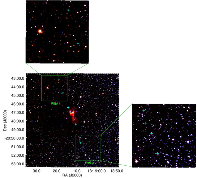
Figure 5. JHK color-composite image of the HH80-81 jet, with K-band emission shown in red, H-band emission in green and J-band in blue. Knots 1–9 are marked with cyan crosses. The green boxes marked as Fields 1 and 2 show two regions toward the northern and southern arms of the jet, respectively.
Download figure:
Standard image High-resolution image