Abstract
Accurate forecasting of geomagnetic disturbances is essential for mitigating space weather effects on critical infrastructure. We present an optimized Long Short-term Memory neural network (LSTM+), refined through a reforecast procedure and hyperparameter tuning using data from Solar Cycle 24, achieving high predictive skill. For Solar Cycle 24, the model demonstrates a Nash–Sutcliffe efficiency of 0.95 for Ap and 0.78 for Dst, with Pearson correlation coefficients of 0.983 and 0.901, respectively. Furthermore, the error rate for predicting the peak Ap and trough Dst values was low, at 4.16% and 7.77%, respectively. This LSTM+ model is used to predict the Ap and Dst indices for Solar Cycle 25. The model forecasts a peak in Ap around 2026 January and a trough in Dst around 2026 February, consistent with the observed lag of up to 3 yr between geomagnetic indices and the sunspot number maximum in prior cycles. Validation against historical data confirms the model’s reliability in capturing these temporal offsets. These projections offer a predictive framework for improving space weather preparedness and safeguarding technological systems.
Original content from this work may be used under the terms of the Creative Commons Attribution 4.0 licence. Any further distribution of this work must maintain attribution to the author(s) and the title of the work, journal citation and DOI.
1. Introduction
Solar activity continuously influences Earth’s magnetosphere, driving geomagnetic disturbances. While coronal mass ejections (CMEs) are indeed more frequent during periods of high solar activity, characterized by increased sunspot numbers (SSNs) and solar flares, corotating interaction regions (CIRs) are typically more prevalent during the declining phase and solar minimum of the solar cycle. Both CMEs and CIRs originate from the Sun and can generate geomagnetic storms through different mechanisms (M. G. Kivelson & C. T. Russell 1995; I. G. Richardson & H. V. Cane 2012). These disturbances are amplified during periods of high-level solar activity, characterized by increased SSNs, solar flares, and the more frequent occurrence of CMEs and CIRs. The impacts of geomagnetic disturbances on critical infrastructure, as detailed by C. J. Schrijver et al. (2015), extend from power grid disruptions caused by geomagnetically induced currents to increased radiation risks for satellites, aircraft, and even personnel. While short-term forecasts address immediate threats, their work implicitly supports the need for long-term probabilistic forecasting. Such forecasts provide the crucial lead time necessary for sectors like power utilities and airlines to implement proactive mitigation strategies, optimizing maintenance, operations, and infrastructure investments to enhance long-term resilience.
Geomagnetic activity is typically characterized by a variety of indices, each reflecting different aspects of the Earth’s magnetic field variations. This study focuses on two key indices, Ap and Dst, due to their established relevance in space weather applications. Ap, derived from the planetary Kp index (J. Bartels 1949), provides a global measure of geomagnetic activity at mid-latitudes, capturing both minor and major disturbances. This index is particularly valuable for assessing potential disruptions to radio communications and navigation systems, which are sensitive to ionospheric variations driven by geomagnetic activity. Dst, on the other hand, quantifies the intensity of the symmetric ring current encircling the Earth (M. Sugiura & K. Kamei 1991). Negative Dst values indicate a strengthening of the ring current, typically associated with geomagnetic storms, with more negative values signifying more intense storms (M. Nose et al. 2015). Dst is a critical parameter for assessing potential impacts on satellite operations, power grids, and pipelines, which are vulnerable to the enhanced particle fluxes and magnetic field variations associated with geomagnetic storms. The choice of Ap and Dst allows for a comprehensive assessment of geomagnetic activity and its potential consequences for a range of technological systems.
Recent studies have investigated the use of deep learning and data assimilation techniques to enhance Dst forecasting accuracy. For instance, J. Zhang et al. (2023) evaluated the performance of Long Short-term Memory (LSTM) and Empirical Mode Decomposition–Long Short-term Memory (EMD-LSTM) models for Dst index prediction. They revealed that while LSTM achieved marginally higher overall accuracy, EMD-LSTM demonstrated superior performance in reducing prediction lag and forecasting geomagnetic storms. This highlights the distinct strengths of each model, suggesting nuanced application depending on forecasting priorities. B. Nilam & S. T. Ram (2022) demonstrated the high accuracy of the ensemble Kalman filter (EnKF) for Dst forecasting, particularly during severe geomagnetic storms, through the assimilation of real-time data. Significantly, Y. Abduallah et al. (2022) introduced the Dst Transformer, a novel Bayesian deep learning model that surpasses existing methods in both accuracy and uncertainty quantification for Dst forecasting. This study represents the first application of a Bayesian deep learning approach specifically designed for predicting the Dst index.
Accurate forecasting of the Ap index remains a significant challenge. E. Paouris et al. (2021) performed a detailed statistical evaluation of current predictive methods, showing that models achieve limited success, with correlation coefficients ranging from 0.6 to 0.8 and notable errors in high-activity periods. Their work highlights the need for integrating advanced models and leveraging precise solar data to improve predictive reliability. R. L. McPherron (1999) used linear prediction filters, specifically autoregressive moving average models, that incorporate past Ap index behavior and solar wind velocity as inputs, demonstrating the capability to predict up to 57% of the variance in the Ap index and, in some cases, surpassing human forecasters in performance. These findings highlight the need for exploring advanced techniques, like incorporating solar wind parameters, to enhance Ap index forecasting accuracy, particularly for longer lead times.
In this work, the optimized LSTM+ model is trained on the historical values of Dst and Ap to forecast their future variations during Solar Cycle (SC) 25. The predicted results are compared with the identified relationships from previous cycles to determine the periods during which the indices are expected to reach their minimum or maximum values. This investigation is anticipated to facilitate the enhancement of predictive frameworks for geomagnetic activity and to augment our insights into the forecasting of space weather phenomena.
2. Data Sources
Data pertaining to the Dst and Ap index were retrieved from the OMNIWeb Plus data set, curated by NASA’s Space Physics Data Facility (SPDF) and available at https://spdf.gsfc.nasa.gov/pub/data/omni/low_res_omni/, (omni_yearly.dat and omni_27 av.dat). To investigate geomagnetic variations throughout SC25 using the LSTM+ model, 27 day averages were employed. Missing values in the 27 day averaged OMNI data were addressed using cubic spline interpolation, a method that ensures smooth and continuous time series by fitting cubic polynomials to the existing data. To mitigate the inherent noise in the data and facilitate accurate identification of minima, maxima, and their corresponding times, we applied a Gaussian smoothing filter. This filter effectively attenuates high-frequency variations while preserving the underlying trends relevant to solar cycle analysis (D. H. Hathaway et al. 1999). As demonstrated by D. H. Hathaway (2015) and commonly employed by space weather agencies like NOAA/SWPC in their solar cycle progression monitoring,3 data smoothing is a standard technique for analyzing solar activity data. The Gaussian-shaped filter is applied to smooth the input data, enabling us to reveal long-term trends and cyclical patterns that might be obscured by short-term fluctuations.
The weight function of the Gaussian filter, as described by D. H. Hathaway (2015), is given by

where t represents the time lag in months relative to the central data point, ranging from −2a + 1 to +2a − 1. The parameter 2a is defined as the full width at half-maximum (FWHM) of the filter, which in our case is set to 24 months to smooth variations within approximately a 2 yr timescale, consistent with typical solar cycle analysis practices (D. H. Hathaway 2015). A larger FWHM results in a wider filter and thus stronger smoothing, effectively controlling the degree of high-frequency noise reduction. The filtered (smoothed) output data point at a given time is calculated as a weighted average of the unsmoothed input data points within the filter window, with weights determined by the Gaussian function. This process emphasizes data points closer to the central time, while progressively downweighting points further away, effectively isolating the underlying long-term signal.
While Gaussian smoothing inherently introduces a degree of data leakage by using future data points, this is a recognized trade-off. For our focus on solar cycle analysis and long-term trend extraction, Gaussian smoothing is intentionally employed to reveal underlying cyclical patterns by removing high-frequency noise. In this context of retrospective analysis, the benefits of enhanced signal clarity for understanding long-term dynamics outweigh the limitations of minor data leakage, making it a well-established technique for our analytical purposes.
3. Prediction Procedure
3.1. The LSTM+ Model
To forecast geomagnetic activity, this study employs the LSTM+ model, which is based on the standard LSTM network architecture but incorporates a crucial optimization, named as the reforecast procedure. While standard LSTM networks inherently process sequential data by passing the hidden state from one time step to the next, in the LSTM+ model, we introduce an iterative feedback mechanism that leverages the model’s own predictions to enhance its forecasting capability for extended horizons. A more detailed description of the LSTM+ architecture, including its enhancements over traditional LSTM networks and its application to solar activity forecasting, can be found in H. Zhu et al. (2022, 2023).
In a traditional LSTM, for a given input sequence xt−n,…, xt, the model predicts a sequence ht+1,…, ht+m. The internal LSTM cell naturally propagates information through hidden states. However, in the standard approach, to generate predictions for multiple future time steps (m > 1), the model typically relies solely on the initial input and its learned internal dynamics to extrapolate into the future. The LSTM+ model deviates from this standard approach through its reforecast procedure, visually depicted in Figure 1. Instead of relying solely on historical data for each prediction step within the forecast horizon, the reforecast procedure iteratively feeds the most recent forecasted output back into the model as input for subsequent predictions.
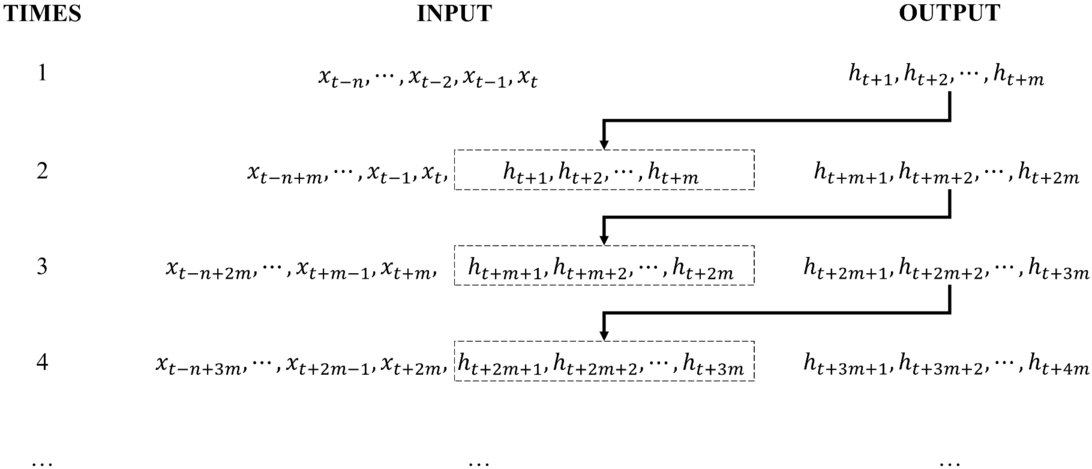
Figure 1. Workflow of the reforecast procedure in LSTM+ model. This figure illustrates the iterative prediction process. At each time step, the model takes an input sequence and generates a forecast. This forecast then becomes part of the input for the next prediction step, creating a chain of forecasts.
Download figure:
Standard image High-resolution imageThis iterative refeeding of forecast outputs creates a chain of predictions, where each subsequent forecast is conditioned not only on historical data but also on the model’s own prior forecasts. This dynamic approach allows the LSTM+ model to adapt to evolving patterns and potentially capture genuine time series trends more effectively than traditional LSTM models that solely rely on historical data for extended forecasts.
3.2. Performance Indices
This study focuses on forecasting Ap and Dst trends during SC25, with a particular emphasis on accurately predicting the timing of peak activity. To rigorously evaluate the performance of the LSTM+ model, we employed four metrics. The Nash–Sutcliffe efficiency coefficient (NSE) quantifies the model’s predictive skill compared to a baseline forecast using the mean of the observed data. NSE ranges from negative infinity to 1. An NSE of 1 indicates that the model predictions perfectly match the observations in terms of variance explained by the model relative to the variance of the observations themselves. It signifies a perfect model fit according to the NSE metric, not necessarily a flawless real-world prediction in every aspect. An NSE of 0 indicates performance equivalent to the mean of the observed data. The absolute percentage error ( ) was used to assess the accuracy of the predicted peak/trough values, while the absolute time difference (
 ), in days, between predicted and observed times, evaluated the accuracy of the timing. In addition, the Pearson correlation coefficient (
 ) measured the linear agreement between predicted and observed trends. The mathematical definitions of these metrics are provided below.
  denotes the peak value of the actual value, and
  denotes the peak value of the predicted value. And
  represents the
  actual value, and
  represents the
  predicted value.
  is the average of the actual values, and
  is the average of the predicted values.
  and
and  represent the actual and predicted time value of the peak value in days, respectively.




3.3. Data Preprocessing and Model Validation
To prepare the data for LSTM+ model training and evaluation, we employed a cycle-specific normalization technique. The 27 day averaged Ap and Dst index data, spanning SC21–SC24, were individually normalized within each solar cycle to a mean of 0 and a standard deviation of 1. This preprocessing step was crucial to mitigate the inherent variability in the intensity of different solar cycles, allowing the model to focus on learning the underlying temporal patterns and cyclical dynamics of geomagnetic activity, rather than being biased by absolute magnitude differences across cycles. For model development and internal validation, we partitioned the SC21–SC23 data into training and validation sets using a 70%–30% split. The first 70% of the SC21–SC23 data was designated for training, while the remaining served as an internal test data set during the training process.
To rigorously evaluate the out-of-sample predictive capabilities of the trained LSTM+ model on truly unseen data, we conducted a separate evaluation against the actual observed Ap and Dst values for SC24. While the actual observed values of SC24 were not utilized during the neural network weight training, the predictive performance on SC24 was subsequently employed as the primary criterion for evaluating and selecting the optimal hyperparameter configurations in our optimization procedure. For this out-of-sample evaluation, we fed the LSTM+ model with historical data from the latter portion of SC23 as input, and then compared the resulting multi-step predictions against the corresponding actual Ap and Dst values from SC24. The performance metrics reported in Table 1 and visualized in Figure 2 are based on this rigorous out-of-sample evaluation against SC24 data, providing a robust assessment of the model’s generalization ability to forecast geomagnetic activity in a truly predictive setting.
Table 1. The Results of Four Evaluation Indices for the Prediction of SC24 in the LSTM+ Model and Other Compared Models.

|

|

|

| ||
|---|---|---|---|---|---|
| (%) | (days) | ||||
| Ap(peak) | LSTM+ | 0.95 | 4.16 | −27 | 0.983a |
| Linear | 0.00 | 99.59 | 1485 | 0.375a | |
| Average | 0.81 | 10.31 | −189 | 0.899a | |
| ARIMA | 0.26 | 92.27 | −729 | 0.660a | |
| BP | −4.07 | 61.32 | −1431 | −0.458a | |
| DST(trough) | LSTM+ | 0.78 | 7.77 | 189 | 0.901a |
| Linear | −0.06 | 106.74 | −2430 | −0.082 | |
| Average | 0.60 | 23.92 | −324 | 0.784a | |
| ARIMA | −5.55 | 202.14 | −1647 | 0.408a | |
| BP | −0.35 | 3.13 | −540 | 0.45a | |
Note.
aCorrelation is significant at the 0.01 level (two-tailed).Download table as: ASCIITypeset image
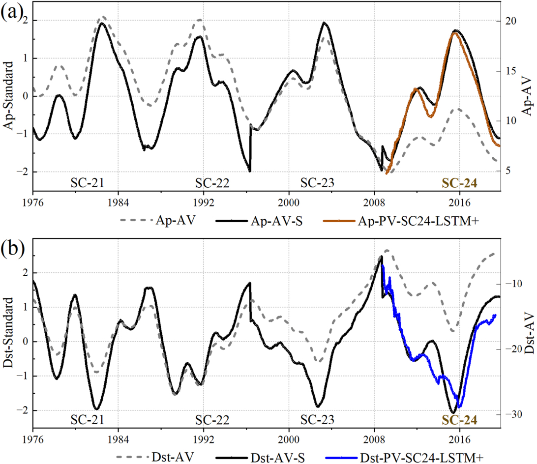
Figure 2. Observed and Predicted Ap and Dst Values from SC21 to SC24. (a) Shows unnormalized observed Ap (gray dashed), normalized observed Ap (black solid), and normalized prediction for SC24 (brownish-yellow). (b) Shows unnormalized observed Dst (gray dashed), normalized observed Dst (black solid), and normalized prediction for SC24 (blue).
Download figure:
Standard image High-resolution imageThe LSTM+ model, implemented using TensorFlow/Keras, employed a straightforward yet effective architecture consisting of a single LSTM layer followed by a Dense output layer. The LSTM layer’s capacity, controlled by the number of neurons, was systematically explored during hyperparameter optimization, ranging from 10 to 100 neurons in increments of 5. The input sequence length, representing the historical data window, was explored from 10 to 100 in steps of 1. The output layer was configured with a neuron count matching the prediction horizon, which was optimized at values of 6 and 12. Model training was performed using the Adam and Nadam optimizer, respectively, with their default learning rate and the mean absolute error loss function. The batch size was set to 100 based on prior experience. The number of training epochs, also determined through manual optimization, was varied across values of 100, 200, 300, 400, and 500 epochs. Hyperparameter selection was guided by monitoring validation loss on an internal validation set (derived from a split of the SC21–SC23 training data) and evaluating performance metrics on the out-of-sample SC24 test data set. Early stopping was not implemented, and a fixed random seed according to the length of SC24 was employed across all experiments to ensure reproducibility of the results.
To provide a comprehensive evaluation of the LSTM+ model’s predictive capabilities for SC24, its performance was benchmarked against several baseline models, including a simple linear regression model (linear), a historical cycle average model (average), an Autoregressive Integrated Moving Average (ARIMA) model, and a standard backpropagation (BP) neural network. The comparative results for Ap and Dst indices, based on the NSE,  ,
,  , and r, are presented in Table 1. The LSTM+ model consistently demonstrates superior predictive skill for SC24 across both Ap and Dst indices. For Ap, the LSTM+ model achieves a high NSE of 0.95, a low
  of 4.16% for the peak value (with a timing difference
  of −27 days), and a strong Pearson correlation (r = 0.983, p < 0.01). Similarly, for Dst, the LSTM+ model yields an NSE of 0.78, an
  of 7.77% for the trough value (
 = 189 days), and a robust correlation (r = 0.901, p < 0.01).
In contrast, the baseline models exhibited considerably weaker performance. The linear regression model struggled to capture the cyclical nature of the indices, resulting in NSE values near or below zero (0.00 for Ap, −0.06 for Dst) and very large errors in peak/trough prediction. The ARIMA model via automated order selection showed modest improvement for Ap (NSE = 0.26, r = 0.660) but performed poorly for Dst (NSE = −5.55), with substantial errors in predicting the extrema for both indices. The BP neural network, a simpler feedforward architecture, also underperformed relative to LSTM+, yielding negative NSE values for Ap (−4.07) and Dst (−0.35), although it achieved a notably low  for the Dst trough (3.13%), its overall predictive accuracy and timing were poor. Interestingly, the historical average model, which predicts SC24 based on the resampled average of standardized SC21–23, demonstrated respectable performance, particularly for Ap (NSE = 0.81, r = 0.899) and Dst (NSE = 0.60, r = 0.784). This suggests that an average cyclical pattern contains significant predictive information. However, the LSTM+ model still surpassed the average model across all metrics, especially in achieving lower
  and more accurate
  for Ap, and higher NSE and r for Dst.
These comparative results underscore the advanced capabilities of the LSTM+ architecture. Its ability to learn complex temporal dependencies and nonlinear dynamics allows it to significantly outperform simpler statistical methods, basic neural networks, and even a historical averaging approach in the challenging task of long-term geomagnetic index forecasting. The superior NSE and correlation values, coupled with more accurate peak/trough predictions, affirm the LSTM+ model’s robustness and its suitability for forecasting solar-cycle-scale geomagnetic activity.
Figure 2 displays the observed and LSTM+ model-predicted Ap and Dst indices, including the original data and normalized to a mean of 0 and a standard deviation of 1 within each solar cycle. Observed original values (in gray dashed lines) and normalized values (in black solid lines) are shown for SC21–SC24. Model predictions are shown for SC24 only, with Ap predictions in brownish-yellow and Dst predictions in blue. The LSTM+ model effectively captures the overall trends and magnitudes of both Ap and Dst during SC24. For Ap, the predicted peak closely aligns with the observed peak, although slightly preceding it. The model also accurately reproduces the broader variations in Ap throughout the cycle. For Dst, the model successfully predicts the timing and depth of the minimum value, as well as the general trend, though with some deviations during the rising phase of the cycle.
4. Results and Discussion
For the prediction of SC25, the model utilized the parameter combination in the LSTM+ model that demonstrated the most favorable predictive performance, which we defined based on a two-pronged evaluation approach. This “most favorable performance” was determined by jointly considering: (1) the LSTM+‘s forecasting accuracy for SC24, assessed across all evaluation indices as detailed in Section 3.2, and (2) a comparison of vision and relevance of the SC25 predictions generated using these parameters against the available actual values for SC25. The parameter combination that yielded the best balance of high evaluation metrics for SC24 and visually plausible and consistent predictions with a high correlation coefficient for the initial portion of SC25 was selected as representing the “most favorable performance.” The predicted results of the Ap and Dst in SC25 were also presented in normalized form (a mean of 0 and a standard deviation of 1 within SC25). The decision to perform this independent normalization stemmed from the research objective, which prioritizes characterizing the temporal evolution of Ap and Dst within SC25, rather than making direct comparisons of absolute intensities across cycles. Therefore, normalization was conducted outside the LSTM+ model framework to ensure that the model’s predictions remained focused on capturing the time-dependent trends and cyclical structure inherent in the Ap and Dst data, facilitating a more accurate and nuanced forecast for SC25.
Figure 3 illustrates the temporal evolution of Ap and Dst, throughout SC25. The figures present a comparative analysis of the observed smoothed values (denoted as Ap-AV and Dst-AV) and the predicted values generated by the LSTM+ model (denoted as Ap-PV and Dst-PV). Statistical analysis reveals a robust positive correlation between the observed and predicted values for both indices. Pearson correlation coefficients both reach 0.978 for Ap and Dst, with statistically significant (p < 0.05). This strong correlation underscores the model’s capacity to accurately capture the underlying temporal patterns and trends of these geomagnetic indices. Furthermore, the LSTM+ model identifies the timing of the Ap maximum and the Dst minimum, projected to occur in 2026 January and February, respectively. To assess the temporal relationship between peak Ap and minimum Dst values, we analyzed smoothed data from SC21 through SC24. In cycles 21, 23, and 24, the Ap maximum occurred 162, 216, and 81 days after the Dst minimum, respectively. SC22 presented a more complex pattern with two similar Dst minima. The Ap maximum in cycle 22 occurred just 27 days after the second Dst minimum.
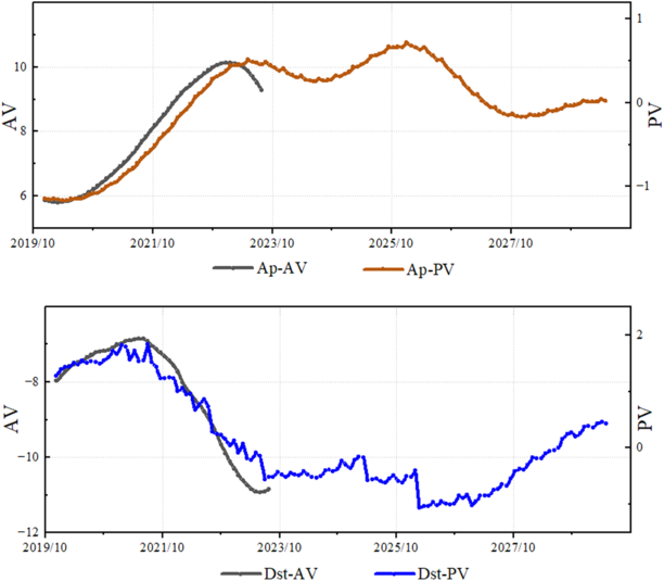
Figure 3. Comparison of the actual values of AV (Ap-AV) and Dst (Dst-AV) in SC-25 the predicted values (Ap-PV and Dst-PV) obtained from the LSTM+ Model, respectively.
Download figure:
Standard image High-resolution imageWhile the smoothing process inherently introduces some uncertainty in pinpointing the precise timing of these extrema, the general trend suggests a temporal coincidence between the peak of the Ap index and the minimum of the Dst index within each solar cycle. This temporal relationship can be physically understood by considering the distinct solar drivers influencing geomagnetic activity throughout the solar cycle. Both Ap and Dst indices reflect solar-driven disturbances, yet they exhibit differential sensitivities to various aspects of these phenomena. The Dst index, a measure of geomagnetic storm intensity, typically reaches its most negative values, indicative of strongest storms, during periods of heightened solar activity, often around the solar cycle maximum. Conversely, the Ap index, which quantifies the overall level of global geomagnetic activity, responds to a broader spectrum of disturbances. This includes not only the intense, transient events characteristic of solar maximum, but also more sustained, longer-duration solar wind structures that become increasingly prominent during the declining phase of the solar cycle. Consequently, while the most pronounced Dst minima, associated with major geomagnetic storms, are frequently observed near solar maximum, the comprehensive level of geomagnetic activity, as reflected by Ap, can remain elevated and may even peak slightly later in the cycle. This temporal overlap in the occurrence of diverse geomagnetic disturbances, each contributing uniquely to Ap and Dst, plausibly accounts for the generally observed coincidence between the Ap maximum and Dst minimum within each solar cycle.
Analysis of past annual mean data for Ap, Dst, and SSNs reveals a consistent tendency that the AP peak typically coincides with the Dst trough, both lagging behind the SSN peak by 1 to 3 yr, which is consistent with the observation of others (O. S. Oyekola 2018). Preliminary observations indicate that the unsmoothed monthly average SSN for SC25 reached its maximum in 2024 July. While further data is needed for confirmation, this potentially represents the ultimate peak for the current solar cycle. Notably, our model’s prediction of an Ap peak and Dst trough in the beginning of 2026 falls within 1 to 3 yr of this observed SSN peak, well within the established historical lag range.
5. Conclusions
The geomagnetic disturbances in SC25 were forecasted with the optimized LSTM+ model, which included a novel reforecasting procedure, and demonstrated exceptional predictive performance. Trained and validated using data from SC21 through 23, the model accurately predicted the peak Ap value and the though Dst value for SC24, achieving high Nash–Sutcliffe efficiency coefficients (0.95 and 0.78, p < 0.05) and strong Pearson correlation coefficients (0.983 and 0.901, p < 0.05), respectively. Then, according to the optimized parameters of the LSTM+ model based on SC24 performance, we forecasted the temporal evolution of Ap and Dst throughout SC25. The model’s predictions, normalized within SC25 to emphasize intracycle dynamics, exhibited a strong positive correlation with observed smoothed Ap and Dst values (Pearson correlation coefficient of 0.978 for both, p < 0.05).
The model projects the Ap maximum and Dst minimum to occur in 2026 January and February, respectively. Analysis of SC21–SC24 reveals that Ap maxima and Dst minima generally occur within the same year. However, variations in precise timing and the occurrence of multiple Dst minima in certain cycles introduce complexity. The predicted timing of the Ap peak and Dst trough in early 2026 aligns with the observed historical lag of 1 to 3 yr following the SSN peak, which preliminarily appears to have occurred in 2024 July. While these results provide valuable insights into the expected geomagnetic activity during SC25, continued monitoring and analysis of solar and geomagnetic data are essential for validating these predictions and further refining our understanding of the Sun–Earth connection.
Acknowledgments
This research was supported by the Start-Up Fund for new Ph.D. Researchers of Suzhou Chien-Shiung Institute of Technology. We acknowledge the use of Ap and Dst data from NASA’s Space Physics Data Facility (SPDF), USA (https://spdf.gsfc.nasa.gov/pub/data/omni/low_res_omni/). Sunspot data from the World Data Center SILSO, Royal Observatory of Belgium, Brussels (F. Clette & L. Lefèvre 2015).