Abstract
Current state-of-the-art spectrographs cannot resolve the fundamental spatial (subarcseconds) and temporal (less than a few tens of seconds) scales of the coronal dynamics of solar flares and eruptive phenomena. The highest-resolution coronal data to date are based on imaging, which is blind to many of the processes that drive coronal energetics and dynamics. As shown by the Interface Region Imaging Spectrograph for the low solar atmosphere, we need high-resolution spectroscopic measurements with simultaneous imaging to understand the dominant processes. In this paper: (1) we introduce the Multi-slit Solar Explorer (MUSE), a spaceborne observatory to fill this observational gap by providing high-cadence (<20 s), subarcsecond-resolution spectroscopic rasters over an active region size of the solar transition region and corona; (2) using advanced numerical models, we demonstrate the unique diagnostic capabilities of MUSE for exploring solar coronal dynamics and for constraining and discriminating models of solar flares and eruptions; (3) we discuss the key contributions MUSE would make in addressing the science objectives of the Next Generation Solar Physics Mission (NGSPM), and how MUSE, the high-throughput Extreme Ultraviolet Solar Telescope, and the Daniel K Inouye Solar Telescope (and other ground-based observatories) can operate as a distributed implementation of the NGSPM. This is a companion paper to De Pontieu et al., which focuses on investigating coronal heating with MUSE.
Original content from this work may be used under the terms of the Creative Commons Attribution 4.0 licence. Any further distribution of this work must maintain attribution to the author(s) and the title of the work, journal citation and DOI.
1. Introduction
We live in the Sun's extended atmosphere, which is continually shaped by its changing magnetic landscape. The quiescent state of the Sun and its wind is punctuated by flares (Fletcher 2005; Zharkova et al. 2011; Toriumi & Wang 2019b), coronal mass ejections (CMEs, Forbes & Priest 1995), and solar energetic particle (SEP) events (Klein & Dalla 2017). While solar progenitors of space weather effects are recognized to pose a threat to our technological civilization, our ability to predict their occurrence and impact is hampered by an incomplete picture of underlying physical drivers, triggers, and instabilities.
Providing narrowband extreme ultraviolet (EUV) images at 12 s cadence, the Atmospheric Imaging Assembly (AIA; Lemen et al. 2012) on board NASA’s Solar Dynamics Observatory (SDO; Pesnell et al. 2012) has demonstrated the importance of high temporal cadence in order to “freeze” coronal dynamics, especially during eruptive events. Two shortcomings of SDO/AIA are its spatial resolution (∼1″) and the lack of spectroscopic information necessary to understand the 3D flow fields in solar eruptive events. As demonstrated by the Hinode/Solar Optical Telescope (SOT; Hinode Review Team et al. 2019) and ground-based observatories (GBOs; e.g., Scullion et al. 2014; Jess et al. 2015; Jing et al. 2016; Wang et al. 2018; Yadav et al. 2021) for the solar photosphere and by the Interface Region Imaging Spectrograph (IRIS) for the chromosphere and transition region (see De Pontieu et al. 2021, and references therein), there is a plethora of subarcsecond structures in flaring and eruptive regions. Targeted for launch in 2026, the High Throughput EUV Solar Telescope (EUVST) is a single-slit spectrograph with subarcsecond spatial resolution and complete temperature coverage from the chromosphere (20,000 K) to the flaring corona (20 MK; see Shimizu et al. 2020). Since EUVST does not have context imaging in coronal lines, its operation would benefit from coordinated observations by other instruments with subarcsecond imaging capability.
Our observational capacity to probe small-scale dynamic processes in the lower atmosphere will be enhanced as the Daniel K. Inouye Solar Telescope (DKIST; Rimmele et al. 2020; Rast et al. 2021) begins operations. We do not currently have regular subarcsecond coronal observations. Short observational campaigns lasting several minutes by the sounding rocket mission Hi-C (Cirtain et al. 2013; Rachmeler et al. 2019; Tiwari et al. 2019) and by the Extreme Ultraviolet Imager (EUI; Berghmans et al. 2021) on board the Solar Orbiter mission (Müller et al. 2020) have demonstrated the discovery potential of subarcsecond resolutions. However, their chances of capturing solar eruptive events are hampered by the short suborbital flight time and deep-space telemetry restrictions, respectively. In addition, for the Solar Orbiter, the restricted time interval of perihelion passage further reduces the chances of catching a flare/CME at the highest spatial resolution. Furthermore, like SDO/AIA, these instruments provide narrowband imaging and lack spectroscopic information for measuring Doppler flows and nonthermal broadening of the targeted emission lines.
Although primarily designed for studying the chromosphere and transition region, IRIS has also provided important spectral diagnostics of the flaring corona. Thanks to its subarcsecond spatial resolution, IRIS has provided a new view of several aspects of flares (see De Pontieu et al. 2021, for a review), ranging from finally resolving chromospheric evaporation sites (fully blueshifted Fe xxi 1354 Å line profiles; e.g., Brosius & Daw 2015; Graham & Cauzzi 2015; Li et al. 2015; Polito et al. 2015; Tian et al. 2015; Young et al. 2015; Tian & Chen 2018)—solving a long-standing problem (e.g., Doschek et al. 1986; Young et al. 2013)—to observing Fe xxi redshifts above the flare loop top (Tian et al. 2014), which are a possible signature of downward-moving reconnection outflows or hot retracting loops, predicted by flare models. However, with a single-slit spectrograph design, IRIS has only allowed us a peek into the full richness of the waves and nonlinear instabilities that pervade the solar corona. Without near-simultaneous spectral coverage of active region (AR)-scale fields of view (FOV), we will continue to be blindsided, unable to resolve fundamental questions about solar coronal activity. As this paper demonstrates, spectroscopic observables at subarcsecond resolution and at cadences of <20 s are crucial for understanding solar flaring and eruptive activity, including distinguishing physical triggers of eruptions, characterizing intermittency and turbulent structures in current sheets and reconnection outflows, and constraining the initial conditions of CMEs.
This paper is structured as follows. In Section 2, we introduce the Multislit Solar Explorer (MUSE; Cheung et al. 2019; De Pontieu et al. 2020), a mission undergoing a Phase A study as a NASA Heliophysics Medium-class Explorer, which will fill the aforementioned observational gap. In Section 3, we discuss the central role of advanced numerical modeling to the MUSE science investigation. In Section 4, we discuss the background and science objectives of the Next Generation Solar Physics Mission (NGSPM; Scientific Objectives 2017) and suggest how MUSE, EUVST, and DKIST (and other GBOs) can coordinate as a distributed implementation of the NGSPM. In Section 5, we use numerical models to demonstrate how MUSE is unique in its capability for exploring the solar coronal dynamics and for constraining models of solar flares and eruptions. A companion paper (De Pontieu et al. 2022) serves similar purposes but in the context of the coronal heating problem.
2. The MUSE Observatory and Science Investigation
Currently undergoing Phase A study as a NASA Heliophysics Medium-class Explorer mission, MUSE has the following science goals:
- 1.Determine which mechanism(s) heat the corona and drive the solar wind.
- 2.Understand the origin and evolution of the unstable solar atmosphere.
- 3.Investigate fundamental physical plasma processes.
MUSE’s 37-slit EUV spectrograph (SG) operating at three wavelength bands (108, 171, and 284 Å), offers AR-scale (FOV of 170″ × 170″) spectral rasters at 0167 along the slits and at 0
4 spatial sampling across the slits, all at a cadence as fast as of 12 s (see Figure 1). Each parallel slit (along the detector Y-direction) produces its own 2D spectral image on the detector, but they offset from each other on the detector in the x-direction. By choosing narrow bandpasses to target isolated spectral lines (Fe ix 171 Å at 0.7 MK, Fe xv 284 Å at 2 MK, Fe xix at 108 Å at 10 MK, and Fe xxi 108 Å at 12 MK; see Figure 1), optimizing for the interslit spacing and by using a compressed sensing method, it has been shown that the detector signal can be processed to retrieve physical observables (e.g., emission measure, Doppler velocity) simultaneously sampled by the 37 slits (Cheung et al. 2019; De Pontieu et al. 2020).
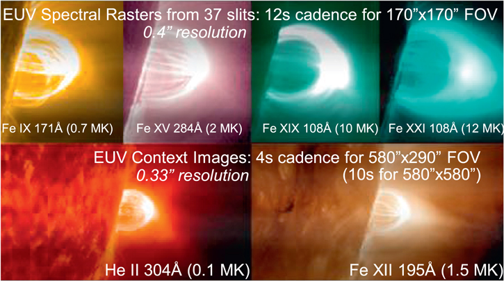
Figure 1. FOVs and cadences of MUSE’s multislit SG and Context Imager (CI).
Download figure:
Standard image High-resolution imageThis revolutionary multislit design allows MUSE to capture AR-scale rasters at 30×–100× the speed of existing or planned EUV spectrographs (e.g., Solar & Heliospheric Observatory/Solar Ultraviolet Measurements of Emitted Radiation, Hinode/EUV Imaging Spectrometer (EIS), and the upcoming EUVST). This capability allows MUSE to effectively capture the coronal/transition region (TR) dynamics while delivering valuable spectroscopic information about the fundamental physical processes. In addition to the SG, the CI provides 033 resolution narrowband images in an even larger FOV (580″ × 290″) in the 304 and 195 Å bands (4 s cadence single channel, 8 s cadence dual channel).
3. Numerical Simulations
A major component of the MUSE investigation is the use of state-of-the-art numerical models, which are key to addressing MUSE’s science goals, to demonstrate the need for high-cadence and high-resolution imaging spectroscopy, and to illustrate how MUSE observables will test current theory, and improve existing models. Such forward modeling exercises tell us how MUSE can discriminate between models and physical mechanisms. Models used by the team to study the diagnostic potential of MUSE in the context of flares and eruptions are listed in Table 1. They include 1D field-aligned radiation hydrodynamics (RHD), and 2D and 3D magnetohydrodynamics (MHD) models. For numerical models targeting the coronal heating question, refer to the companion paper (De Pontieu et al. 2022). For further descriptions of the models, refer to Appendix A. For a discussion of how synthetic observables are computed, the reader should consult Appendices B and C.
Table 1. Numerical Simulations Used to Synthesize MUSE Observables
| Code | Model | Target | Properties | NGSPM SO | References a |
|---|---|---|---|---|---|
| MURaM | MURaM_flare b | AR, flares, eruption | 3D MHD | II.1, II.2 | [1] |
| MURaM_circ_rib | Circular ribbon flares, eruption | 3D MHD | II.1, II.2 | [2] | |
| MURaM_collision | Colliding sunspots, eruption | 3D MHD | II.1, II.2, II.5 | [3] | |
| MURaM_emergence | Plage, flare | 3D MHD | II.1-II.2 | [4] | |
| Bifrost | B_npdns03 | Coronal hole, bright point, jets | 2D MHD | II.1, II.2, II.4 | [5] |
| ⋯ | Termination_shocks | Flare, magnetic reconnection | 2D MHD | II.4 | [6] |
| PREFT | Retracting_tube | Flare, magnetic reconnection | 1D MHD | II.4 | [7] |
| RADYN | RADYN_1D | Flaring loops and footpoints | 1D RHD, NTE | II.4 | [8,9] |
| RADYN_Arcade | Flaring loops (line-of-sight (LOS) effects) | 1D RHD, NTE + 3D AR loops | II.4 | [10] | |
Notes. RHD: radiative hydrodynamic; NTE: nonthermal electrons.
a References: (1) Cheung et al. (2019); (2) F. Chen et al. (2021, in preparation); (3) M. Rempel et al. (2021, in preparation), (4) Danilovic (2020); (5) D. Nóbrega-Siverio et al. (2021, in preparation); (6) Takasao et al. (2015); Takasao & Shibata (2016); (7) Longcope & Klimchuk (2015); Longcope et al. (2016); (8) Allred et al. (2015); (9) Polito et al. (2019); (10) Kerr et al. (2020b). b Publicly available at https://purl.stanford.edu/dv883vb9686.Download table as: ASCIITypeset image
As an example, consider Figure 2, which shows synthetic Fe xv 284 Å images computed from a radiative MHD simulation of an AR (MURaM_collision) in which two opposite polarity sunspots collide, eventually resulting in a flare and CME (see Figures 7 and 12 for the eruptive phase of the model). The top row of Figure 2 is the synthetic intensity image at the original simulation (horizontal) grid spacing of 192 km. The remaining rows show images degraded by (1) smoothing with a 2D Gaussian kernel of the form  (r is the distance from the origin in arcsec), followed by sampling onto a plate-scale with a pixel size of (Δx
, Δy
). The projected performance for MUSE/CI is σ = 0
(r is the distance from the origin in arcsec), followed by sampling onto a plate-scale with a pixel size of (Δx
, Δy
). The projected performance for MUSE/CI is σ = 014 (0
33 FWHM). For MUSE/SG, σ = 0
176 (0
4 FWHM). The CI has a pixel size of (Δx
, Δy
) = (0.143, 0.143)″. Note that the MUSE/CI has the Fe xii 195 Å and He ii 304 Å channels but does not include the Fe xv 284 Å channel. SDO/AIA lacks this channel. However, to illustrate the effect of instrumental resolution, we will use the same 284 Å line. For a MUSE dense SG raster with a step size of 0
4 and pixel size separation of 0
167 along the slit, (Δx
, Δy
) = (0.4, 0.167)″. To mimic the Gaussian core (due to charge spreading on the charge-coupled device) and the spatial sampling due to the plate-scales of SDO/AIA (Geostationary Operational Environmental Satellite, GOES/Solar Ultraviolet Imager, SUVI), we use σ = 0
49 (0
49) and Δx
= Δy
= 0
6(2
5).

Figure 2. High-resolution coronal observations by MUSE (033 for CI, 0
40 for the multislit SG), as well as the high sustained telemetry available will reveal small-scale structures (e.g., bright points and cross-loop striations) inaccessible to the current generation of solar instrumentation. These small-scale structures are important for constraining models of the coronal magnetic field and thermodynamic structure. The top row shows Fe xv 284 Å intensity images synthesized from the radiative MHD simulation MURaM_collision, which has a computational grid spacing of 192 km. The blue and red boxes indicate the FOVs of the magnified regions (left two columns). The remaining rows show the synthetic images degraded to the resolution and sampling of various instruments, including MUSE/CI, MUSE/SG, SDO/AIA, and GOES/SUVI.
Download figure:
Standard image High-resolution imageAs Figure 2 shows, subarcsecond-scale bright points and brightness striations across neighboring loops will be effectively captured by both MUSE/CI and MUSE/SG, but are lost at SDO/AIA and GOES/SUVI resolutions. This comparison illustrates only part of the benefits of MUSE. For each pixel position in the MUSE/SG raster, there will be spectroscopic information encoding the Doppler velocity and nonthermal broadening of coronal plasmas. In Section 5, we consider how such spectroscopic information at high cadence and spatial resolution can be exploited for MUSE’s science goals, as well as to address the NGSPM Science Objectives, which are detailed in the following section.
4. Next Generation Solar Physics Mission
The NGSPM (Scientific Objectives 2017) is a mission concept developed by a panel of solar physics experts designated by NASA, the Japan Aerospace Exploration Agency (JAXA), and the European Space Agency (ESA). 20 Following townhalls at international solar physics conferences and dozens of white-paper submissions from the community, the Science Objectives Team (SOT) developed a list of science objectives (SOs) based on the following criteria: (1) relevance to NASA/JAXA/ESA objectives, (2) scientific impact on solar physics, (3) scientific impact on other disciplines and research fields, (4) inability of current/planned missions and ground-based facilities to accomplish the objective, (5) need for space observations, (6) maturity of technology, (7) maturity of methodology, and (8) widespread interest within the solar physics community. Based on these factors, the NGSPM-prioritized SOs are as follows:
- 1.Formation mechanisms of the hot and dynamic outer solar atmosphere.
- 2.Mechanisms of large-scale solar eruptions and foundations for prediction.
- 3.Mechanisms driving the solar cycle and irradiance variation.
The companion paper De Pontieu et al. (2022) focuses on how MUSE and other observatories can coordinate to address NGSPM-I. This paper focuses on addressing NGSPM-II. Subobjectives of NGSPM-II are listed in Table 2.
Table 2. NGSPM Science Objectives a and Corresponding Mission Science Objectives
| NGSPM Science Objectives | Mission Science Objectives | ||
|---|---|---|---|
| MUSE b | EUVST c | DKIST d | |
| II. Mechanisms of large-scale solar eruptions | |||
| and foundations for prediction | |||
| II-1 Measure the energy buildup processes in flaring and CME regions | 2[a,b,d] | II-2-1 | 4.1, 5.6 |
| II-2 Identify the trigger mechanisms of solar flares and CMEs | 2[a,d],3 c | II-2-2 | 4.1,5.7 |
| and distinguish between the many CME models | |||
| II-3 Understand the evolution and propagation of CMEs and their effect | 2 c | ⋯ | 4.2 |
| on the surrounding corona | |||
| II-4 Understand the processes of fast magnetic reconnection | 3 c | II-1-[1,2,3] | 4.4, 5.3, 6.3 |
| II-5 Understand the formation mechanism of sunspots, | 1a,2b | II-[1,2]-1 | 3.4 |
| in particular delta sunspots | |||
Notes.
a https://hinode.nao.ac.jp/SOLAR-C/SOLAR-C/Documents/NGSPM_report_170731.pdf b De Pontieu et al. (2020). c https://hinode.nao.ac.jp/SOLAR-C/SOLAR-C/Documents/2_Concept_study_report_part_I.pdf d DKIST objective refers to section number in Rast et al. (2021).Download table as: ASCIITypeset image
The suite of instruments identified by the NGSPM report as the most suitable to address the prioritized SOs I and II are the following:
- 1.0
3 resolution coronal/TR spectrograph.
- 2.0
- 3.0
This combined observational capability may be implemented on a single platform (e.g., the original proposed Solar-C mission), or on multiple platforms. We argue the latter option can be fulfilled by appropriate coordination between MUSE and other observatories. The observational capability of (a) high-resolution coronal/TR spectrograph will be fulfilled by the high-throughput EUVST (Shimizu et al. 2020), which has been selected for implementation by JAXA and NASA, with a planned launch date in 2026. MUSE will serve as the high-resolution coronal/TR imager. It will not only provide context images continuously at very high cadence, but its multislit SG also provides spectroscopy, optimized to measure four spectral lines to facilitate high-cadence rasters.
As for (c), DKIST (currently in commissioning; Rimmele et al. 2020; Rast et al. 2021) and a number of other existing GBOs have already achieved or exceeded 01 resolution observations. They include the Swedish 1 m Solar Telescope (SST; Scharmer et al. 2003, 2019), GREGOR (Schmidt et al. 2012; Kleint et al. 2020), and the Goode Solar Telescope (previously, New Solar Telescope; Cao et al. 2010; Goode et al. 2010). In particular, SST observations have provided photospheric and chromospheric spectropolarimetric observation of flares at this spatial resolution (Yadav et al. 2021). The planned European Solar Telescope will add to this list of high-resolution GBOs for photospheric and chromospheric magnetometry. Coordination between DKIST and other GBOs with MUSE and EUVST can then be considered a distributed implementation of the NGSPM concept. Table 2 shows the correspondence of NSGPM SOs and the science goals/objectives of MUSE, EUVST, and DKIST.
5. Case Studies Addressing NGSPM Science Objective II
In the following, we present use cases of how MUSE observations will address questions regarding the drivers and triggers of solar flares and eruptions, how these events impact the ambient corona, and the underlying physical processes (such as fast magnetic reconnection). We will also highlight the synergies available through coordination with EUVST and with GBOs like DKIST. For this reason, the following sections are organized according to the subobjectives of NGSPM SO II.
5.1. II-1: Measure the Energy Buildup Processes in Flaring and CME Regions
Eruptive events originate in the solar atmosphere and are powered by the release of energy stored in stressed magnetic fields. The energy stored in the corona of flare- and CME-productive ARs is carried by flux emergence (Forbes & Priest 1995; Chen & Shibata 2000; Archontis & Hood 2008; Cheung & Isobe 2014; Toriumi & Wang 2019b), shearing/twisting (Amari et al. 2000; Wyper et al. 2017), perhaps driven by emergence of twisted fields (Manchester et al. 2004; Okamoto et al. 2010; Toriumi & Hotta 2019a), and cancellation of flux at polarity inversion lines (PILs) to form flux ropes (e.g., van Ballegooijen & Martens 1989; Cheung & DeRosa 2012; Savcheva et al. 2012; Kazachenko et al. 2014; Fisher et al. 2015; Chintzoglou et al. 2019). Measuring the energy buildup in flaring and CME regions can be done by modeling how the 3D magnetic field in the corona evolves (e.g., extrapolation methods; Wiegelmann & Sakurai 2012; DeRosa et al. 2015; Warren et al. 2018b), or by estimating the amount of energy deposited in the corona via the Poynting flux through the photosphere (see, e.g., Kazachenko et al. 2014). Both classes of methods rely on some combination of direct measurements of the field at the photosphere and chromosphere combined with measurements of field-aligned emission structures in the corona.
While photospheric vector magnetograms can be used as boundary conditions for nonlinear force-free field (NLFFF) extrapolations, because of the non-force-free nature of the photospheric field (due to confinement by ambient plasma pressure, for instance), systematic errors in the extrapolation may occur. To alleviate this problem, there are methods to reconstruct the coronal magnetic field using a combination of LOS (or radial component) magnetograms and EUV images of coronal loops (Aschwanden 2013; Malanushenko et al. 2014; Plowman 2021). Even when the reconstruction method does not directly use coronal imagery as input, the latter (e.g., by the locations of sigmoids and hot flux ropes) is needed for validation of the model (e.g., Savcheva et al. 2012; Wiegelmann & Sakurai 2012; James et al. 2018). As indicated in Figure 2, existing instruments, such as AIA and GOES/SUVI, do not have a sufficient spatial resolution to resolve small-scale loops (bright points) and cross-field striations between neighboring loops. Using loops traced at the coarse resolution available from existing instruments will lead to errors in the loop geometry, providing erroneous constraints on magnetic field reconstructions. Aschwanden et al. (2016) demonstrate how to use loops automatically traced in subarcsecond-resolution images in chromospheric images to complement loops traced in AIA images to constrain field extrapolations. With increased image contrast, MUSE images will increase the constraints (in terms of the number of traced loops and better loop geometries) for such field reconstruction approaches. This can have an impact on the estimates of the free magnetic energy available to power solar flares. EUVST can provide subarcsecond-resolution raster imaging, but to keep a high cadence (<20 s) rasters are limited to ∼5″ in width (see Figures 9 and 10). AR-scale rasters requires several minutes (assuming 1 s slit dwell time, 04 step sizes). Even at resolutions of 1″ or coarser, coronal loops evolve significantly over such timescales. This is especially true during the emerging phase of ARs. To provide observational constraints on the coronal magnetic field geometry, it is thus necessary to have both high-resolution and high-cadence imaging from MUSE.
Figure 3 shows MUSE Fe xv 284 Å maps synthesized from a flux emergence simulation (MURaM_emergence; see Table 1 and Appendix A). The spectroscopic rasters allows the retrieval of parameters such as total the line intensity as count rates of data number s−1 pix−1 (DN s−1 pix−1), as well as the Doppler shift and total line width (given here in units of km s−1). The line intensity (integrated over the wavelength), Doppler velocity, and line width maps all show strands with subarcsecond widths. The loop structures vary significantly in the span of tens of seconds, while an EUVST dense raster with 04 steps and slit dwell time of 1 s step−1 would require 100 s to complete a single raster. In comparison, the multislit design of the MUSE/SG allows for a dense raster to complete once every 12 s, and MUSE/CI will provide images in the 193 Å and 304 Å bands at 5 s cadence.
Figure 3. MUSE Fe xv 284 Å maps synthesized from a radiative MHD simulation of an emerging flux region (EFR; model MURaM_emergence, see Table 1 and Appendix A) reveals fine-scale coronal strands (subarcsecond widths) connecting opposite polarities of the emerging bipolar region, evolving on timescales of tens of seconds. MUSE rasters with 12 s cadence meets the requirements to track the dynamics of loops in EFRs. An animated version of this figure is available online, showing the evolution of the coronal loops over a duration of 620 s. The real-time duration of the animation is 2 s.
(An animation of this figure is available.)
Download figure:
Video Standard image High-resolution imageMUSE has a sufficiently large FOV to observe how nearby ARs interact (MUSE/SG FOV is 170″ × 170″). The CI extends the FOV to 580″ × 290″ (see Figure 1). This will enable studies of inter-AR interaction. Longcope et al. (2020) analyzed coronal loops in the AIA 171 Å channel in and around two ARs. They suggest that the coronal loops preferentially appear at the topological boundaries of magnetic subvolumes and that these are preferential sites for plasma heating (see also McCarthy et al. 2019). AIA and Hinode/EIS observations of transequatorial coronal loops connecting ARs located at positive and negative latitudes suggest there are observable characteristics particular to topological features such as separators (Ghosh & Tripathi 2020).
Coronal field configurations have topological features, which may leave imprints in spectroscopic observables. Synthetic maps of Fe xv emission, including line intensity, Doppler velocity, and line width as would be observed with MUSE, as shown in Figure 4, from a quiescent AR (preflare phase of model MURaM_collision), corroborate the suggestion by previous work that AR fan loop outflows are located at quasi-separatrix layers (QSLs). Baker et al. (2009) used Hinode/EIS rasters and coronal field extrapolations to show the fan loops have a different connectivity than the AR core loops. Therefore fan loop outflows (blueshifts and total line widths of tens of km s−1) are tracers of QSLs of AR boundaries. EUVST will be able to raster ARs in minutes (1 s slit dwell time, 04 raster steps), which would be sufficient for tracking slow changes in connectivity. However, the higher cadence of MUSE is needed to capture more dynamic changes, especially during flaring and eruptive scenarios.

Figure 4. Line intensity, Doppler velocity, and line width maps of the Fe xv 284 Å line synthesized from a radiative MHD model of a pair of sunspots approaching each other (MURaM_collision, see Table 1). The time stamp of this snapshot is relative to the time of the flare (see Figure 7 for the eruption flare phase), so this frame is in the quiescent phase when the coronal field is quasi-steadily adjusting in response to photospheric flows advecting two sunspots. The two spots are linked by S-shaped coronal loops in the line intensity image. At the periphery of the closed loop system are fan loops with Doppler blueshifts and line widths of tens of km s−1, signifying a change in connectivity.
Download figure:
Standard image High-resolution image5.2. II-2: Identify the Trigger Mechanism of Solar Flares and CMEs and Distinguish between the Many CME Models
Different CME models postulate reconnection in different places and at different times (see Patsourakos et al. 2020, for a review). For example, breakout models (Antiochos et al. 1999; Wyper et al. 2017) hypothesize reconnection above the flux rope, but tether-cutting models (Moore et al. 2001) say it is below. Longcope & Forbes (2014) developed a unified 2D model showing either mechanism (or a combination of both) can evolve a multipolar system with a preexisting flux rope to a loss of equilibrium, which explains CME acceleration as an ideal instability. In a series of 2.5D MHD experiments, (Karpen et al. 2012) demonstrated—for a system with azimuthal symmetry (and with a coronal flux rope that lacks anchored footpoints at the photosphere)—that breakout reconnection is the first to occur. In contrast, the torus instability (Kliem & Török 2006) does not require reconnection to initiate acceleration of the coronal flux rope. Given the many proposed mechanisms for eruption triggers, it is necessary to capture the exact location and timing of reconnection (or lack thereof) to test which models are pertinent to solar eruptions.
IRIS observations have found signatures of reconnection in various events that lend evidence to particular eruption initiation mechanisms, but IRIS observations alone are often not enough to identify the trigger with certainty. For example, Kumar et al. (2019) identify breakout reconnection as the trigger for a small eruption at the limb (shown in Figure 5) based on observations of bidirectional flows and small blobs in IRIS slitjaw images. On the other hand, Reeves et al. (2015) attribute the triggering of this eruption to tether-cutting, based on the identification of brightenings below the flux rope that are observed in the slitjaw images that occur just as the fast rise phase of the eruption begins. A schematic drawing of this interpretation is shown in Figure 5(b). These brightenings were not captured by the IRIS slit, so it is not known if there were bidirectional outflows at this location, which would provide more solid evidence that reconnection is taking place there.

Figure 5. Panel (a): a small eruption observed in the IRIS 1330 Å SJI, from Reeves et al. (2015). The dotted line indicates the position of the single slit. Panel (b): a cartoon indicating possible reconnection sites. The timing of these reconnection events is critical for determining the triggering mechanisms for eruptions (adapted from Reeves et al. 2015). Panel (c): same as Panel (a), except showing a subset of the 37 slits coverage of MUSE.
Download figure:
Standard image High-resolution imageMUSE will be ideal for identifying potential reconnection sites during a solar eruption because its multislit approach will simultaneously capture the plasma properties (e.g., Doppler velocity, plane-of-sky (POS) velocity, and nonthermal line broadening) over a wide area of the erupting site. For example, Figure 5(c) shows the eruption observed by Reeves et al. (2015) and Kumar et al. (2019) as it might be observed by MUSE. As an additional illustration, Figure 6 shows maps of the Fe xix 108 Å line intensity, Doppler velocity, and total width synthesized from a radiative MHD simulation of a solar flare (MURaM_flare; see Table 1 and Appendix A). As discussed in detail by Cheung et al. (2019), the simulation was inspired by the observed evolution of NOAA AR 12017, in which a parasitic bipolar magnetic region emerged in the vicinity of a preexisting sunspot ((x, y) = (0, −3)″). In the MHD simulation mimicking this sequence of photospheric driving, the parasitic bipole undergoes flux cancellation at its internal PIL and creates a coronal flux rope. The preexisting flux rope is then destabilized when overlying magnetic flux reconnects. The resulting bidirectional Doppler flows are reconnection outflows with speeds exceeding the adiabatic sound speed (≲100 km s−1) of the ambient plasma at chromospheric and transition region temperatures. The localized brightening in the Fe xix 108 Å map at t = −5.1 minutes (i.e., 5.1 minutes before the peak of the synthetic GOES soft X-ray light curve, see Cheung et al. 2019) are observable signatures with MUSE (for a limb view). This observable signature is short-lived and is no longer visible at t = −3.1 minutes (bottom row of the figure), illustrating the importance of high-cadence rasters by MUSE.
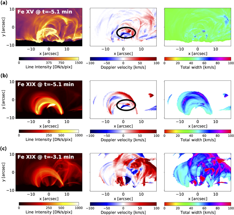
Figure 6. High-spatiotemporal-resolution rasters possible with MUSE are necessary for capturing the trigger(s) of flares and CMEs. For example, shown here are the line intensity, Doppler velocity, and total line width maps of the Fe xv 284 Å and Fe xix 108 Å lines synthesized from a radiative MHD simulation of a C-class flare (MURaM_flare, see Table 1 and Appendix A; Cheung et al. 2019). Top and middle rows: at t = −5.1 minutes, Doppler maps show bidirectional reconnection outflows at (x, y) = (0, −5)″ shown with a black circle. In this simulated flare, this coronal magnetic reconnection event is the flare trigger that destabilized the preexisting underlying magnetic flux rope. Bottom row: same as middle row but 2 minutes later.
Download figure:
Standard image High-resolution imageWhile the flare model inspired by AR 12017 featured a trigger in the coronal region above the flux rope, other simulations suggest below-the-flux-rope reconnection may be responsible. Figure 7 shows one such example. This radiative simulation (MURaM_collision) features a sunspot translating horizontally at the solar photosphere (and below), eventually colliding with a neighboring sunspot. This collision process creates a twisted magnetic flux rope above the PIL, akin to what is found in many flare-productive regions (e.g., Chintzoglou et al. 2019; Toriumi & Wang 2019b). The figure shows maps of the total intensity, Doppler velocity, and line width of the Fe xv 284 Å and Fe xxi 108 Å lines at 40 s and 20 s before the soft X-ray peak of the simulated flare. At t = −40 s, the total line width of Fe xxi shows an enhancement (of up to 100 km s−1) around the PIL (see the zoomed-in images in Figure 8). Inspection of the MHD cubes reveals this occurs below the flux rope, which is consistent with the finding of Harra et al. (2013), who reported nonthermal coronal line width enhancements from Hinode/EIS measurements at the base of three ARs before they flared. In addition, the Fe xxi Doppler map of the MHD models shows bidirectional flows in the region of enhanced line width. This is consistent with reconnection below the flux rope, i.e., tether-cutting reconnection. In general, the MUSE Fe xix line diagnostic can be used to diagnose flare triggers and map 10 MK loops and flows (Doppler and nonthermal; e.g., Figure 6). While the Fe xxi line can be used to identify triggers, it is more effective for identifying triggers (resulting in 12 MK plasma) in the lower atmosphere, close to the PIL (e.g., Figure 7). It is less effective than Fe xix for identifying triggers higher up in the corona where the temperature may be lower, or the emission measure insufficient.

Figure 7. MUSE will capture the triggering and evolution of solar eruptive events and their impact on the ambient corona. Rows (a) and (b) show the synthetic MUSE observables, namely the spectral line intensity (left column), Doppler velocity (middle), and line width (right column) for the Fe xv 284 Å and Fe xxi 108 Å lines, as synthesized from a radiative MHD simulation of a solar flare and CME (MURaM_collision; see Table 1 and Appendix A). Rows (c) and (d) show corresponding maps 20 s later. The times indicated are relative to the peak of the GOES soft X-ray light curve (as synthesized from the model). The Doppler velocity and line width maps for the Fe xxi line are overlaid over synthetic photospheric magnetograms. At t = −20 s, the bidirectional Doppler flows centered at (x, y) = (0, 0) in the hot Fe xxi line are detectable signatures of tether-cutting reconnection above the PIL, which triggers the flare and CME. The grayscale images in rows (b) and (c) show the vertical component of the photospheric magnetic field. See Figure 12 for a limb view of the same simulation.
Download figure:
Standard image High-resolution image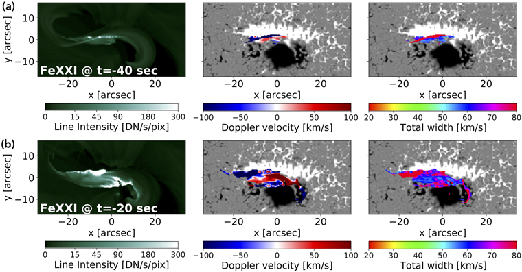
Figure 8. Zoomed-in Fe xxi 108 Å (12 MK) maps shown in Figure 7 (from model MURaM_collision; see Table 1 and Appendix A). Left: line intensity; middle: Doppler shift; and right: line width. The tether-cutting reconnection region is above the polarity inversion line (grayscale in middle and right columns shows the vertical component of the magnetic field at the photosphere). Row (b) shows the flare loop 20 s later. Unlike single-slit spectrographs, MUSE will be able to raster these FOVs with <20 s cadence to capture such dynamic changes.
Download figure:
Standard image High-resolution imageA major difference between MUSE and Hinode/EIS is the almost 2 orders of magnitude improved raster cadence of MUSE. This allows AR-scale rasters to be available at 12 s cadence, in contrast to the tens of minutes required for Hinode/EIS. An EUVST dense raster would still take several minutes to complete. In the MURaM_collision simulation, at t = −20 s (20 s after the identified trigger), a CME is already being initiated, accompanied by an EUV wave. MUSE/SG has the cadence to capture this transient phenomenon, while single-slit spectrographs would be too slow to keep up. Section 5.3 provides an extended discussion of how MUSE/SG observations of EUV waves may be used to constrain and test CME models.
While EUVST rasters at AR-scales will miss the transient/TR coronal dynamics across the FOV (e.g., see Figures 9 and 10), sit-and-stare observations or rasters with fewer steps (and thus higher cadences) would capture the thermodynamic structure of the entire atmosphere along the LOS for a narrow FOV. In the absence of large-scale context data from MUSE, it would be challenging to interpret the EUVST rasters. However, with data sets from the two observatories combined, we benefit from the spatiotemporal cadence of MUSE, as well as the temperature coverage and density diagnostics of EUVST. The photospheric and chromospheric slitjaw imaging (SJI) capability of EUVST (in the 2833 Å continuum, and 2852 Å Mg i and 2796 Å Mg ii bands; none in coronal lines) will reveal the location and morphology of preeruption prominence material and help locate the footpoints of the reconnecting field, i.e., the flare ribbons. If EUVST were rastering a region around the neutral line with the slit along the neutral line, it would be able to capture the low-T signatures of reconnection associated with tether-cutting, while MUSE can capture the upper TR and coronal reconnection across the whole FOV. EUVST/SJI will also facilitate alignment of the EUVST × MUSE data set with DKIST Visible Broadband Imager (VBI) observations. Photospheric and chromospheric magnetic field measurements will be provided by the DKIST Visible Spectropolarimeter (ViSP) and the Diffraction-limited Near-infrared Spectro-polarimeter (DL-NIRSP), and for off-limb regions, coronal field measurements by the Cryogenic Near-infrared Spectro-polarimeter (Cryo-NIRSP). Due to integration times needed, Cryo-NIRSP would only provide before and after states of the coronal magnetic field and would not provide dynamic changes during eruptions.
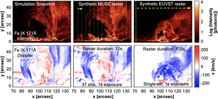
Figure 9. MUSE will capture the detailed evolution of solar eruptive events and their impact on the ambient corona. We show MUSE Fe ix 171 Å synthetic observations from a radiative MHD simulation of a solar flare and CME (MURaM_flare; see Table 1 and Appendix A). The Fe ix intensity and Doppler shift maps for a simulation snapshot (left column) are compared with corresponding line properties obtained via MUSE (middle column) or EUVST (right column) rasters. For both MUSE and EUVST we assume 04 steps and 1 s exposures for each step. For EUVST, we assume a large dense raster covering the FOV shown (∼65″ in the x-direction perpendicular to the slit(s)). MUSE high-cadence large-FOV observations would accurately capture the eruption properties. Note: The sharp jumps in the synthetic EUVST raster are due to the MHD snapshots not being saved at better than 1 s cadence past the impulsive phase of the flare. These artifacts would not appear in real observations. What would be realized in observations is the single-slit raster not capturing the dynamical evolution of the flare. In the next figure (Figure 10), we show, for the same simulation, a time series of Doppler maps obtained with MUSE and EUVST rasters.
Download figure:
Standard image High-resolution image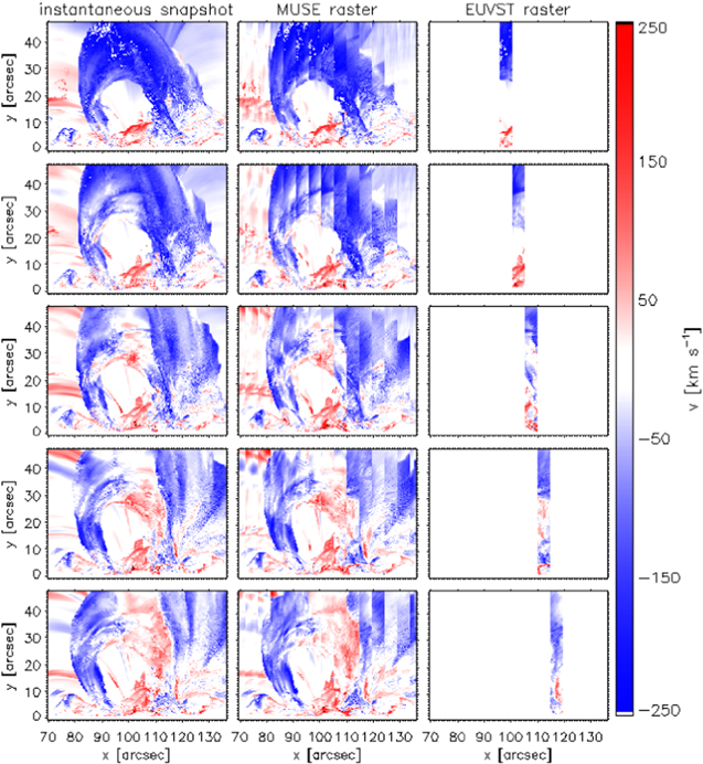
Figure 10. MUSE high-cadence spectroscopy over a large FOV is crucial for capturing the detailed dynamics of solar flares and eruptive events. For the same radiative MHD simulation of a solar flare and CME (MURaM_flare; see Table 1 and Appendix A) shown in the previous figure (Figure 9), we show a time series, covering about 1 minute overall (∼12 s for each MUSE raster) of Fe ix Doppler shift maps obtained with MUSE rasters (middle column) and EUVST rasters (right column). As in the previous figure for both MUSE and EUVST we assume 04 steps and 1 s exposures for each step, and dense rasters (i.e., 0
4 raster steps in the x-direction, perpendicular to the slit(s)).
Download figure:
Standard image High-resolution imageOne particular flare topological configuration that would be particularly well suited for MUSE observations is a circular ribbon flare with a fan–spine topology (Lau & Finn 1990). They usually occur when new magnetic flux emerges in a region of dominant field, creating a parasitic polarity that connects locally creating a quasi-spherical domain or dome of close loops (e.g., Shibata et al. 1994; Moreno-Insertis et al. 2008; Wang & Liu 2012), with a coronal magnetic null and a spine line that goes through it. In this topology, field lines from different domains reconnect at the null as emergence progresses or as an embedded flux rope becomes unstable, producing observed intensity signatures at the quasi-circular ribbon that outlines the footpoints of the fan separatrix surface, and even more interestingly at distant brightenings that point at the location of the spine footpoint. These events have been observed with imaging instruments (e.g., Masson et al. 2009; Sun et al. 2013; Hernandez-Perez et al. 2017; Xu et al. 2017) but are very challenging to be comprehensively observed with a single-slit spectrograph when the distant flare signatures at the spine are typically 100″–150″ apart from the main ribbons. MUSE is the ideal instrument to diagnose the still unknown spectral properties at the spine and circular ribbons and their spatial and temporal interdependency. The topology is uniquely favorable to characterize and understand the intensity, Doppler shift, and nonthermal signatures of magnetic reconnection at and around a null point. Figure 11 shows a circular ribbon flare observed in simulation MURaM_circ_rib. During the onset of the circular ribbon flare, MUSE observables highlight the magnetic field structure consisting of a combination of locally closed and more distantly connected loops, which is in this case more complex than the classical fan–spine structure. The Fe xv 284 Å maps show the intensity and Doppler signatures at the circular ribbon flare ([x, y] = [0, −10]) and the distant footpoints ([x, y] = [ −25, −25]″). The rapid evolution, that in the case of the Doppler signatures is at the scale of 1 minute or less, requires a fast (tens of seconds) raster scan of the AR. EUVST will be able to do a 50″–60″ dense raster of this compact example in ∼1–2.5 minutes (0.5–1 s exposures), but a typical 100″ FOV would take 2–4 minutes, both insufficient to capture the dynamics of reconnection. An EUVST sit-and-stare observation at the ribbons or fortuitously at the spine would provide a full temperature diagnostic at the appropriate cadence, at a single location. MUSE with its multiple slits, will be able to obtain diagnostics at both locations simultaneously, producing a raster of 170″ × 170″ in 12 s, making it the ideal instrument to firmly establish the spectral constraints and tests to current model predictions such as MURaM.
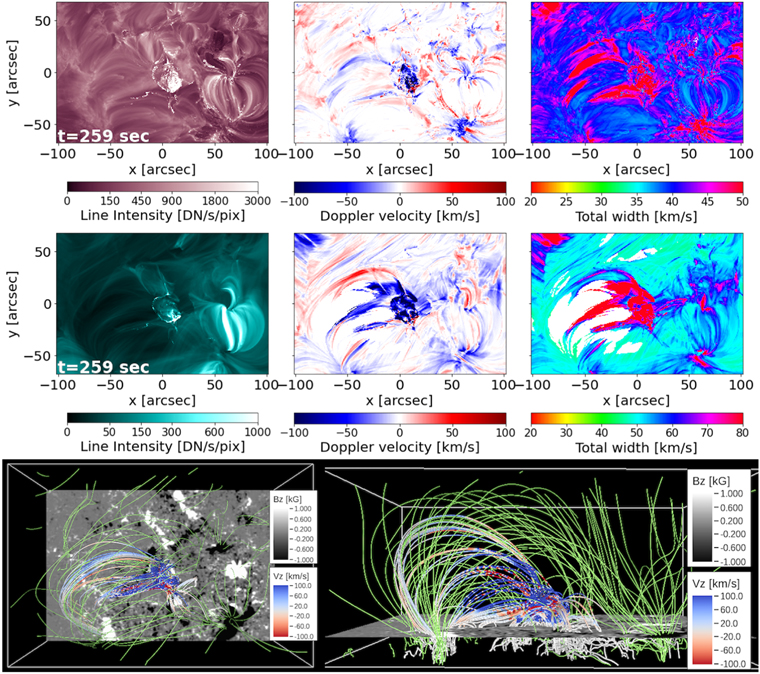
Figure 11. Top rows, left: zeroth (total intensity), first (Doppler shift), and second (line width) moments in the Fe xv 284 Å and Fe xix 108 Å lines for a simulation of a circular ribbon flare (simulation MURaM_circ_rib, see Table 1 and Appendix A; F. Chen et al. 2021, in preparation). During the onset of the circular ribbon flare, MUSE observables highlight the magnetic field structure consisting of a combination of locally closed and more distantly connected loops, which is in this case more complex than the classical fan–spine structure. Bottom row: field line traces for a top (left) and side (right) view. Field lines in green show the background field; field lines in red/blue color are selected to highlight field lines associated with the flare. They are randomly selected with a bias toward regions with a strong downward-directed conductive heat flux. The color coding is based on the vertical flow velocity and shows close correspondence to the first moments observable with MUSE in the top view. Rapid evolution requires a fast raster scan of the AR.
Download figure:
Standard image High-resolution image5.3. II-3: Understand the Evolution and Propagation of CMEs and their Effect on the Surrounding Corona
The capability of forecasting hazardous solar eruptions depends critically on how well we understand the initial physical conditions of the source region(s) of CMEs, the physical environment through which the CME develops and propagates, and the physical processes involved when the CME interacts with the ambient corona. While EUVST (with seamless temperature coverage) and DKIST (with magnetic field information) can provide useful information when observing the CME–corona interaction region, the observations of MUSE with a large FOV and at higher temporal resolution are necessary for investigating this important aspect of solar eruptions.
5.3.1. Initial Physical Conditions of CME Source Regions
There are a number of ways MUSE will improve models of CMEs. First of all, MUSE coronal imaging can be used to constrain 3D models of the coronal magnetic field (Section 5.1). This includes the identification of sigmoid-like loops (for on-disk observations), which are signatures of twisted magnetic fields (e.g., see intensity maps in Figures 2 and 7), the field structure of circular ribbon flares (see Figure 11), and coronal bubbles associated with hot flux ropes (for off-limb observations, see Figures 12 and 13).
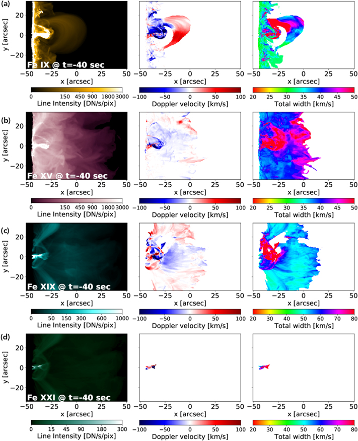
Figure 12. MUSE will capture the triggering and evolution of solar eruptive events and their impact on the ambient corona. Rows (a)–(d) show the synthetic MUSE observables, namely, the spectral line intensity (left column), Doppler velocity (middle), and line width (right column). (a): Fe ix 171 Å; (b) Fe xv 284 Å; (c) Fe xix 108 Å; and (d) Fe xxi 108 Å. These are synthesized from a radiative MHD simulation of a solar flare and CME (MURaM_collision; see Table 1 and Appendix A). See Figure 7 for a top-down (disk center) view of this model. Hot plasma (T ∼ 12 MK) is detectable in the Fe xxi line showing magnetic reconnection under the flux rope.
Download figure:
Standard image High-resolution image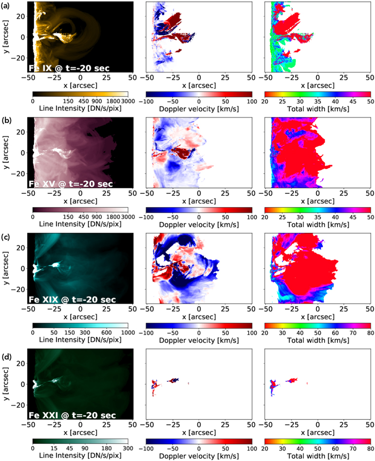
Figure 13. Same as Figure 12 but 20 s later.
Download figure:
Standard image High-resolution imageSecond, MUSE observations can help locate where and when eruption/flare triggers occur (e.g., Fe xxi 108 Å Doppler velocity and line width maps in Figure 7; Section 5.2).
Third, MUSE will provide new constraints on the early phases of CMEs to initialize data-constrained models of CMEs (e.g., Downs et al. 2012; Shiota & Kataoka 2016; Török et al. 2018). For example, consider Alfvén Wave Solar Model (AWSoM)+Eruptive Event Generator (Gibson and Low) (EEGGL; van der Holst et al. 2014; Jin et al. 2017), a module delivered to NASA’s Community Coordinated Modeling Center (CCMC) for the space weather community to run data-driven CME models. Currently, this model uses the observed CME speeds from coronagraphs as well as the photospheric magnetic field measurements from the CME source region to constrain the Gibson–Low flux rope parameters (e.g., location, size, magnetic strength, orientation, and helicity). However, the plasma properties within the flux rope are not currently constrained by observations. MUSE Doppler observations of the erupting flux rope could be used to specify the early velocity profile (e.g., the Fe xv Doppler map at t = −20 s in Figure 7) of a magnetic flux rope, which is not explicitly specified in the current model. Such Doppler maps would be particularly important for constraining the early conditions of CMEs from on-disk source regions. Such CMEs are more likely to be Earth-directed and geoeffective.
For off-limb CME source regions, the spatial distribution of the flow pattern (e.g., as shown in Figure 12) will still be used to better constrain other flux rope parameters (e.g., orientation). Furthermore, the early stage kinematic CME information (e.g., speed, acceleration) obtained by MUSE will provide important data for estimating the CME terminal speed and energetics, which are used to determine the magnetic flux of the GL flux rope in the EEGGL. Currently, this information is obtained from white-light coronagraphic observations when the CME is already at several solar radii. Obtaining this information earlier and more accurately will be critical for improving the model capability for space weather forecast purposes. Last but not least, the MUSE nonthermal line width observations will act as improved constraints on the wave heating parameters of global MHD models. For example, the current AWSoM model uses a constant heating parameter throughout the whole simulation domain (van der Holst et al. 2014). The nonthermal broadening information from MUSE will allow to apply spatially resolved wave heating parameters for the CME source region. This can impact the properties of the solar wind solution and the global magnetic topology of the ambient field. Both these effects are known to impact CME propagation and deflection (Lugaz et al. 2011; Manchester et al. 2017). Additionally, MUSE observations may reveal that wave heating is an incomplete or inadequate description of coronal heating (see De Pontieu et al. 2022, for a thorough discussion of how MUSE observables will be used to diagnose heating mechanisms). Such a finding will guide the improvements of global MHD models.
5.3.2. Interaction of Eruptions with the Ambient Corona
CME propagation can be affected by the global coronal magnetic field, as manifested, for example, in deflection and rotation (see review paper by Manchester et al. 2017). CMEs can also impact large-scale coronal structures, as seen, for example, in remote filament oscillations and sympathetic flares/eruptions (Schrijver & Title 2011; Jin et al. 2016). In order to understand the early evolution of CMEs and to obtain important information on coronal structures, we need to understand the low-coronal signatures of CMEs (e.g., EUV waves, coronal dimmings, supra-arcade downflows) and to measure velocities projected in the LOS and on the POS.
To illustrate how MUSE observations will advance our understanding of the interaction of eruptions with the ambient corona, Figure 7 shows an example of the synthetic MUSE observables from a radiative MHD simulation of a solar flare and CME (MURaM_collision; see Table 1). At t = −20 s, strong downward motions are evident outside the AR with a maximum value exceeding 100 km s−1. This phenomenon is due to the downward push of the CME during its expansion into the corona, which in rare cases has been observed by Hinode/EIS with the “sit-and-stare” mode with deep exposures of 45 s (Harra et al. 2011; Veronig et al. 2011) as well as in simulations (e.g., Jin et al. 2016). Note that the flow pattern is highly structured and varies significantly on timescales of seconds, which will provide important diagnostics about the erupting flux rope (e.g., the coronal dimming of the flux rope footpoints; see Fe xv intensity map at t = −20 s, at (x, y) = (−10, 5)″) and its interaction with the ambient corona. Therefore, while EUVST (with better temperature coverage) can provide useful information when observing the CME–corona interaction region, MUSE observations with a large FOV and at a higher temporal resolution are clearly required for investigating the nonlocal aspects of solar eruptions. MUSE will capture the timing and location of local triggers (e.g., tether-cutting, breakout reconnection) and possible remote triggers (e.g., EUV waves from other eruptions).
5.4. II-4: Understand the Processes of Fast Magnetic Reconnection
It is generally accepted that fast magnetic reconnection is necessary to power the acceleration of energetic particles, but the exact pathways by which this magnetic energy is converted into kinetic energy of particles, where the energy conversion happens, and how the energy is partitioned between thermal and nonthermal populations, is still under intense debate (Zharkova et al. 2011). Although the EUV spectral lines observed by MUSE will not directly probe plasma populations at superhot (tens of MK and above) temperatures, it will provide important observations revealing the nature of fast reconnection (e.g., the plasmoid instability), and the plasma environment in which particle acceleration takes place (e.g., the structure of termination shock regions in reconnection outflows). MUSE observations of flare ribbons can also be used as constraints on flare loop models investigating how loop atmospheres respond to injection of different particle/energy deposition mechanisms (see Section 5.4.4).
5.4.1. Plasmoid Instability in Current Sheets
In recent years, an emerging picture of magnetic reconnection suggests reconnection occurs in a dynamical fashion, unlike the earlier models of steady-state Sweet–Parker and Petschek-type reconnection scenarios. A robust result of numerical magnetic reconnection experiments at sufficiently high Lundquist numbers S ≳ 104 (S = VA
L/η, where VA is the Alfvén speed, L the system-scale length, and η the magnetic resistivity) is the formation of plasmoids (Loureiro et al. 2007; Bhattacharjee et al. 2009; Samtaney et al. 2009; Pucci & Velli 2014; Shibayama et al. 2015). Shibata & Tanuma (2001) have postulated that plasmoids exist in a spectrum of sizes exhibiting a fractal nature. These plasmoids are apparently a basic property of reconnection, seen in simulations where the initial conditions (magnetic field strength, thermodynamic variables) are symmetric or asymmetric about the current sheet (e.g., Figure 15). While bidirectionally moving (in the POS) plasma blobs resembling plasmoids have been identified in sequences of SDO/AIA EUV images (Takasao et al. 2012; see Figure 14), there exists no clear evidence that plasmoids are produced over a wide range of scales. Single-slit observations of the nonthermal broadening of TR lines by IRIS are consistent with the plasmoid instability (Innes et al. 2015), including the onset of fast reconnection mediated by plasmoids (Guo et al. 2020). However, the sit-and-stare observations used do not constrain the spatial structure and temporal evolution given the large POS motions (see also Rouppe van der Voort et al. 2017). IRIS slitjaw images have also revealed some features that could be plasmoids (Antolin et al. 2021; A. R. C. Sukarmadji et al. 2021, in preparation). With 04 resolution spectroscopic imaging data and 0
33 context imaging data, MUSE will test whether plasmoids at subarcsec scales exist and track their dynamical evolution.
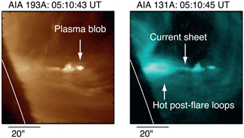
Figure 14. SDO/AIA narrowband imaging data show bidirectionally moving (in the POS) “plasma blobs” ejected from a current sheet (Takasao et al. 2012, 2016). The identified ejected plasmoids have widths of 2″–3″. MUSE will provide imaging spectroscopic observations, testing model predictions that plasmoids are produced over a range of length scales, and can coalesce and be ejected out of a current sheet.
Download figure:
Standard image High-resolution imageThe classical theory of fast Petschek reconnection involves standing slow-mode shocks across which magnetic energy is converted into kinetic energy. The fully compressible MHD simulations of Harris sheet reconnection at S ∼ 104 by Shibayama et al. (2015) predict the existence of dynamical (i.e., nonstanding) slow-mode shocks between plasmoids. They also report that the existence of these Petschek-type slow-mode shocks is efficient in removing ejecta from localized reconnection regions, which enhances the reconnection inflow. If the plasma ejecta of size ∼3″ reported by Takasao et al. (2012) were indeed plasmoids, the accompanying dynamical slow-mode shocks can potentially be mapped by MUSE, if they exist. Their discovery would provide support for the dynamical Petschek reconnection model.
EUVST, with a single slit and lacking coronal slitjaw imaging capability, will be unable to spectrally raster fast enough the elongated coronal currents to probe the highly dynamic evolution of the plasmoid instability. This observational gap will be filled by MUSE’s multislit spectral imaging capability, which will raster an FOV with comparable resolution to EUVST at 30× to 100× the cadence. As a representative example of the capabilities of MUSE, Figure 15 illustrates the formation of multiple plasmoids within an elongated current sheet (length L > 15″) in the Bifrost simulation B_npdns03. This figure also shows the plasmoids being ejected from the current sheet. In the image, the left column shows maps of the temperature T (top) and mass density ρ (bottom) at time t = 4764 s of the run. At this time, asymmetric magnetic reconnection occurs between the chromosphere and the corona leading to a hot coronal jet. In addition, the current sheet becomes unstable to the tearing-mode instability (Furth et al. 1963) and several plasmoids are created and ejected due to the imbalance of the Lorentz force. The arrows indicate the location of two such plasmoids that are ejected from the current sheet. The trajectory of the different plasmoids are distinguishable as slanted lines in the intensity spacetime plots (rightmost three columns). They are initially detectable in Fe ix 171 Å maps and then eventually in the Fe xv 284 Å maps as the reconnection proceeds because the newly created and ejected plasmoids are hotter. Moreover, inspecting these slanted lines, the X reconnection point can be identified as the location from which the plasma flows diverge in opposite directions. This is the case for the two plasmoids we have highlighted as examples: the left one moves upwards to greater coronal heights, while the right one descends toward the lower atmosphere. We can also discern the coalescence of plasmoids as they appear as almost perpendicular lines to the trajectories with changes in the Doppler shift values. In addition, in the line width panels, it is possible to know where the plasmoids impact after being ejected from the current sheet, e.g., between x = 38″ and x = 40″ and at x = 52″. This way, MUSE offers a unique capability to unravel the nature of the plasmoids as well as their coalescence and impact against preexisting magnetic field. Since plasmoids are considered possible environments where energetic electrons may be accelerated (e.g., Drake et al. 2006), the ability of MUSE to capture the evolution of plasmoids will provide important constraints for models on the possible injection time and location of nonthermal electrons (NTE). See Section 5.4.4 for further discussion.
Figure 15. Formation and ejection of multiple plasmoids within an elongated current sheet in the Bifrost simulation B_npdns03 (see Table 1 and Appendix A). The left column shows the temperature (top) and mass density (bottom) at time t = 4764 s of the run. The panels on the right contain X–t maps (computed for an LOS direction parallel to the z-axis) of the MUSE Fe ix 171 Å (top) and Fe xv 284 Å (bottom) moments, namely, the intensity, Doppler shift, and line width. The horizontal dotted line in these panels corresponds to the time shown in the temperature and density panels. An animation of the figure is also available showing the evolution of the temperature and density between t = 4602 s and t = 4946 s. The real-time duration of the animation is 7 s.
(An animation of this figure is available.)
Download figure:
Video Standard image High-resolution imageEUVST rasters of the preflare conditions will be important for establishing the physical conditions of the entire stratified atmosphere in a narrow FOV before the onset of reconnection. To probe the dynamics of the plasmoid instability in thin current sheets requires subarcsecond resolution and imaging cadence much faster than one minute. EUVST would achieve this only for very narrow rasters (e.g., 8″ wide rasters with 04 step size, 1 s slit dwell time for 20 s cadence). Since it is not known a priori where current sheets will form, the likelihood of narrow EUVST rasters capturing the events of interest will be low, as demonstrated by the fact that there are very few spectroscopic observations of the plasma sheet region with single-slit spectrometers (e.g., Warren et al. 2018a). Furthermore, lack of coronal context imaging from MUSE would make narrow rasters very difficult to interpret. This observational gap must be filled by MUSE’s multislit spectral imaging capability, which will raster an FOV with comparable resolution to that of EUVST at up to 100x the cadence, capable to scan a whole reconnection site with less than 20 s cadence. These fast spectral imaging will follow the multithermal dynamical development of plasmoids, the evolution of reconnection null points, the colliding plasmoids with the open field, and the reconnected retracting loops.
DKIST, EUVST, and MUSE coordinating as a distributed NSGPM will provide unprecedented observational constraints on reconnection physics from collisional to collisionless plasmas and from weakly to fully ionized plasmas. DKIST Cryo-NIRSP coronagraphic spectropolarimetric measurements of the Fe xiii 10746 Å, Fe xiii 10798 Å, Si x 14301 Å, and Si ix 39343 Å lines will provide diagnostics of the LOS component of the coronal magnetic field, as well as orientation of the POS components (Schad & Dima 2020). Spectropolarimetric observations by DL-NIRSP and ViSP will map the photospheric and chromospheric magnetic field, directly showing the locations of current sheets in the lower atmosphere. High-cadence imaging from DKIST VBI would also reveal whether current sheets operating in the fully collisional, weakly ionized regime produce plasmoids as predicted from multifluid numerical experiments (Leake et al. 2012). Finally, the distributed NSGPM can study reconnection between magnetic fields loaded with plasma of different temperatures (e.g., chromospheric and coronal), an example of which is shown in Figure 15 (see also Rouppe van der Voort et al. 2017). The distributed NSPGM offers the opportunity to study magnetic reconnection in such realistic scenarios (unlike the equilibrium 2D Harris sheet configuration) and reconnection between fully collisional (chromospheric) and weakly collision (coronal) plasmas.
5.4.2. Fine Structure of Termination Shock(s) and Reconnection Outflows
There is increasing evidence that the sunward-directed reconnection outflow impinging onto the flare arcade leads to the formation of a fast-mode termination shock (Chen et al. 2015, 2019; Luo et al. 2021). Recent work on modeling the 2017 September X8.2 flare and comparisons with EUV and radio observations has suggested that a termination shock is a plausible region for particle acceleration (as opposed to near the reconnection region, see Chen et al. 2020).
One spectroscopic signature predicted by the models are the deflecting flows downstream of the shock, which would be observed as large (≈200 km s−1 for Fe xxi) blue and redshifts in the spectra of high-temperature EUV/UV lines (e.g., Guo et al. 2017; see also the Fe xxi Doppler map in Figure 7 at t = −20 s). However, observations have remained very rare and elusive (e.g., Imada et al. 2013; Polito et al. 2018a), mostly due to the difficulty of observing the reconnection region at the right time, in the correct location and with the best orientation of the instrument with a single-slit spectrometer.
Some MHD models of the dynamical evolution of reconnection outflows impinging on arcade loops (Takasao et al. 2015; Takasao & Shibata 2016; Takahashi et al. 2017; Kong et al. 2019) predict the termination shock region to consist not of a single fast-mode shock but multiple interacting fast-mode shocks. The magnetic field near this region has an upward concave geometry suitable for trapping particles (so-called magnetic bottle geometry), which allows particles to be accelerated to higher energies. This is a viable model to explain coronal loop-top X-ray sources with photon energies Eph ≳ 25 keV. However, there is currently a lack of direct evidence for the multipart structure of termination shock regions.
Since MUSE/SG will capture FOVs spanning 170″ × 170″ at 12 s raster cadence (and faster for sit-and-stare and step sizes larger than 04), it will capture the evolution of flare termination shock regions with much greater chances of success than single-slit instruments. Figure 16 shows how the multipart termination shock structure in the simulation of Takasao et al. (2015) would appear as MUSE observables (at a spatiotemporal sampling rate comparable to MUSE’s capability) for a top-down (i.e., disk center) view. The coronal current sheet in the simulation is located at x = 0. The Fe xix 108 Å line shows alternating patterns of blueshifts and redshifts of approximately ±100 km s−1, a signature of the multipart termination shock structure. These regions are also accompanied by an enhanced total line width of a ∼100 km s−1 (see top left panel of Figure 21 in Appendix A). Detection of these signatures in MUSE observations of loops would support models of the multishock nature of termination shock regions. Comparison of such dynamic models of the evolution of the termination shock region with MUSE observables will constrain their magnetic geometries and evaluate their importance as sites for particle acceleration.
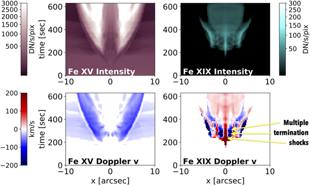
Figure 16. Synthesized MUSE observables (top-down view) from the flare arcade reconnection model Termination_shocks (see Table 1 and Appendix A) of Takasao et al. (2015). Shown are distance–time diagrams of the line intensity and Doppler shift of the Fe xv (284 Å, 2 MK; left) and the Fe xix (108 Å, 10 MK; left) lines. Interacting fast-mode shocks in the sunward reconnection outflow appear as oppositely directed Fe xix Doppler shifts (near x = 0), as well as a crisscross pattern in the Fe xix intensity. MUSE has the spatiotemporal resolution to detect this type of magnetic tuning fork structure in flares.
Download figure:
Standard image High-resolution imageIt has been proposed that such outflows are unlikely to be laminar (Larosa & Moore 1993) and are instead likely to develop a turbulent structure, which, cascading down to kinetic scales, is capable of bulk acceleration of electrons (e.g., Bian et al. 2010; Melrose & Wheatland 2014). Indeed, high-cadence imaging observations by AIA are highly suggestive of the presence of turbulence in reconnection outflows (e.g., Cheng et al. 2018). Kontar et al. (2017) inferred a timescale for electron energization in such a region on the order of 1–10 s. MUSE/CI is capable of providing TR and coronal images in the He ii 304 Å and Fe xii/Fe xxiv 195 Å bands at 033 resolution at cadences down to 8 s/4 s (dual/single channel). Furthermore, MUSE/SG sit-and-stare rasters can run at a cadence as fast as 0.5 s when targeting flares. The combined capability will characterize the intermittency of the reconnection outflows, providing evidence for dynamical reconnection, while EUVST could provide differential emission measures (DEMs) and density diagnostics with sit-and-stare or narrow raster sampling a region of the outflow, with MUSE characterizing turbulence throughout a larger volume.
5.4.3. Supra-arcades, Plasmoids and their Relations to QPPs
The origins of supra-arcade downflows (SADs), supra-arcade downflow loops (SADLs; see Savage & McKenzie 2011), quasiperiodic pulsations (QPPs; see Nakariakov & Melnikov 2009), and their relationship with each other are still under debate. QPPs might be signatures of repeated/bursty reconnection, intermittent collision of plasmoids/SADs, MHD sausage-mode oscillations, and more. They likely carry information about the energy release process in flares. MUSE spectroscopic rasters will provide an unprecedented opportunity to study SADs, SADLs, and QPPs in unprecedented detail.
The magnetic tuning fork structure in Figure 16 has been proposed as the source of QPPs emanating from flare loops (Takasao & Shibata 2016). The interacting fast-mode shocks generate oscillations that radiate away from the termination shock region. An alternative explanation proposed as the driver of QPPs is the intermittent collision of plasmoids ejected from the current sheet colliding with flare arcade loops (Samanta et al. 2021). MHD waves (fast sausage modes) are yet another possible explanation for QPPs.
Using narrowband EUV imaging data from SDO/AIA (Samanta et al. 2021; see Figure 17) reported the detection of episodic temperature and density enhancements in a flare arcade following the apparent collision of SADLs with the arcade loops. The authors propose that individual QPP are driven by the collision of retracting SADLs with the underlying arcade. SADs and SADLs have typical speeds of hundreds of km s−1 and are spatially and temporally intermittent. Single-slit spectroscopic rasters with cadences of a few minutes are insufficient to track their evolution. Furthermore, flare arcade loops are not typically straight in the POS. So it is very difficult to catch the evolution of plasma along flare loops when operating a single-slit experiment in sit-and-stare mode. MUSE’s multislit approach addresses the need to capture the dynamics of SADs, SADLs, and QPPs at sufficiently high spatiotemporal cadence to test models of their physical origin.
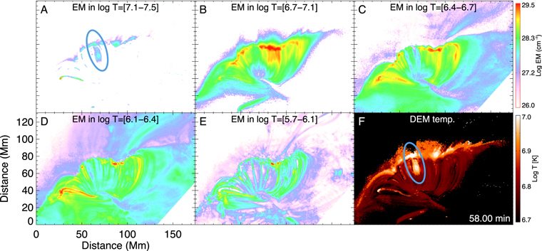
Figure 17. AIA observations of flare loops and supra-arcades show dynamical structures with spatial coherence parallel, and across neighboring flare loops. For example, this DEM map of such a system (figure from Samanta et al. 2021) shows emission measure enhancements (see oval in panel A) along loops with width down to the AIA resolution (∼1″), as well as cross-loop extensions spanning several Mm. Spectroscopic imaging data by MUSE at 04 resolution will probe whether these enhancements have signatures of termination shocks predicted by MHD models (see, e.g., Figure 16).
Download figure:
Standard image High-resolution imageMagnetoacoustic waves, in particular fast sausage modes, are another possible interpretation for QPPs (Li et al. 2020). Tian et al. (2016) attempted to detect oscillations of the width of the Fe xxi line observed by IRIS. However, the cadence was not fast enough to observe the expected line width oscillation, or perhaps the location of the slit was not ideal. The multislit coverage of MUSE will be able to capture such a line width oscillation, if it exists.
5.4.4. Heating and Magnetic Evolution at Flare Ribbons
The coronal magnetic reconnection that facilitates energy release in flares leads to intense heating of the lower solar atmosphere, up to temperatures normally considered as “coronal” (e.g., Fletcher et al. 2013; Graham et al. 2013). This results in the appearance of flare ribbons in the EUV, UV, and optical wavelengths (e.g., Isobe et al. 2007; Fletcher et al. 2011; Yadav et al. 2021). Studying these ribbons helps bridge the gap between the reconnection and the eventual dissipation of the energy that is released. It is particularly important to observe flare ribbons at subarcsecond resolutions since ground-based Hα observations of coronal rain in flare indicate loop widths as low as ∼100 km (Jing et al. 2016). In the standard 2D flare picture (Hirayama 1974), ribbons occur at the interface between distinct magnetic volumes, forming a topological discontinuity. In the 3D extension to the flare model (e.g., Janvier et al. 2015), conjugate footpoints of ribbons not only separate as new flux is reconnected, they also have a displacement along the direction of the PIL due to slipping reconnection. In both 2D and 3D cases, the topological change in the field results in reconnected field lines that can relax to a lower energy state. The Lorentz force work due to the field relaxation provides power to heat loops. Properly tracking the evolution of these loops (and thus the energy sources) in 3D requires high-cadence spectral imaging observations over AR-scale FOVs.
Combining flare ribbon observations with measurements of the magnetic field and its variation during flares gives direct information on the overall rate of flux transfer associated with magnetic reconnection (e.g., Fletcher & Hudson 2001; Qiu et al. 2002). Using 1600 Å imaging data from SDO/AIA and Transition Region and Coronal Explorer (TRACE), for example, correlation studies of the intensity and magnetic reconnection rate have been made on the scale of ARs but for individual bright features within ribbons; e.g., in Temmer et al. (2007), 2 s cadence data from TRACE was used to demonstrate that parts of the ribbon where a high reconnection rate is measured are associated with the most energetic sources—i.e., the hard X-ray emitting regions (Fletcher 2009). These studies were possible only because of the high time resolution available in optical, UV, and hard X-ray imaging observations.
Different energy transport and heating mechanisms result in distinctive thermal and dynamical properties at the flare ribbons. For example, evaporative upflows arising from heating by high-energy electrons are predicted to have a different behavior as a function of time from those due to conductive heating, as shown in simulations discussed below (Figure 19). High time resolution is critical: hard X-ray timescales for impulsive energy input are at least as short as 10 s, and the simulations suggest that transient phenomena at flare onset can be a distinguishing feature of different heating models. Previous IRIS sit-and-stare observations at 1.7 s cadence also captured the rapid onset of transition-region flows and line broadening preceding the flare heating by some 10 s, posing a challenge for our understanding of lower atmosphere energization (Jeffrey et al. 2018). The large FOV of MUSE will give simultaneous access to different parts of the flare ribbons on a spatial scale large enough to examine whether different energy transport mechanisms dominate at different times and locations in the flare (e.g., nonthermal electrons in at the strongest footpoints during the impulsive phase versus widespread conductively driven evaporation later on) and with a temporal and spatial resolution sufficient to capture ribbon variability. Coupled with magnetic field measurements over the DKIST/VTF FOV and EUVST spectroscopy providing additional plasma diagnostics over a narrower FOV, rapid progress on flare energy transport and its relationship to magnetic restructuring can be expected.
We demonstrate via flare radiation hydrodynamic (RADYN; see Section 3 and Appendix A) modeling how MUSE observations of hot flare plasma at high spatiotemporal resolutions will shed light on the partition of energy following fast reconnection.
Comparisons between models and spectroscopic observations have been shown to provide crucial diagnostics of the heating mechanisms at play in flares (e.g., Reep et al. 2015; Polito et al. 2016, 2019; Kerr et al. 2020b, 2021, to cite just a few recent results). We illustrate this by comparing the MUSE synthetic spectral observables for field-aligned modeling experiments, in which a 1D model atmosphere heated by an electron beam is mapped onto a 2D semicircular loop. The geometry is shown in Figure 11 of De Pontieu et al. (2022). Synthetic MUSE Fe xv 284 Å and Fe xix 108 Å observables for two experiments with two different preflare atmospheres are shown in Figure 18. The plasma response to the flare heating can vary significantly depending on the initial physical conditions (temperature and densities) of the preflare loop atmosphere. When the NTE are released in an initially emptier and cooler loop, the footpoint brightenings are characterized by brighter and broader lines, and larger flows compared to the denser and hotter initial atmosphere. This shows the importance of providing constraints on the initial physical conditions of the loop when diagnosing different heating models from the observations. MUSE, thanks to its multislit design, will allow to capture simultaneous spectral images of the loops prior to and after the flare.
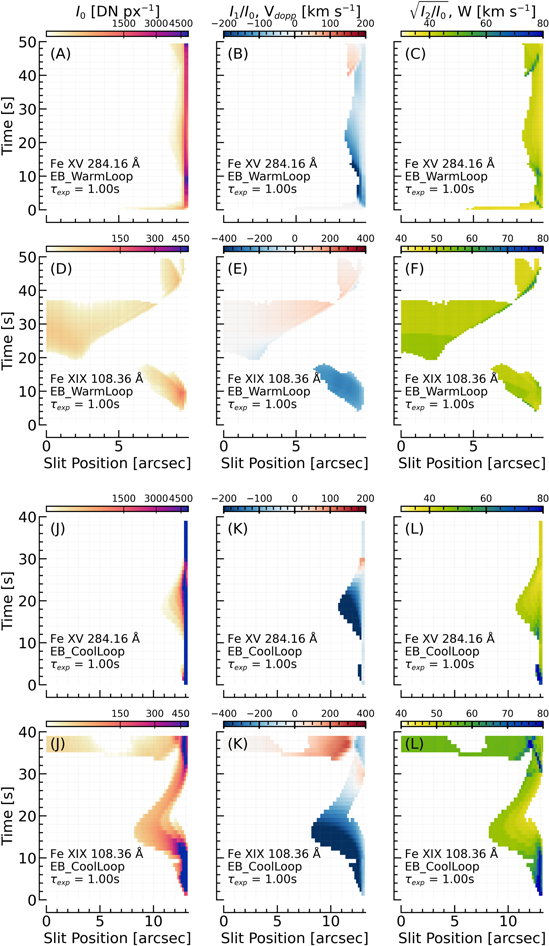
Figure 18. MUSE spectral observations both before and during the flare will provide tight constraints on the properties of the heating and flare energy transport. Shown are the moments (see Appendix C) of the MUSE Fe xv and Fe xix lines synthesized from two RADYN flare simulations with the same injected electron beam properties but with different preflare conditions (see text and Appendix A for details): model RADYN_warm_EB (panels (A)–(F)) and model RADYN_cool_EB (panels (J)–(L)). The half-loop is oriented perpendicular to the MUSE slit direction and viewed from above.
Download figure:
Standard image High-resolution imageWe also experimented with in situ heating in the corona, with the thermal conductive flux subsequently heating the transition region and chromosphere, and with a tandem experiment containing both in situ heating plus electron beam energy deposition (with the same parameters as the individual heating scenarios). In Figure 19, we compare the MUSE Fe xv 284 Å and Fe xix 108 Å synthetic spectra as a function of time for the three heating models (i.e., electron beam, EB, in situ, and in situ + EB), given the same initial physical conditions (warm and dense loop). The synthetic spectra exhibit several distinctive differences between the models. For instance, panels (B) and (E) show that the Fe xv line is brighter at the loop footpoints in the in situ and hybrid scenarios than in the EB model. In addition, in the in situ model the spectra are redshifted at the footpoint by up to 50 km s−1 in the first few seconds of the simulation. The redshift is more modest (only 5–10 km s−1) or absent in the hybrid and EB cases, respectively. Another interesting feature is the fact that the hotter Fe xix is brightest in the in situ and hybrid models, which are more effective at heating the corona to higher temperatures than the EB only case, where the electrons deposit their energy mostly in the lower atmosphere. While the loops shown here have an average length of ≈20–30 Mm, longer flare loops (up to ≈100 Mm or even longer) are also observed (e.g., Polito et al. 2019). For those cases, the large FOV coverage of MUSE is even more crucial for fully capturing all the dynamics across the loop arcade.
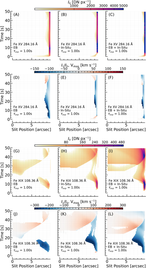
Figure 19. The timings and locations of flare responses in each line vary depending on the flare heating, making it important to have comprehensive spatial coverage on short timescales. We show the first and second moments (see Appendix C) of synthetic MUSE lines (Fe xv 284 Å and Fe xix 108 Å in the top and bottom two rows, respectively), from three RADYN flare simulations with different flare heating models (see Appendix A for details on the models shown here): an EB-driven flare (RADYN_warm_EB; left column), a flare driven by in situ coronal heating (RADYN_warm_TC; middle column), and a tandem EB plus in situ scenario (RADYN_warm_EB_TC; right column).
Download figure:
Standard image High-resolution imageIt has been proposed that in addition to nonthermal particles and in situ heating, energy may be transported during flares by high-frequency Alfvénic waves, propagating downward from the reconnection site (Emslie & Sturrock 1982; Fletcher & Hudson 2008; Russell & Fletcher 2013; Kerr et al. 2016; Reep & Russell 2016; Reep et al. 2018). Indeed, some studies (e.g., Reep et al. 2020) suggest that NTEs by themselves are insufficient in explaining all of the observed phenomenon in flares. See also Kerr et al. (2020a).
Flare simulations with energy transported via high-frequency Alfvén waves have been successful in heating the lower atmosphere and driving chromospheric ablations. However, the study of their role in flares is hampered by the lack of observational constraints on the wave properties, in particular the energy flux they carry. MUSE offers a means to constrain this Poynting flux by measuring the nonthermal width of several spectral lines at high spatial and temporal resolution.
Figure 20 shows that including broadening due to Alfvén waves can result in line widths that exceed those in which only thermal motions and LOS superposition of field-aligned flows (e.g., along different loops) are considered. This RADYN_Arcade (Kerr et al. 2020b; see Appendix A) simulation grafts RADYN field-aligned flare atmospheres onto observed AR loop structures. We include the additional nonthermal broadening that would be present if Alfvén waves were propagating during the flare, assuming in this case a Poynting flux of 1 × 10¹⁰ erg s−1 cm−2. Each MUSE spectral line experiences a different degree of nonthermal broadening due to the dependence of this broadening on the atmospheric properties through which the wave propagates along the loop. Tracking the nonthermal line broadening over time and space with the high resolution afforded by MUSE could therefore allow constraints on the energy carried by MHD waves during flares.
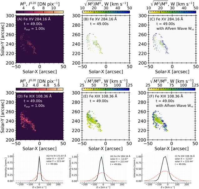
Figure 20. Illustration of the impact of nonthermal broadening due to presence of Alfvén waves during the flare. The second moment of the Fe xv 284.4 Å line (top row) and Fe xix 108.3 Å line is shown in the case with and without Alfvén wave broadening. The bottom row shows the difference in line width without Alfvén waves (black lines) and with Alfvén waves (red dashed lines) from a single pixel near a loop footpoint. By simultaneously observing conjugate footpoints, loops, and loop apexes,MUSE can study the spatial distribution of nonthermal broadening, which can be compared to models of flares that include Alfvénic waves.
Download figure:
Standard image High-resolution imageMUSE will provide essential spectroscopic images of the flaring corona with a large spatial coverage, required to fully appreciate EUVST, DKIST, and other GBO observations of the flaring chromosphere, the source of evaporated material.
Fast, but narrow, rasters with EUVST will capture smaller segments of the flare ribbons, with an emphasis on detailed plasma diagnostics to complement those from MUSE. Density diagnostics of heated ribbon plasma can be carried out, for example, using the density pairs C iii λ 977/1176 Å and Fe x λ 175/177 Å, and the sequence of Fe lines between Fe ix and Fe xiv will be used to provide DEM measurements (e.g., Baker et al. 2015, 2018). The nonthermal line widths and Doppler shifts from lines formed at different temperatures will also provide information about gradients and the stratification of flows and turbulence throughout the atmosphere.
DKIST/VBI observations will provide photospheric and chromospheric imaging, to track the overall ribbon spatial and temporal evolution. Blue continuum and G-band “quasi-white-light” images will reveal the locations where the flare kernels are the brightest, hence the locations of strongest energy deposition. VBI will also allow to follow in detail the dynamics of the ribbons by identifying/tracking features within them, to obtain the local reconnection electric field and flux transfer rate (aka “reconnection rate”; Kazachenko et al. 2017). In addition, DKIST/VTF will provide photospheric and chromospheric spectropolarimetry in Fe i 630.2 nm and Ca ii 854.2 nm, respectively, which will track the evolution and reorientation of the magnetic field as the the flare ribbons expand and travel across the AR while the coronal reconnection occurs. This will permit the identification of sites of strong discontinuities in the magnetic field, indicating possible current sheet locations.
To summarize, the large FOV and high-cadence spectroscopy of MUSE is necessary to follow the ribbon evolution over a significant area to (i) calculate the flux transfer rate over a significant portion of rapidly moving ribbons; (ii) identify conjugate footpoints from their correlated time evolution; (iii) disambiguate the spatial and temporal ribbon evolution; (iv) track in detail the onset of mass flows as a flare starts, and their relationship to flare ribbon brightening and field evolution; (v) examine the development of nonthermal line broadening, possibly due to turbulence, MHD waves, or nonthermal electrons, before and during ribbon brightening, and their spatiotemporal relationship to changes in the magnetic field. This is not possible with single-slit instruments. First, projections of loops in the POS are unlikely to lie along the slit. This means that sit-and-stare observations are insufficient. The alternative, namely, spatial rasters, is inadequate due to the long raster times of single-slit instruments. Nonspectroscopic instruments like SDO/AIA and Solar Orbiter/EUI do not have the spectral diagnostics to measure Doppler flows and nonthermal widths. For these reasons, the multislit capability of MUSE presents a unique advantage for tracking flare ribbon evolution.
5.5. II-5: Understand the Formation Mechanism of Sunspots, in Particular Delta Sunspots
Regardless of whether an AR has sunspots that are delta-type (and prone to flares), the spots do not form as newborn monolithic structures. Rather, interaction with subsurface convective flows leads to a fragmented emergence, and subsequent reorganization (opposite polarity patches counterstreaming, e.g., Pariat et al. 2004) into larger structures that eventually become sunspots (Cheung et al. 2010; Rempel & Cheung 2014; Chen et al. 2017; Toriumi & Hotta 2019a). The counterstreaming polarities drive reconnection events in the photospheric/chromospheric layers that can reach TR temperatures with broad profiles observed by IRIS (e.g., Peter et al.2014; Young et al. 2018). They are considered signatures of reconnection of sea-serpent field lines, which are field lines emerging into the solar atmosphere, modulated by granulation flows. This reconnection allows the emerging magnetic field to remove its mass burden (Cheung et al. 2010). This process allows new coronal loops to form, eventually connecting the two opposite polarity nascent sunspots. Rapid-cadence MUSE rasters of the corona above such emerging flux regions will reveal how the newly formed loops are structured. In addition, the large FOV and high-cadence raster scans will greatly increase the probability (compared to single-slit spectrographs) of capturing the initial stages of newly emerging flux and the resulting coronal response. Studying such regions with MUSE will reveal how mass is unloaded from emerging flux regions, test whether magnetic buoyancy instabilities are at play in transporting magnetic flux to coronal heights (see review by Cheung & Isobe 2014), and whether sunspots of opposite polarities are eventually connected.
Although radiative MHD numerical simulations are able to model entire sunspots with umbral and dynamic penumbral filaments (Rempel et al. 2009), there are still many open questions with regards to how the penumbra is formed and sustained. The current simulations with fully fledged penumbral filaments start from initial conditions consisting of a monolithic funnel of magnetic field introduced into an originally weak-field convecting environment. Rempel (2011) reported that artificially increasing the field inclination at the top boundary (located at the top of the photosphere) forced the model sunspot to have an extended penumbra. When the artificial forcing is switched off and the top boundary field is matched to a potential field, the model penumbra diminishes. However, a recent study concluded that model sunspots without artificial forcing at the top boundary had photospheric magnetic distributions that are more consistent with observations (Jurcák et al. 2020). Yet, those models without artificial forcing also lack extensive Evershed flows. In a study of where penumbral filaments begin to form around the periphery of nascent sunspots, Murabito et al. (2018) reported roughly half the sunspots have penumbrae forming in the region between the opposite polarity spots, while the remainder had penumbrae forming at the outer edges (i.e., opposite side from emerging flux region).
Subarcsecond MUSE intensity images from the SG and CI will be important for constraining the geometry and 3D structure of the coronal field before, during, and after the formation of penumbrae (e.g., either as inputs to extrapolation models, or as validation of models; see Section 5.1). Furthermore, spectroscopic observables like the Doppler velocity and line width can be used to track how umbral and penumbral waves (from DKIST/GBOs and EUVST) propagate into the corona (e.g., Zhao et al. 2016). For an extended discussion of wave models of coronal loops and predicted MUSE observables, we refer the reader to the companion paper on coronal heating (De Pontieu et al. 2022).
A particular class of sunspots that form the focus of NGSPM SO II-5 is the class of delta sunspots. The characteristic size of delta spots span the spectrum of AR sizes (up to 100 Mm) and the associated collisional polarity inversion lines (cPILs) range from 10 to 100 Mm (Liu et al. 2021). Photospheric and subsurface flows pressing strong (umbral/penumbral) fields of opposite polarity into a compact region drive a plethora of dynamic phenomena in the overlying atmosphere. In particular, delta sunspots are known to be particularly flare productive (e.g., see Toriumi & Wang 2019b, and references therein).
EUVST would be able to provide AR-scale rasters of delta-spot regions at a cadence of minutes (assuming 1 s slit dwell time and 04 step size for dense rasters). Continuous coverage of the AR over hours and days would allow for monitoring of the detailed thermal structure of the AR from the photosphere to corona. However, delta-spot regions often produce multiple flares and eruptions as flux emerges and as shearing and flux cancellation along the PIL ensue. As illustrated in Figures 9 and 10, single-slit spectrographs miss the important dynamics of flares and eruptions. This gap is filled by the high-cadence (<20 s), 0
4 resolution rasters of MUSE. Within smaller FOVs of what MUSE would cover, EUVST would provide seamless temperature coverage from 10,000 K to 15 MK, as well as density diagnostics.
Delta-spot regions often spawn homologous eruptions (e.g., Cheung & DeRosa 2012; Li & Zhang 2013; Panesar et al. 2016; Polito et al. 2017; Sun et al. 2017; Mitra et al. 2020). To piece together a quantitative picture of the family of homologous flares/eruptions, it is important to capture the evolution and structure of all the homologous events in their entirely via MUSE's multislit approach. This would then permit one to study how the eruptions vary throughout the evolution of the AR. As for the trigger mechanisms, Section 5.2 discusses in detail how MUSE spectral moment maps can be used to identify the location and timing of triggers.
6. Conclusions
In summary, no spectroscopic observations have ever been captured at the spatiotemporal scales characteristic of the corona. The highest-resolution coronal data to date are based on imaging, which is blind to many of the processes that drive coronal energetics and dynamics. As shown by IRIS, Hinode, and GBOs for the low solar atmosphere, we need high-resolution spectroscopic measurements with simultaneous imaging to understand the dominant processes. EUVST will provide subarcsecond resolution spectra with seamless temperature coverage from the photosphere to the flaring corona, but due to its single-slit design and the lack of context/slitjaw coronal imaging, it will not be able to raster AR-scale regions with sufficient cadence to freeze coronal dynamics (see, e.g., Figures 9 and 10), especially during flares and eruptions. MUSE provides the essential spectroscopic imaging capability at high resolution and cadence to capture EUV waves, CME triggering events, and plasmoids (if they exist) on a routine basis. These observations are necessary to discriminate models of flares/eruptions, to detect signatures of turbulent structure in current sheets and reconnection outflows, and to constrain physics-based space weather models.
As case studies in Section 5 demonstrate, coordinated observations between MUSE, EUVST, and DKIST (and other GBOs with subarcsecond spectropolarimetric capabilities) can be considered as a distributed implementation of the NGSPM mission concept. This distributed mission can tackle the NSGPM science objectives to understand how energy accumulation occurs in ARs, how flares and eruptions are triggered (e.g., Figures 6 and 7), how CMEs evolve from their source region to interact with the ambient corona (Figures 7, 12 and 13), how to characterize the consequences of fast magnetic reconnection (e.g., multishock structure in the termination shock region, see Figure 16); electron beam footpoint heating (e.g., in flare ribbons; see Figure 19), and how sunspots (especially delta spots) form. Table 3 lists the relevant physical phenomena and predicted MUSE diagnostics. The combined capabilities of the NSGPM will also provide unprecedented insight into the source regions of disturbances and waves in the heliosphere as measured by the Parker Solar Probe, Solar gOrbiter, and planetary missions with instruments monitoring space weather conditions in the solar system.
Table 3. MUSE Diagnostics for Eruptive and Flaring Events for Case Studies Addressing NGSPM Science Objectives II-1 to II-5 (see Table 2)
| SO | Physical Phenomena | Predicted Diagnostic/Observational Constraint | λa (Å) | Figures |
|---|---|---|---|---|
| II-1 | - Quasi-separatrix layer | - ∼10–20 km s−1 blueshifts in fan loops at edge of AR | 284 | 4 |
| - Emerging flux | - Loops connecting opposite polarities with alternating blueshifts and redshifts of tens of km s−1 | 171, 284 | 3 | |
| - Sheared field near PILs | - Loop morphology constraints (e.g., sigmoidal loops) | 195, 284, 108 | 2, 7, 8 | |
| II-2 | - Triggers of flares and eruptions | To distinguish between flare/CME initiation models: location and timing of transient bidirectional flows, brightenings, and enhanced nonthermal width identifying the reconnection site | 284, 108 | 6–8, 12–15 |
| II-3 | - Preeruption coronal field structure | - Sigmoidal loops, elliptic or teardrop-shaped coronal cavity/bubble, hot flux ropes (see Table 1 of Patsourakos et al. 2020) | 171, 195, 284, 108 | 2, 7, 8, 12, 13 |
| - CME-ambient corona interaction (including sympathetic eruptions and flares) | - EUV wave front and ambient coronal response | 195, 284, 108 | 7, 13 , 11 | |
| - Redshifted loops in ambient corona from CME expansion | 284, 108 | 7 | ||
| - CME source region | - Doppler shift maps of early CME rise to constrain flux-rope driven CME models | 171, 284, 108 | 7, 13 | |
| - Coronal heating | - Spectral line intensities and line widths as constraints on ad hoc heating terms in global MHD models with Alfvén wave heating | 171, 284, 108 | ||
| II-4 | - Plasmoid instability | - Plasma blobs in intensity images, spectral rasters | 171, 195, 284, 108 | 14, 15 |
| - Trajectory and thermal evolution of plasmoids | 171, 195, 284, 108 | 15 | ||
| - Coalescence of plasmoids from Doppler maps | 284, 108 | 15, 19 | ||
| - Enhanced line broadening | 284, 108 | 15, 18, 19 | ||
| - Multipart termination shock structure | - Alternating, pulsating patterns of blue and redshifts | 108 | 16 | |
| - Plasmoid impact on arcade loops | - Reconnection outflows impinging on arcade loops | 108 | 17 | |
| - Loop heating mechanisms | - Spatiotemporal evolution of spectral moments along loop (including footpoints) constrains heating properties (in situ, NTE) | 284, 108 | 19 | |
| - Line widths provide constraints on Alfvén wave flux | 284, 108 | 20 | ||
| II-5 | - Formation of delta spots | - Sigmoidal loops | 195, 284, 108 | 7, 11 |
| - Penumbra formation | - Coronal loop morphology | 171, 195, 284 | ||
| - Umbral/penumbral waves | - Tracking of waves into the corona from Doppler and line width maps | 171, 284 | ||
Notes. PIL: Polarity inversion line. NTE: Nonthermal electrons.
a For 304 and 195 Å, imaging is desired. For 171, 284, and 108 Å, the intensity, Doppler shift, and line broadening are typically desired. Note that when referring to the 108 Å spectral band we typically refer to both the Fe xix 108.35 Å and Fe xxi 108.12 Å lines.Download table as: ASCIITypeset image
Understanding the complex dynamics in the turbulent solar atmosphere requires not only high-cadence, high-resolution observations and spectral diagnostics but also advanced numerical simulations. A core component of the MUSE science investigation involves the use of numerical models, for the following reasons. First of all, MUSE (and, in general, the NGSPM) observations will allow us to test, discriminate, and improve existing models. Second, they guide the team to develop the science requirements that flow down to the instrument requirements. It is through this process that we identify the need for high-cadence imaging and show how single-slit spectrographs like EUVST (which, complementarily, have better temperature coverage and diagnostics of density and chemical composition) would miss important dynamics and the relevant context. The simulations used in this and a companion paper are just a subset of what can be done to compare models with MUSE observations. The purpose of the MUSE mission, and of this paper, is not to show that existing models are correct. Rather, MUSE will provide the necessary measurements at the appropriate cadence and resolution to test our understanding of solar eruptive activity, to discriminate between models, and to build a solid foundation for physics-based models of flares and CMEs. The combined capabilities of the NSGPM will also provide unprecedented insight into the the source regions of disturbances and waves in the heliosphere as measured by the Parker Solar Probe, Solar Orbiter, and planetary missions with instruments monitoring space weather conditions in the solar system.
We would like to thank Amy Winebarger, Stuart Bale, Harry Warren, Toshifumi Shimuzu, Lars Frogner, Charles Kankelborg, Jenna Samra, Sami Solanki, Hardi Peter, Jorrit Leenaarts, Paolo Pagano, Fabio Reale, Peter Young, and Wei Liu for their valuable contributions and discussions of the results. We are grateful to Jim Lemen for his technical leadership in the MUSE investigation. We gratefully acknowledge support by NASA contract 80GSFC21C0011 (MUSE Phase A). Some of this work was also supported by NASA contract NNG09FA40C (IRIS) and NASA grants 19-HTMS19_2-0025, 80NSSC18K1285, 80NSSC21K0737, and 80NSSC19K0855. D.N.S. acknowledges funding from the Synergy grant No. 810218 (ERC-2018-SyG) of the European Research Council and the project PGC2018-095832-B-I00 of the Spanish Ministry of Science, Innovation, and Universities. P.A. acknowledges funding from the STFC Ernest Rutherford Fellowship (No. ST/R004285/2). V.P. acknowledges support from NASA’s HGI grant# 80NSSC20K0716. L.F. acknowledges support from STFC Consolidated Grant ST/T000422/1. G.C., M.R. and MCMC acknowledge support from NASA grant 80NSSC19K0855 “Investigating the Physical Processes Leading to Major Solar Activity.” M.C.M.C. acknowledges support from NASA’s SDO/AIA contract (NNG04EA00C) to LMSAL. AIA is an instrument on board SDO, a mission for NASA’s Living with a Star program. G.S.K. acknowledges support from NASA’s Early Career Investigator Program (Grant# 80NSSC21K0460) and Heliophysics Supporting Research program (Grant# 80NSSC19K0859). The simulations have been run on clusters from the Notur project, and the Pleiades cluster through the computing project s1061, s8305, and s2169 from the High-End Computing (HEC) division of NASA. This material is based upon work supported by the National Center for Atmospheric Research, which is a major facility sponsored by the National Science Foundation under Cooperative Agreement No. 1852977. We would like to acknowledge high-performance computing support from Cheyenne (doi:10.5065/D6RX99HX) provided by NCAR’s Computational and Information Systems Laboratory, sponsored by the National Science Foundation. S.D. is supported by a grant from the Swedish Civil Contingencies Agency (MSB) and the Knut and Alice Wallenberg foundation (2016.0019). Simulation MURaM_emergence was performed on resources provided by the Swedish National Infrastructure for Computing (SNIC) and the European Union's Horizon 2020 research and innovation program under grant agreement No. 824135 (SOLARNET). The synthesis and analysis of the various numerical models have been performed on the Google Cloud Platform, allowing sharing the synthetic data and models, developing common tools, and access to instances with various specifications and Graphics Processing Units (GPUs). This project has been supported by a grant (project lunar-campaign-29341) by Google Could to the University of Oslo.
To analyze the data we have used IDL, Python, and PyTorch (Paszke et al. 2019). This research is also supported by the Research Council of Norway through its Centres of Excellence scheme, project number 262622, and through grants of computing time from the Programme for Supercomputing. IRIS is a NASA small explorer mission developed and operated by LMSAL with mission operations executed at NASA Ames Research Center and major contributions to downlink communications funded by ESA and the Norwegian Space Centre.
Appendix A: Numerical Simulations
Throughout the paper, we presented synthetic observables from several numerical models, listed in Table 1 of Section 3, and for which here we provide a description.
MURAM. The MURaM code aims to address the most relevant physical processes in the outer solar atmosphere, i.e., photosphere, chromosphere, TR, and lower corona. MURaM can cover a spatial range from deep in the convection zone to a coronal scale height (∼50 Mm) or more. The simulations presented here are based on the coronal extension of the MURaM code as described in Rempel (2017) and include the following: single fluid MHD, 3D gray radiative transfer, a tabulated LTE equation of state, Spitzer heat conduction, and CHIANTI-based optically thin radiative loss in the corona. As for the Bifrost experiments, the Poynting flux that heats the chromospheric and coronal parts of the simulation domain is generated through magnetoconvection in the photosphere and convection zone. Here we analyze several different simulations (see Table 1):
- 1.Model MURaM_flare: This is a 3D radiative MHD simulation of a solar flare inspired by the evolution of AR 12017. The region spawned dozens of flares (Cs, Ms, and one X-class flare) as a parasitic bipole emerged near the preexisting leading sunspot. The MHD simulation mimics this process and created a C4 flare. See Cheung et al. (2019) for details.
- 2.Model MURaM_circ_rib: This model is based on the flux emergence setup of Chen et al. (2017) that couples a global dynamo simulation (Fan & Fang 2014) with MURaM. This work was extended into the corona, resulting in a 197 Mm wide domain reaching 113 Mm above the photosphere, as will be detailed in F. Chen et al. (2021, in preparation). We did not specifically set up the simulation to produce a circular ribbon flare; the conditions just arose as part of a complex flux emergence process. The analysis shown in Figure 11 is restricted to a subdomain of 147 × 98 × 66 Mm3.
- 3.Model MURaM_emergence is aimed at simulating the plasma dynamics in an emerging flux region (see Figure 3). The simulation domain has an extent of 40 × 40 × 22 Mm, with 8 Mm protruding below the photosphere. The resulting model is generated in phases, similarly to previous runs. The initial magnetic field of 200 G is added to well developed nonmagnetic convection simulation to form extended magnetic field concentrations at meso- to super-granular spatial scales. The computational domain was then extended to include the upper solar atmosphere and the magnetic field from the preexisting simulation was used for potential field extrapolation into the rest of the domain. The new simulation was then run until a relaxed state is achieved (Danilovic 2020). In this model, the additional bipolar flux system is advected through the bottom boundary over an ellipsoidal flux-emergence region with the major axes (a, b) = (3, 1) Mm and B0 = 8000 G field strength (Cheung et al. 2019). The emergence resulted in a flare after 4.6 hr of solar time. Earlier, low-activity phases of this simulation are analyzed in the companion paper to this, which studies coronal heating (De Pontieu et al.2022).
Bifrost. The Bifrost models cover a domain that ranges from the convection zone up to the corona, include self-consistent magnetoconvection, and self-consistently produce a chromosphere and hot corona, through the Joule dissipation of electrical currents that arise as a result of footpoint braiding in the photosphere and convection zone (Hansteen et al. 2015). Bifrost (Gudiksen et al. 2011) solves the MHD equations, including thermal conduction along the magnetic field, non-LTE and nongray radiative transfer with scattering (Hayek et al. 2010; Skartlien 2000), parameterized radiative losses (Carlsson & Leenaarts 2012) in the upper chromosphere, TR, and corona, and characteristic boundary conditions on the upper and lower boundaries. Optically thin radiative losses in the corona are based on CHIANTI emissivities (e.g., Del Zanna et al. 2021)
The main free parameter for these simulations is the seed magnetic field (and its spatial distribution and strength), which can produce drastically different atmospheres (Hansteen et al.2010).
The Bifrost model we use here (B_npdns03; see Table 1 and Figure 15) is a 2D simulation aimed at studying coronal bright points and their conspicuous emission in EUV and X-rays. The initial condition was created imposing a potential null-point configuration at 8 Mm of height in the corona over a preexisting statistically stationary 2D snapshot that mimics a coronal hole and encompasses from the uppermost layers of the solar interior up to the corona. The physical domain is 0.0 Mm ≤ x ≤ 64.0 Mm and −2.8 Mm ≤ z ≤ 67.0 Mm, where z = 0 Mm corresponds to the solar surface. This domain is solved with 4096 × 4096 grid cells using a uniform numerical grid, in both the horizontal and vertical directions, with Δx ≈ 15.6 km and Δz ≈ 17.0 km, respectively.
RADYN. The RADYN 1D field-aligned RHD code (Carlsson & Stein 1992, 1997, 1995; Allred et al. 2005, 2015) solves the coupled equations of hydrodynamics, charge conservation, NLTE radiation transport, and nonequilibrium atomic level populations, on an adaptive grid (Dorfi & Drury 1987) for a half of a symmetric semicircular loop spanning from the subphotosphere through corona. RADYN has been widely used to model impulsively heated loops, and, through comparisons with observations, it provides crucial diagnostics of heating properties and energy transport in a variety of events from nanoflares (e.g., Testa et al. 2014; Polito et al. 2018b; Testa et al. 2020; see also the companion paper De Pontieu et al. 2022) to large flares (e.g., Kowalski et al. 2015, 2017; Kerr et al. 2016, 2019, 2020b, 2021; Rubio da Costa et al. 2016; Simões et al. 2017; Brown et al. 2018). Flares are typically simulated by injecting a distribution of nonthermal electrons at the apex of the loop, in a power-law form so that there is some instantaneous energy flux (F) carried by electrons with a spectral index (δ) above some low-energy cutoff (Ec ). Electrons lose their energy primarily via Coulomb collisions when they impact the denser lower atmosphere, depositing energy in the chromosphere/transition region. Particles are transported by solving the Fokker–Planck equations with no need to make any cold or warm target assumption. Most of the simulations presented here use the Allred et al. (2015) version of RADYN, but some use an updated treatment of the Fokker–Planck transport solver (Allred et al. 2020). As well as flare energy injection via nonthermal electrons, we present some results where flare energy is deposited directly into the corona, which is then conducted to the rest of the atmosphere. Here we use RADYN in two ways: (1) performing field-aligned loop modeling as well as (2) arcade modeling that takes into account superposition of loops and LOS effects of forward-modeled optically thin radiation (RADYN_Arcade; Kerr et al. 2020b). In the latter, field-aligned models are grafted onto observed AR loops from Allred et al. (2018).
- 1.1D loop modeling: We run several RADYN experiments using different initial conditions and loop lengths. Here we list the models for which results are shown in the paper (Figures 18–20):
- (a)RADYN_cool_EB: is a loop model with semilength 15 Mm, and initial cool and low-density corona (T ∼ 1 MK and ne ∼ 5 × 108 cm−3), heated by a NTE beam characterized by a power-law distribution with the following parameters: F = 1.2 × 10¹¹ erg cm−2 s−1 injected for t = 10 s (giving a total flux of F = 1.2 × 10¹² erg cm−2), δ = 5, and Ec = 20 keV (Polito et al. 2019).
- (b)RADYN_warm_EB: is a loop model with semilength 10 Mm, and initial hotter and denser corona (T ∼ 3 MK and ne ∼ 5 × 109 cm−3), heated by NTE with the same parameters as model RADYN_cool_EB, i.e., F = 1 × 10¹¹ erg cm−2 s−1 injected for t = 10 s (giving a total flux of F = 1 × 10¹² erg cm−2), δ = 5, and Ec = 20 keV.
- (c)RADYN_warm_TC: is a loop model with semilength 10 Mm, and initial hotter and denser corona (T ∼ 3 MK and ne ∼ 5 × 109 cm−3), heated in situ, with total energy of 1.4 × 10¹¹ erg cm−2, deposited for 10 s over the top half of the loop.
- (d)RADYN_warm_EB_TC: is a loop model with semilength 10 Mm, and initial hotter and denser corona (T ∼ 3 MK and ne ∼ 5 × 109 cm−3), heated by the combination of NTE—with the same parameters as for model RADYN_warm_EB—and in situ heating—with the same parameters as for model RADYN_warm_TC.
- 2.Arcade modeling: For the RADYN_Arcade model, we use the same simulation as presented in Kerr et al. (2020b). This implementation is described in detail in Kerr et al. (2020b) but in short: (1) the 3D magnetic structure in an AR was obtained via extrapolation; (2) a subset of observed loops were selected to form the modeled flare arcade; (3) at a specified time each loop was filled with VDEM (velocity differential emission measure; following definition of Cheung et al. (2019)) from the appropriate time in a 1D RADYN flare simulation; (4) within each pixel of the loop the resulting emission in each of the MUSE lines was synthesized; (5) the voxels through which that loop passed were projected onto a 2D x–y observational plane and the spectra added to that pixel with the Doppler shift applied taking into account viewing angles; (6) if some other voxel previously or subsequently projects to the same observational pixel, then emission is summed within that pixel (so that superposition of loops along the LOS is accounted for). The field-aligned model grafted onto each observed loop was an electron-beam-driven flare, with time-varying flux (1 − 6) × 1010 erg s−1 cm−2, δ = 7.2, Ec = 25.3 keV. The heating duration was 25 s. Each loop was activated at different times so that any one snapshot contains loops that are newly activated, some that at experiencing their impulsive phase, and some that are experiencing their gradual phase. The GOES class of the flare was M2.0.
Termination shock region—model Termination_shocks. This 2D MHD model is detailed in Takasao et al. (2015) and Takasao & Shibata (2016). It begins with a plane-parallel stratified atmosphere with an initial density and temperature stratification with a sharp contrast representing the transition region between the chromosphere and the corona (see Figure 21). The atmosphere is threaded with purely vertical magnetic field of uniform amplitude but of opposite orientation on either side of x = 0 (i.e., left and right sides of the domain have opposite polarity field), which means the initial condition has a current sheet at x = 0. Reconnection is triggered at the top boundary at x = 0, which continues over the course of the simulation (duration is 10.5 minutes). The downward-directed reconnection outflow develops multiple fast-mode shocks. For the distance–time plot displayed in Figure 16, the LOS integration is carried out in the vertical (z) direction.
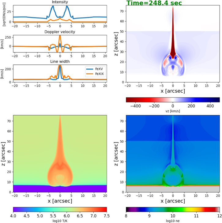
Figure 21. Snapshot of the Termination_shocks model (see Table 1 and Appendix A; Takasao et al. 2015) at t = 248 s. Top right: vertical component of plasma velocity (vz , negative/red is downflow) showing the sunward reconnection outflow. Bottom right: distribution of the free electron number density ne . Bottom left: temperature distribution. Top left: zeroth (line intensity), first (Doppler velocity; positive is redshift), and second (line width) moments of Fe xv 284 Å and Fe xix 108 Å lines, when observed along the − z-direction (i.e., top-down view). See Figure 16 for time evolution of the intensity and Doppler shifts.
Download figure:
Standard image High-resolution imageAppendix B: Synthesis of MUSE Spectral Observables from Models
The MUSE observables shown in the paper are synthesized from different models using the MUSE response functions. The MUSE spectral response functions provide the detector response across all 1024 spectral pixels for all three channels, per unit emission measure (1027 cm−5), at a specified slit (1–37), temperature, and Doppler velocity, as described in detail in De Pontieu et al. (2020). MHD models are first sampled as velocity–DEM distributions (Cheung et al. 2019) and then folded with the MUSE response functions to generate synthetic spectra. Here we focus on the main lines: Fe xix and Fe xxi 108 Å, Fe ix 171 Å, and Fe xv 284 Å. The response functions are computed using the latest CHIANTI database version and include instrumental effects (such as instrumental line broadening) and thermal broadening of the lines. The response functions calculate the predicted spectra in units of [DN s−1 pix−1], where the pixel is MUSE spectral raster pixel which has a sampling rate of 04 in the rastering (perpendicular to slits) direction, and a sampling of 0
167 along slits. For this paper, even when the synthetic images shown have a different sampling than a MUSE raster (e.g., MURaM simulations sampled at 192 km, equivalent to 0
265), we have opted to continue using the same response functions (and thus effective area) to demonstrate the count rate is sufficient for the relevant features.
Appendix C: Definition of Spectral Moments
In the paper, we show the zeroth (I0, aka line intensity), first (I1, aka Doppler velocity), and second (I2, aka total line width) moments of the MUSE synthetic observables from models, and they are defined, respectively, as follows:


where j is the index of the spectral bin, Fj is the intensity in spectral bin j in units of DN s−1 pix−1, and vj is the Doppler velocity in km s−1.