Abstract
The Fourier transformation is an effective and efficient operation of Gaussianization at the one-point level. Using a set of N-body simulation data, we verified that the one-point distribution functions of the dark matter momentum divergence and density fields closely follow complex Gaussian distributions. The one-point distribution function of the quotient of two complex Gaussian variables is introduced and studied. Statistical theories are then applied to model one-point statistics about the growth of individual Fourier modes of the dark matter density field, which can be obtained by the ratio of two Fourier-transformed cosmic fields. Our simulation results proved that the models based on the Gaussian approximation are impressively accurate, and our analysis revealed many interesting aspects of the growth of dark matter’s density fluctuation in Fourier space.
Original content from this work may be used under the terms of the Creative Commons Attribution 4.0 licence. Any further distribution of this work must maintain attribution to the author(s) and the title of the work, journal citation and DOI.
1. Introduction
Understanding the statistical properties of the inhomogeneity in the spatial distribution of dark matter and its evolution in an expanding universe is one of the most crucial subjects in cosmology. The growing process of density fluctuation is not simple, even for a system composed of collisionless dark matter particles solely. Complexities lie in many aspects. Statistically, though the primordial density fluctuation is assumed to be Gaussian or nearly so with possibly a small amount of primordial non-Gaussianity (see the review of Chen 2010, and references therein), the nonlinear gravitation evolution and other physical processes would drive the distribution of late-time dark matter to be highly non-Gaussian. Gaussian distribution is mathematically simple for practical application and can be fully described by its first two moments. However, the non-Gaussianity means that an entire hierarchy of higher-order cumulants or correlation functions is awaiting exploration. Furthermore, it has been shown that the distribution of dark matter is very close to the lognormal distribution and cannot be completely specified by its moments (Coles & Jones 1991; Carron 2011).
Non-Gaussianity makes measurement complex and difficult. If one intends to extract information from late-time density fields, statistics beyond the two-point level (Scoccimarro et al. 2001; Bernardeau et al. 2002; Sefusatti et al. 2006) are needed. In attempts to simplify the analysis, several Gaussianization schemes have been proposed and applied with notable success (e.g., Neyrinck et al. 2009; Scherrer et al. 2010; Yu et al. 2011; Carron & Szapudi 2013). The schemes really help reduce the non-Gaussianity and enhance the cosmological information in the two-point statistics (e.g., Yu et al. 2016; Repp & Szapudi 2018). The essence of Gaussianization is to perform a local transformation so that the non-Gaussianity in statistics of the transformed field at the first few low orders might be significantly suppressed. Then the Gaussian approximation could be applied to model the corresponding statistics. One has to keep in mind that non-Gaussianity never vanishes, but instead has a different appearance (Qin et al. 2020).
Matsubara (2007) formally derived that, for an arbitrary random field in a spatially homogeneous and sufficiently large space, the one-point probability distribution function (one-point PDF) of its Fourier mode shall approach Gaussian, provided that the polyspectra P(2n)( k ,…, k ; − k ,…, − k ) are finite for any positive integer n. For a cosmic density field, spatial homogeneity is normally ensured. The condition of finite polyspectra at arbitrary even orders has not been exhaustively verified. But non-Gaussianity in the density field on most scales with k ≠ 0 is believed to be finite, since the volume average correlation functions derived from cosmological simulations and galaxy surveys are always finite up to detected ranks (e.g., Bouchet & Hernquist 1992; Meiksin et al. 1992; Gaztañaga & Frieman 1994; Croton et al. 2004; Hellwing et al. 2010; Cappi et al. 2015). Actually, part of the conclusions of Matsubara (2007) have already been proved to be applicable to the cosmic density field in N-body simulations by Hikage et al. (2004).
Falck et al. (2021) recently measured the one-point PDFs of Fourier modes of the dark matter density fields of the Indra simulation suite. They found that the Gaussian approximation of Matsubara (2007) is consistent with simulations on scales as large as 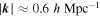 with relatively good accuracy. Another independent study by Qin et al. (2022) comprehensively tested the conclusions of Matsubara (2007) and validated that the Gaussian approximation can hold up to scales of
  for one-point PDFs of both modulus and phases. Therefore the density field in Fourier space poses very interesting statistical features. Its Fourier mode (even in the nonlinear regime) closely follows the Gaussian distribution, while the phase correlation of two points is already non-negligible, and the bispectrum and trispectrum are apparently significant (see also Matarrese et al. 1997; Scoccimarro 2000; Verde & Heavens 2001; Gualdi et al. 2021).
It appears that the Fourier transformation acts as a special type of Gaussianization, enabling us to understand the statistics of the cosmic density field in Fourier space at the one-point level. This work goes further and aims to apply the idea to model the particular type of statistics about the ratio of two different cosmic fields A and B in Fourier space, namely X k ≡ A k /B k .
The mode-dependent growth function of the dark matter density field utilized in Falck et al. (2021) falls into this category. In theory, the evolution of individual modes of the density field is intrinsically deterministic if actions other than gravitational force can be ignored (e.g., Sahni & Coles 1995; Bernardeau et al. 2002). However, the complicated effects of mode coupling will make the growth have a distribution over different modes. Using multiple realizations of their Indra simulation suits, Falck et al. (2021) characterize the growth of Fourier modes of the density field by defining the mode-dependent growth function as  . The Fourier-transformed density contrast δ
k
at a given redshift z and the initial redshift zi
of their simulation are used. They found that D
k
(z) is stochastic over different realizations, and its distribution becomes wider at later epochs and higher
. The Fourier-transformed density contrast δ
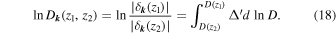
k
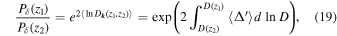
at a given redshift z and the initial redshift zi
of their simulation are used. They found that D
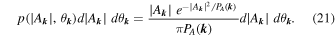
k
(z) is stochastic over different realizations, and its distribution becomes wider at later epochs and higher  . The medians of D
k
and the averages of
. The medians of D
k
and the averages of  were also shown on various scales and at different redshifts, but no analytical formulae are provided for the distribution and related statistics. Here, we will demonstrate that the analytical approximation to the one-point PDF of D
k
can be derived based on the results of Matsubara (2007).
were also shown on various scales and at different redshifts, but no analytical formulae are provided for the distribution and related statistics. Here, we will demonstrate that the analytical approximation to the one-point PDF of D
k
can be derived based on the results of Matsubara (2007).
In principle, the Fourier mode of any type of nonlinear cosmic field, including momentum divergence, shall also obey the theorem of Matsubara (2007), as long as prerequisite conditions are satisfied. Jennings & Jennings (2015) proposed a concept of stochastic growth rate to help develop perturbative theories of the redshift distortion effect, based on their numerical findings on the ratio of the velocity divergence field to the density field in Fourier space. This is another example of the ratio of cosmic fields in Fourier space, whose distribution could be examined and formulated. It is still challenging to conduct robust and accurate statistics of the volume-averaged velocity field from discrete samples deep into the nonlinear regime. Therefore, we instead consider using the momentum divergence field, since the momentum divergence could be easily measured from simulation (Pan 2020).
As will be shown later, for dark matter, the quotient of momentum divergence to density is a direct measure of the growth rate of the density field at any given moment z and scale  . Thus, the mode growth rate defined in this way could be linked to the mode-dependent growth function D
k
(z). But unlike the stochastic growth rate in Jennings & Jennings (2015), it could not be directly used for the redshift distortion effect.
. Thus, the mode growth rate defined in this way could be linked to the mode-dependent growth function D
k
(z). But unlike the stochastic growth rate in Jennings & Jennings (2015), it could not be directly used for the redshift distortion effect.
The entire paper is structured as follows. The definition and theoretical foundation are laid mainly in Section 2, which is then compared with the simulation data in Section 3. Section 4 is about the performance test of empirical models for the mean mode growth rate. This study ends with a summary and discussion in the last section.
2. Theories on Statistics of Quotient of Two Complex Gaussian Random Variables
Starting from a more general expression of the distribution of two complex Gaussians, we summarize the major mathematical background. The results are then extended with two particular statistics, namely, the mode-dependent growth function and the mode growth rate. Their statistical meanings are stated and will be investigated in the following part of this work.
2.1. Distribution of the Ratio of Two Complex Gaussians
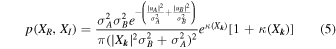
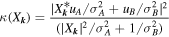
Without loss of generality, A k and B k are supposed counterparts in the Fourier space of two random fields A and B of any kind, then X k is defined as the quotient of the two complex random variables, X k = A k /B k . Calculating the distribution of X k requires complete knowledge of the joint distribution of A k and B k . Practically, the closed-form analytical expression is intractable, except for a few cases. Fortunately, if A k and B k are both distributed as Gaussian, analytical formulae exist in the literature, which we reproduce here as the basis of our work.
Let ![${\boldsymbol{q}}={[{A}_{{\boldsymbol{k}}},{B}_{{\boldsymbol{k}}}]}^{T}$](https://content.cld.iop.org/journals/0004-637X/933/1/24/revision1/apjac6fddieqn7.gif) be a 2 × 1 complex Gaussian random vector, there are the mean of the vector
be a 2 × 1 complex Gaussian random vector, there are the mean of the vector ![${\boldsymbol{u}}=\left\langle {\boldsymbol{q}}\right\rangle ={[{u}_{A},{u}_{B}]}^{T}$](https://content.cld.iop.org/journals/0004-637X/933/1/24/revision1/apjac6fddieqn8.gif) and the covariance matrix
and the covariance matrix
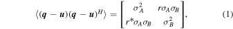
 means the average, (…)* is the conjugate, (…)T
and (…)H
refer to the transpose and conjugate transpose, respectively, and r is the parameter of the correlation coefficient. Let X
k
= A
k
/B
k
= XR
+ iXI
, Li & He (2019) derive that the joint PDF of XR
and XI
can be written as
means the average, (…)* is the conjugate, (…)T
and (…)H
refer to the transpose and conjugate transpose, respectively, and r is the parameter of the correlation coefficient. Let X
k
= A
k
/B
k
= XR
+ iXI
, Li & He (2019) derive that the joint PDF of XR
and XI
can be written as
in which
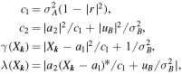
with a1 = r σA /σB and a2 = uA − a1 uB . Note that the formula is general and is not restricted to the case of independently distributed A k and B k .
The mean of X k , if uB ≠ 0, is given by

and if uB = 0

while higher-order moments  do not exist unless
  (Wu 2019; Li & He 2019).
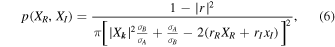
If A k and B k are independent, then r = 0 and the joint PDF reduces to
with
(e.g., Pham-Gia et al. 2006; Nadimi et al. 2018).
A more special case is uA = uB = 0, the joint PDF is in the form of
in which r = rR + irI (Baxley et al. 2010). At this stage, we have derived the main equation, which will be extended to two particular statistics in the context of structure formation in the following part of this study.
2.2. The Mode-dependent Growth Function
For generality, we slightly extended the notion of Falck et al. (2021), by defining a complex mode-dependent growth function  ,
,

where δ
k
(z) is the Fourier counterpart of the dimensionless density contrast  at redshift z, with ρ denoting the density and z2 > z1. If we denote
 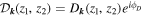 , the amplitude
  is commonly used and is the target function that we want to analyze. As formerly mentioned in Section 1, the nonlinear field of δ
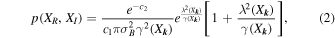
k
(z) in the Fourier space could be approximately treated as Gaussian distributed. This generally guarantees the usage of Equation (2) to model p(D
k
, ϕD
).
is commonly used and is the target function that we want to analyze. As formerly mentioned in Section 1, the nonlinear field of δ
k
(z) in the Fourier space could be approximately treated as Gaussian distributed. This generally guarantees the usage of Equation (2) to model p(D
k
, ϕD
).
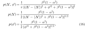
Let the density power spectrum at z be  , and let the density cross-spectrum at two different redshifts be
  . With the consideration that the density field is statistically isotropic and homogeneous, δ
k
satisfies
. With the consideration that the density field is statistically isotropic and homogeneous, δ
k
satisfies  and
and  . This exactly corresponds to the case of Equation (6), but with the correlation coefficient
  and rI
= 0. If we further let
and rI
= 0. If we further let  , Equation (6) proceeds to another form
with r < 1 and −π ≤ ϕD < π.
With the results of Section 2.1, we could derive the mean  and the median D
k
,1/2 = t. What is important is that we have identified the meanings of two often used quantities. The first is that
and the median D
k
,1/2 = t. What is important is that we have identified the meanings of two often used quantities. The first is that  is the mean of the complex mode-dependent growth function
  the second is that
  is the median value of Dk
.
is the median value of Dk
.
Unfortunately, the mean  does not have a simple analytic form and could only be calculated with numerical integration. In real applications, one could always numerically compute an averaged D
k
over many simulation realizations. However, the mean value of the logarithm of D
k
used in Falck et al. (2021),
does not have a simple analytic form and could only be calculated with numerical integration. In real applications, one could always numerically compute an averaged D
k
over many simulation realizations. However, the mean value of the logarithm of D
k
used in Falck et al. (2021),  , exists. Under the Gaussian approximation,
  obeys the dubbed log-Rayleigh distribution, in which the expectation is

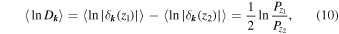
where C is the Euler constant defined by 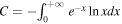 (Rivet et al. 2007). Subsequently,
  could be related to the density power spectrum as
which can be used straightforwardly to interpret the results of Falck et al. (2021).
2.3. A Minor Note about Possible Applications to Bias
If we go beyond the dark matter density field by considering the density field of biased tracers in the Fourier space δg
(
k
), which has a complex bias function as  relative to dark matter δm
(
k
), mathematical results in Section 2.2 can be essentially adopted after the replacements of δ
k
(z1) → δg
(
k
) and δ
k
(z2) → δm
(
k
). Therefore, the ordinary bias function
relative to dark matter δm
(
k
), mathematical results in Section 2.2 can be essentially adopted after the replacements of δ
k
(z1) → δg
(
k
) and δ
k
(z2) → δm
(
k
). Therefore, the ordinary bias function 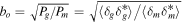 is the median value of
  . While another commonly cited bias function
 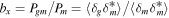 is the average of
  , with denoting
  as the cross-spectrum of the two fields. The difference between bo
and bx
vanishes in the limit of
as the cross-spectrum of the two fields. The difference between bo
and bx
vanishes in the limit of  , that is the case when bias shows little stochasticity.
The number density of biased traces such as halos and galaxies is usually much lower than that of dark matter in simulations. Understanding and devising methods to suppress discreteness effects on δg ( k ) is not an easy task. Therefore, we will leave further exploration of biased density fields for future research and concentrate on the distribution of dark matter only.
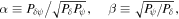
2.4. The Mode Growth Rate
In analogy with Jennings & Jennings (2015), we start from the continuity equation, which is valid for dark matter as long as dark matter does not annihilate significantly,

in which a = 1/(1 + z) with z being the redshift corresponding to cosmic time τ, δ is the dark matter density contrast at position r , and v labels the peculiar velocity. In Fourier space, it turns out to be

in which ψ
k
(shorthand for ψ(
k
)) is the Fourier transform of the momentum divergence ![$\psi ({\bf{r}})\equiv -{\rm{\nabla }}\cdot \left[(1+\delta ){\boldsymbol{v}}({\bf{r}})\right]/{Haf}$](https://content.cld.iop.org/journals/0004-637X/933/1/24/revision1/apjac6fddieqn38.gif) , where H is the Hubble parameter, and
, where H is the Hubble parameter, and  is the linear growth rate defined with respect to the linear growth function D. Unlike D
k
, the linear growth function is scale-independent and is defined as the amplitude factor of the density contrast δ relative to that at the present time.
is the linear growth rate defined with respect to the linear growth function D. Unlike D
k
, the linear growth function is scale-independent and is defined as the amplitude factor of the density contrast δ relative to that at the present time.
On the other hand, if we denote  , then
of which the real part is only about the growth of the moduli and the imaginary component is solely about phases. Let X k ≡ ψ k /δ k , combining Equation (12) with Equation (13) yields the following,

 and
and  refer to the real and imaginary parts of X
k
, respectively,
refer to the real and imaginary parts of X
k
, respectively,

Here, a is replaced by the linear growth function D as the time variable.
It is apparent that X
k
effectively becomes the mode growth rate of dark matter’s density field, of which  is the mode’s amplitude growth rate and
  stands for the mode’s phase growth rate. In the linear regime ψ
k
= δ
k
,
stands for the mode’s phase growth rate. In the linear regime ψ
k
= δ
k
,  and
and  , the amplitudes will grow linearly with D while the phases will remain invariant. However, when gravitational nonlinearity increases, ψ
k
≠ δ
k
, it is expected that stochasticity in
, the amplitudes will grow linearly with D while the phases will remain invariant. However, when gravitational nonlinearity increases, ψ
k
≠ δ
k
, it is expected that stochasticity in  and
and  will become stronger due to the effects of mode coupling and multistreaming.
The exact modeling of the distribution of X
k
requires complete knowledge of the joint distribution of δ
k
and ψ
k
. Again, based on the results of Matsubara (2007), if ψ
k
closely follows the Gaussian distribution in a similar way as δ
k
does, then the results of Section 2.1 can be used to model  .
.
Since  , after denoting

and
the one-point PDFs of X
k
,  and
and  can be derived from Equation (6) without difficulty,
both  and
and  are actually the Student’s t-distribution with 2 degrees of freedom.
A nice property of defining the mode growth rate with Equation (15) is that the first-order moment  is well determined,

In fact, Equation (17) also points out that  can be estimated by the ratio of two nonzero power spectra, free of the possible numerical catastrophe when
  .
.
2.5. Links Among Mode-dependent Growth Function, Mode Growth Rate, and Power Spectrum
The amplitude of the mode-dependent growth function at redshift z1 with respect to z2 (z2 > z1) could actually be related to  through
Taking the average in the Gaussian ansatz then leads to
or

This means that  is a measure of the logarithmic growth rate of the nonlinear density power spectrum, as long as the Gaussian approximation to δ
k
and ψ
k
holds its effectiveness.
is a measure of the logarithmic growth rate of the nonlinear density power spectrum, as long as the Gaussian approximation to δ
k
and ψ
k
holds its effectiveness.
3. Comparison with N-body Simulation
In Section 2, the analytical expressions of the distributions of the mode-dependent growth function and the mode growth rate are derived under the assumption that the density field δ k and the momentum divergence field ψ k follow the Gaussian distribution. In this section, simulation data are used to examine whether the prerequisite conditions are met, and then the analytical formulas of two statistics are compared.
3.1. The Simulation and Numerical Issues
In this work, the Pangu simulation in Li et al. (2012) is recruited. The dark matter-only simulation is conducted with a memory-optimized version of GADGET2 (Springel 2005). The cosmological parameters are Ωm = 0.26, Ωb = 0.044, ΩΛ =0.74, h = 0.71, and σ8 = 0.8. The simulation uses N = 30723 dark matter particles in a cubic periodic box with L = 1 h−1 Gpc on one side. Each particle has a mass of 2.48915 × 10⁹ h−1 M⊙ and the Plummer-equivalent force softening length is 7 h−1 kpc. The simulation starts from an initial redshift of z = 127. Since we are mainly interested in regimes with considerably developed non-Gaussianity, about 13 snapshots at redshifts from z = 2 to 0 are selected. The mass resolution of the simulation supports accurate measurement of power spectrum at scales 1 < k ≲ 10 h Mpc−1, meanwhile its box size can provide sufficient numbers of modes at large scales k < 0.1 h Mpc−1 and makes the systematics in modes of short wavelengths induced by the absence of long-wavelength modes negligible (e.g., Crocce & Scoccimarro 2006; Takahashi et al. 2008).
The numerical fast Fourier transformation (FFT) is implemented with the FFTW3 package (Frigo & Johnson 2005). To obtain accurate measurements of Fourier modes of density, momentum divergence, and related power spectra, the prescription of Yang et al. (2009) and Pan (2020) is adopted to compensate for the effects of aliasing and smoothing. The third-order orthogonalized Battle-Lemarié spline function is used when assigning dark matter particles to FFT grids. But aliasing cannot be completely removed, and numerical experiments indicate that if 1% precision is required, it is safe to use Fourier modes on scales k < 0.67 kN (Appendix A), where kN is the Nyquist frequency.
The quality of the numerical measurement is further controlled by applying criteria based on shot noise. We restrict our exploration to the scale range within which the influence of the power spectrum of the shot noise is less than 1%. Additionally, the number of FFT grids is set by the requirement that the mean number of particles in a grid cell should be greater than one. Therefore, the largest number of FFT grids used in this work is 20483. By applying these conservative rules, the influence of discreteness becomes minuscule; henceforth, we do not make any shot noise correction unless specified otherwise.
The last point we want to address here is that in this work only one simulation realization is used. Thus, the ergodicity principle is assumed when comparing simulations with theories. Specifically, statistics computed with all modes identical to  from a single simulation are considered statistically equivalent to statistics of the mode at
k
over many realizations, with some reasonable fluctuations attributed to cosmic variance.
from a single simulation are considered statistically equivalent to statistics of the mode at
k
over many realizations, with some reasonable fluctuations attributed to cosmic variance.
3.2. One-point PDFs of δk and ψk
If a complex random variable  is Gaussian distributed with zero mean and variance
  , its modulus
  will follow a Rayleigh distribution, and its phase θ
k
will be uniformly distributed,
will follow a Rayleigh distribution, and its phase θ
k
will be uniformly distributed,
The z = 0 snapshot of the Pangu simulation, which has the strongest non-Gaussianity, is used to check the goodness of Gaussian approximation. The measured PDFs of δ k and ψ k together with predictions by Equation (21) in six k bins (Table 1) are shown in Figure 1, the agreement of the Gaussian model with the simulation is obvious. To quantify the deviations from Gaussianity, the skewness and kurtosis of the real and imaginary parts of δ k and ψ k are calculated and shown in Figure 2.
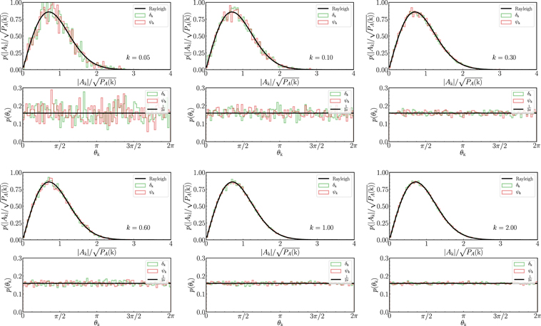
Figure 1. One-point PDFs of δ k and ψ k of dark matter in the z = 0 snapshot of the Pangu simulation. The results are shown in six k bins (Table 1). The symbol A in the plot represents δ or ψ accordingly. Black solid lines are predicted by Equation (21) with Pδ ( k ) and Pψ ( k ) estimated from the simulation.
Download figure:
Standard image High-resolution image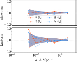
Figure 2. Skewness and kurtosis of the real and imaginary parts of δ k and ψ k . Filled circles connected with solid lines are about the real parts, and filled triangles linked with dashed lines are of the imaginary parts. For perfect Gaussian distribution, skewness and kurtosis are zeros as denoted by those horizontal black dashed lines. The blue and orange bands are the 1σ scatters estimated from 1000 Gaussian realizations in each k bin. Only the real parts of δ k and ψ k are shown for clearness. The shaded area at the right end is the regime where k > 0.67 kN .
Download figure:
Standard image High-resolution imageTable 1. k Bin Centers and their Widths Selected to Calculate Distribution Functions
| k | Δk | Nmode |
|---|---|---|
| 0.05 | 0.01 | 1431 |
| 0.10 | 0.01 | 5299 |
| 0.30 | 0.005 | 23246 |
| 0.60 | 0.001 | 18929 |
| 1.00 | 0.001 | 51089 |
| 2.00 | 0.0005 | 99448 |
Note. The number of modes Nmode are counted within k ± Δk.
Download table as: ASCIITypeset image
As expected, across wide scale ranges from quasi-linear to strongly nonlinear regime, skewness and kurtosis are consistent with a Gaussian distribution. To demonstrate the contribution of finite mode numbers to the skewness and kurtosis, in each k bin, we generate 1000 random Gaussian realizations. The sample size and the Gaussian parameters of each realization are kept the same as the simulation results. Then the skewness and kurtosis are extracted for each realization, and the mean and 1σ scatter of them are estimated. To reduce redundancy, only the results for the real parts of δ k and ψ k are presented in Figure 2, shown as blue and orange bands. The non-Gaussianity in one-point PDFs of δ k and ψ k seems to be hardly associated with the strength of nonlinearity.
Consequently, the conclusion is that the one-point distributions of δ k and ψ k can be modeled by Equation (21) remarkably well, even though the density field is highly non-Gaussian due to gravitational instability (Feldman et al. 2001; Sefusatti et al. 2006). The results of the density field are also consistent with those of Falck et al. (2021) and Qin et al. (2022). What is new and of great importance is that, for the first time, the momentum divergence field of dark matter is verified to be highly Gaussianized at a one-point level after the Fourier transformation. This extends the effectiveness of the results of Matsubara (2007) and practically fulfills a crucial prerequisite condition for applying the theories in Section 2.4 to model the mode growth rate.
3.3. Distribution of Mode-dependent Growth Function
The one-point PDFs of  , D
k
and ϕD
in the selected k bins are demonstrated in Figure 3. The plot is generated by comparing the z = 0 snapshot to the one at z = 2 of the Pangu simulation, together with the theoretical predictions of Equation (8). The contours of p(D
k
, ϕD
) measured from the simulation are noisy, but p(D
k
) and p(ϕD
) appear to be highly consistent with the predictions of the model in all scale bins.
, D
k
and ϕD
in the selected k bins are demonstrated in Figure 3. The plot is generated by comparing the z = 0 snapshot to the one at z = 2 of the Pangu simulation, together with the theoretical predictions of Equation (8). The contours of p(D
k
, ϕD
) measured from the simulation are noisy, but p(D
k
) and p(ϕD
) appear to be highly consistent with the predictions of the model in all scale bins.
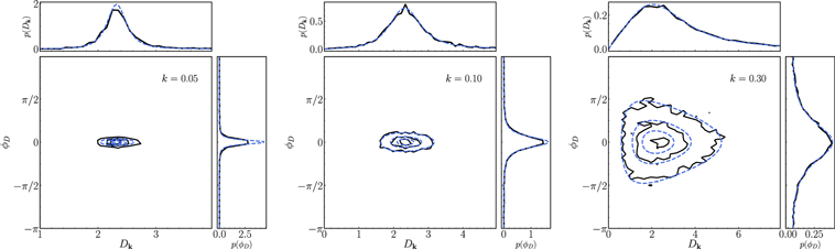
Figure 3.
p(D
k
, ϕD
) in the six k bins as specified in Table 1. The mode-dependent growth function  in this plot is z1 = 0 and z2 = 2. In each panel, contour lines mark the levels at 20%, 50%, and 80% of the maximum value of the distribution, p(D
k
, ϕD
) is then integrated along each dimension to produce p(D
k
) and p(ϕD
) which are drawn in attached side subplots. The simulation results are colored with black solid lines, and the analytical models (Equation (8)) are plotted in blue dashed lines.
in this plot is z1 = 0 and z2 = 2. In each panel, contour lines mark the levels at 20%, 50%, and 80% of the maximum value of the distribution, p(D
k
, ϕD
) is then integrated along each dimension to produce p(D
k
) and p(ϕD
) which are drawn in attached side subplots. The simulation results are colored with black solid lines, and the analytical models (Equation (8)) are plotted in blue dashed lines.  and
and  as inputs to the models are estimated from the simulation.
Download figure:
Standard image High-resolution imageFor large-scale modes (k = 0.05 h Mpc−1), widths of the distributions p(D k ) and p(ϕD ) are apparently narrow, indicating that the deviation from linear evolution is mild. With increasing k, the distributions become much wider, p(ϕD ) tends to become uniformly distributed, and p(D k ) becomes skewed with a long tail. It implies that with the information provided by one-point statistics of the density field alone, one can hardly recover the cosmic density field exactly at earlier times in the nonlinear regime.
3.4. Distribution of Mode Growth Rate
Figure 4 shows the one-point PDFs of  in selected k bins calculated from the simulation data, together with the predictions of Equation (16). The measurements can be well approximated by the model based on the Gaussian assumption.
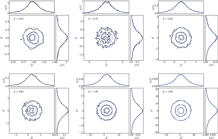
Figure 4. Similar to Figure 3, but for  .
.  and
and  , produced by integrating
  , are shown in the side subplots attached to each panel. Analytical models (Equation (16)) are plotted in blue dashed lines. Again,
  ,
,  , α and β as input parameters to the models are taken from the simulation results.
Download figure:
Standard image High-resolution imageSince  and
and  are following the Student’s t-distribution with 2 degrees of freedom, their second-order moments do not exist, and the standard deviations numerically computed from the simulation data are meaningless. By Equation (16), we propose taking an alternative quantity,
  , as an appropriate function to characterize the width of
  . As shown in Figure 5 without surprise, the widths of
  become larger with increasing nonlinearity (from z = 2 to z = 0). If we further decompose the momentum divergence into two independent components, ψ = ψs
+ ψδ
, with ψs
the stochastic part uncorrelated with density at all, and ψδ
the part fully correlated with the density field that can be expressed as ψδ
(
k
) = Tδ→ψ
(
k
)δ(
k
) with a certain transfer function Tδ→ψ
in Fourier space. If one denotes the power spectrum of ψs
as
become larger with increasing nonlinearity (from z = 2 to z = 0). If we further decompose the momentum divergence into two independent components, ψ = ψs
+ ψδ
, with ψs
the stochastic part uncorrelated with density at all, and ψδ
the part fully correlated with the density field that can be expressed as ψδ
(
k
) = Tδ→ψ
(
k
)δ(
k
) with a certain transfer function Tδ→ψ
in Fourier space. If one denotes the power spectrum of ψs
as  , it leads to

From this decomposition, it turns out that the distribution widths of  are mainly caused by the stochastic part of the momentum divergence ψs
.
are mainly caused by the stochastic part of the momentum divergence ψs
.
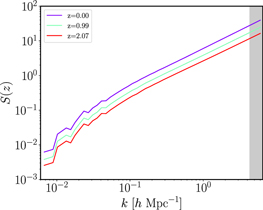
Figure 5. Characteristic width parameter 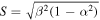 of the one-point distribution
  as a function of scales.
Download figure:
Standard image High-resolution imageIt is interesting to note that there is a crude scaling relation S(z) ∝ D(z) whose accuracy is better than 10% within wide ranges of scale and redshift (Figure 6). A deviation greater than 5% occurs mainly on scales 0.1 ≲ k ≲ 1 h Mpc−1 for z > 1. By the one-loop Eulerian perturbation theory, S scales with D in the weakly nonlinear regime (e.g., Smith et al. 2009; Pan 2020). But in the nonlinear regime, where the one-loop theory breaks seriously, the scaling relation still holds valid with considerable precision, and the performance turns out to be even better at lower redshifts, which is really intriguing. However, it is necessary to be cautious when quoting the precision of the scaling relation for k < 0.1 h Mpc−1, S(z) is sensitive to the treatment of shot noise in the weakly nonlinear regime (see Appendix B for more details).
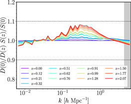
Figure 6. [S(z)/D(z)]/[S(0)/D(0)] measured at multiple redshifts 0 ≤ z ≲ 2. The shaded regime is where k > 0.67 kN . Here, the shot noise in the power spectra used to compute S is not subtracted.
Download figure:
Standard image High-resolution imageSince the symmetry of ![$\left[\delta (-{\boldsymbol{k}}),\psi (-{\boldsymbol{k}})\right]=\left[{\delta }^{* }({\boldsymbol{k}}),{\psi }^{* }({\boldsymbol{k}})\right]$](https://content.cld.iop.org/journals/0004-637X/933/1/24/revision1/apjac6fddieqn84.gif) has ensured
has ensured  ,
,  is then of major interest. As already mentioned in Equation (17),
  is equal to
  . This means that Pδ
ψ
/Pδ
is a good estimator of
. This means that Pδ
ψ
/Pδ
is a good estimator of  . In Figure 7, we demonstrate the effectiveness of Equation (17) with simulation data. The mean differences between Pδ
ψ
/Pδ
and
. In Figure 7, we demonstrate the effectiveness of Equation (17) with simulation data. The mean differences between Pδ
ψ
/Pδ
and  are generally less than 1% within the scale 0.007 ≲ k ≲ 6 h Mpc−1.
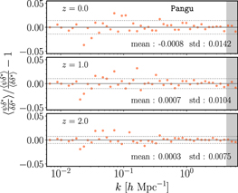
Figure 7. Relative differences between Pδ
ψ
/Pδ
and  . Data from three snapshots at z = 0, 1, 2 of the Pangu simulation are used. Horizontal solid lines represent the mean of the differences, and dashed lines delimit the standard deviations. In each subplot, the means and standard deviations are calculated from all data points along with k scales. The gray shaded area marks the regime where k > 0.67 kN
.
. Data from three snapshots at z = 0, 1, 2 of the Pangu simulation are used. Horizontal solid lines represent the mean of the differences, and dashed lines delimit the standard deviations. In each subplot, the means and standard deviations are calculated from all data points along with k scales. The gray shaded area marks the regime where k > 0.67 kN
.
Download figure:
Standard image High-resolution image3.5. The Mean Mode Growth Rate in Simulation
The mean mode growth rate  is measured from the simulation data using Pδ
ψ
/Pδ
. Its dependence on multiple redshifts and scales is fully investigated and shown in Figure 8. On large scales k ≲ 0.1 h Mpc−1,
is measured from the simulation data using Pδ
ψ
/Pδ
. Its dependence on multiple redshifts and scales is fully investigated and shown in Figure 8. On large scales k ≲ 0.1 h Mpc−1,  at all redshifts, which is consistent with the linear theory for gravitational evolution. In the intermediate nonlinear regime,
  rises with increasing k, and is systematically greater when the redshift approaches zero. The value of
  has a single peak positioned between 1 ∼ 4 h Mpc−1, and the peak height is less than 2. The general trend is that the peaks of
  at higher redshifts are located at larger k than those at lower redshifts, but the relations among peak position, peak height, and redshift are not simple.
Figure 8. Mean mode growth rates  estimated from the simulation by Pδ
ψ
/Pδ
, as functions of scales (left panel) and redshifts (right panel). Lines of various colors label
estimated from the simulation by Pδ
ψ
/Pδ
, as functions of scales (left panel) and redshifts (right panel). Lines of various colors label  of different redshifts (left panel) and scales (right panel) accordingly. Again, the gray region in the left panel is k > 0.67 kN
.
of different redshifts (left panel) and scales (right panel) accordingly. Again, the gray region in the left panel is k > 0.67 kN
.
Download figure:
Standard image High-resolution imageThe scale dependence of  is shown in the right panel of Figure 8. In general, the amplitude of
  along the redshift is stronger for higher k, but
  at k ≳ 1 h Mpc−1 tends to decrease when z → 0, contrary to its behavior at k ≲ 1 h Mpc−1. In addition, nontrivial oscillatory structures are also found at k ≳ 1 h Mpc−1. The origins of these phenomena are still unclear. The measurement is based on only one simulation realization and could be camouflaged by cosmic variance.
10
One potential solution is to have a large number of simulation realizations with ∼ h−3 Gpc3 volume and mass resolution better than ∼ 109
h−1
M⊙. This is a prerequisite for relevant investigation toward smaller scales, probably to k ∼ 10 h Mpc−1. We leave this for further work.
at k ≳ 1 h Mpc−1 tends to decrease when z → 0, contrary to its behavior at k ≲ 1 h Mpc−1. In addition, nontrivial oscillatory structures are also found at k ≳ 1 h Mpc−1. The origins of these phenomena are still unclear. The measurement is based on only one simulation realization and could be camouflaged by cosmic variance.
10
One potential solution is to have a large number of simulation realizations with ∼ h−3 Gpc3 volume and mass resolution better than ∼ 109
h−1
M⊙. This is a prerequisite for relevant investigation toward smaller scales, probably to k ∼ 10 h Mpc−1. We leave this for further work.
4. Empirical Models for the Mean Mode Growth Rate in Nonlinear Regime
4.1. Fitting Formulae
Developing theoretical models of  in the strongly nonlinear regime from first principles is a difficult task, desperately in demand of ingenious ideas. Therefore, we turn to building templates for nonlinear
  empirically in different cosmologies. The solution is already provided by Equation (20), together with the algorithm based on the first-order finite difference method. We first pick up a fitting formula for Pδ
and construct a table as a function of redshift z, with a fine increment of Δz. Then
empirically in different cosmologies. The solution is already provided by Equation (20), together with the algorithm based on the first-order finite difference method. We first pick up a fitting formula for Pδ
and construct a table as a function of redshift z, with a fine increment of Δz. Then  at a given redshift z is calculated numerically with the derivative

where  , z ± Δz are two interpolation boundaries that enclose z in the constructed Pδ
table. We have tried different values of Δz and
, z ± Δz are two interpolation boundaries that enclose z in the constructed Pδ
table. We have tried different values of Δz and  , and once the result becomes stable as
  , we take it as a phenomenological model of
  .
.
In this work, emulators of HMCODE 2020 (Mead et al. 2021), EUCLID EMU (version 2; Euclid Collaboration et al. 2020), BACCO EMU (Angulo et al. 2020), MIRA TITAN (Lawrence et al. 2017), and the empirical model of Takahashi 2012 (Takahashi et al. 2012) are chosen to generate the nonlinear power spectrum. In Figure 9, the performance of these prescriptions is presented in comparison to the simulation results. These fitting formulae do recover the power spectrum very well, but cannot accurately reproduce  in the strongly nonlinear regime, for example, k ≳ 1 h Mpc−1 for all shown cases. Again, the results presented are of a single simulation set and more realizations are needed to draw reliable conclusions. Nevertheless, one thing is certain: it seems
  can be a useful tool for distinguishing the performance of different fitting formulae of the power spectrum in the strongly nonlinear regime.
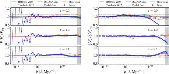
Figure 9. Comparison between simulations and empirical models, in terms of the power spectrum (left panel) and  (right panel). Solid lines of different colors are given by fitting formulae as specified on the top of each panel, square points connected with blue lines are measurements of simulations, and dashed horizontal lines are used to mark the ±5% differences. The shaded regions are where k > 0.67 kN
. The reference template (quantity with subscript “ref”) is given by HMCODE 2020 (Mead et al. 2021).
(right panel). Solid lines of different colors are given by fitting formulae as specified on the top of each panel, square points connected with blue lines are measurements of simulations, and dashed horizontal lines are used to mark the ±5% differences. The shaded regions are where k > 0.67 kN
. The reference template (quantity with subscript “ref”) is given by HMCODE 2020 (Mead et al. 2021).
Download figure:
Standard image High-resolution image4.2. Scale Transformation
It is well known that the nonlinear dimensionless power spectrum of the dark matter density field, Δ2(k) = P(k)k3/(2π2), can be approximated as a function of the linear dimensionless power spectrum  after a scale transformation,

The scaling ansatz was first proposed to model the two-point correlation function by Hamilton et al. (1991), then developed in the Fourier space by Peacock & Dodds (1994). It is found that Equation (24) could also be applied to approximately recover the bispectrum when nonlinearity is not strong (Pan et al. 2007). Along with Equation (20), we conjecture that the transformation of Equation (24) could help to understand  .
.
The two formulae of HMCode 2020 and Takahashi 2012 are called to facilitate our experiment. The results of the simulation Pangu simulation and the two models are shown in Figure 10. It turns out that the scale transformation of Equation (24) is really useful, although an extra factor is needed in practice. For  , the mean mode growth rates at different epochs can be written as

rather than ![$F[{{\rm{\Delta }}}_{L}^{2}]$](https://content.cld.iop.org/journals/0004-637X/933/1/24/revision1/apjac6fddieqn116.gif) as one might naively expect. Here, F[…] refers to a general function of a certain form that may contain additional dependencies on the cosmological parameters, and the accuracy is better than 5%.
as one might naively expect. Here, F[…] refers to a general function of a certain form that may contain additional dependencies on the cosmological parameters, and the accuracy is better than 5%.
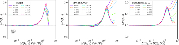
Figure 10. The mean mode growth rates as functions of  , kL
are given by Equation (24). The left panel shows the results computed from the Pangu simulation, and the middle and right panels are the results of the emulator HMCODE 2020 (Mead et al. 2021) and the empirical model Takahashi 2012 (Takahashi et al. 2012) accordingly with the same cosmology.
, kL
are given by Equation (24). The left panel shows the results computed from the Pangu simulation, and the middle and right panels are the results of the emulator HMCODE 2020 (Mead et al. 2021) and the empirical model Takahashi 2012 (Takahashi et al. 2012) accordingly with the same cosmology.
Download figure:
Standard image High-resolution imageThe peaks of  of the simulation and the two empirical models are basically relocated to a narrow range of
  after the scale transformation. But the differences between the simulation and the empirical models are still very prominent for
  . Empirical models of HMCode 2020 and Takahashi 2012 (the middle and right panels of Figure 10) produce rising tails on scales greater than peak locations, and these tails arise systematically higher at lower redshifts, which are not present in the Pangu simulation. Considering that empirical models are obtained through extensive calibration against simulations, the evolution of dark matter clustering in very strongly nonlinear regimes may be sensitive to numerical details of different simulations. One needs to be careful when using fitting formulae as templates if their
  goes beyond 1.3.
5. Summary
In this study, we demonstrate that nonlinear cosmic fields such as the dark matter density δ and the momentum divergence ψ can be effectively and efficiently Gaussianized by the Fourier transformation at the one-point level, which is an extension of the work of Matsubara (2007). Gaussianity of the one-point distributions of Fourier modes greatly simplifies analysis of the spatial distribution of dark matter and its evolution, as what has been shown in this work about functions given by the ratio of two complex random variables.
Analytical formulae about the one-point PDF of the quotient of two correlated complex Gaussian random variables are introduced and then applied to explore the statistical properties of two quantities used to describe the clustering evolution of dark matter. The first is the complex mode-dependent growth function  , defined as the ratio of δ
k
at two different epochs, X
k
= δ
k
(z1)/δ
k
(z2). The explicit model of the one-point PDF of
, defined as the ratio of δ
k
at two different epochs, X
k
= δ
k
(z1)/δ
k
(z2). The explicit model of the one-point PDF of  is in good agreement with the results of the N-body simulation. The amplitude of the complex mode-dependent growth function Dk
and its logarithm are also investigated. It is really intriguing that, for the dark matter density, the ratio of the cross-power spectrum to the auto-power spectrum and the ratio of the two auto-power spectra have particular statistical meanings. The former one is the mean of
is in good agreement with the results of the N-body simulation. The amplitude of the complex mode-dependent growth function Dk
and its logarithm are also investigated. It is really intriguing that, for the dark matter density, the ratio of the cross-power spectrum to the auto-power spectrum and the ratio of the two auto-power spectra have particular statistical meanings. The former one is the mean of  , while the square root of the latter is the median of the amplitude Dk
.
, while the square root of the latter is the median of the amplitude Dk
.
Another instance studied in this work is the complex mode growth rate, which is defined in Fourier space by the ratio  . With the continuity equation, we identify that the real part of X
k
,
. With the continuity equation, we identify that the real part of X
k
,  is the growth rate of the amplitude of the density mode, while the imaginary part
  relates to the phase growth rate. The Gaussian approximation to the one-point PDF
  is again developed and confirmed by simulation with good accuracy. It turns out that the mode’s amplitude growth rate
  and the mode’s phase growth rate
  both follow the Student’s t-distribution with 2 degrees of freedom. The distribution could be characterized by an alternative width parameter S, which increases with the strength of nonlinearity, and has an approximate scaling relation S ∝ D among different epochs.
As  is always zero, the information about the nonlinear evolution process of the density field in X
k
is mainly packed in the mean mode growth rate
is always zero, the information about the nonlinear evolution process of the density field in X
k
is mainly packed in the mean mode growth rate  . On large scales where nonlinearity is very weak,
  at all redshifts. When goes to the nonlinear regime, the increasing nonlinearity will drive
  away from unity. We further show that empirical formulae and theoretical models of the density power spectrum can provide satisfactory templates for
  in the weakly and intermediate nonlinear regime, but the agreement begins to drop drastically in the strongly nonlinear regime. The phenomenon becomes even more apparent after applying a scale transformation.
In summary, with the Gaussian approximation to cosmic fields in Fourier space, the statistical properties of the quotient of two complex Gaussian variables provide a novel approach to measuring the growth of individual modes of the dark matter density field. It has been proven to be very useful and can be readily applied in other large-scale structure studies with similar types of quantities. The results presented here emphasize the simplicity of the analysis in Fourier space and are worthy of more attention for further studies of cosmic structure formations.
Ming Li acknowledges support from the NSFC grants Nos. 11988101 and 12033008. Jun Pan acknowledges support from the NSFC grants of No. 11573030. Pengjie Zhang acknowledges support from the NSFC grant No. 11621303. Longlong Feng acknowledges support from the NSFC grant No. 11733010. Guoliang Li thanks the support from NSFC grant No. U1931210. Weipeng Lin thanks the NFSC grant No. 12073089. Haihui Wang is supported by the Shandong MSTI Project (2019JZZY010122) and the MIIT grant (J2019-I-0001).
The authors thankfully acknowledge computing and storage support from the cosmology simulation database (CSD) in the National Basic Science Data Center (NBSDC) and its fund NBSDC-DB-10, No. 2020000088.
We would like to thank the anonymous referee for helping us improve this work with their constructive comments.
Appendix A: Aliasing
In the ratio of Pδ
ψ
/Pδ
, the aliasing effect induced by the sampling function cannot be completely eliminated. We adopted the third-order Battle-Lemarié spline function to assign simulation particles onto FFT grids with different resolutions, Ngrid = 512, 1024, 2048. Then the mean growth rates  are measured to carry on the convergence test. The results are shown in Figure 11. We find that a difference greater than 1% occurs on the scales k > ∼ 0.7 kN
, where kN
is the Nyquist frequency, which is consistent with Pan (2020). After careful examination, we determine that the maximal k in this work is 0.67 kN
.
are measured to carry on the convergence test. The results are shown in Figure 11. We find that a difference greater than 1% occurs on the scales k > ∼ 0.7 kN
, where kN
is the Nyquist frequency, which is consistent with Pan (2020). After careful examination, we determine that the maximal k in this work is 0.67 kN
.
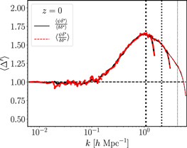
Figure 11. Measured mean mode growth rate with different grid numbers used for FFT. Vertical dotted lines delimit the scales of k = 0.67 kN = 1.08, 2.16, 4.31 h Mpc−1 corresponding to grid number Ngrid = 512, 1024, 2048, respectively. Thinner curves are of finer resolution.
Download figure:
Standard image High-resolution imageAppendix B: Effect of Shot Noise Deduction on S
The shot noises in Pδ
and Pψ
are minuscule, as the number of particles in our simulations is fairly large. As shown in Figure 12, after subtracting the shot noise predicted by the local Poisson approximation (e.g., Pan 2020), the resulting [S(z)/D(z)]/[S(0)/D(0)] does not obey S ∝ D well on scales k < 0.02 h Mpc−1, compared to Figure 6. It is probably due to the fact that on large scales  , a slight change will have a significant influence. But in the quasi-linear regime, the one-loop perturbation theory actually predicts S ∝ D, whether this is a challenge to the way of subtracting shot noises is beyond the scope of this paper and will be left for future research.
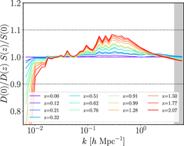
Figure 12. Similar to Figure 6, but [S(z)/D(z)]/ [S(0)/D(0)] of the Pangu simulation is measured with Poisson noises subtracted from Pδ and Pψ .
Download figure:
Standard image High-resolution imageAppendix C: About Cosmic Variance
We have only one realization of the simulation used in this report. To have a concept of the magnitude of cosmic variance in  on small scales, we split the z = 0 snapshot of the Pangu simulation into 8 × 8 × 8 nonoverlapping small subsamples of size Lsub−box = 125 h−1Mpc. The mean mode growth rates of these subsamples are measured and plotted together in Figure 13. One can see that, although the 1σ scatter of
  in the strongly nonlinear regime is not too large, there are indeed quite a few special subsamples whose
  show quite different behaviors (brown solid lines in Figure 13).
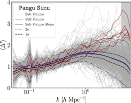
Figure 13. Mean mode growth rates  measured from 512 subsamples, which are generated from the z = 0 snapshot of the Pangu simulation. Individual measurements are plotted as light gray solid lines, while their average and 1σ and 2σ scatters are drawn as black solid, dashed, and dotted lines, respectively. Brown solid lines are of the six selected subsamples that do not have apparent peaks on scales k < 0.67 kN
at all, contrary to the measurement of the entire sample (solid blue line).
measured from 512 subsamples, which are generated from the z = 0 snapshot of the Pangu simulation. Individual measurements are plotted as light gray solid lines, while their average and 1σ and 2σ scatters are drawn as black solid, dashed, and dotted lines, respectively. Brown solid lines are of the six selected subsamples that do not have apparent peaks on scales k < 0.67 kN
at all, contrary to the measurement of the entire sample (solid blue line).
Download figure:
Standard image High-resolution imageFootnotes
- 10
Please see Appendix C to get a rough idea of the influence of cosmic variance on
 .
.
